1

CRITERIA FOR AND STATISTICS OF ELECTRON DIFFUSION REGIONS ASSOCIATED WITH SUB-SOLAR MAGNETIC FIELD RECONNECTION

By F. S. MozerPhysics Department and Space Sciences Laboratory

University of California, Berkeley, Ca., 94720

ABSTRACT

Criteria for identifying electron diffusion regions in magnetic field reconnection events are defined and justified. By employing these criteria and further constraints on the measured parallel electric field, 117 electron diffusion regions have been found in searching through three years of Polar satellite sub-solar data. They exist in filamentary currents in which parallel electric fields and depressed plasma densities are found and where the electron beta is generally less than one. The average parallel electric field in these events is about 30% of the average 38 mV/m perpendicular field. The size of these regions is the order of the electron skin depth or less. These electron diffusion regions are topological boundaries in the plasma and magnetic field line flows because the components of ExB/B2 on their opposite sides are frequently different. These regions are found throughout the magnetopause but mainly on its magnetospheric side and at the magnetospheric separatrix. This may be because the depleted plasma in these regions is not sufficient to carry the filamentary current imposed on it without creating parallel electric fields and the associated microphysics. The divergence of the pressure tensor in the Generalized Ohms Law may be the leading term that balances the parallel electric field because the plasma density is observed to vary significantly in most events. The picture resulting from this data is of a magnetopause that is highly structured and filamentary and very different from a linear, laminar, symmetric, structure sometimes considered in theories or simulations.

INTRODUCTION

By subtraction of Newton’s Second Law for an electron fluid from that for an ion fluid, the Generalized Ohm’s Law is obtained as (Spitzer, 1956)

E+UIxB = cjxB/en −c∇·Pe/en + (mec2/ne2)δj/δt + ηj (1)

where E and B are the electric and magnetic fields, UI is the velocity of an element of ion fluid, j and n are the

current and plasma densities, respectively, η is the resistivity associated with ion-electron interactions, and ∇·Pe is the divergence of the electron pressure tensor. Equivalently, by writing j = ne(UI-Ue) in the first term on the right hand side of equation 1, the UIxB term on the left side is cancelled to give a completely equivalent expression for the Generalized Ohm’s Law as E+UexB = −c∇·Pe/en + (mec2/ne2)δj/δt + ηj (2)

2

where Ue is the velocity of an element of electron fluid. Historically, magnetic field reconnection has been studied by assuming that the last term on the right hand side of these equations dominates the other terms on the right side due to Coulomb or anomalous resistivity (Parker, 1957). More recent simulations (Birn et al, 2001) have considered the importance of the jxB term on the right hand side of equation 1 to develop what is called “Hall MHD physics.” These simulations have been validated by measurements in both space (Deng et al, 2001; Mozer et al, 2002) and the laboratory (Ren et al, private communication, 2005), such that it is now agreed that the physics on the ion skin depth scale, c/ωpI (~100 km at the sub-solar magnetopause), is better understood. One result of this understanding is that the perpendicular current associated with the jxB term is parallel to the reconnection electric field such that there is a significant j·E in the ion skin depth region to convert magnetic field energy over a large scale. However, on this scale, magnetic field lines still move with the ExB/B2 velocity, so the physics in the electron diffusion region on

the electron skin depth scale, c/ωpe (~5 km at the sub-solar magnetopause), must be considered in order to understand magnetic field reconnection. The purposes of this paper are:

− to discuss the necessary conditions for the existence of electron diffusion regions by considering magnetic field line motion from first principles, and

− to present measurements of plasma density, electric fields, and magnetic fields from the Polar satellite that show many electron diffusion regions in a filamentary magnetopause, and

− to discuss statistical properties of these regions.

This data suggests a very different geometry for the electron diffusion region than that which is currently popular. The first results on observations of the electron diffusion region by Polar (Mozer et al, 2003a) and Cluster (Mozer et al, 2005) are presented elsewhere.

MAGNETIC FIELD LINE MOTION FROM FIRST PRINCIPLES

The concept and limitations of magnetic field line motion are reviewed because these results are required to define properties of electron diffusion regions. Rigorously, magnetic field lines neither exist nor move because no experiment can be described to measure these quantities. Instead, both magnetic field lines and their motions are empirical constructs whose usefulness is that they enable one to visualize properties of the solutions to Maxwell’s equations without having to solve these equations. The sole purpose of considering magnetic field line motion is to provide a means for visualizing the time evolution of the magnetic field. Among the infinite number of possible field line motions that produce the correct temporal evolution of the magnetic field (Vasyliunas, 1972), we will select the ExB/B2 velocity and consider under what conditions it

3

produces the same temporal evolution as Maxwell’s equations. To do so, we will consider separately the magnitude and the direction of a magnetic field line after it has moved with the ExB/B2 velocity for the time δt (Longmire, 1963).

1. The magnitude of a magnetic field that evolves with velocity v = ExB/B2

The concept of field line motion implies that a region containing a changing magnetic field experiences this change because field lines move into or out of this region and not because field lines are suddenly created or destroyed. Because field lines are conserved in this picture, they satisfy a continuity equation, which, for B = kBZ is

δBZ/δt + ·(Bv) = 0 (3)

Given the field line velocity v = ExB/B2, the components of Bv are (Bv)X = EY and (Bv)Y=-EX, so

·(Bv) = δEY/δx – δEx/δy (4)

which is the z-component of xE. Because equation 3 is Faraday’s law, the magnitude of the magnetic field evolves as is required by Maxwell’s equations if magnetic field lines move with the ExB/B2 velocity. This statement is exact without approximation and in the presence or absence of plasma, It is noted that any velocity, v', satisfying ·(Bv') = 0 may be added to

ExB/B2 without modifying equation 3. Thus, there are an infinite number of magnetic field line velocities that preserve the magnitude of the magnetic field.

2. The direction of a field line that moves with velocity v = ExB/B2

Fig. 1. Geometry of moving magnetic field lines.

Consider the two surfaces, S1 and S2 in Fig. 1 that are perpendicular to the magnetic field at times t and t + δt. At time, t, a magnetic field line intersects the two surfaces at points a and b. Thus, the vector (b – a) is parallel to B(t). At the

later time, t + δt, point a has moved along S1 at velocity ExB/B2(a) to point a' and it is on the illustrated magnetic field line. Meanwhile, point b has moved along S2 to b' at velocity ExB/B2(b) and it may or may not be on the field line that passes through a'. The question is, what are the constraints on these motions that result in a' and b' being on the same magnetic field

Fig. 1

B(t+δt)

B(t)b′

bt+δt

a′a

S2

S1

4

line, i.e., that result in (b' - a') being

parallel to B(t+δt)?

The vector (b' − a') = (b − a) + (b' − b) − (a' − a).

The terms on the right side of this equation are

(b − a) = εB, because (b − a) is parallel to B.

(a' − a) = [ExB/B2(a)] δt

(b' − b) = [ExB/B2(b)] δt = [ExB/B2

(a) + (b − a)(δExB/B2(a)/δr)] δt = [ExB/B2

(a) + εB· (ExB/B2(a))] δt

where r is a distance along the magnetic field line at time t.

Combining terms gives

(b' − a')/ ε = B + B· (ExB/B2)δt (5)

Also

B' = B(a, t + δt) = B + (δB/δt) )δt +

((ExB/B2)· )Bδt (6)

The problem reduces to finding the constraints on the field line motion that are imposed by the requirement that the right side of equation 5 is parallel to the right side of equation 6 or that their cross-product is zero. To first order in δt, this gives

Bx{δB/δt + (ExB/B2)· )B − B·(ExB/B2)}= 0 (7)

Using the vector identity for xMxN for any two vectors M and N allows rewriting equation (7) as

Bx{δB/δt + x(Bx(ExB/B2)) + B( ·

(ExB/B2)) – (ExB/B2) ·B} = 0 (8)

The last term on the right is zero because

·B = 0 and the next to last term may be omitted because it is parallel to B. Because Bx(ExB/B2) = E−E|| and δB/δt

= − xE, equation 8 becomes

Bx( xE||) = 0 (9)

This is the condition that preserves the direction of the magnetic field during its ExB/B2 motion. While this equation is satisfied by finite parallel electric fields having zero curls, for practical purposes it requires that the parallel electric field be zero when B ≠ 0 in order that field lines moving with ExB/B2 produce the same time evolution of the magnetic field direction as do Maxwell’s equations.

The existence and/or properties of plasma did not enter into the equation 9 requirement that field line motion at ExB/B2 produces the same result as does Maxwell’s equations. Thus, for example, one may consider that magnetic field lines move with ExB/B2 in a vacuum when the parallel electric field is zero. Or, one may consider that field lines move with ExB/B2 in a plasma having no parallel electric field but, in which, the electrons and ions

5

do not move with this velocity because there is a perpendicular pressure gradient.

NECESSARY CONDITIONS FOR OBSERVING THE ELECTRON DIFFUSION REGION

To search experimental data for the presence of electron diffusion regions at the dayside magnetopause, search criteria are defined as:

1. The parallel electric field must be non-zero.

Magnetic field lines that move towards each other with the ExB/B2 velocity will move right through each other if they continued at this velocity. Because this situation neither results in reconnection nor is consistent with Maxwell’s equations, such field lines must not move with the ExB/B2 velocity in the electron diffusion region. Thus, a necessary condition for the existence of the electron diffusion region is that the parallel electric field is non-zero. Because the left side of equation (2) is non-zero in this case, one or more of the terms on the right side of this equation must also be non-zero. Previous measurements suggest that the pressure gradient term may dominate (Mozer et al, 2003a; Mozer et al, 2005).

2. The thickness of the region must be the order of the electron skin depth, c/ωpe.

Vasyliunas (1975) has shown that the electron diffusion region must

have a thickness that is ~c/ωpe, which is the order of 4 kilometers at the sub-solar magnetopause.

3. The perpendicular electric field must be large.

The reconnection electric field associated with a reconnection rate ~0.1vAlfven is ~0.5 mV/m. The perpendicular electric field must be large compared to this value for the electron diffusion region to exert an important influence on reconnection.

4. j·E must be large.The electron diffusion region is a site of conversion of magnetic field energy, so j·E must be large.

5. Accelerated electrons must be produced in the electron diffusion region.

The electromagnetic energy conversion should produce accelerated electron beams.

6. The electron diffusion region must be a topological boundary that separates regions having different ExB/B2 flows.

In static, two-dimensional reconnection, plasma and magnetic field lines ExB/B2 flow in from the left and right and out the top and bottom of the picture. While the ExB/B2 flow in realistic geometries is expected to be more complex, it should still be the case that the electron diffusion region is a boundary separating different flow topologies.

6

An additional requirement for an electron diffusion region might be that it occurs at an x-line where the magnetic field is zero. In the real world, this null magnetic field geometry exists with a vanishingly small probability. Also, there is no prohibition against reconnection occurring in finite magnetic fields, so there are no limitations on the field strength or the electron beta that are imposed on a search for electron diffusion regions.

For purposes of this paper, “electron diffusion region” is any region satisfying the above conditions. This definition includes locales away from the magnetopause that contain parallel electric fields, such as the auroral acceleration region. The microphysics in such regions is the same as that associated with reconnection and it is equally correct in the auroral acceleration region that two particles on the same field line before passing through such a region are likely to be on different field lines after passing through the region, due to “magnetic field line slippage.” Thus, the difference between different regions containing parallel electric fields is largely one of terminology and not of micro-physics. The data from the Polar satellite allow determination of the parallel electric field because it contains a three-component E-field measurement. This contrasts with the two-component data from the Cluster satellite that do not permit determination of the parallel electric field. However, the EDI experiment on Cluster (Paschmann et al, 1997) produces measurements of natural electrons at two pitch angles with an eight millisecond time resolution,

thereby providing data that satisfies criterion 5, above (Mozer et al, 2005). Thus, the combination of data from the two spacecraft satisfies all of the above criteria.

M E A S U R E M E N T S O F T H E PARALLEL ELECTRIC FIELD ON POLAR

From February through mid-May in 2001, 2002, and 2003, the 9.5 RE geocentric apogee of the Polar satellite was at low latitudes on the dayside of the magnetosphere. Electric fields at magnetopause crossings were examined during these times for candidate electron diffusion region events. Because a non-zero parallel electric field is required, the parallel electric field measurement was closely scrutinized. It may be uncertain because:

− it is as small as 10% of the perpendicular electric field, so geometric misalignments can produce apparent parallel electric fields,

− the magnetic field is not measured with the time resolution of the electric field, so the B-field is linearly interpolated to the times of E-field measurements. If the rapidly changing magnetic field does not vary linearly, apparent parallel electric fields can result,

− the short, spin-axis electric field measurement (Harvey et al, 1995) is uncertain due to its proximity to perturbations from the spacecraft. This may introduce noise in the parallel field estimate that can be comparable to the observed parallel field, depending on the

7

geometry of the situation. This is the source of the largest uncertainty in the parallel electric field measurement.

Because the spacecraft was in a cartwheel mode, one of the pair of on-axis sensors was shadowed by the spacecraft in the vicinity of the dawn-dusk orbit, and the resulting data is not usable. However, in the noon-midnight orbit, there is a high level of symmetry between these sensors, the spacecraft, its photoemission, and the sun. This causes any perturbation from photoemission, for example, to be the “same” on the two on-axis sensors, so this perturbation cancels when the potential difference is measured. However, one of the on-axis sensors is closer than the other to the center of the 1/r potential from the charged spacecraft because the despun platform extends on one side of the spacecraft to spoil the axial symmetry. For this reason, it is necessary to subtract ~200 millivolts from the measured potential difference along the spin axis to obtain a field that is small in regions where the spin-plane-measured fields are small. Other than adjusting this offset, there are no special corrections made to the on-axis measurements.

Fig. 2 illustrates the technique for validating the parallel electric field measurement. The data are presented in a field-aligned coordinate system in which the Z-axis is parallel to the magnetic field direction while the X-axis is perpendicular to B in the plane containing the magnetic field line and it is positive inwards. The Y-axis defines the third component of this right hand coordinate system by being perpendicular to B and pointing generally

in the westward direction. The field components in this coordinate system are obtained in three ways:

− by using the measured three components of the electric field

− by discarding the on-axis measurement and assuming that the parallel electric field is zero

− by discarding the on-axis measurement and assuming that the component of the electric field in this direction is zero.

Fig. 2. Electric field components in a magnetic-field-aligned coordinate system to illustrate the method of validating the parallel electric field measurement.

Panels a), b), and c) give the X-component of the electric field computed in the three ways, panels d), e), and f) give the Y-component, and panels g) and h) give the Z-component (the Z-component computed under the assumption that E·B = 0 is not given because it is zero). The figure contains four seconds of data at a

0 42

TIME (SECONDS) AFTER 12:53:56 ON FEBRUARY 17, 2003

Fig. 2

a)

b)

c)

d)

e)

f )

g)

h)

8

geocentric altitude of 9.47 earth radii, magnetic local time of 1320, and magnetic latitude of -14.2 degrees. Note that the scales of the electric field plots differ for the different field components. The values of EX computed by the three methods are essentially identical because the X-direction in magnetic field aligned coordinates happened to be perpendicular to the spacecraft spin axis. The value of EY computed by assuming that the on-axis field was zero (panel f)) is small because the Y-direction was nearly parallel to the spin axis. The parallel electric fields in panels g) and h) are non-zero and similar because the parallel electric field comes mainly from measurements made by the long spin plane sensors. EY obtained from direct measurements (panel d)) and from assuming that the parallel electric field was zero (panel e)) differ by factors as large as four. This is strong evidence that the measured parallel electric field is real because the Y-component requires a major adjustment if it is to be compatible with the assumption that the parallel electric field was zero.

Examples satisfying the above criteria for yielding an acceptable parallel field were found in more than 100 of the ~1000 cases that were examined.

FURTHER EXAMPLES OF ELECTRON DIFFUSION REGIONS

Fig. 3 gives the plasma density, the magnetic field and the components of ExB/B2 for the same four second interval as in Fig. 2. The plasma density in panel a) decreased from about 1.5 to 0.1 cm-3 during the fraction of a second that the electron diffusion region was crossed.

The magnetic field components of panels b), c), and d), (plotted with different zero level suppressions) show that the spacecraft was at or near the magnetospheric separatrix, because the Z-component had the magnetospheric sign and magnitude. The components of ExB/B2, illustrated in panels f), g), and h), changed across the diffusion region by as much as 150 km/sec, indicating that the fields and flows on one side of the boundary were independent of those on the other side. (The components of ExB/B2 have been deleted in the region of the parallel electric field because they are not meaningful in terms of either electron or field line flow.) The electron beta for this event was about 0.005. The average parallel electric field of Fig. 2 was about 30% of the perpendicular field but there were times when the parallel field exceeded the perpendicular field. The temporal variations of the field components were at the 25 millisecond resolution of the measurement, which, for an assumed boundary velocity of 50 km/sec, yields a thickness of the spiky fields less than the 5-15 km electron skin depth. The total magnetic field of panel e) in Fig. 3 did not change across the electron diffusion region. Thus, the steps in BY and BZ in panels c) and d) must have been due to field aligned currents. For a magnetic field change of 9 nT in 0.7 seconds and an assumed boundary speed of 50 km/sec, Ampere’s law gives a parallel current density of 0.1 μamps/m2. Combining this current density with an average parallel electric field of 8 mV/m and plasma density of 0.2 cm-3 gives jllEll/n ≈ 50 keV/particle-second. Thus, a typical electron that receives this energy

9

while residing in the electron diffusion region for ~5 milliseconds will gain a few hundred eV of energy.

Fig. 3. Plasma density, magnetic field, and components of ExB/B2 during the time interval illustrated in Fig. 2.

An extremely rare example of a magnetosheath separatrix is given in Figs. 4 and 5 at a time when the spacecraft was at an altitude of 9.38 RE, magnetic local time of 1145, and magnetic latitude of 6.25 degrees. Prior to the event of interest in Fig. 5, the Z-component of the magnetic field in Fig. 4 (panel d)) changed from +80 nT to -80 nT in steps, signifying the crossing of a magnetopause containing a filamentary current. It is noted that the magnetic field in GSE

coordinates in this figure is nearly in the minimum variance coordinates because BX of panel b) is small and nearly non-changing while the maximum variance occurs in BZ. Also, this was a rotational discontinuity with a mostly parallel current because the total field of panel e) did not change very much. The data of

Fig. 4. Magnetic field and plasma density during a magnetopause crossing crossing from the magnetosphere to the magnetosheath.

Fig. 5 were collected at the time of the dashed line in Fig. 4, during which the magnetic field was near its magnetosheath value. Panel a) of Fig. 5 shows that the magnetosheath plasma density was unusually low and that it changed significantly as the electron diffusion region was crossed. Panels b), c), and d) of this figure give the electric field components in the field-aligned coordinate system. No change of ExB/B2

0 2 4

TIME (SECONDS) AFTER 12:53:56 ON FEBRUARY 17, 2003

Fig. 3

a)

b)

c)

d)

e)

f )

g)

h)

0 10 20 30 40

TIME (SECONDS) AFTER 05:52:10 ON APRIL 1, 2001

Fig. 4

a)

b)

c)

d)

e)

10

greater than about 50 km/sec was observed at this crossing. The spiky electric field structures had thicknesses less than or the order of the electron skin depth. The electron plasma beta was about 0.01 during this event. For an assumed boundary speed of 25 km/sec, jllEll/n was about 50 keV/particle-second with an uncertainty of at least a factor of two because the boundary speed is not known and the magnetic field and plasma density were not measured with sufficient time resolution.

Fig. 5. Field measurements made as a magnetosheath electron diffusion region passed over the Polar spacecraft.

An example of an electron diffusion region near the center of the magnetopause is described in Figs. 6 and 7. The spacecraft was at an altitude of 8.92 RE, magnetic local time of 1325, and

magnetic latitude of 37.67 degrees. Fig. 6 gives the plasma density (panel a)), the three components of the magnetic field (panels b), c), and d)), and the total magnetic field intensity (panel e)). During the 22 second interval of this figure, the density increased from a magnetospheric value of ~1 cm-3 to the magnetosheath value of ~18 cm-3 while the Z-component of the magnetic field decreased from its ~55 nT magnetospheric value to the -30 nT magnetosheath value. Near the center of the crossing, at the 8 nT minimum of the total magnetic field, the plasma density decreased and then

Fig. 6. Magnetic field components and plasma density measured at an electron diffusion region near the center of the magnetopause.

increased by factors of about 4 in less than one second. This region is expanded in the six second plot of Fig. 7, which also includes the components of the electric

0 5 10 15

TIME (SECONDS) AFTER 00:18:20 ON FEBRUARY 27, 2001

a)

b)

c)

d)

e)

Fig. 6

0 0.5 1.0 1.5

TIME (SECONDS) AFTER 05:52:42.5 ON APRIL 1, 2001

a)

b)

c)

d)

Fig. 5

11

field in field-aligned coordinates and ExB/B2 in GSE coordinates. (The components of ExB/B2 have been deleted in the region of the parallel electric field because they are not meaningful.)

Fig. 7. Electric field and ExB/B2 flow measurements made at an electron diffusion region located near the center of the magnetopause.

Although the magnitude of the perpendicular electric field was small compared to typical values (panels b) and c)), the parallel field was the typical 5-8 mV/m (panel d)) and it was larger than the perpendicular field at the two large plasma density changes near 13 and 17 seconds in the plots. The ExB/B2 components of panels e), f), and g), show that the plasma and magnetic field perpendicular flows changed by ~100 km/sec across the electron diffusion region, signifying that

the fields on the two sides of the boundary were uncoupled. The electron beta during this event was greater than 2.

STATISTICS OF SUB-SOLAR ELECTRON DIFFUSION REGIONS

During the three year search for sub-solar electron diffusion regions, 117 events satisfying rigorous criteria on the parallel electric field were identified. These events do not occur randomly in time; rather they come in bunches. For example, 70 of the 117 events were found in 12 of the ~400 orbits that were examined. Most of the events occurred in current filaments and were associated with significant changes of the plasma density. Most of the magnetopause crossings did not yield verifiable electron diffusion regions.

Fig. 8. Locations in magnetic local time and magnetic latitude of electron diffusion region events.

-40

-20

0

20

40

8 10 12 14 16

MAGNETIC LOCAL TIME

MA

GN

ETIC

LA

TITU

DE

Fig. 8

0 5 10 15 20 25

TIME (SECONDS) AFTER 00:18:25 ON FEBRUARY 27, 2001

a)

b)

c)

d)

e)

f )

g)

Fig. 7

mV/

mm

V/m

mV/

m

12

Fig. 9. Clock angle versus magnetic l a t i t u d e o f t h e r e c o n n e c t i n g magnetopauses in which electron diffusion regions were found.

Fig. 8 gives the electron diffusion region locations in magnetic latitude and magnetic local time. The sub-solar point is in the center of this plot and events were found at all local times and latitudes at which the spacecraft encountered the magnetopause. This includes the region from 0800 to 1600 in magnetic local time and -40 to +40 degrees of magnetic latitude.

Fig. 9 shows the clock angle (the angle between the asymptotic magnetosheath and magnetospheric magnetic field vectors) as a function of magnetic latitude for the magnetopause reconnection events that contained electron diffusion regions. A wide range of clock angles was observed at all latitudes reached by the spacecraft trajectory. The apparent number of large clock angles may be a selection effect because the signature of such crossings is much clearer than for

those having a small clock angle. Some of the small clock angles may be inaccurate because the turbulence in the magnetic field made clock angle measurements uncertain.

Fig. 10. Perpendicular electric field magnitudes measured in electron diffusion regions.

A histogram of the perpendicular electric field magnitudes in electron diffusion regions is given in Fig. 10. While the observed fields ranged up to 100 mV/m, the average perpendicular electric field was 38 mV/m, which is one or two orders-of-magnitude larger than the reconnection electric field found in theories and simulations.

The ratio of the parallel to perpendicular electric fields is plotted in Fig. 11. The smallest parallel electric fields were 10% of the perpendicular field because the criteria on an event included the requirement that the parallel field be at least this big in order that geometric errors could not produce an apparent parallel

0

5

10

15

20

25

30

35

0 20 40 60 80 100

PERPENDICULAR ELECTRIC FIELD, mV/m

NU

MBE

R O

F EV

ENTS

Fig. 10

-40

0

40

0 45 90 135 180

CLOCK ANGLE

MA

GN

ETIC

LA

TITU

DE

Fig. 9

13

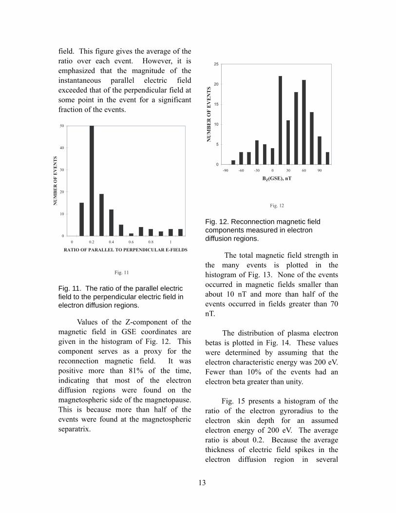
field. This figure gives the average of the ratio over each event. However, it is emphasized that the magnitude of the instantaneous parallel electric field exceeded that of the perpendicular field at some point in the event for a significant fraction of the events.

Fig. 11. The ratio of the parallel electric field to the perpendicular electric field in electron diffusion regions.

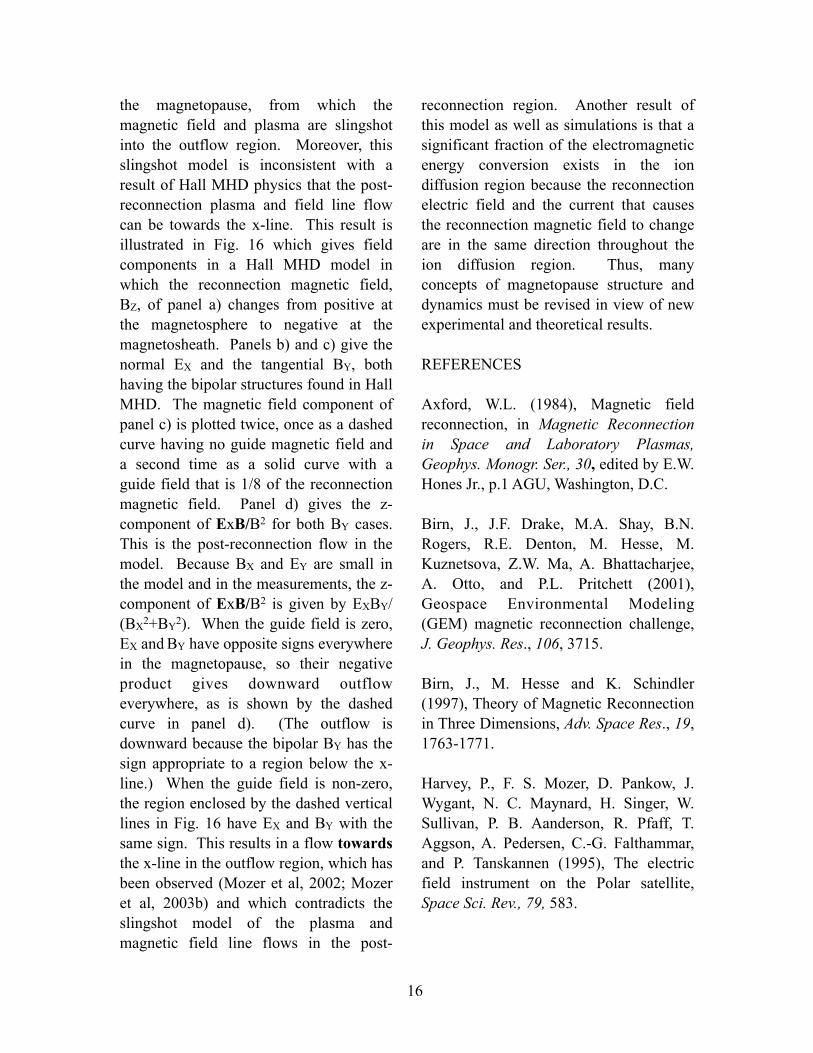
Values of the Z-component of the magnetic field in GSE coordinates are given in the histogram of Fig. 12. This component serves as a proxy for the reconnection magnetic field. It was positive more than 81% of the time, indicating that most of the electron diffusion regions were found on the magnetospheric side of the magnetopause. This is because more than half of the events were found at the magnetospheric separatrix.

Fig. 12. Reconnection magnetic field components measured in electron diffusion regions.

The total magnetic field strength in the many events is plotted in the histogram of Fig. 13. None of the events occurred in magnetic fields smaller than about 10 nT and more than half of the events occurred in fields greater than 70 nT.

The distribution of plasma electron betas is plotted in Fig. 14. These values were determined by assuming that the electron characteristic energy was 200 eV. Fewer than 10% of the events had an electron beta greater than unity.

Fig. 15 presents a histogram of the ratio of the electron gyroradius to the electron skin depth for an assumed electron energy of 200 eV. The average ratio is about 0.2. Because the average thickness of electric field spikes in the electron diffusion region in several

0

5

10

15

20

25

-90 -60 -30 0 30 60 90

BZ(GSE), nT

NU

MBE

R O

F EV

ENTS

Fig. 12

0

10

20

30

40

50

0 0.2 0.4 0.6 0.8 1

RATIO OF PARALLEL TO PERPENDICULAR E-FIELDS

NU

MBE

R O

F EV

ENTS

Fig. 11

14

examples is 30% of the electron skin depth (Mozer, 2005), the gyroradius can be comparable to the thickness of large electric field regions and this might exert a significant impact on the microphysics.

Fig. 13. The total magnetic field measured in electron diffusion regions.

Fig. 14. The plasma electron beta measured in electron diffusion regions.

Fig. 15. The ratio of the electron gyroradius to the electron skin depth for an assumed electron energy of 200 eV.

DISCUSSION

By definition, the necessary conditions for the observation of an electron diffusion region are that the parallel electric field is non-zero, j·E is large, the thickness of the region is ~ c/ωpe, the perpendicular electric field is large compared to the typical reconnection electric field, and the region is a boundary separating different plasma and magnetic field line flows on its two sides. Polar satellite events are shown to satisfy all these criteria. An additional criterion is that accelerated electrons should be observed in the electron diffusion region. The Polar particle instruments do not have the time resolution to test this requirement. However, Cluster data have

0

10

20

30

0 0.1 0.2 0.3 0.4 0.5 0.6

ELECTRON GYRORADIUS/SKIN DEPTH

NU

MBE

R O

F EV

ENTS

Fig. 15

0

10

20

30

40

50

0.001 0.01 0.1 1 10

ELECTRON BETA

NU

MBE

R O

F EV

ENTS

Fig. 14

0

5

10

15

20

25

0 20 40 60 80 100

TOTAL MAGNETIC FIELD, nT

NU

MBE

R O

F EV

ENTS

Fig. 13

15

shown the existence of accelerated electrons and have produced an estimate of the average thickness of the electron diffusion region as ~0.3c/ωpe in the direction of its motion and more than 1000 kilometers in the plane perpendicular to its motion (Mozer et al, 2005). Thus, the combination of the Polar and Cluster data satisfy the requirements to identify the objects studied in this paper as electron diffusion regions.

A possible explanation for the more frequent occurrence of electron diffusion regions at the magnetospheric side of the magnetopause is that the current imposed on the local region by its filamentary nature is too large to be carried by the low density plasma near the magnetosphere so parallel electric fields and the associated microphysics are required to maintain current continuity.

It is again noted that the electron beta was less than one for more than 90% of the electron diffusion regions and that most events occurred in filamentary currents in which the plasma density was depleted. These features will be significant in any theory of these regions.

The electron diffusion regions described in this paper are not shown to be responsible for the connection of terrestrial magnetic field lines with interplanetary magnetic field lines. This is in part due to the impossibility of showing such a connection with low resolution data from a single satellite and in part due to the possibility that some of the events may not have achieved this result. Even in this case, such events are interesting because they include the same

micro-physics as is found in regions that do result in the connection of terrestrial and interplanetary magnetic field lines. The picture resulting from this data is of a magnetopause that is highly structured and filamentary and that contains many electron diffusion regions, which is similar to that described in s eve ra l s imu la t ions (Ma and Bhattacharjee, 1996; Onofri et al, 2004; Karimabadi et al, 2005, Drake, private communication, 2005) and very different from a linear, laminar, symmetric, structure sometimes considered in theories or simulations.

Fig. 16. Electric and magnetic fields in an idealized Hall MHD model of the magnetopause, showing that post-reconnection flow towards the x-line occurs when the guide magnetic field is non-zero.

These results contradict the model of a single reconnection region at the center of

0 0.2 0.4 0.6 0.8 1

DISTANCE ACROSS THE MAGNETOPAUSEMAGNETOSPHERE MAGNETOSHEATH

Fig. 16

a)

b)

c)

d)

16

the magnetopause, from which the magnetic field and plasma are slingshot into the outflow region. Moreover, this slingshot model is inconsistent with a result of Hall MHD physics that the post-reconnection plasma and field line flow can be towards the x-line. This result is illustrated in Fig. 16 which gives field components in a Hall MHD model in which the reconnection magnetic field, BZ, of panel a) changes from positive at the magnetosphere to negative at the magnetosheath. Panels b) and c) give the normal EX and the tangential BY, both having the bipolar structures found in Hall MHD. The magnetic field component of panel c) is plotted twice, once as a dashed curve having no guide magnetic field and a second time as a solid curve with a guide field that is 1/8 of the reconnection magnetic field. Panel d) gives the z-component of ExB/B2 for both BY cases. This is the post-reconnection flow in the model. Because BX and EY are small in the model and in the measurements, the z-component of ExB/B2 is given by EXBY/(BX2+BY2). When the guide field is zero, EX and BY have opposite signs everywhere in the magnetopause, so their negative product gives downward outflow everywhere, as is shown by the dashed curve in panel d). (The outflow is downward because the bipolar BY has the sign appropriate to a region below the x-line.) When the guide field is non-zero, the region enclosed by the dashed vertical lines in Fig. 16 have EX and BY with the same sign. This results in a flow towards the x-line in the outflow region, which has been observed (Mozer et al, 2002; Mozer et al, 2003b) and which contradicts the slingshot model of the plasma and magnetic field line flows in the post-

reconnection region. Another result of this model as well as simulations is that a significant fraction of the electromagnetic energy conversion exists in the ion diffusion region because the reconnection electric field and the current that causes the reconnection magnetic field to change are in the same direction throughout the ion diffusion region. Thus, many concepts of magnetopause structure and dynamics must be revised in view of new experimental and theoretical results.

REFERENCES

Axford, W.L. (1984), Magnetic field reconnection, in Magnetic Reconnection in Space and Laboratory Plasmas, Geophys. Monogr. Ser., 30, edited by E.W. Hones Jr., p.1 AGU, Washington, D.C.

Birn, J., J.F. Drake, M.A. Shay, B.N. Rogers, R.E. Denton, M. Hesse, M. Kuznetsova, Z.W. Ma, A. Bhattacharjee, A. Otto, and P.L. Pritchett (2001), Geospace Environmental Modeling (GEM) magnetic reconnection challenge, J. Geophys. Res., 106, 3715.

Birn, J., M. Hesse and K. Schindler (1997), Theory of Magnetic Reconnection in Three Dimensions, Adv. Space Res., 19, 1763-1771.

Harvey, P., F. S. Mozer, D. Pankow, J. Wygant, N. C. Maynard, H. Singer, W. Sullivan, P. B. Aanderson, R. Pfaff, T. Aggson, A. Pedersen, C.-G. Falthammar, and P. Tanskannen (1995), The electric field instrument on the Polar satellite, Space Sci. Rev., 79, 583.

17

Karimabadi, H., W. Daughton, and K.B. Quest (2005), Anti-parallel versus component merging at the magnetopause: Current bifurcation and intermittent reconnection, J. Geophys. Res., 110, A03213, doi:10, 1029/2004JA010750.

Longmire, C.L. (1963), Elementary plasma physics, Interscience Publishers, John Wiley and Sons, New York.

Ma, Z.W. and A. Bhattacharjee (1996), Fast impulsive reconnection and current sheet intensification due to electron pressure gradients in semi-collisional plasmas, Geophys. Res. Lett., 23, 1673.

Mozer, F. S., S. D. Bale, and T. D. Phan (2002), Evidence of diffusion regions at a sub-solar magnetopause crossing, Phys. Rev. Lett., 89, 015002, doi: 10.1103/PhysRevLett.89.015002.

Mozer, F. S., S. D. Bale, T. D. Phan, and J. A. Osborne (2003a), Observations of electron diffusion regions at the subsolar magnetopause, Phys. Rev. Lett., 91, 245002.

Mozer, F.S. T. D. Phan, and S. D. Bale (2003b), The complex structure of the reconnecting magnetopause, Phys. Plasmas, 10, 2480.

Mozer, F. S., S. D. Bale, J. P. McFadden, and R. B. Torbert (2005), Observations of magnetic field reconnection sites at the sub-solar magnetopause, Phys. Rev. Lett., in press.

Onofri, M., L. Primavera, F. Malara, and P. Veltri (2004), Three-dimensional

simulations of magnetic reconnection in slab geometry, Phys. Plasmas, 11.

Parker, E.N. (1957), Sweet’s mechanism for merging magnetic fields in conducting fluids, J. Geophys. Res., 62, 509.

Parker, E.N. (1963), The solar flare phenomenon and the theory of reconnection and annihilation of magnetic fields, Ap. J. Suppl., 8, 177.

Paschmann, G., G. Melzner, R. Frenzel, H. Vaith, P. Parigger, U. Pagel, O. H. Bauer, G. Haerendel, W. Baumjohann, N. Scopke, R. B. Torbert, B. Briggs, J. Chan, K. Lynch, K. Morey, J. M. Quinn, D. Simpson, C. Young, C. E. McIlwain, W. Fillius, S. S. Kerr, R. Mahieu, and E. C. Whipple (1997), The electron drift instrument for Cluster, Space Sci. Rev., 79, 233.

Schindler, K, M. Hesse and J. Birn (1988), General Magnetic Reconnection, Parallel Electric Fields, and Helicity, J. Geophys. Res., 93, 5547-5557.

Sonnerup, B.U.O., et al. (1984), Reconnection of magnetic fields, in Solar Terrestrial Physics: Present and Future, NASA Ref. Pub. 1120, edited by D.M. Butler and K. Papadapolous.

Spitzer, L. Jr. (1956), Physics of fully ionized gases, Interscience tracts on physics and astronomy, Editor R.E. Marshak, Interscience Publishers, Inc., New York.

Vasyliunas, V.M. (1972), Nonuniqueness of magnetic field line motion, J. Geophys. Res., 77, 6271.

18

Vasyliunas, V.M. (1975), Theoretical models of magnetic field line merging, Rev. Geophys. Space Phys., 13, 303.