Crittical issuees in e

Outcom9-10

Luisa M

estim

mes of anNovemb

Marelli, D

EUR 2

matingemis

n expert cer 2010,

eclan MuRobe

24816 EN - 20

g ILUssionconsultatIspra (Ita

ulligan art Edwar

11

Cns

ionaly)

and rds

2  

The mission of the JRC-IE is to provide support to Community policies related to both nuclear and non-nuclear energy in order to ensure sustainable, secure and efficient energy production, distribution and use.

European Commission Joint Research Centre Institute for Energy Contact information Joint Research Centre Institute for Energy Renewable Energy Unit TP 450 I-21027 Ispra (VA) Italy E-mail: luisa.marelli@jrc.ec.europa.eu Tel.: +39 0332 78633 Fax: +39 0332 785869 http://re.jrc.ec.europa.eu/bf-tp/ http://www.jrc.ec.europa.eu/ Legal Notice Neither the European Commission nor any person acting on behalf of the Commission is

responsible for the use which might be made of this publication.

Europe Direct is a service to help you find answers to your questions about the European Union

Freephone number (*): 

00 800 6 7 8 9 10 11

(*) Certain mobile telephone operators do not allow access to 00 800 numbers or these calls may be billed. 

A great deal of additional information on the European Union is available on the Internet. It can be accessed through the Europa server http://europa.eu/ JRC 64429 EUR 24816 EN ISBN 978-92-79-20240-7 (print) ISBN 978-92-79-20241-4 (pdf)ISSN 1018-5593 (print) ISSN 1831-9424 (online)doi:10.2788/19870 Luxembourg: Publications Office of the European Union © European Union, July 2011 Reproduction is authorised provided the source is acknowledged Printed in Italy

3  

The views expressed in this report are those of the experts who participated to the 

workshop only, and do not represent the opinion of the Commission 

Critical issues in estimating ILUCemissions

Outcomes of an expert consultation9-10 November 2010, Ispra (Italy)

4  

Acknowledgments:

This report is the result of the consultations with worldwide experts and the inputs from all of them are acknowledged. We thank in particular:

Aaron Levy (US-EPA) Aljosja Hooijer (Deltares, The Netherlands) Andre Nassar (ICONE, São Paulo, Brasil) Bart Dehue (Ecofys International BV, Utrecht, The Netherlands Bruce Babcock (Center for Agricultural and Rural Development, Iowa State University, U.S.) Caspar Verwer (Alterra, Wageningen UR, The Netherlands) Chris Malins (the ICCT, Washington D.C, U.S.) David Laborde (IFPRI, Washington D.C, U.S.) Elke Stefhest (PBL, The Hague, The Netherlands) Jacinto Fabiosa (FAPRI-CARD, Iowa State University, U.S.) Jannick Schmidt (2.-0 LCA Consultants, Aalborg East, Denmark) Johannes Schmid (University of Natural resources and Life Sciences, Wien, Austria) John Sheehan (Initiative for Renewable Energy & the Environment, University of Minnesota, U.S.) Juergen Reinhard (EMPA, Duebendorf, Switzerland) Klaus Nottinger (APAG, The European Oleochemicals & Allied Products Group, Bruxelles, Belgium) Koen Overmars (PBL, The Hague, The Netherlands) Lulie Melling (Tropical Peat Research Laboratory, Malaysia) Marijn van der Veld (IIASA, Laxenburg, Austria) Martin Herold (Laboratory of Geo-Information Science and Remote Sensing, Wageningen University) Michael O’Hare (Goldman School of Public Policy, University of California – Berkeley, U.S.) Richard Tipper (Ecometrica, U.K.) Roman Keeney (Department of Agricultural Economics, Purdue University, US.) Steffen Fritz (IIASA Laxenburg, Austria) Susan Page (Department of Geography, University of Leicester, UK) Timothy Searchinger (Woodrow Wilson School, Princeton University, U.S.) Warwick Lywood (Ensus, U.K.) Wolfram Schlenker (Department of Economics, Columbia University, U.S.) Fabien Ramos (EC JRC-IES) Fabio Monforti Ferrario (EC JRC- IE) Frederich Achard (EC JRC-IES) Hans Jurgen Stibig (EC JRC-IES) Miguel Brandao (EC JRC-IES) Renate Koeble (EC JRC-IES) Roland Hiederer (EC JRC – IES) Oyvind Vessia (EC DG ENER) Ignacio Vazquez (EC DG CLIMA) Ian Hodgson (EC DG CLIMA) Bertin Martens (EC DG TRADE)  A special thank you goes to our colleague Alison Burrel for her suggestions and reviews of this document.  

5  

ContentsSummary ........................................................................................................................................................... 9 1. Background ................................................................................................................................................. 13 2. Assessment of Land Use Changes ............................................................................................................... 14 2.1Cropland allocation ............................................................................................................................... 14 2.1.1 Available methodologies ............................................................................................................... 14 2.1.2 Discussion of the methodologies .................................................................................................. 17 2.1.3 Drivers for extra land allocation .................................................................................................... 19 2.1.4 Exclusion of protected areas from available areas ........................................................................ 19 2.1.5 Land conversion ............................................................................................................................. 20 

3. GHG emissions from Land Use Changes ..................................................................................................... 23 3.1 Methodologies to calculate GHG emissions ......................................................................................... 23 3.2 Accounting for foregone C sequestration ............................................................................................ 24 3.3 GHG emissions from draining peatlands .............................................................................................. 25 3.5 Adequate representation of land availability (e.g. CIS and EU) ........................................................... 28 3.6 Uncertainties in datasets ...................................................................................................................... 30 

4 Agro‐economic modelling and uncertainties: ............................................................................................. 31 4.1 Intensification ....................................................................................................................................... 32 4.1.1Impact of pasture converted to cropland ...................................................................................... 32 4.1.2 Contribution of double cropping to increased production ........................................................... 34 

4.2 Yields ..................................................................................................................................................... 34 4.2.1 Importance of yields in models ..................................................................................................... 34 4.2.2 Meeting biofuel demand through yield increases......................................................................... 35 4.2.3 GHG emissions from increased fertilizer application .................................................................... 37 4.2.4 Comparison of yields on new cropland to yields on existing cropland ......................................... 37 4.2.5 Crop displacement ......................................................................................................................... 39 4.2.6 Effect of price on yields and rate of yield increase ....................................................................... 40 4.2.7 Yield increase vs. Area increase ..................................................................................................... 41 4.2.8 Uncertainty in yield elasticities and risk for policy ........................................................................ 42 

4.3ILUC reductions ..................................................................................................................................... 42 4.3.1 ILUC reduction from by‐products .................................................................................................. 42 4.3.2 ILUC reduction from less food consumption. ................................................................................ 44 

4.4 Food commodity markets ..................................................................................................................... 46 5.  Sensitivity and uncertainties in modelling studies ................................................................................ 50 5.1 ILUC and cost of carbon abatement ..................................................................................................... 53 5.2 Mitigating the risk of unwanted indirect effects .................................................................................. 54 

6.  Policy recommendations on ILUC ......................................................................................................... 56   

6  

Table of Figures  Figure 1: Schematic representation of JRC methodology to allocate extra cropland demand (slide 

presented during the expert consultation) ........................................................................................................... 15 Figure 2 Land use change transition matrix (presented by J. Schmidt – 2.‐0 LCA Consultants) .................... 17 Figure 3 llustration of principle and mass balance of land tenure process .................................................... 17 Figure 4 High percentage of change for most land cover classes [from H. Gibbs]......................................... 18 Figure 5 Sampled areas in the tropics (from Gibbs et al., 2010) .................................................................... 20 Figure 6: carbon emissions from peatland drainage [presented by A. Hooijer, Deltares] ............................. 21 Figure 7: global distribution of peatland areas and C store [presented by S. Page – Univ. of Leicester] ...... 22 Figure 8: comparison of 1980 and 2007 land use maps for Sarawak region (Malaysia) [Source: Forestry 

Department of Sarawakpresented by H.J.Stibig – JRC) ......................................................................................... 22 Figure 9: Afforestation rates in the EU assumed by different models [presented by W. Lywood – Ensus]. . 24 Figure 10: peat subsidence level [presented by A. Hoojier, Deltares] ........................................................... 26 Figure 11: Emissions from peat oxidation as a function of water depth [presented by A. Hoojier, Deltares]

 ............................................................................................................................................................................... 27 Figure 12: Fire map (2010) and forest map (2007) in Sumatra [presented by S. Page, Univ. of Leicester] ... 27 Figure 13: Reduction of C sequestration and C release due to peat oxidation and combustion associated 

with all forms of land use change on Southeast Asian peatlands [presented by S. Page – Univ. of Leicester].... 28 Figure 14: Example of IIASA geo‐Wiki tool for Comparison of global land cover products [presented by S. 

Fritz – IIASA] .......................................................................................................................................................... 29 Figure 15: Number of double cropped soybean acres in the US (million acres) [presented by J. Fabiosa –

FAPRI CARD] .......................................................................................................................................................... 34 Figure 16: Crop yields growth needed to provide food and biofuels without deforestation [presented by T. 

Searchinger – Princeton University] ..................................................................................................................... 35 Figure 17: Corn area and (N) fertilizer use [presented by J. Fabiosa – FAPRI CARD] ..................................... 36 Figure 18: Yields in US specific counties with or without cropland expansion [presented by B. Babcock – 

FAPRI) .................................................................................................................................................................... 38 Figure 19: Change in planted acres from 2006 to 2009 in the U.S. [presented by B. Babcock – FAPRI) ....... 40 Figure 20 Rate‐of‐area increase against rate‐of‐yield increase (Presented by W.Lywood – source FAOSTAT).

 ............................................................................................................................................................................... 41 Figure 21: Fraction of gross feedstock saved by by‐products (tonnes) Presented by JRC‐IE) ........................ 44 Figure 22: Demand‐change and production‐change (supply) of vegetable oil – Presented by JRC‐IE. ......... 48 Figure 23 Demand and supply of cereals – EU and North Africa (Presented by W. Lywood ‐ Ensus)............ 48 Figure 24 Decomposition between yield and land extension [presented by D. Laborde – IFPRI] ................. 50 Figure 25: results of Monte Carlo analysis on Land Use emissions from IFPRI – MIRAGE model [Presented 

by D. Laborde – IFPRI] ........................................................................................................................................... 51 Figure 26 : Uncertainty analysis on ILUC Emissions from US corn ethanol [presented by M. O’Hare] ......... 52 Figure 27 Abatement costs as a function of ILUC emissions (presented by C. Malins – The ICCT) ................ 53 Figure 28 GHG emissions from several feedstocks compared to fossil fuel comparator. [presented by B. 

Dehue – Ecofys] ..................................................................................................................................................... 54 Figure 29:  Fossil fuels substitution according to different scenarios (presented by J. Reinhard – EMPA) ... 55 Figure 30 : GHG saving potential in Switzerland (presented by J. Reinhard – EMPA) ................................... 55 

  

7  

LIST of ACRONYMS  AEZ    Agro‐Ecological Zones ARB   Air Resources Board BLUM  Brazilian Land Use Model CAP   Common Agricultural Policy  CARD   Center for Agricultural and Rural Development CGE   Computable general equilibrium CET   Constant Elasticity of Transformation CIS    Commonwealth of Independent States CLUE   Conversion of Land Use and its Effects Modelling Framework COSIMO   Commodity Simulation Model CRP   Conservation Reserve Programme  DDGS  Dried Distillers Grains with Solubles  DG AGRI  General of Agriculture  DG CLIMA  Directorate‐General for Climate Action DG ENER  Directorate‐General for Energy  DG TRADE  Directorate‐General for Trade EC    European Commission EMPA  Eidgenössische Materialprüfungs‐ und Forschungsanstalt EPA   US Environmental Protection Agency EU    European Union FAO  Food and Agriculture Organization of the United Nations  FAPRI  Food and Agricultural Policy Research Institute FASOM  Forest and Agricultural Sector Optimization Model  FAO   Food and Agriculture Organization of the United Nations FQD  Fuel Quality Directive (Directive 2009/30/EC) GAEZ   Global Agro‐Ecological Zones GHG   Greenhouse gas GTAP  Global Trade Analysis Project GWP  Global Warming Potential  ICCT   International Council on Clean Transportation ICONE  Institute for International Trade Negotiations IIASA   International Institute for Applied Systems Analysis IFPRI   International Food Policy Research Institute ILUC   Indirect land use change IPCC  Intergovernmental Panel on Climate Change  IUCN   International Union for Conservation of Nature JRC    European Commission Joint Research Centre JRC IE   JRC Institute of Energy JRC IES   JRC Institute for the Environment and Sustainability JRC IPTS   JRC Institute for Prospective Technological Studies LCA   Life Cycle Assessment LCFS   Low Carbon Fuel Standard LUC   (Direct) land use change MIRAGE   Modelling International Relationships in Applied General MODIS   Moderate Resolution Imaging Spectroradiometer NPP   Net Primary Production PBL   Netherlands Environmental Assessment Agency RED   Renewable Energy Directive (Directive 2009/28/EC) RFS   Renewable Fuel Standard (US EPA) TPRL  Tropical Peat Research Laboratory  

8  

 

9  

Summary

At the request of DG ENER and CLIMA, the JRC organised in November 2010 an expert consultation, grouping world‐recognised  academics  and experts  in  the  field on  Indirect  Land Use Change  (ILUC) effects  caused by increased  use  of  biofuels.  This  consultation  aimed  at  discussing  the  main  uncertainties  related  to  ILUC estimations and to answer to the questions addressed in the public consultation.  The two days discussions focused in particular on the following items:  

1. Land use change and greenhouse gas emissions (methodologies, datasets and uncertainties to locate ILUC and calculate GHG emissions) 2. Agro‐economic modelling and uncertainties 3. Policy options 

The views expressed in this report are those of the experts who participated to the workshop only, and do not represent the opinion of the Commission   Land Use change emissions 

Cropland allocation In order to estimate ILUC emissions, models allocate  increased crop area to different types of  land. To guide this, models consider land price, maps of land suitability, and proximity to transport infrastructure and existing cultivation.  Other important criteria that should be included in models are proximity to processing plants, and the ease of establishing land ownership, but these are generally still not considered at present.  

Most models allocate  increases  in  cropped area  to  fallow or abandoned  cropland and grasslands  first,  thus using up the buffer of land, which goes in and out of cultivation as prices vary. Since around 1990 the cropland area has decreased in the EU and much more so in CIS countries. If this land returns to use, the LUC emissions (due to foregone sequestration in re‐growth of natural land cover) would be relatively low. However, whether this would actually happen depends on local causes. Some reclaimed wetlands were re‐wetted and these are unlikely  to  return  to  production. Moreover,  land  is  irreversibly  lost  to  agriculture  every  year  in  favour  of urbanisation, road construction etc. 

In southern regions of EU15 the land was abandoned due to uneconomic yields; this could re‐enter production if prices  increase due  to biofuels demand. But  in CIS and New Member States  state  subsidies disappeared, labour  costs  increased and  land ownership  changed. Some of  these  structural  factors  can be  resolved with time, but not specifically because of biofuels demand. Notably in Brazil, the protected forest area has recently increased,  and  some models  already  consider  this.  However,  according  to  some models  (e.g.  LEITAP)  the inclusion  of  protected  areas  has  limited  impact  on  land  price  so  have  little  effect  on  the  area  of  land conversion.  Moreover,  unless  nearly  all  of  the  forest  is  protected,  the  main  effect  is  merely  to  shift deforestation to other regions: even in Brazil protection only covers a quarter of the total remaining forest. 

Which land cover is lost? Forests  contain  higher  carbon  stock  than  other  land  covers,  so  the  proportion of  forest  used  for  cropland expansion  is critical to ILUC emissions. Satellite  images from different years are often used to regionalize the proportions  of different  land  cover being  converted  to  cropland. However,  the difficulties  in distinguishing different  land  uses  lead  to  remarkably  high  inconsistency  between  maps,  and  thus  high  uncertainty  in regionalized estimates. Techniques are  improving  though. A  recent  study  [Gibbs et al., 2010]  reported  that since  1990  in  the  tropics more  than  80%  of  the  crop  expansion was  into  intact  and  disturbed  forests.  In deforestation hot spots, such as SE Asia,  it  is worthwhile to use high‐quality data available only at  local scale rather than global databases, since the difference may significantly affect the global emissions.  

Fraction of palm on peat Sources  disagree  about  the  fraction  of  existing  oil  palm  plantations  on  peatland,  possibly  because  of  the different definitions of peatland. However the Tropical Peat Research Laboratory  in Malaysia have  indicated that  the  fraction  for  recent  expansion was  approximately  30%  in Malaysia, whilst NGO‐sponsored  surveys 

10  

indicate the fraction is over 50% for both Indonesia and Malaysia. 

Emissions per hectare Once the type of land use displaced by cropland has been identified, the accompanying emissions are usually estimated using  IPCC  guidelines. Winrock  International  also provides  convenient  tables of  land use  change emissions which are widely used1.  

Emissions  from  peatland  can  be  a  large part  of  the  total  LUC  emissions. Undrained  tropical  peat‐land  is  a carbon sink, but for palm plantations  it must be drained; then the peat decomposes. Results were presented indicating  that, due  to  the high  carbon  loss even after  the  first 5 years  since drainage, when  carbon  loss  is greatest, the IPCC 2006 guidelines (table 5.6 in the guidelines) value of 73 tCO2ha‐1yr‐1 should be considered as the minimum realistic value. Nevertheless, some studies have used inappropriately lower values than the IPCC documents. 

 Agro‐economic modelling and uncertainties 

Yield Increases All models allow yields to be affected by price and time‐trends, and some also relate the rate‐of‐yield increase to crop price2. Models such as  IFPRI‐MIRAGE relate yield  increases to the  level of  inputs (all fertilizer, capital labour etc.), but  calibrating  these  functions  is often difficult. Although  there  is  a  valid  correlation between changes in crop price and fertilizer application (e.g. for US maize) the correlation between crop price and yield is uncertain.  

Increasing  yields  by  primarily  adding  extra  nitrogen  fertilizers  could  increase  GHG  emissions  per  tonne  of production  particularly  in  already  intensively  fertilized  areas. However,  there was  discussion  that  in  some cases only a small part of the yield increase comes from additional nitrogen fertilizers. The FASOM model used by EPA for domestic agricultural modelling reports the emissions caused by more intensive management with respect  to  extra N  application. Most models  aggregate  all  of  the  chemical  inputs,  but  the GHG  emissions depend on the proportion of N in the fertilizer mix. Farmers can also add K and P, which can have a large yield increase, but result in much less emissions. 

In developing countries most of the  increase  in crop production since 1961 came  from area  increase, but  in developed countries it came mostly from yield increase. However, yield elasticities in some recent adjustments to GTAP lead to the opposite conclusion. FAPRI‐EU wheat scenario predicts only 15% of extra supply from yield changes, whereas  IFPRI‐IMPACT predicts 70%  from yield changes  for wheat  scenarios. GTAP has about 40% from yield gains.   

Marginal Yield Most models assume that the yield on the new cropland  is close to the regional average yield  for the same crop. However,  the GTAP  and  IFPRI‐MIRAGE models multiply  the  average  yields by  factors of 0.66  and 0.5 respectively. In Brazil IFPRI‐MIRAGE assumed a factor of 0.75. Statistical  data  for US  counties  shown  by  FAPRI  indicate  that  yields  in  counties where  cropland  expansion increased between 2006 and 2009 indicate ratios of 0.95 for corn, 0.82 for soy and 1.25 for wheat, compared to yields in counties with no cropland expansion in the same period.  

Regarding changes in use on the existing cropped area, models assume that if a low‐yielding crop (e.g. barley) is replaced by a high‐yielding crop such as wheat, the yield will jump from the regional average barley yield to the regional average wheat yield. An overestimation of the yield would underestimate the LUC for extra wheat production. However, there was disagreement whether crop displacement would affect the yields or not3. 

                                                            1There is an error in these tables for re‐growth of forest in EU: this is of little significance except when used to 

estimate foregone carbon sequestration in EU crop scenarios as for example in E4tech analysis, where it causes an underestimation by roughly a factor of 3.  

2FAPRI‐CARD and the 2011 version of IFPRI‐MIRAGE. 3 It should be also noted that, depending on relative market prices, a farmer may decide to grow a specialty crop like 

  rye on land that could produce higher yielding wheat. 

11  

FAPRI showed that the expansion of corn area  in the US between 2006 and 2009 was offset by reductions  in other crop areas such as cotton, rye and canola. 

Land abandoned  in southern regions of the EU with  low yields will still have  lower than average yields when the  land  is re‐utilized, particularly  if the same management practices as before are adopted again. Although the yields on abandoned  land  in  former Communist countries  (including some New Member States) may be closer  to  national  averages,  these  are much  lower  than  EU  averages.  Even  assuming  that  all  of  the  land abandoned  in the EU would achieve the national average yield, this would still be only approximately 65% of the EU average. 

By‐products 

Models  in the JRC comparison showed that by‐products from the production of ethanol save 30‐35% of total extra crop production, and  for EU biodiesel 55‐61%.This  is significant as  the by‐products are often used  for animal  feed and will  replace some of  the existing  land  requirement  for animal  feed,  thus  reducing  land use change. However  it was claimed that some of the economic models may be underestimating the amount of land recovered by by‐products if they do not perform a protein mass balance between Dried Distillers Grains with Solubles (DDGS) and the animal feeds that are displaced by DDGS.  

Food reduction All of  the models  in the  JRC‐IE comparison show a  reduction  in  food and animal  feed  (for meat production) demand as crop prices rise due to biofuel mandates. These savings are highest for ethanol and generally occur in the models which report the least ILUC. If the food reduction effect is removed, then ILUC emissions from all of  the models  in  the  JRC modelling comparison  increase significantly, so  that  their  ILUC emissions outweigh the direct GHG savings for all the biofuels, with the possible exception of sugar‐cane ethanol. 

Pasture effects If pasture land is lost to crops, one might expect pasture to be replaced at the expense of forest. Models based on GTAP account for this, but models that do not account for this may underestimate ILUC emissions. About 18% of the World’s cropland is cropped twice a year or more, and this fraction could increase if crop prices rise (as shown  in FAPRI projections), making an effect similar to price‐induced yield increase  in models. However, very few models include this.  

Economic  models  tend  to  underestimate  the  long‐term  interconnectedness  of  world  production  and substitution between crops, because they are calibrated on short‐term annual data. 

Policy options4 The final discussions addressed policy issues, in particular:‐  

• Does the modelling provide a good basis for determining the significance of indirect land use change? 

• Are the impacts significant? 

• Can we differentiate between bioethanol/biodiesel, feedstocks, geographical areas and production methods? 

The experts unanimously agreed that, even when uncertainties are high, there is strong evidence that the ILUC effect  is  significant  and  that  this  effect  is  crop‐specific.  The  sustainability  criteria  in  the Renewable  Energy Directive (RED) and Fuel Quality Directive (FQD)  limit direct land use change (LUC) but they are  ineffective to avoid ILUC, and therefore additional policy measures are necessary. 

The use of a  factor which attributes a quantity of GHG emissions  to crop‐specific biofuels was the  favourite option  discussed,  but  it  was  also  agreed  that  policies  should  incentivise  good  agricultural  practices,  land management C‐mitigation strategies and intensification on pasture lands. 

On the other hand, the experts agreed that the increase of the GHG threshold will have only a limited effect on ILUC reduction.  

                                                            4The representative from the U.S. Environmental Protection Agency did not participate in the policy options 

discussion. 

12  

 

13  

1.Background 

The European Commission (EC) is debating internally how to address indirect land use change (ILUC) emissions in biofuels  legislation. The Directives 2009/28/EC (Renewable Energy Directive) and 2009/30/EC (Fuel Quality Directive)  contain  provisions  on  monitoring  and  limiting  the  possible  ILUC  effects,  but  also  give  the Commission the task to further explore the issue and to review the greenhouse gas (GHG) impacts from ILUC, in order to establish the most appropriate mechanism for minimizing it. 

Considering the great complexity of ILUC estimations, the Commission is therefore consulting on a wide basis, seeking advice on both the scale and characteristics of the problem, as well as,  if the scale of the problem  is significant enough, how it should be addressed.  

To support to the Commission to prepare concrete policy options, it is thus necessary to discuss and answer to the following key questions:  

1) Does the modelling provide a good basis for determining how significant indirect land use change resulting from the production of biofuels and bioliquids5 is? 2) Are the impacts significant? 3) Can we differentiate between: 

a) bioethanol/biodiesel b) feedstocks c) geographical areas d) production methods (i.e. ILUC mitigation actions)? 

The  studies  carried out by  various Commission  services6  identified  a number of  relevant uncertainties  that causes  differences  in  the  results  projected  by  different  models  and  GHG  calculations  methodologies. Therefore,  following a public consultation on  the above  issues7 and  two meetings with stakeholders held  in September and October  in Brussels, the Commission’s DG CLIMA and DG ENER asked the JRC to organize an expert consultation with worldwide recognized scientific experts to discuss the main uncertainties related to ILUC estimations. 

The two days of discussions (held in Arona (Italy) on 9th and 10th of November) focused on the following items: 

1. Land Use Change and GHG emissions:  

• Methodologies: are the available studies adequate to determine how significant ILUC resulting from production of biofuels is? 

• Data and uncertainties: are the available datasets adequate to calculate emissions from ILUC? Are all the relevant parameters effectively considered by different methodologies? 

2. Agro‐economic modelling and uncertainties: how does the range of existing estimates change the   results? 

3. What are the policy options? 

                                                            5All references to biofuels in this document also apply to bioliquids. 6 JRC studies available at http://re.jrc.ec.europa.eu/bf‐tp. Other Commission’s studies in public consultation may be 

found at http://ec.europa.eu/energy/renewables/consultations/2010_10_31_iluc_and_biofuels_en.htm 7 Results of the public consultation and background documents are available online at 

http://ec.europa.eu/energy/renewables/consultations/2010_10_31_iluc_and_biofuels_en.htm  

14  

2.AssessmentofLandUseChanges 

A difficult task in assessing ILUC effects is to identify the regions affected by land use change and the types of land/soils  in  these  regions. This  information  is essential  to  calculate  the  related amount of GHG emissions. Different studies are using different methodologies to allocate the new cropland demand  in future scenarios predicted  by  agro‐economic  models  and  to  calculate  the  soil  Carbon  and  above/belowground  biomass emissions. The  results of  the  calculations  from  all  the different methodologies  identified  the  following  two important issues:  

• GHG emissions per hectare of extra crop area strongly depend on the regions and on the ratio of biodiesel to bioethanol. 

• GHG emissions are not only determined by the size of the area, but also the type of land converted is of significant importance. 

The  second  point  above  is  particularly  relevant  to  account  for  the  divergence  of  emissions  calculated  by different methodologies, and the following questions were identified as key topics for the expert discussions:  

• What are the best criteria to drive spatial allocation of extra cropland from biofuels production, and what are the parameters defining the conversion of non‐cropland to cropland?  

• Which proportions of new cropland will go onto forest, shrubland and pasture? (historical data vs. modelled data) 

 

 

2.1Croplandallocation

2.1.1AvailablemethodologiesIn order  to estimate  ILUC emissions, models allocate  increased crop area  to different  types of  land. Several different approaches used to allocate the extra land demand were discussed at this workshop.   A) JRC “biophysical” approach. 

This methodology has been recently published  in JRC report no. 24483 by the JRC’s IES and  IE  institutes [JRC 2010c]. This  study  incorporates  the output  from  two global economic models  (IFPRI‐MIRAGE8 and AGLINK‐COSIMO (JRC, 2010a)) on  land use change as  input data  to calculate  the  related GHG emissions. The study used  the models  regional economic  results and  spatially distributed  the cropland area change on a  finer scale within each  region,  using  “land  suitability”  criteria  and  distance  from  existing  cropland:  ILUC  scenarios were  thus integrated  with  ancillary  information  using  land  suitability maps  as  prepared  by  IIASA/FAO  to  guide  the expansion of extra land.  The original approach of this study is the development of a harmonised spatial dataset and advanced analysis methods for all aspects of estimating GHG emissions. Global cropland data derived from McGill and Wisconsin University’s M3 data sets9 were merged with more recent general  land cover data  from the classification of satellite imagery. Climate regions and ecological zone data were processed from interpolated weather station data, as provide by the WorldClim data. 

                                                            8 “Global Trade and Environmental Impact Study of the EU Biofuels Mandate” study carried out by the International

Food Policy Institute (IFPRI) for the Directorate General for Trade (DG TRADE), 9http://www.geog.mcgill.ca/~nramankutty/Datasets/Datasets.html  

InrdCrf(eGRTina

B

FmAlaiminWd

C

WTbaAmfo

 

re

 

n the spatialaster  layers derived  fromCrops with  aeduction  in rom MODIS e.g.  forest) GLOBCOVER Results of thiThe outcomen changes inaffected biom

 

Figure 1: 

 B) EPA appro

For  the  RenmethodologyAgricultural Satter  in  partmpacted  bynternational Winrock  appdetermine w

 C) GTAP base

With this meTransformatbetween theallocated by Although themarkets) the orest in its la

                 10http://w11Winrock

http:/12MIRAGE

elated policie

l allocation pwith approx

m  IIASA/FAO an  increase demand. Thdata for 200within  the and Global s cross‐compe of the spati soil carbon mass (Figure 

Schematic repr

oach 

newable  Fuey  to  analyseSector Modeticular  uses y  internation  land  use  isproach,  histohat types of 

ed methodol

ethod, the sion(CET)  sue three comestimating c IFPRI‐MIRAGmodel  is fu

and use mod                      

www.sage.wisck Internationa//www.regula‐Biof is a specs. 

process, cropximately 10 Global Agroin  demand  ahe remaining01 and 2004countries  inLand Cover parison did nal allocationstock, Nitrou1). 

resentation of 

el  Standard–e  the  life  cylling, Internalong‐term  snal  crop  exps modelled orical  land land are affe

logies and IF

supply of lanpply  functio

mpeting comchanges in thGE‐Biof12 molly independdelling the M                     c.edu/mapsdal (2009) Winroations.gov/seacialized versio

pland demankm grid spao‐Ecological Zare  first  allog demand  is 4 are used tonside  the  redata  from Snot show anyn process allous Oxide (N2O

JRC methodolo

–(RFS2)  the ycle  of  reneational Agricsatellite  datapansion.  Doby  FAPRI‐CAconversion ected by agr

FPRI‐MIRAGE

nd across dion.  This CETmmercial usehe economicodel uses pardent of the GIRAGE mode

atamodels.htmock Land Use arch/Regs/homon of the MIRA

15 

nds providedcing. The prZones  (GAEZocated  to  exallocated too distribute tegions.  To  mSAGE M3 daty significant ows for the cO) emissions

ogy to allocate consultation)

US  Environewable  fuelultural Sectoa  (MODIS:  2mestic  landARD  using Wtrends,  as icultural land

E CGE appro

fferent usesT  function  ies:  forestry, c use of land rt of the GTAGTAP model.el also includ

ml Change Emissme.html#docuAGE model de

d by economrocess  is guidZ) data, and xisting  croplao new agricuthe new cromake  a  crostabase 2000differences.computation s (from mine

extra cropland

nmental  Pros,  includingor Modelling2001‐2007)  t  use  is  moWinrock  Inteevaluated  wd use change

oach 

s is determin GTAP  is bgrazing and(i.e. among AP database . Whilst the des ‘unmanag

sions Results. umentDetail?edicated to the

mic models aded by the cthe distancand  that  is ultural  land. opland demass‐check  of 010 and subst

of changes eralisation) a

 d demand (slide

otection  Age  indirect  emg and Land Uto  determinedelled  by  ternational’s with  satellites in each co

ned throughbased on  cod crops. Theforestry, cro(not relatedGTAP modeged’ forest.  

Available at: ?R=090000648e analysis of B

re processedcriteria of  lace  from existreleased  by Land cover nd to non‐cdata,  the  Jtituted one  f

in land use, wnd levels of c

e presented du

ency  (EPA) missions,  usse Change Me what  typehe  FASOM data11.  Accote  imagery, ountry or sub

h a Constanomparison oerefore, newopland and p to biofuels oel only  includ

809ad1c6 Biofuel policie

d using globnd suitabilitting croplandcrops with maps deriveropland areaRC  also  usefor the othe

which result carbon in th

uring the expert

developed sing  DomestModelling. Thes  of  land  armodel,  whiording  to  thare  used  t

b‐region. 

t Elasticity oof  land  rentw cropland asture uses)or agriculturdes ‘manage

es and land us

al y, d. a 

ed as ed er. 

e 

t 

a tic he re le he to 

of ts is . ral d’ 

e 

16  

The  land use changes  in  the MIRAGE‐Biof model are driven by a combination of mechanisms  (listed below) that take place at the AEZ level (sub‐regional level): 

1. Among economic activities (crops, pasture, forestry/plantation) the land is allocated through a four  level nested CET structure where  land rents drive  land allocation.  In this approach, a key parameter  is  the value of elasticity of  transformation used. At  this stage,  the MIRAGE‐Biof  model  relies  on  different  estimates  coming  from  scientific  literature.  The  value  of elasticity explains how  land  is  reallocated when  relative  rents evolve  (the highest elasticity indicates the stronger the reallocation). The CET approach also implies that land reallocation leads to a change in average land productivity. 

2. The evolution of land rent in agricultural activities drives land extension (or land contraction) through a  land  supply  function. The elasticity of  this  land  supply  function depends on  the region and  is endogenous to  the actual  (and endogenous) ratio between total  land use  for agriculture and total land available and suitable for agriculture13. 

3. The  previous  stage  defines  the  amount  of  land  taken  from  (or  added  to)  different ecosystems.  To  define which  type  of  ecosystems  is  affected  (forest,  savannah,  grassland etc.),  the  Winrock  coefficients  (EPA,  2010)  are  used.  For  both  land  extension  and  land reversion,  the  same  coefficients  are  used.  In  both  cases,  the  cropland  extension (“deforestation”) Winrock  coefficients  are used  since  it  is  considered  that  the  time period used in the Winrock approach is not large enough to provide relevant shares of afforestation. National coefficients are used for all countries and AEZ except for Brazil where AEZ specific coefficients are used Due  to  the  dynamic  nature  of  the  MIRAGE‐Biof  model  and  the  reliance  on  national coefficients, it is possible that the availability of a particular type of land (e.g. Primary Forest) can become  insufficient within one AEZ at one point  in time to provide the amount of  land needed, for instance: 

(Demand  of New  Land  in  period  t  in  AEZ  z)  x Winrock  Coefficient  for  type  L  > Available amount of land of type L in AEZ z in period t 

In such a case, a cross entropy approach is implemented to guarantee the physical constraint of available land. 

4. At each period of time  in the baseline and  in the scenario, the amount of available suitable land  for  agriculture  is  corrected  based  on  an  historical  trend.  It  aims  to  represent  the demand  for  land  taken  (in most  of  the  case)  from  agriculture  for  non‐agriculture  uses: urbanization, land protection program etc. 

To summarize, the  first and second effects are economically driven and endogenous to the model while the third and fourth effects are based on an historical approach. 

In order  to have  sensitivity  analysis,  a  closure of  the model  enable modification of  the  1ststage  (described above)  to adopt an exogenous evolution  (historically based) between pasture and  crop  lands. The previous description applies  to  the MIRAGE‐Biof applications done  in 2009 and 2010. New approaches are  currently being tested (alternative functional forms and new calibration methods) 

 D) Life Cycle Analysis (LCA) method 

A concept for modelling  land use change  in  life cycle  inventory has been developed by Schmidt et al. (2011). The model  assumes  that  the  current  use  of  land  reflects  the  current  demand  for  land,  and  that  land  use changes are caused by changes  in demand for  land. The market for  land  is defined as a service that supplies 

                                                            13 If cropland rent increases by x % then total managed land (cropland, pasture, managed forest) will increase by y%, 

meaning that z ha are taken from the natural environment. y is endogenous and a function of x (the price change), country specific behaviour (price elasticity, that in this case will capture the way that land is managed and how the deforestation code is implemented for instance), current cropland area and total land suitable for agriculture. This is implemented at the AEZ level. Since current cropland evolves in the dynamic baseline and in the scenario, then Y is changing too. 

cm

Tlasoinin

  

 U

TudSecedIt

Ain

 

capacity for pmodel is tota

The  link betwand. Indirecthows an LCAoccupied landn use, expanndirect land 

2.1.2

Use of histor

The importanunanimously databases.  Several  studiexpansion ovcountries maexample captdeforestationt should be n

Another alternconsistent 

production ol global obse

Figure 

ween LCA act land use chA process ford. This is usension, intensuse changes

2Discussio

rical data 

nce of using agreed. Ho

ies  rely  on ver differentay not be enture the recen reduction tnoted that th

rnative methwith  reality 

of biomass, i.erved land us

2 Land use cha

ctivities that hanges are mr wheat wheed as the refification ands are present

Figure 3 llustra

onofthem

historical daowever,  conc

MODIS  data types of nantirely  captuent trends intargets, and his is a proble

hod is the usin  some  ca

.e. the potense changes u

ange transition 

occupy  landmodelled as uere the inputference flowd crop displat within thes

ation of princip

methodolo

ta to projectcerns were 

a  (e.g.  2001‐ative vegetatured using M logging: somtherefore deem for the u

se of FAO LAases.  For  ex

17 

ntial Net Primusing a land u

matrix (presen

d and the  lanupstream inpt of land tenw of the land cement. Thee four activit

ple and mass ba

ogies

t the converraised  again

‐2004  or  20tion. HoweveMODIS data. me countrieseforestation se of any his

ANDSAT analample,  part

mary Producuse change m

nted by J. Schm

nd use changputs to the pure is the potenure proce impacts (eties  

alance of land 

sion of natunst  some  of 

01‐2007)  toer, the patteHistoric dats are implemin the futurstorical data,

lysis. Howevicularly  in  d

ction (NPP0). matrix (See F

midt – 2.‐0 LCA C

ges  is establproduct systeotential net pcess that has.g. CO2 from

tenure process

ral vegetatiothe more  c

o  allocated merns  for  landta,  such as Mmenting land e maybe ver, not just MO

er, also thesdeveloping  c

The startingFigure 2).  

 Consultants) 

lished via them. For examprimary prods four inputs deforestatio

 s 

on to agricultcommonly  u

marginal  agrd use changeMODIS data,managemenry different fODIS data. 

se data werecountries,  th

g point for th

e markets fomple, Figure duction of ths: land alreadon) caused b

tural land waused  historic

ricultural  lane    in differen, may not  font policies anfrom the pas

e shown to bere might  b

he 

or 3 

he dy by 

as al 

nd nt or nd st. 

be be 

snin

M

Tema2wgtdssSs

ItBottyd

Hbdbe 

Ec

 

ignificant difnew agricultun other coun

Methods bas

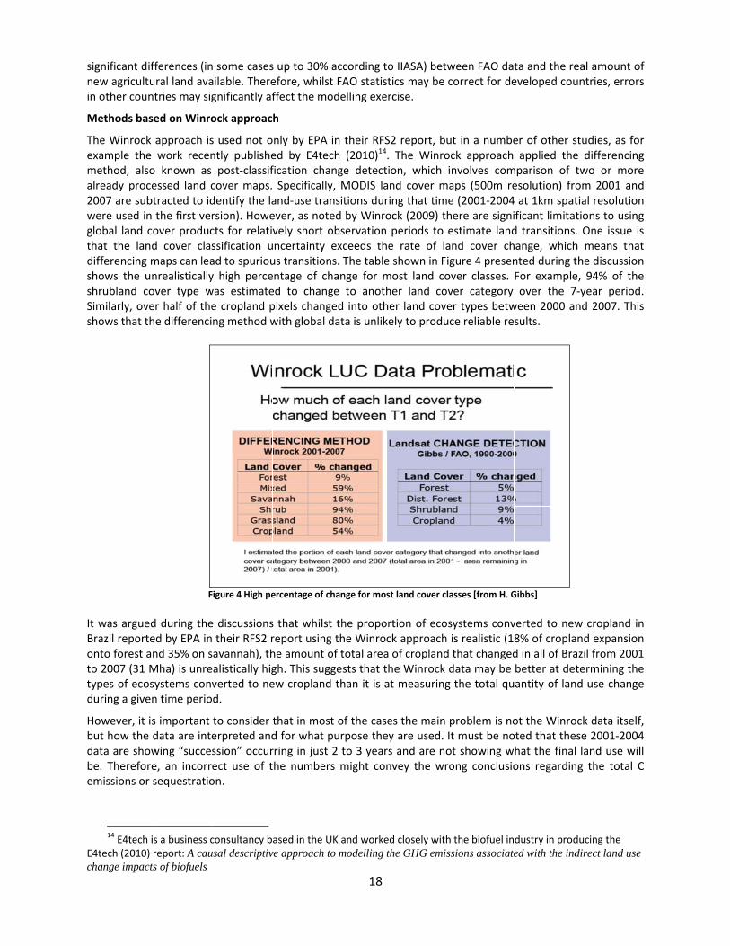
The Winrock example  the method,  alsoalready proce2007 are subwere used inglobal  land chat  the  landifferencing mhows  the  uhrubland  coSimilarly, ovehows that th

 

 t was arguedBrazil reporteonto forest ao 2007 (31 Mypes of ecosduring a give

However, it isbut how the data are showbe.  Thereforeemissions or 

                 14 E4tech i

E4tech (2010) change impact

fferences (inural land avantries may sig

sed on Winro

approach  iswork  recen

o  known  as essed  land  cbtracted to id the first vercover producd  cover  clasmaps can leanrealisticallyover  type  wer half of thehe differenci

F

d during theed by EPA innd 35% on sMha) is unresystems convn time perio

s important data are intewing “succese,  an  incorrsequestratio

                      is a business creport: A cau

ts of biofuels 

n some casesailable. Theregnificantly af

ock approac

s used not ontly  publishepost‐classif

cover maps.dentify the larsion). Howects  for  relatissification  uad to spuriouy  high  percewas  estimatee cropland png method w

Figure 4 High pe

e discussions their RFS2 ravannah), thalistically higverted to ned. 

to consider erpreted andssion” occurect  use of  ton. 

                     consultancy busal descriptiv

s up to 30% aefore, whilstffect the mo

h 

nly by EPA  ied  by  E4tecfication  chan  Specificallyand‐use tranever, as notevely short ouncertainty  eus transitionsentage  of  ched  to  changpixels changewith global d

ercentage of ch

s that whilst report using he amount ogh. This suggew cropland 

that in mostd for what prring  in just 2the numbers

ased in the Uve approach to

18 

according to FAO statistidelling exerc

in their RFS2ch  (2010)14. nge  detectio, MODIS  lannsitions durined by Winrocobservation pexceeds  thes. The table sange  for moge  to  anotheed  into othedata is unlike

hange for most

the proportthe Winrock

of total area ogests that ththan  it  is at

t of the casespurpose they2 to 3 years s might  conv

K and workedo modelling th

 IIASA) betwics may be cocise. 

2 report, butThe Winrocon,  which  innd  cover mang that timeck (2009) theperiods  to e  rate  of  lanshown in Figost  land  cover  land  coveer  land coverely to produc

t land cover cla

tion of ecosyk approach iof cropland te Winrock dt measuring 

s the main py are used. Itand are notvey  the wro

d closely with he GHG emiss

ween FAO datorrect for de

t  in a numbeck  approach nvolves  comps  (500m  re (2001‐2004ere are signistimate  landnd  cover  chgure 4 presenver  classes. er  category r types betwce reliable re

sses [from H. G

ystems convs realistic (1that changeddata may bethe total qu

problem is not must be not showing wong  conclusio

the biofuel insions associate

ta and the reeveloped cou

er of other sapplied  the

mparison  of esolution)  fr4 at 1km spatificant limitad  transitionshange,  whichnted during tFor  exampleover  the  7

ween 2000 asults. 

 Gibbs] 

verted to new8% of croplad in all of Brabetter at deantity of  lan

ot the Winrooted that thehat the finaons  regardin

dustry in proded with the ind

eal amount ountries, erro

studies, as foe  differencintwo  or morom 2001 antial resolutiotions to usin. One  issue h  means  thathe discussioe,  94%  of  th7‐year  periond 2007. Th

w cropland and expansioazil from 200termining thnd use chang

ock data itseese 2001‐200l  land use wng  the  total 

ducing the direct land us

of rs 

or ng re nd on ng is at on he d. his 

in on 01 he ge 

lf, 04 will C 

se

19  

Economic projections relying on CET functions 

GTAP‐based  models  don’t  include  unmanaged  land,  (they  only  consider  MANAGED  forest  converted  to cropland),  and  the  CET  function  used  is  based  on  comparing  land  rents.  This  is  because,  within  a  CET framework  the new  land has  to come  from an economically valued source  (an economic  trade‐off between managed  forest  and  cropland).  Therefore,  about  40%  of  the World’s  forest  is  not  included,  because  it  is unmanaged  and  has  thus  no  rent.  This  not  only  gives  an  underestimation  of  the  potential  for  forest conversion, but also prevents the capture of the whole economic pathway leaving out large sources of forest land.  Timber products  in GTAP  for  example  can only be provided by  converting  agricultural  land back  into forest,  because  any  new  forest  cannot  be  cleared. Moreover,  CET  functions  are  empirically  derived,  but because all the data are based on recent US experiences, and extrapolating economically driven LUC from CET functions for other countries might then be questionable.  

2.1.3DriversforextralandallocationTo guide the allocation process models generally consider land price, maps of land suitability, and proximity to transport infrastructure, existing cultivation and processing plants. When  discussing  the  capability  of  present  methodologies  in  capturing  land  use  changes  and  correctly allocating the changes, it is not relevant to identify what is driving the demand (e.g. whether it be biofuels or soybean consumption  in China or beef consumption in Europe). The key question is what  is really driving the allocation of cropland changes. Land suitability  is certainly one driver (it  is one of the criteria used  in the JRC methodology (JRC, 2010c)), but other socio‐economic criteria and political constraints on  land use  in specific countries  are  also  important.  These  criteria  are  generally  not  included  in  models;  particularly  in  purely biophysical models (like CLUE15 for the EU) that fail to account for political constraints on land use. In  Indonesia  for example,  land suitability, socio‐economic criteria and proximity  to existing cropland are not always the main criteria driving LUC. What matters more are the administrative boundaries, how easy it is to obtain  the  land  for  cultivation  and  the  ownership  (the  land with  the  least  ownership  claims  can  often  be obtained more easily).However, in most cases from an environmental perspective this also corresponds to the least suitable land, since in Indonesia this often happens to be land on peat. In cases like this, the use of good historical data may be able to more accurately determine the most likely areas for future land conversion.  

2.1.4ExclusionofprotectedareasfromavailableareasIn  some  regions  governmental  programmes  are  increasing  native  protected  areas:  It was  reported  that  in Brazil at present there are 108 Mha of native protection areas and indigenous reserves in the Amazon (out of a total land area of 400 Mha). The Brazilian Government is also setting up national parks in the Cerrado region, thereby reducing deforestation in this area by 40%. It was  indicated  by  PBL  that when  the  LEITAP model was  run  for  a  global  increase  in  protected  areas  of between 17 and 20 % there was little effect on the land prices in land abundant regions such as Brazil (thus a weak effect on the land conversion). LEITAP has regional land markets, and in reality the effect may be larger because the areas protected may be the most likely to be converted. The most  likely effect of  increasing protection of forests will be a shift of deforestation to other regions. For example protecting only 20% of Amazonia in Brazil will move the deforestation elsewhere. It was shown that a similar shift has already occurred in Indonesia, where a 15% increase of protected forest shifted deforestation to Myanmar and Cambodia. Some economic models are already excluding protected areas,  for example: FAPRI excludes protected areas from agricultural  land availability  in  its Brazilian module. LEITAP  takes  into account current protected areas using data from International Union for Conservation of Nature (IUCN).  

No protected area constraint  is  included  in  IFPRI‐MIRAGE, but  IPFRI agreed that  if this constraint were to be introduced in a CGE model the land availability would be reduced. In some regions there may be sufficient land 

                                                            15CLUE (Conversion of Land Use and its Effects Modelling Framework) is a dynamic, multi‐scale land use and land 

cover change model. http://www.cluemodel.nl/ 

ad

Itcc

Ite 

AaFepdr F

AFstyfa(s2fb 

 ScvtbAu

w

 

available  for demand in 20

t was pointecalculate  landcase for the e

t  is  importaestimates. 

2.1.5As discussed and the propForests  contaexpansion  is proportions  odifferent  lanegionalized e

Fraction of cr

A recent pubFAO  data  froubjected to ypes producallow agricusummarized2000 more throm disturbeby the JRC Tr

Some of the cropland andviable econohe only validbehaviour caAnother probunderestimat

                 16FAO and

world and the 

expansion, 020 is pushin

d out that wd suitability economic mo

nt  to  know

5Landconabove a keyortion of neain  higher  ccritical to ILof  different d  uses  leadestimates. 

ropland on f

lication fromom  120  samcomplemenced by  FAO lture,  theref in Figure 5) han 55% of ed forests. Topical Resou

main limitatd pasture clamic tools  fod alternativennot be exclblem relatedtions  of  for

                      d the JRC are jresults will be

but  in specing cropland i

whilst exclusiofor  the convodels that us

  the  C  stoc

nversiony issue in estw cropland tarbon  stockLUC emissionland  cover 

d  to  remark

forest in the 

m Holly Gibbsmple  sites  (ptary analysisfor  these  imfore providinshowed thanew agricultThe FAO resuurces and Env

Figure 

tions of the sasses are aggr predicting e  to have  ‘reuded.  to the identrest  convers

                     ointly workinge ready in 201

fic areas  thiinto many re

on of natureversion of cse a US based

k  of  protect

timating the that will go ok  than  otherns. Satellite  ibeing  convekably  high  in

tropical are

s et al. (2010published  bys of their satmages  also  ing  informatiat in the samtural  land  inults are also vironment m

5 Sampled are

study are thagregated, anwhere the ealistic’  indic

tification of tsion)  is  tha

g with a new 11, 

20 

is constraintegions, so ma

 protection aropland  (e.gd CET functio

ted  areas  as

emissions fronto forest (r  land  coversmages fromerted  to  cronconsistency

as 

0) was presey  FAO  in  thtellite imagencluded  cateion about  th

mpled areas (crease  is creconfirmed bmonitoring by

eas in the tropic

at  it covers nd  the data new croplancations abou

the amount oat  in  some 

bigger sample

 will be actiarginally nat

areas is be ag. LEITAP or on for contro

s  this  can  s

rom ILUC is tand in conses,  so  the  pr

m different yepland. Howey  between 

nted by JRC he  Forest  Reery with a higegories  relathe use of defor the tropieated from  iby the analysy Satellites p

cs (from Gibbs 

only about 1are  limited  tnd  is going tut  the  trends

of forest concases  prim

e of land beyo

vated. Moreure protectio

pplicable forthe  JRC metolling all wor

significantly 

to identify thequence ontoportion  of ears are ofteever,  the  difmaps,  and 

co‐authors oesource  Assgher resoluttive  to permeforested arics) historicantact forestssis of the Lanproject (TREE

et al., 2010) 

10% of foresto the 1980o come  froms, although 

nverted to crmary  forests 

ond tropics, co

eover,  the  inon will play a

r models thathodology)  trld land use c

affect  the  I

he type of lao shrubland forest  used

en used to refficulties  in thus  high  u

of the paper.sessment  fotion (30x30mmanent/smaleas. Results ally between s, and anothndsat databaES). 

sted areas ins and 1990sm, historical deviations  fr

ropland (andhave  been

overing also th

ncreased  fooa role. 

t are trying tthis  is not  thchange. 

LUC  emissio

and converteand pasture

d  for  croplanegionalize thdistinguishinuncertainty 

. In this studr  2000)  werm). Land covellholdings  anof  this  studthe 1980 anher 28% camase develope

 

 the tropics1

s. But with ndata remainrom historic

 which causen  deliberate

he rest of the 

od 

to he 

on 

ed e). nd he ng in 

y, re er nd dy nd me ed 

16,  no ns al 

es ely 

rO 

F

AHrcItbWpinn F

Utt

 

Itddgdttyfcp

gs

t

 

eclassified aOil palms). 

Fraction of cr

According to However, it wate of abandcase, then tht should be sbeing convertWhen makingplantations, an  the  IFPRI‐necessarily m

Fraction of p

Undrained  phoroughly dhrough oxida

t  was  arguedrainage  accdensity,  thusgrowth. Withdecompositiohe available hat  the  incryears. This leive years  is ccarbon  emispeatlands,  co

                 17 In this c

going onto abaequestration 

18 The Trohe Malaysian 

s secondary 

ropland on f

modelled rewas argued tdonment of ae loss of carbstressed thatted to croplag a shock onand thereforMIRAGE  bas

mean cutting 

alm on peat

eatlands  arerained, with ation, the pe

Figu

ed  by  the  Tcompanied  bs  improving h  compactioon and peat scientific stuease  in bulkeads to the ccaused almosions.  It  waompared  to 

                      case, to calculaandoned land

pical Peat ResPalm Oil Boar

(managed) 

forest in the 

esults, part othat the  incrarable land ibon stock wit, at least foand. This is b 1st generatre cropland wseline  for  thexisting fore

t 

e  a  significathe resultingeat that then

re 6: carbon em

Tropical  Peatby  water  coon  the  capion  and wateoxidation acudies give evk density moconclusion thost entirely bas  argued  thconditions 

                     ate the GHG b, bringing this

search Laborard and other E

forests, thus

EU 

of the  increarease of demn the EU (i.eill be the carr the GTAP bbecause thestion biofuels,will be taken he  EU,  expaest. 

nt  carbon  sg impacts: dn becomes a 

missions from p

t  Research ontrol  (comllary  rise wher  control,  ttually decreavidence of thostly occurs hat the subsby peat oxidhat  this  domin  temperat

balance of usis land back to 

atory is a reseaE‐science fund

21 

s becoming 

ase  in  land umand for EU e. land will bebon that wobased modese models on, cropland prfrom plantansion  of  for

sink  but  to  srainage lowecarbon sour

 

peatland draina

Laboratory paction  andhile  also  incrhe moisturease. This is chis practice. in  the  first idence rate dation not cominance  of e  peatlands

ng abandonedcultivation fo

arch division edings.  

‘suitable’ for

use  in the EUbiofuels croe recovered uld have accls, “deforestnly include corices will incations or fromrest  plantati

support  palmers the waterce (Figure 6)

age [presented

(TPRL)18  repd  water  manrease  the we  content  ofertainly the Moreover, dfive years afof around 5 ompaction, aoxidation  a,  is  due  the

d land, one shor crops will le

established by

r the cultivat

U will still coops may be mfrom abandocumulated oation” only rommercial forease compam a reduced ons  are  exp

m  oil  produr table, dryin). 

d by A. Hooijer,

presentative nagement) ater  filled pf  the  peat  inideal situatiodata presentfter drainagecm yr‐1 thatand therefors  a  cause  o difference 

hould also conead to a  loss o

y the Sarawak

tion of speci

me from “demet by a redoned land) 17

n the idle lanrefers to maorest plantatared to the vincrease of fpected  ,  so 

uction  peatlang and thus d

, Deltares] 

from  Malawould  increore  space  foncreases  anon, but at prted by other e, and  is mit still occurs re correlatesof  subsidencin  temperat

nsider that if aof foregone ca

k government

ific crops (e.

eforestationduction  in th7.  If this is thnd.  naged forestions. value of foreforest. In facthis  does  no

ands must  bdecomposin

 

aysia  that  thease  the  buor good pland  the  rate  oesent none oexperts shonimal  in  lateafter the firs directly witce  in  tropicture of  near

afforestation iarbon 

 and funded b

g. 

”. he he 

ts 

st ct, ot 

be g, 

he lk nt of of w er st th al rly 

is 

by 

2s

TIninF

 

A(b

 

Int(p22a

im

 

20oC. Studiesoil temperat

The main  regndonesian pn global tropFigure 7).  

Although  it  isFigure 8), sobecause of th

Figure

n Indonesia hat by 2025 unofficial logpalm covered2009” showe2007). The TPand Indonesi

                 19 Wong, J

mpact of biofu

s  in the Everture, at an ev

gions  affecteeatlands arepical peatland

Figure 7: glo

s evident  thources disagrhe different d

e 8: compariso

at present aoil palm andgging may cad 0.31 millioed that land iPRL represena is lower th

                      J., Presentatiouels policies o

rglades (USAven water de

ed  by  peat e likely to conds, estimate

obal distributio

at a  large  frree on the exdefinitions o

n of 1980 and 2

about 5.5‐6 Md pulp woodause additionn ha (9.5%) oin Malaysia untative claiman those rep

                     on made by thon tropical def

A) have showepth. 

conversions ntain 84% ofd at 89 billio

on of peatland 

raction of oixact fractionf “peatland”

2007 land use mSarawak19pr

Mha of peat plantations nal significanof total peatused for oil pmed that the ported (respe

he Forestry Deforestation in 

22 

wn that the r

are  Indonef the entire Con tonnes (no

areas and C sto

l palm and a of existing o”.  

maps for Sarawresented by H.J

tland are estwill cover m

nt drainage).tland area wpalm increasfraction of pectively 5% i

epartment of SMalaysia”, Ku

rate of peat 

sia  and MalC in tropical ot including 

ore [presented

agricultural oil palms tha

wak region (MaJ.Stibig – JRC)

timated to bmore than 50FAOSTAT da

which rose to sed from 0.2 peatland usen Malaysia a

Sarawak, JRC‐uala Lumpur, 2

oxidation do

aysia,  and opeatlands inthe biomass

d by S. Page – U

area movedat is on peat

alaysia) [Source

e used for o0% (10 Mha) ata for Malay0.51 millionmillion ha in

ed for oil paland 15% in In

‐MPOC works20‐22.Nov.20

oubles with 

on  the  basisn SE Asia ands of 69 Billion

 Univ. of Leiceste

d onto peat sland. In som

e: Forestry Dep

oil palm. Projof peatlandysia shows thn ha (13%) inn 2003 to 0.6m plantationndonesia).  

hop on “Direc008 

every 10oC 

s of C  storagd 65% of the n tonnes) (Se

er] 

swamp  foreme cases this 

partment of 

jections shos in Indoneshat in 2003 on 2008 (“TPR6 million ha ns in Malays

ct and indirect

in 

ge C ee 

st is 

 

w ia oil RL, in ia 

t 

23  

3.GHGemissionsfromLandUseChanges

This section focuses on whether the available datasets are adequate to calculate ILUC emissions and if all the relevant parameters are effectively considered by the different methodologies. 

3.1MethodologiestocalculateGHGemissions The IPCC methodology is the most commonly used method to calculate GHG emissions due to LUC.  

A complementary approach consistent with  the method used  for  the assessment of biodiversity  in LCA was also discussed. The Global Warming Potential (GWP) index proposed by the IPCC for assessing the contribution of different GHGs to climate change was not designed for application  in LCA and  is based on subjective time preferences. Instead, the approach of Müller‐Wenk and Brandão (2010)(presented by J. Reinhard from EMPA) is consistent with the GWP index and with the method used for the assessment of biodiversity in LCA. This method, based on Moura‐Costa (2000), derives an equivalence factor between tonne C‐eq. and tonne C‐year.  This  factor  is  applied  to  biogenic  carbon  emissions  from  land  and  assessed  against  their  fossil counterparts. The difference results  from the different residence times  in the atmosphere that arises. When land‐use  change  (LUC)  takes  place,  the  carbon  stored  in  soils  and  biomass  is  released.  By  doing  so,  an additional  sink  is  concurrently  opened  on  that  land which  is  able  to  retrieve  back  the  carbon  emitted.  In consequence,  one  tonne  of  C  from  LUC  has  a  different  impact  than  one  tonne  of  carbon  from  fossil  fuel combustion. The advantage of applying this methodology to LCA is that it considers not only carbon quantities transmitted to the atmosphere but also the mean duration time of these carbon quantities in the atmosphere. Furthermore, it is in line with the current LCA methodology to assess biodiversity impacts.  Some  criticisms were  raised on  the possibility of  the  LCA methodology  in particular, double  counting  the C sinks: it was in fact argued that the LCA method assumes that the cropland re‐grows, and that the re‐growth of a forest counts as a C sink. If the land is converted to cropland then the C should count the same or if the land is converted to cropland and the model assumes that there is re‐growth of forest elsewhere (which happens in the GTAP model) then the C will be counted as a sink separately. If you have already accounted for that, you will  be double  counting. Most  of  the  LUC models  (e.g.  IFPRI‐MIRAGE)  assume  that  the  land  use  change  is permanently converted to cropland. The  IFPRI‐MIRAGE model  looks at the amount of  land by activities  (e.g. cropland managed  forest etc.) and assumes  a C  value  for each of  these  land  types.  (In  the  report by  IFPRI (2010), it was assumed that in the EU the forest lost was new forest (from afforestation) which has half the C of a mature forest). However,  the  authors  of  the  discussed  methodology  argued  that  even  considering  land‐use  change  as irreversible  (quite a strong assumption),  the  impacts of  land use  (i.e.  land occupation) are attributed  to  the current crop and not to the crops that originally triggered the  land‐use change. So,  if  it  is only the triggering crop  (i.e. biofuels)  that you’re assessing, you  can only ascribe  it  the  transformation, but not  the  ‘unknown’ subsequent occupation impacts  Time: Amortization over 20 years 

In  all  cases  results  depend  on  the  amortization  period  (the  EU  legislation  decided  to  go  for  20  years  as specified under the Tier 1 approach of IPCC, while US legislation goes for 30 years). It was argued  that  for policy comparison an appropriate discount  factor must be chosen.  It  is  important  to understand that the time profile of LUC emissions (which are added to the direct emissions from biofuel use) is different from the time profile of the same amount of C emitted by fossil fuels. There is no discount factor in the LCA methodology and the claim  is that there  is no difference between a C discharge now and 500 years from now.  In  response  it was noted out that the  (Publicly Available Specification) PAS 2050 British standard (2008) does account for delayed emissions.  

 An understanding of the change in the long term situation beyond 2020 is also important for the sustainability criteria of biofuel production. 

24  

3.2AccountingforforegoneCsequestrationProper estimations of  ILUC emissions must  also  account  for  carbon  sequestration, which has proven  to be difficult  to  accurately  assess. Most  of  the  studies which  estimated  low  ILUC  emissions  by  allocating  large amounts  of  cropland  to  abandoned  land  for  example  did  not  properly  account  for  the  foregone  C sequestration  when  the  land  is  cultivated  again.  The  main  issues  identified  during  the  discussions  are summarized below.  1. Carbon sequestration due to afforestation 

The rate of carbon accumulation on abandoned arable land is entirely different from the amortised carbon loss from  deforested  land  and  grassland.  It  depends  on  whether  land  is  left  idle  (natural  succession)  or  is afforested.  According to FAO data, 1,134,000 ha of land has been abandoned between 1995 and 2005 in the EU, of which 721,000 ha has been reforested. The E4tech (2010) study presented at the meeting applies afforestation gains to only 12% of these abandoned  lands (138,000 ha), and calculates Soil C stocks on 88% of this  land, without considering  the  amount  of  afforestation  on  active  cropland.  It  was  argued  at  the  meeting  that  this underestimates the area afforested and hence foregone C sequestration.  

The table shown  in Figure 9 gives the range of afforestation and the rate of C accumulation associated with foregone sequestration in the EU that are assumed by different models.  

 Figure 9: Afforestation rates in the EU assumed by different models [presented by W. Lywood – Ensus]. 

However,  it was pointed out  that  some  studies  (e.g.  E4tech,  2010)  do not  take  into  account belowground biomass in estimating GHG Emissions.  . For example, the accumulation rate of 0.48 t C ha‐1 yr‐1 reported in the figure above is just soil C from natural regeneration. Therefore,  it  is necessary to add vegetative carbon  (~1.75 t C ha‐1 yr‐1.) thus bringing the total closer to 1.5‐ 2 t C ha‐1 yr‐1, while for plantation forests the C accumulation figure is closer to 2.5 to 3.5 t C ha‐1 yr‐1 20.  

 2. Misinterpretation of Winrock reversion factors (afforestation) 

In  addition  to  estimating  emission  factors,  Winrock  International  also  developed  “reversion  factors”  to estimate the carbon accumulation in biomass and soils that occurs when managed cropland and pasture land is  abandoned,  looking  at  re‐growing  forests  and  forest  accumulation  rates. However,  the  correct  use  and interpretation of these reversion factors has been proven to be critical for a number of reasons: 

 ‐ The calculation of potential  losses of C sequestration  is  largely underestimated  if average sequestration of mature  forest  is  used,  and  not  the  re‐growth  of  freshly  planted  forest  (as  should  be  the  case  in  EU  for abandoned land). 

‐ Winrock identifies the new use of land in 2006 that was cropland in 2001. This time period is not sufficient for forest to form a significant canopy cover. So the new forest growth viewed from the MODIS satellite does not 

                                                            20 Searchinger, 2010. Technical note “Comments on draft ILUC analysis of rapeseed and palm, biodiesel presented by 

E4tECH in February 2010”. Available on‐line at http://www.endsreport.com/docs/20100428b.pdf 

Carbon stock change for converted cropland in the EU

Model Method C stock change Sourcet C/ha/yr

Analysis of historic data FAO 0% 0.48 Lywood 2010E4tech reversion MODIS 45% 1.5 E4tech 2010E4tech conversion MODIS 6% 1.7 E4tech 2010IFPRI Cost curve 34% 1.9 IFPRI 2010JRC new methodology AEZ etc 38% 1.7 JRC 2010cGTAP CET 77% 3.4 JRC 2010b

% of new cropland

from forest

25  

show  up  as  forest,  but  as  one  of  the  “intermediate”  categories  such  as  savannah,  scrubland  or  “mixed” (totalling 67% of the land reversion) or even as grassland. That is why the study from E4tech (2010) discussed during the meeting reported only 6% reversion of cropland directly to forest. 

‐  It  is clear  that  satellite data cannot  show  clearly new  forest growth  in only 4  to 7 years and  the  land‐use reported by Winrock after just 5 years reversion is not the final land use which should be used to calculate the C stock change. Therefore using  this  information on  intermediate  land‐cover classes as  the  final  land‐cover, systematically  underestimates  the  amount  of  new  forest  which  is  growing  and  the  foregone  carbon sequestration from increased EU crop area.  

‐ For a mistake  in the datasets published by Winrock  International, the coefficients  for carbon accumulation (change  in biomass C stocks) for reversion of EU  land to forest were accidentally set to zero (for comparison, the  values  assumed  for C  accumulation on US  re‐growing  forest  is 9  t C ha‐1  yr‐1). Therefore,  the  foregone carbon  sequestration was  largely underestimated  (roughly a  factor of 3)  for  the  studies  (e.g. E4tech, 2010) which made  use  of Winrock  coefficients  to  calculate  the  carbon  stored  in  re‐growing  EU  forests  –  e.g. on abandoned land. 

EPA also used Winrock coefficients, but having realized the above problems, when a natural reversion was occurring in one region, instead of applying Winrock reversion factors they looked at the proportion of land cover in that region (land cover in 2007) and used the annual biomass growth to calculate the reversion of carbon. For example, in a region that was 80% forest, it was assumed that 80% of abandoned agricultural land would grow back as forest.  

3.3GHGemissionsfromdrainingpeatlandsCarbon emissions from peat oxidation can be measured in two ways: by direct measurements of carbon fluxes on  site  (mostly CO2,  sometimes CH4),  and by monitoring  the  subsidence  level  and determining  the  relative contribution of oxidation (decomposition and mineralization). 

1. GHG flux measurements on peatland are costly and complicated and thus the results are limited. Moreover, it was  noted  that many  studies  have  not  separated  root  respiration  emissions  (natural  cycling  of  C)  from emissions  due  to  oxidation  (caused  by  drainage)  and  none  of  the  studies  provide  the  full  C  balance.  CO2 emissions  calculated  through  flux measurements  vary  considerably,  ranging  from  below  40  tCO2  ha‐1  yr‐1 [Melling et al, 2005, Muruyama and Bakar, 1996] to well above 70 tCO2 ha‐1 yr‐1  [Hoojier et al., 2006, 2010; Couwenberg et al., 2010]. These GHG flux measurements are best used as an independent check on the results of other methods. 

2. The best alternative method to assess peat emissions is by subsidence modelling. Most of the studies show that 75% of subsidence is oxidation, and this can be measured as CO2 emissions.  

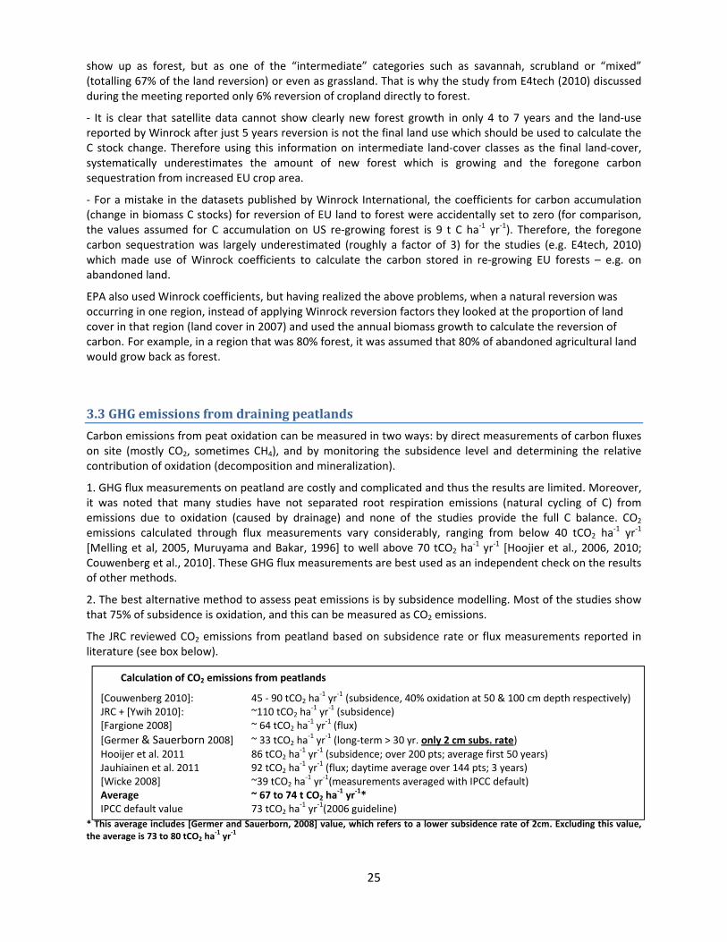
The  JRC  reviewed CO2 emissions  from peatland based on subsidence  rate or  flux measurements  reported  in literature (see box below). 

 

 

 

 

 

 

 

* This average includes [Germer and Sauerborn, 2008] value, which refers to a lower subsidence rate of 2cm. Excluding this value, the average is 73 to 80 tCO2 ha

‐1 yr‐1 

 

Calculation of CO2 emissions from peatlands

[Couwenberg 2010]:  45 ‐ 90 tCO2 ha‐1 yr‐1 (subsidence, 40% oxidation at 50 & 100 cm depth respectively) 

JRC + [Ywih 2010]:   ~110 tCO2 ha‐1 yr‐1 (subsidence) 

[Fargione 2008]   ~ 64 tCO2 ha‐1 yr‐1 (flux)  

[Germer & Sauerborn 2008]   ~ 33 tCO2 ha‐1 yr‐1 (long‐term > 30 yr. only 2 cm subs. rate) 

Hooijer et al. 2011   86 tCO2 ha‐1 yr‐1 (subsidence; over 200 pts; average first 50 years) 

Jauhiainen et al. 2011   92 tCO2 ha‐1 yr‐1 (flux; daytime average over 144 pts; 3 years) 

[Wicke 2008]   ~39 tCO2 ha‐1 yr‐1(measurements averaged with IPCC default) 

Average  ~ 67 to 74 t CO2 ha‐1 yr‐1* 

IPCC default value   73 tCO2 ha‐1 yr‐1(2006 guideline) 

TSbF

 

Tli“eaemTpytfeC(ees

 

The  subsidenSauerborn, (2by oxidation Florida Everg

 

The  IPCC defimit  if we  e“coincidence”emissions  froagriculture vaet  al,  2011, measuremenThese studiesplantations, ayears since dCO2 ha‐1 yr‐1,ind  92  tCO2

emissions froConsidering  aequivalent  testimations, hould be dis

nce  rate  is 2008) emissiof tropical plades. 

Figure 10: p

fault value  foxclude  [Ger” does not mom  oil  palmalue should Jauhiainen  ents “in‐situ” as show relatand suggest drainage  (see, and annual2  ha‐1  yr‐1.  Tom non‐plantall of  the abto  73  tCO2 and  its  appscouraged in 

expected  toons are basepeat must be

peat subsidenc

or agriculturmer  and  Samean that thm  plantationbe used rathet  al,  2011] and providinions betweecarbon loss e Figure 11  ,lized over 50These  valuestation areas bove,  the emha‐1  yr‐1)  slication  in  efavour of th

o  be  4‐6  cmed on 2 cm oe about 60%

ce level [presen

re  in the trouerborn,  20he IPCC valuns  on  peatlaher than thewere  preseg more robuen water depof at least 7, combined w0 years it is 8s  are  still  exaffected by mission  factohould  be  coestimating COhe more appr

26 

m  per  year  iof subsidence(Cowenberg

nted by A. Hooj

pical peat  fa008]  value,  fe for agriculands  (for  exe managed foented  at  theust estimatespth / subside70 tCO2 ha‐1

with Figure 86 t CO2 ha‐1

xcluding  emplantation dor of 20  tC onsidered  aO2  emissionsropriate emp

n  SE  Asia,  ae rate only). g et al, 2010

jier, Deltares]

alls  in the rafor  the  reasoture on peaxample,  it  isorest value).e meeting,  bs of the emisence / carbonyr‐1 at aroun10 above).  Iyr‐1. Concur

missions  due rainage.  ha‐1  yr‐1propas  a  still  cos  from oil ppirically‐base

as  shown  inIt was show), while it is 

nge of averaons  explainet  is the moss  not  unam Rather, mobased  on  emssions factorsn loss in Sumnd 70 cm wan the  first yrent CO2 fluxto  fire,  bio

posed by  thenservative  fpalm plantated values. 

n  Figure  10.n that the frapproximate

 

aged values ed  above).  Hst appropriatmbiguously  cre recent stumpirical  obses. matran oil paater depth afyears this  is wx studies at tomass  loss  a

e  IPCC  in 20factor  for  Gions on  trop

  Germer  anraction causeely 75% in th

(at the  loweHowever,  thte to estimatclear  that  thudies [Hooijeervations  an

lm and acacfter the first well over 10the same siteand  oxidatio

006 guidelineGHG  emissiopical peatlan

nd ed he 

er his te he er nd 

ia 5 00 es on 

es on nd 

 WgCdmyc 

 

Tas

 

Figure 11: E

Whilst uncertgreater uncerCO2 Emissionduring clearinmust be also yr‐1,  and  althcertainly ther

The  above  eaccounted  foequestration

Emissions from

tainties in emrtainty in idens from canang should alsconsidered: hough  therere is an impo

Figure 12: Fi

emissions  (for  in  most n is shown in

m peat oxidatio

missions fromentifying the l digging/dreso be includeannual C los

e  are  uncertortant correla

ire map (2010) 

from  fires, of  the  calcn Figure 13. 

n as a function

m tropical peland uses onedging and Ced. In additiss due to peatainties  on  hation, as from

and forest ma

canal  digginulations.  An

27 

n of water dept

eatland haven peat. CH4 emissionon, annual Catland fires ihow much m Figure 12

p (2007) in Sum

ng  etc.),  incn  estimate  o

h [presented b

e been largely

ns from canaC loss due ton South Eastcan  be  attrbelow. 

matra [presente

cluding  reduof  the  mos

by A. Hoojier, D

y reduced in

l bottoms ano peatland firt Asia is estimibutable  to 

ed by S. Page, U

uced  carbont  likely  valu

 Deltares] 

 recent year

nd biomass lres as a resumated to be plantation 

 Univ. of Leicest

n  sequestratues  for  loss

rs there is 

loss emissionult of drainagabout 191 Mdevelopmen

ter] 

tion,  are  noes  in  Carbo

ns ge Mt nt, 

ot on 

 TprdWmtwdtTouoc

3 

L

Itus

Itiddbrin

 

Figure 13

Tropical Peatpeat.  Therefoeported.  Trodistinct from When speciamay be reduhe order of 7water levels adifficult to ashe bulk densThe general conly becauseundrainable iof tropical peconclusion, u

3.5Adequa

Land availabi

t  is  importaunderestimattocks. 

t was showndentify chandata  it is not being converesolution dan the near fu

: Reduction of use ch

t Research  Lore,  the diffopical  peat the previoul attention isced (but thi70‐100 cm inare). In any cssess the aresity). conclusion ise of the carbin the longereat swamp  fnderlying th

aterepres

ility in satell

nt  to  underting  land  av

n that the lownges  in  land possible to 

rted to oil paata (such as uture when t

C sequestratiohange on South

Laboratory  rferent  types differs  in  cos. s paid to coms occurs onln Indonesia (case the IPCCeas of peatla

s that peatlabon emissionr term (betwforest  into aat also socia

entationo

lite data 

rstand  if  datvailability wi

w resolutionuse and thuidentify  impalm plantati30 m) whichthe results of

n and C releaseheast Asian pea

eported  thaof peat wil

omposition  f

mpaction of ty on  limited(the target isC value for trand, how mu

nds are not ns, but also bween 25 and gricultural aal and econo

oflandava

tasets  (e.g. ll  affect  bot

n of satellite s difficult toportant land ons. To  idenh at present f an FAO – JR

28 

e due to peat oatlands [presen

t much of  tl  influence  tfrom  peat  fo

the peat, thed areas).The s lower in Mropical peat uch C  is stor

suitable or sbecause of t100 years), area. The repmic develop

ailability(e

FAO, MODISth  the  estim

data (e.g. Mo estimate house changesntify these cis not availaRC Global sam

oxidation and cnted by S. Page

the  researchthe decompormed  by  sp

e rate of sublevel of peaalaysia, aboconversions ed (which d

sustainable fthe  inevitabiand for the lopresentative ment should

e.g.CISand

S)  are  accurmation  of  lan

MODIS 250 mow much  lans such as nahanges  in  lable globally.mpling surve

combustion asse – Univ. of Leic

 on peatlanosition  rate phagnum  an

sidence (andatland drainaut 60 cm, budoes not coepends on t

for agricultulity of manyoss of biodivof TPRL how

d be consider

dEU)

rately  showind  conversio

m land cover nd  is availabtural forest and cover wo. However, sey are releas

 sociated with acester] 

d  is based oand  the ox

nd  reaction  t

d therefore tage  is also  imut it is uncleansider deep he depth of

ral productioy of these areversity linkedwever disagrred. 

ing  land  avaon  and  the 

data) makesble. Notably,(e.g. peat swould requiresuch data wied. 

ll forms of land

on  temperatidation  leveto  draining 

the emissionmportant:  it ar what actudrainage. It f the peat an

on. This is noeas becomind to the switcreed with th

ailability  sincimpacts  on 

s it difficult t using MODwamp foreste much highell be availab

d 

te ls is 

s) is al is nd 

ot ng ch his 

ce C 

to IS ts) er le 

St

 

“

FtwtAccwstdItFrE

LIncthaaT

 

Some tools ahe Geo‐Wiky

Figure

“Abandoned 

FAO statisticshat the avaiwas claimed hese lands.  Abandoned  lconverted  intcaused  by  thwetlands  in equestrationhe same as deliberately tt was noted For  exampleesponsiveneEurope. 

Lower yields n the CIS in pcan be assumhe more prohighly likely tassume that also importanThe land use 

                 21 availabl

re available y web tools o

e 14: Example o

 land” in CIS

s show that slability of thby that the i

and may be to other usehe  ending  ofCIS  have  on) and wouldland set‐asidtaken out of that that me:  Partial  eqess  of  produ

on abandonparticular, yimed that mooductive  landthat the increextensificatnt to understhas still chan                      e at geo‐wiki.

to help the voperated by 

of IIASA geo‐W

S and EU 

since the 19his abandoneincreased de

defined as es for many f  state  subsoften  been d be unlikelyde in the EU production tany of the mquilibrium  muction  and  t

ned land ields on abanost of the  lesd has been kease will be ion  in these tand the GHnged and the                     org and agric

validation ofIIASA21(an e

Wiki tool for Com

60s croplanded  is not alwemand (for la

land that  is different reasidies,  increarewetted  ay to be convunder the Cthat has nowmodels are nmodels  havethese  elastic

ndoned landss productivekept  in prodon land whicareas will  rG implicatioerefore there

ulture.geo‐wi29 

f global land xample is sh

mparison of glo

d has been dways correctand) due to b

no  longer usasons. For  inased  labour nd  returnedverted  into cCommon Agrw come backot very goode  regional cities  would 

d are lower ce  land was tauction. Therch is less proresult  in  the ns of bringine will still be

ki.org 

cover data, fhown in Figur

obal land cover

declining in bly accountedbiofuels will 

sed as agricunstance, the costs  or  retd  to  forestcropland agaricultural Pok into producd at taking inelasticities not  captur

ompared to aken out of refore  if cropoductive, witsame yields

ng abandonee a C stock lo

forest and crre 14)  

r products [pre

both the CIS d  for  in the decrease th

ultural produabandonmeturn  of  own(to  be  use

ain. This abalicy (CAP) wction.  nto account that  are  bre  the  availa

similar regioproduction pland  is  incrth lower yiels as on presed land back ss. 

ropland stati

esented by S. Fr

and EU and agro‐econome rate of aba

uctive  land, ent of  land  inership.  Formed  in  prograndoned  landhich was agr

these structased  on  hiability  of  lan

onal climatic(i.e. abandoeased  in thods. Thereforently cultivainto back int

istics etc., e.

ritz – IIASA] 

it was arguemic models. andonment o

and has been the CIS wamerly  draineammes  for d  in CIS  is noricultural lan

tural changestorical  pricnd  in  Easter

c conditions. ned) and thaose areas,  it re, one cannoted  land.  It to productio

g. 

 

ed It of 

en as ed C ot nd 

es. ce rn 

It at is ot is n. 

30  

3.6UncertaintiesindatasetsIt was agreed that there are great uncertainties in the datasets used to calculate GHG emissions, and these are not always known. Global land cover maps are of limited use for assessing land cover conversions. The accuracy of the maps being low  (each map may have errors  that could exceed 25%)  the  risk  is  that when comparing  two maps, what  is measured is the errors in the maps, and not the change in land cover. There are alternative satellite products that do  look at  change,  (e.g.  South Dakota  State University deforestation maps with a higher  resolution of forested areas). More problematic is to find equivalent products (datasets) for agricultural areas. Winrock’s  coefficients are normally at  country  level, and within  country, but  land allocation  is at AEZ  level. Moreover in 2020 there might be no forest left in some regions and therefore country‐based historic data may no longer be realistic.  In any case reliable historical data are considered important to verify the land conversion rates, in particular in hot spots; good quality data at regional scale are available (at least for some regions as SE Asia) and need to be used rather than poor quality global data. In conclusion it was agreed that while there are uncertainties in the datasets, all indicators point towards the existence of a significant ILUC effect.    

31  

4Agro‐economicmodellinganduncertainties:This  section  focuses  on  the  lack  of  empirical  information  available, where  exactly  the models  need more information and which  important  relationships are not being modelled. There are many decisions  that have gone  into  the existing agro‐economic models  that can cause uncertainties  in  the projections. For example a single change in the underlying baseline conditions in a simulation could change the amount of biofuels being used, where  they  are being  used  and where  the  biofuels  are  being  sourced  from.  There  are  uncertainties coming  from data on  land use  change,  yields  and  fertilizers  for example, which  are  all  very  important, but underlying  these  factors  are  uncertainties  inherent  in  the  whole  modelling  exercise.  Despite  these uncertainties,  it  is  recognised  that because economics are driving  the whole  ‘ILUC’ process  the use of agro‐economic models is essential to the estimation of ILUC. Economic market models are constructed  in order  to describe and simulate national and world markets  for commodities, manufactured goods and services. When they focus on the production, market and trade flows of agricultural commodities only,  ignoring  the  rest of  the economy,  they are classified as partial equilibrium (PE) models  and  known  as  ‘agro‐economic models’. When  economic market models depict all  commodity, goods and service sectors (including agriculture), together with the interactions between them, these models are known as general equilibrium (GE) models and the name ‘economic market model’ is appropriate.  Models of both kinds are referred to in this report: for example, AGLINK‐COSIMO, CAPRI and ESIM are PE agro‐economic models whereas GTAP, LEITAP and IFPRI‐MIRAGE are GE models. Although each type of model has strengths  and weaknesses when  it  comes  to  simulating  the  global  effects of  a policy  involving  a particular group of agricultural commodities, they all share two  important characteristics. First, their prime  focus  is on markets  (behaviour  and  outcomes)  and  hence  they  are  usually  specified  at  the  level  of  aggregation  that defines  the market  (i.e.  national22).  Second,  the  underlying  driving  forces  are  those  of  rational  economic market behaviour  (e.g. higher prices  encourage  supply but discourage demand, markets  reach equilibrium, supply  is encouraged where production cost  is  low and vice versa) but they do not shed  light directly on the micro‐decision making of particular kinds of producers or suppliers, or on resource use generally. Thus, prices – not agronomic or technical possibilities ‐ play a key role in determining how and where production occurs. At the  same  time,  the  behavioural  coefficients  and  elasticities  in  these  models  reflect  a  large,  but  hidden, information  set  consistent  with  the  relevant  underlying  physical  production  conditions,  and  additional variables  (e.g.  for yield growth,  technological change) are usually  included  to allow  these conditions  to vary over  time. A  first  source of  error  is,  therefore,  the way  economic behaviour  is depicted  in  the model:  the causal economic relationships depicted and the parameters used. However, when used for their more normal tasks, users (policymakers, analysts) consider that this level of uncertainty is acceptable. To extrapolate from production decisions to  land use, each model employs  its own method, usually based  in some way on average yield  coefficients  (which allow  the  calculation of how much  land of  ‘average’ quality would have been needed to produce a given quantity). This raises the question of whether marginal yield, for a specific  crop  in  a  specific  location,  should  perhaps  be  lower or  higher  than  the  average  yield.  Clearly,  the answer depends largely on which type of land is used for crop expansion (previously cropped land – of higher or lower quality? permanent grassland, degraded land, virgin rain forest, peat land etc.23). The data required to model this  in a rigorous way are not available to the typical economic market model, and certainly not with global  coverage.  Therefore,  the  quantitative  estimates  of  land  use  change  produced  by  these models  are approximate and subject to a high degree of uncertainty. This uncertainty in the land use change estimates is transmitted to any estimates of GHG emissions based upon them.  

                                                            22Attempts have been made to regionalize some of these models: for example, CAPRI can be run with the EU 

disaggregated to NUTS 2 level (over 220 EU regions), GTAP can be linked to AEZ, a global land use model that distinguishes 18 different agro‐ecological zones.  

23Typically, economic market models do not model total land (including all its uses, commercial and non‐commercial). In general (for example, in GTAP), the total land area used for crops, pasture and commercial forestry is forced to remain constant. This means that price‐induced increases in cropland must be at the expense of pasture or commercial forests, and the depletion of rainforests or other ecologically‐valuable non‐commercial land cannot be simulated. In AGLINK‐COSIMO, ‘total land’ is land used for agriculture, and does not include commercial forestry. 

 

32  

Summarising the above, the ILUC results of these models contain various uncertainties that derive from their specification and the fact that when asked to simulate ILUC they are being pushed to the frontier ‐ or beyond – of the range of tasks they were designed to perform. All models contain an element of error (uncertainty) due to the  fact that they are stylized representations of reality. However, when used  for their normal tasks, this level of uncertainty  is usually considered acceptable. A second  layer of uncertainty, potentially far greater,  is introduced when the core model results are used to extrapolate to ILUC, using less rigorous methodology than that used for the construction of the model  itself, with  inadequate empirical content and often,  it should be added, with  inadequate behavioural  knowledge of  the  reactions of micro‐agents  in  the  real world. A  third source of uncertainty has not yet been mentioned, as it arises from the way these models are used rather than from their underlying specification. In general, in order to estimate the future effects of a policy, an economic model  is  simulated  over  a  given  future  time  period without  the  policy  change,  and  again with  the  policy change, holding everything else constant. The effects of  the policy change over  the period, or  in  the closing year of the period, are measured as the differences between the two scenarios. This means that each model exercise needs to use assumptions about the evolution of exogenous  (external) factors over the time period (e.g. GDP, population, exchange rates, technological advance, productivity (including agricultural yields) and so on24). These  choices  are  a  source of  further uncertainty,  and  can  cause differences between  the  results of different  models.  For  example,  a  simulation  study  based  on  a  vision  of  rapid  recovery  from  the  global economic  crisis  (and  hence  higher  GDP,  higher  transport  fuel  use,  higher  fossil‐fuel  prices  etc.) may  give noticeably higher  ILUC  impacts  than when more a more pessimistic outlook  is adopted. Similarly, a view of future technological and yield developments based on those observed up to the mid‐1990s will give different results from those  incorporating a more pessimistic vision  incorporating climate change‐induced  increases  in desertification and water shortages, and sluggish yield growth. This type of uncertainty cannot be substantially remedied by more data or greater understanding of the behaviour of particular agents:  it arises because the future cannot be fully predicted. The main  strength of global  (agro‐) economic models  for generating estimates of  ILUC  is  that  the  resulting estimates are  fully compatible with a consistent and detailed global view of production, consumption,  trade and prices  for the relevant commodities, and with the economic behaviour that drives these outcomes. This provides an invaluable background against which to check the plausibility of the ILUC estimates, which would be lacking in models based solely on agronomic principles. On the other hand, this strength cannot offset the considerable uncertainties in the ILUC estimates generated by these models. 

  

4.1Intensification 

4.1.1Impactofpastureconvertedtocropland 

Many  agro‐economic models, with  the  exception  of GTAP  based models,  assume  that  if  pasture  is  lost  to cropland  there  is no expansion of pasture onto  forest as  a  result. Thus  the models estimate  the minimum amount  of  ILUC  from  this  point  of  view.  GTAP‐based  models  include  knock‐on  effects  on  pasture  area indirectly by modelling economic competition for land between crops, pasture and commercial forestry.  

1. FAPRI models the competition between cropland and pasture with substitution between the two. 

2. In the LEITAP model there is substitution between the feed and the grassland used, but there is large uncertainty about the substitution elasticities. 

3. In  the  IFPRI‐MIRAGE  model  pasture  is  replaced  by  feedstock:  When  there  is  no  more complimentarity between feedstock and land you start to have substitution, which leads to potential  intensification or extensification depending on the price response of the  land vs. feedstock. With an  increased demand for agricultural crops the price of crops increase, the 

                                                            24In GE models, some of these assumptions are implicitly set by the closure rules – but choice of closure rules is, also, 

open to discussion. Typically, PE models need a larger number of quantitative exogenous projections in order to run. 

33  

price of  intermediate  inputs rise, production costs go up, demand of meat goes down and therefore  less  land  is used.  If the aggregate price of the  feedstock goes up, extensification will result, but if the aggregate price of the feedstock goes down, intensification will occur. This aggregate price depends not only on  the price of wheat or  corn but also on  the by‐products. IFPRI‐MIRAGE shows intensification in the US and EU, but extensification in Brazil. 

4. The  BLUM  model  for  Brazil  presented  by  ICONE  (and  used  by  FAPRI)  calculates  the displacement of  cattle by agricultural  crops. The model  includes pasture,  cattle  structure, and beef production, which are the main variables needed to determine the performance of the cattle sector. It was noted that the slaughter rate must also be included in the models, because  if this  factor  is not  included then the demand  for pasture  land could be under or overestimated. 

It was stated that whilst the cost of animal feed may go up as crop prices rise, some of the biofuel by‐products are used for animal feed, so the price of feed will come down. The result is that less soybean will be grown, as this  is primarily grown for the meal, and this will affect the total animal price. Therefore, to calculate the net livestock count (herd size) all the elasticities have to be accurate. 

 

Historical data and model assumptions 

To calibrate the elasticities in the models good historical data on pasture area are needed. However, many of the pasture effects are highly regional and validation of the elasticities and modelling results is often difficult, even  for  countries  like Brazil, where  regional data on  changes  in  cropland, pasture and  cattle numbers are readily available.  In  fact, agro‐economic models  simulate market behaviour and are usually  specified at  the level of  the market  (i.e. national). Some of  these models  then break down  the  results  to  the  regional  level, because many  of  the  effects  of  interest  are  very  region‐specific,  even  local,  and  this  step  is  often  a  big challenge for market‐based agro‐economic models  

The historical data used to calibrate elasticities in the models is not always representative of the present and future trend. For example one of the key assumptions in the BLUM model is the herd size. ICONE showed that in the US beef production is increasing whilst herd sizes are reducing, but in contrast beef production in Brazil has  been  increasing  along with  increasing herd  size. However,  since 2005  the herd  size  in Brazil has  been stable and in the future, cattle herd sizes are likely to reduce and expansion onto pasture may not be required. Thus, even with the best historical data available in Brazil, ICONE still had to make several assumptions in the BLUM model.  

Given the uncertainties  in measured data a cautionary approach should be taken when using measured data to derive elasticities.  It can be  said  that modelled  results are  really being driven by  the assumptions  in  the model. 

 

Deforestation 

The BLUM model accounts for deforestation.  ICONE showed that even though total cropland  is  increasing  in Brazil, deforestation does not take place  in all six regions of Brazil. In some regions the expansion may be on savannah  or  other  land  types. Due  to  the  lack  of  data  it  is  not  known  if  the model  is  underestimating  or overestimating deforestation. Therefore, the land supply elasticities need careful validation. The model applies different crop price elasticities for the main  land uses that compete for  land (sugar cane/soy bean) within six regions in Brazil. The land supply elasticity is low for regions where the land availability is low and high where there is high land availability (i.e. the frontier) and the data are calibrated by satellite imagery. 

In the BLUM model, the expansion of cropland in the Amazon is mainly a function of the beef price, whereas the deforestation of the savannahs is mainly a function of the soybean price. What is not known is how much these prices will increase. It was suggested that if biofuel co‐products reduce the price of feed and beef then the  rate of deforestation would decrease. However, most of  the available models  show  that  this decline  in price is not happening. 

34  

4.1.2Contributionofdoublecroppingtoincreasedproduction 

The first response to a crop price increase can be to double crop. Intensification through double cropping can be  considered  a  low  cost  source  of  increasing  production.  In  an  example  shown  by  Iowa  State University, double cropping in the US has increased in recent years (See Figure 15), as the profitability of double cropping increased with higher  crop prices. To put  this  in perspective,  in 2008  the  area of  soybean  acres  that were double cropped in the US represented approximately 9% of the total US soybean area (FAO, 2011)25. 

 Figure 15: Number of double cropped soybean acres in the US (million acres) [presented by J. Fabiosa 

–FAPRI CARD] 

It was discussed whether double cropping can be considered  sustainable and whether  it  really  indicates an increase in crop production. 

The main  double  cropping  system  in  the US  is  soybean  after winter wheat  and  this  system  is  considered sustainable  in  the US  regions where  double  cropping  is  already  taking  place. However,  in  response  it was noted that in the US, double cropping is limited to a few states, where this system is already typical cropping behaviour.  

The difference in yields between a long soybean growing system and a short double cropped soybean system may also have an impact on whether double cropping increases total crop production or not.    

4.2Yields

4.2.1ImportanceofyieldsinmodelsTo see whether the implementation of a biofuel scenario has a positive or negative yield effect it is important to understand how an economic model behaves with regards to:  

• What is weighted to marginal productivity of land?  • What is the composition effect with regards to crop shifting and land allocation? • What is the marginal productivity on land for cereals within one region (e.g. one AEZ in the US)? 

There  is  a  great dependence on where  the  land  expansion  is  going  to  take  place  (e.g.  in  a  region  such  as 

                                                            25FAOSTAT | FAO Statistics Division 2011 | 04 April 2011 shows total US soybean area in 2008 was 30,222, 000 ha = 

74.8 million acres. 

0 1 2 3 4 5 6 7 8

1998 2000 2002 2004 2006 2008 2010

million acres

Crop 

EadCimismc 

 MFbcd

Inwc 

 

Eastern Euroaverage  yielddepend on thCrop shiftingmportant to s just a shift model.  In adcropland, and

4.2.2

Meeting  the Figure 16  theblue  bars  indcropland  aredemand and 

Figure 

 n order to mwould be neccrops and pa

pe where thd.  In  other  che land suita  (e.g. wheatnote that thof land use. dition,  it  is ad not just the

2Meeting

demand  fore green barsdicate  the  rea.  The  red the biofuel d

16: Crop yields

meet both bicessary to dolm oil would

e yield is inicases  the  exbility or avait  to corn) whis yield increIt is more esalso  importae yield slippa

biofuelde

r biofuels ws show  the wrate  of  yieldbars  shows demand with

s growth neede

iofuel and foouble the ra need even g

tially below xpansion malability withiould  show aease has notssential to loant to underage factor. 

emandthr

ithout expanworldwide trd  growth  yothe  additio

hout expand

ed to provide foPri

ood demandate of yield  igreater incre

35 

the averageay  take  placein the regiona  large  increhing to do wook at how tstand how t

oughyield

nding  croplarend  in  the ou  would  neonal  yield  ining cropland

ood and biofuenceton Univers

  increases wncrease for eases in yield

e). In this case  in  a moren.  ease  in yield with fertiliserhe yield of juthe models c

dincreases

and would nrate of yieldeed  to meecrease  you d (e.g. total o

els without defsity] 

without  landcereals. Figuds.  

se the biofuee  competitive

of corn  in  tr, or marginaust one cropcalculate the

s

eed  significad  increase  (et  global  demwould  needof 2.4% for ce

orestation [pre

expansion bure 16 also s

el scenario we  region wh

the model. Hal productivitp (e.g. wheate yield growt

ant  increasee.g. 1.2%  formand  withod  to  provideereals). 

esented by T. S

between nowshows that o

will reduce thhere  a  lot w

However,  it ty of land, an) reacts in thth on existin

es  in yields. r cereals). Thout  expandine  all  the  foo

 Searchinger – 

w and 2020 oilseeds, suga

he will 

is nd he ng 

In he ng od 

it ar 

36  

Increasing fertilizer rates to increase yields 

Models such as IFPRI‐MIRAGE have a logistic function that relates yield to the level of inputs (all fertiliser use, capital  labour etc.) but calibrating these  functions  is difficult. Looking solely at the relationship between  the application of N and yield does not give the full picture as there are many alternative ways to increase yields including  the  use  of  new  crop  varieties,  fungicide  treated  seeds,  pesticides,  increased  mechanization, improved timing of inputs or land improvements. 

There  is  a  valid  correlation  between  changes  in  crop  price  and  fertilizer  application  for  US  corn,  but  the correlation  between  crop  price  and  yield  is  uncertain.  In  Argentina  the  application  rates  of  Nitrogen  (N) fertiliser use were relatively low compared to Europe. However, in the past four years there has been a trend of increased N fertiliser use in Argentina which correlates well with the increase in prices (according to IFPRI). Although the application rates are still far below European usage, they are increasing faster than many other places.  However,  it  was  added  that  this  increase may  also  be  the  consequence  of  other  agro‐economic decisions.  

Because application rates can be adjusted in the short term farmers would tend to increase fertilizer use in the belief that they are achieving higher yields. It has been argued that there is an opportunity to increase fertiliser rates and thus production in places where current fertiliser application rates are low (note that this is a one‐off catching  up process. Moreover,  it has  to be  economically profitable.  FAPRI  showed  that  20 % of  the  total cropland area26 in the world used for corn in 2006 to 2007 had N application rates of less than 50 Kg N/ha (see Figure 17). 

 Figure 17: Corn area and (N) fertilizer use [presented by J. Fabiosa – FAPRI CARD] 

 

However,  the  true  opportunity  to  increase  production may  be  constrained more  so  by  water  availability and/or soil quality and the extra yield gain which would actually come from changes in these factors could be incorrectly attributed to the increase in N fertiliser. It is also important to consider the possible C changes that could arise with the intensification of N fertiliser use. 

In many developing countries yield  increase can be related to improved N efficiency, with reduced emissions per tonne. It is not exactly clear what a price signal would do to N fertiliser application rates in Africa, because application  rates  in  Africa  are  closely  related  to  other  factors  such  as  availability, market  structure  and distribution problems.  

  

                                                            26 Total area in the study is only 75% of the world corn area (FAPRI). 

0

20

40

60

80

100

0 100 200 300 400 500

Kg N

Percent

37  

4.2.3GHGemissionsfromincreasedfertilizerapplicationWhere the application of N fertilizer  is primarily used to increase yields, this will  increase the GHG emissions per  tonne  of  production  because  of  diminishing  returns,  particularly where  the  additional N  is  applied  on already intensively fertilized crop areas27. In some cases these emissions could exceed the LUC emissions. Also the  FASOM model used by  EPA  for domestic  agricultural modelling  reports  the emissions  caused by more intensive management with respect to extra N application. 

Economic  theory  shows  that  the marginal  spending  (Euro/tonne)  on  farming  inputs  is much  higher  than average  spending  on  inputs.  So  if  the  distribution  of  spending  between  inputs  stays  the  same  one would expect higher emissions per tonne.  

Marginal emissions per tonne  from  inputs could only be  lower  if there was an enormous swing of marginal spending  away  from  high‐emission‐per  euro  inputs  like  fertilizer  towards  low‐emission  inputs.  This would mean in practice that farmers would use no more fertilizer if crop prices increased. However, there is a clear link between fertilizer spending and crop price. 

  

4.2.4Comparisonofyieldsonnewcroplandtoyieldsonexistingcropland Yields on new cropland 

Yield obtained from a given area of land is the product of two factors: 

(1)  The yield gap  (i.e. percentage underperformance of  the actual output  relative  to  the  theoretical or demonstrated maximum) 

(2)  The  crop‐specific  yield potential of  the  land  linked  to  certain  aspects of  the  soil  composition,  local climate and other site‐specific factors. 

In the EU, much of the  land that  is potentially available for expansion  is  land that was previously abandoned and historically yields on this land were low. Even in 2008 the prices were not high enough to make this land profitable  to  use.  JRC‐IE  presented  FAO  data  that  shows  the  farms where  land was  abandoned  had  only approximately 28% of  the EU average wheat yield. This does not even  include  the  ratio between worst and average yield on fields on one farm, which for England is reported to be about 0.65, making marginal cereals yield possibly as low as 0.18 of the EU wheat yield if this figure also applies to the marginal EU farms. 

However, it was argued that yield potential and yields gaps for each unit of land are not fixed and that in the period since  the  land was abandoned  there may have been developments  that could  increase  the potential yields. Furthermore yield  investment  in  inputs, machinery,  land  improvement and agronomic expertise may reduce the yield gap when the economic situation supports these investments.  

It was demonstrated by  ICONE  that during  the  first growing seasons on new  land the yields of sugarcane  in Brazil may well be below average, but after a few years, when the technology has been adapted to the  local conditions, average yields can be reached. However, as described later in this section in certain conditions the yields of sugarcane on new cropland may also be higher than average but can decrease once the land is in use.  

FAPRI  showed  at  the workshop  that  in  specific  counties within  the US  there  is  no  evidence  of  large  yield changes due to cropland expansion (See Figure 18). However, this does not take  into account what happens within the county  

                                                            27ENSUS indicated that increased yields in UK between 1997 and 2008 were obtained without increased use of fertiliser per tonne. 

 

38  

 Figure 18: Yields in US specific counties with or without cropland expansion [presented by B. Babcock – FAPRI) 

 EPA indicated that in the Conservation Reserve Programme (CRP) in the US, farmers set aside just 10% of the cropland and as a result total production went down by much less than 10%.It was implied that this indicates that  the marginal  land  has  lower  productivity  than  the  land  kept  in  practice.  It was  argued  that  the  CRP programme was specifically designed to encourage farmers to take poor land, at risk or highly erodible, out of production. Thus, farmers enrolled the least productive fields with the lowest yields. Models assume a ratio of marginal and average productivities that measures the productivity of new cropland versus  the  productivity  of  existing  cropland(Tyner  et  al.  2010).Apart  from  GTAP‐based models  (excluding LEITAP), all  the models  take  the yield on new cropland  to be within a  few per cent of  the average yield.  In contrast,  the GTAP and  IPFRI‐MIRAGE models make  the assumption  that  the marginal productivity on new croplands is significantly lower than average productivity. 

Previous versions of GTAP‐Purdue (Tyner et al 2009) assume a ratio of 0.66 for cropland all across the world, independent of the previous use of the land, whilst IFPRI‐MIRAGE takes an overall factor of 0.5 and specifically for Brazil a factor of 0.7528 (IFPRI, 2010). 

In contrast, the Brazilian Land Use Model (BLUM) model developed by FAPRI and ICONE suggests that in some cases  initial productivity on new cropland can actually be greater than existing cropland. This can be justified for  some  cases  in Brazil, where  the  land  already  exploited  is  limited  by  access  rather  than  suitability,  and where old  land  is  sometimes degraded.  In Brazil  the  land available  for new cropland  (previously deforested land) often has high  initial productivity but due  to poor agronomic management  there  is often degradation and in time the reduction in productivity can force farmers to find new cropland with a higher yield. 

ICONE compared 2001 and 2007 Brazilian yield data for several crops in counties where agricultural production had occurred and  in  counties with established  cropped  areas. The  results  showed  factors of 0.95  for  sugar cane, 0.97  for soybean, 0.91  for corn, approximately 1  for  rice, and slightly more  than 1  for pasture.  ICONE estimated that Brazil has 30 M ha of native vegetation land with high and medium suitability for annual crops, which  should  give productivity  close  to  the  average. Most of  this  suitable  land  is on  savannahs, whilst  the Amazon  was  excluded.  ICONE  also  reported  60Mha  of  pasture  could  be  converted  into  cropland,  with productivity also close to the average. However,  ICONE also reported that with time the productivity on the new land will decrease, to 0.5 or 0.7 which is closer to the values reported by the GTAP or IFPRI models. 

                                                            28The IFPRI factors apply to new cropland coming from pristine ecosystems, primary forest and savannah, but not to 

pasture. 

Table 1. Results  

No

Expansion Yield in Commodity   Yield Expansion Counties Ratio Wheat (bu)    40.5 49.8 1.23 Potatoes (cwt) 426.9 519.8 1.22 Peanuts (lbs)   3244.8 3622.6 1.12 Barley (bu)   60.3 63.4 1.05 Canola (lbs)  1537.3 1567.3 1.02 Rice (pounds) 7141.3 7014.0 0.98 Cotton (lbs)  914.3 886.4 0.97 Corn (bu)    158.7 151.4 0.95 Rye (bu)   19.3 18.0 0.93 Beans (lbs)    1726.7 1584.4 0.92 Sugarbeets (tons) 26.8 24.0 0.90 Sorghum(bu)  70.8 60.8 0.86 Oats (bu) 62.3 52.6 0.84 Soybeans (bu) 43.5 35.7 0.82  

39  

 Global estimations of land availability and productivity Global estimates suggest that new land could have theoretically higher yields than on existing land. Tyner et al. (2010) used a set of regional yield ratios at the AEZ level, obtained from a bio‐process‐based biogeochemistry model (Terrestrial Ecosystem Model (TEM): Zhuang et al., 2003) along with spatially referenced information on climate, elevation, soils, and vegetation  land use data. The results show that the yield ratio varies across the world and among AEZs.  However, it was argued that TEM Method systematically underestimates the difference between average and marginal yield. The problem  is that  the TEM method assumes that  the only source of yield variation  is  land suitability, which  is uniform over areas of about 2500km (which  implies hence that also yield  is uniform over these  areas).   However,  the  drivers  of  suitability,  such  as  soil  type  or  climate,  in  agricultural  land may  be inhomogeneous within a 2500km grid cell  (land suitability varies typically on much smaller scale outside the US). By ignoring all other sources of yield variation (like variation on individual farms, variation due to levels of competence and investment, variation between farms in each 2500 Km2 grid), TEM might underestimate the difference in average and marginal yield. In regions such as South America there is a substantial amount of land that could be above the previous GTAP ratio of 0.66.The full ratio from average political‐regional yield to marginal field yield needs to account also for the variation  in the yield between AEZs  in  the region and  the ratio of yields  inside  the grid‐square. Globally within  each  agricultural  zone  there  is  a  large quantity of  land  that has  a higher productivity  than  the  land actually being used, and  in many  zones even  the average productivity of  the  land  that  is not being used  is higher than the productivity of the land being used. However, reported yields (e.g. in the SAGE M3 database) indicate  that  areas  in  the  world  with  the  higher  yields  correspond  well  to  the  areas  with  the  highest agricultural use, which confirms  that  the best areas/soils are already  in use. Moreover, a global biophysical analysis  such as TEM does not account  for additional  reasons why  farmers  cannot access  land  that may be more suitable and more productive. There are many other essential  factors that the global biophysical models cannot take  into account, such as regional soil properties. In Brazil savannah soils are not considered suitable for agricultural, due to low fertility. However, in reality the savannah has been converted and the soils corrected for agricultural use (through the implementation of new technologies).  

 

4.2.5Cropdisplacement Regarding changes in use on existing cropped areas (crop displacement to meet demand) models assume that if a  low‐yielding crop (e.g. barley)  is replaced by a high‐yielding crop such as wheat, the yield will  jump from the regional average barley yield to the regional average wheat yield. The key findings of a FAPRI‐CARD study (shown at the workshop) indicate that in the US, the shifting of crops (displacing one crop for another) has been much more significant than expansion of crop land (See Figure 19). A 50% increase in expected farmer returns from growing principal crops led to a 1.7% increase in acreage from 2006 to 2009 (about 4 million acres) indicates that U.S crop acreage is inelastic. It was argued  that  this  study gives  the  impression  that  the  increase of demand  leads  to  crop displacement which benefit the yields.  

Tfaisswwfa  

C

THbn

TCintinw

Nin

TrbyitTslo

 

There was disarmers tends wrong  to aame as the wheat/barleywheat/wheatarmers see h

4.2.6 

Crop‐price ef

This  is  a  shoHowever  thebiofuels manno increase o

The  JRC –IPTCAPRI. In all tn the yield fuime  lag. Thencrease fertiwill fall again

 

Non‐reversibnvestment e

The most opteturns), andbut historicalyield responst. There  is appeen  in yieldsong term com

Figure 19: Csagreement  to grow whassume  thataverage why/rape  to  pt/rape rotatihigh prices th

6Effectof

ffect on yield

ort‐term  (1‐5ey do not codates; farmeof yields due 

TS biofuel  stuthree of thesunctions, yiee assumptioniliser or incre as these res

ble crop‐priceeffect). 

timistic assu there is no lly prices arese to price ch

roximately as, but on‐farmmitment, a

Change in planwhether croich ever cro  if a  farmer eat yield. Hoprevent  diseion because hey are more

priceony

d (the yield e

5  years)  reveonsider  the eers experiento biofuels m

udy  (JRC, 20se models yieeld can respon  is that  if prease feedingsponses are n

e effect on r

mption is thtime‐lag befe very persishanges. The 

a 20 year  timrm  investmeand not just 

nted acres fromop shifting rep is going toswitches  froowever,  it wease.  With they can gee inclined to 

yieldsand

elasticity on 

ersible  effecextra emissioce price chamandates. 

010a) used  teld is responond with quitrices were og rates). Hownot cumulat

rate of yield 

hat the rate fore effects astent over timFAPRI‐CARD

me‐lag beforents will oftea step to 2nd

40 

m 2006 to 2009 esults in signo give them tom barley  towas also statimproved  vt a higher yichange the 

rateofyie

price) 

t,  due  to  chons  from extnges. Theref

three partialnsive to pricete small coefor are much wever, if pricive.  

improveme

of yield increare seen. In tme. Prices hD model has 

re  research en have  less d generation

in the U.S. [prenificant changthe best yieldo wheat  theed that typivarieties  of ield on the scrop rotatio

eldincreas

hanges  in  fatra  inputs. Tfore without

 equilibriume. The underfficients to chigher farmees go down 

nt (research

ease is proptheory if prichave gone upa lower effe

results on ptime‐lag. Be. It is therefo

esented by B. Bges to yieldsd on that pae yield of  thacally  farmerwheat  farm

second whean. 

se

rm  inputs,  aThe world’s  ft an effect on

m models: AGlying assumpurrent price ers can respagain then y

 spending an

ortional to cces go up thp and down,ect whilst oth

plant‐breedineyond 2020,ore importan

 Babcock – FAPRs or not. It wrticular landat wheat cros have usedmers  have at crop than 

and  all modfarmers are n food price,

GLINK‐COSIMption in the mand price w

pond  in the syields in subs

nd long‐term

crop price (nen R&D shou, but there hher models d

ng  for yield  1st generatint to know th

RI) as stated tha. Therefore, op will be  th a rotation omoved  to barley. Whe

els  include  inot aware o, there can b

MO, ESIM anmodels is thaith a one yeashort run (e.sequent yea

m farm 

no diminishinuld go up tohas been  littdo not includ

increases arion must be he life time o

at it he of a 

en 

it. of be 

nd at ar g. rs 

ng o, le de 

re a of 

41  

1st generation biofuels (e.g. 20 years or 30 years) and what will be the mandate. There is a reasonable chance that there will be a meaningful effect on yields beyond 2020, but it too uncertain to be taken into account. Two  thirds  of  agricultural  research  spending  is  by  governments,  but  this  proportion  may  decrease  with increasing price (more public support for farmers is needed when profitability is lower). It is also important to differentiate between public and private R&D as the adoption rate of technology is very different. In  recent  years  agricultural  improvements  have  improved  the  efficiency  of  fertilizer  use  in  developed countries,  which  is  seen  against  a  background  of  real  crop  prices  falling  and  increasing  fertilizer  prices. Increasing crop prices with biofuels policy would  redirect  research  to  increasing yields  rather  than  reducing costs and the effect of such an increase in prices on farm emissions is not clear. Cumulative changes  in yield come  from  the  trend  term  in the yield  functions, which  increase gradually over time.  JRC‐IPTS study compared scenarios with and without EU biofuel policy,  (leaving  the biofuel policies of other countries unchanged). The impact of EU biofuel policy on feedstock prices on the world market was very low  (3‐4%). The question  is whether R&D will  react  to  such a  small  increase, and  increase  investment  into yields or whether the stimulus will come from increased food demand.  There  are  other  reasons  for  R&D  apart  from  biofuels  which  are  climate  needs,  adaptation  needs  and mitigation.  Economic models  are  calibrated  to  historical  data  during  which  weather  certainly  varied,  but climate was relatively stable.  If  the extreme weather experienced globally  in 2010  is an  indication of what’s coming  in the next decade and beyond, existing models will tend to under‐estimate yield  in some areas and over‐estimate yields in far more locations. For example, based on a probabilistic analysis of climate change and its effects on crop yields, Tebaldi and Lobell  (2008) write: “We estimate  the chance  that global  losses  from climate change by 2030 will outweigh gains  from CO2 as unlikely  for wheat  (<33% chance),  likely  for barley (>66% chance) and virtually certain for maize (>99% chance). In addition, we estimate larger than 80% chance that net losses for maize will exceed 10% over this relatively short time period.” Lobell and Burke (2010) note that “though most cropping systems exhibit a clearly negative yield response to warming, the precise amount of yield loss per degree warming is often not tightly constrained, either from theory or observations.”  Therefore, although it is not known how effective research that targets these needs will be or how much it will actually address the  issues raised by biofuels, the  longer the analytical horizon used to estimate the climate effects of fuels, the more important it becomes to consider the potential effects of climate on agriculture. 

 

4.2.7Yieldincreasevs.Areaincrease 

Increased supply for crops is met by a combination of increased land area and increased yields. Figure 20 shows that in developing countries most output increase since 1961 has come from area increase, but this trend is reversed in developed counties.  

 Figure 20 Rate‐of‐area increase against rate‐of‐yield increase (Presented by W.Lywood – source FAOSTAT). 

 In response it was agreed that in Europe most of the extra supply comes from yield increase because the CAP has prevented the area from increasing. The slippage factor (as discussed in section 4.2.4) must be taken into account when considering the extra cropland in the biofuels case.  It is debatable to what extent this conclusion would hold for the effect of price increases rather than time, but the  general  trend  seems  reasonable:  although  there  is  more  possibility  to  increase  yields  in  developing countries (higher yield elasticity) there is also much more extra land available (much higher area elasticity).  

It was  commented  that  the  focus  in many  studies has been on what  the  yield  growth has been,  and  then attributing the remainder to  land area growth.  It was proposed that  it would be more appropriate to model 

Cereals Rapeseed Maize SoySugar cane Oil Palm

Region EU EU US S Am Brazil S E AsiaYield growth change / output growth change 78% 37% 58% 10% 23% 23%

Area growth change / output growth change 22% 63% 42% 90% 77% 77%

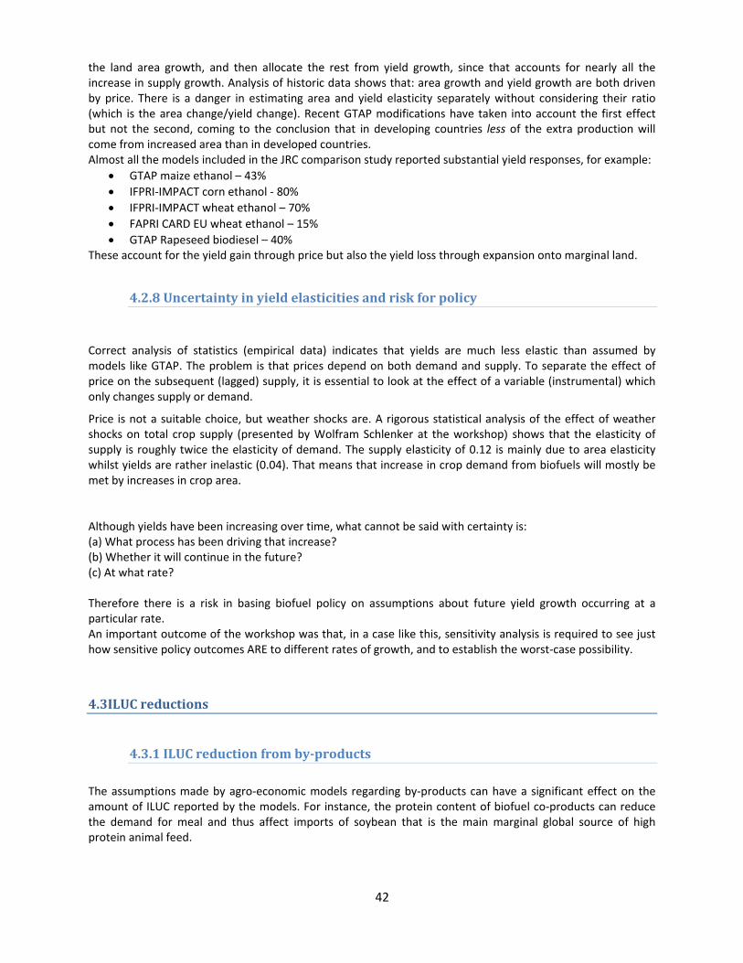
42  

the  land  area  growth,  and  then  allocate  the  rest  from  yield  growth,  since  that  accounts  for  nearly  all  the increase in supply growth. Analysis of historic data shows that: area growth and yield growth are both driven by price. There  is a danger  in estimating area and yield elasticity  separately without  considering  their  ratio (which  is  the area change/yield change). Recent GTAP modifications have  taken  into account  the  first effect but not  the  second, coming  to  the conclusion  that  in developing countries  less of  the extra production will come from increased area than in developed countries. Almost all the models included in the JRC comparison study reported substantial yield responses, for example: 

• GTAP maize ethanol – 43% • IFPRI‐IMPACT corn ethanol ‐ 80%  • IFPRI‐IMPACT wheat ethanol – 70% • FAPRI CARD EU wheat ethanol – 15% • GTAP Rapeseed biodiesel – 40% 

These account for the yield gain through price but also the yield loss through expansion onto marginal land.  

4.2.8Uncertaintyinyieldelasticitiesandriskforpolicy  Correct  analysis  of  statistics  (empirical  data)  indicates  that  yields  are much  less  elastic  than  assumed  by models  like GTAP. The problem  is that prices depend on both demand and supply. To separate the effect of price on the subsequent (lagged) supply, it is essential to look at the effect of a variable (instrumental) which only changes supply or demand.  

Price  is not a suitable choice, but weather shocks are. A rigorous statistical analysis of the effect of weather shocks on  total crop supply  (presented by Wolfram Schlenker at  the workshop) shows  that  the elasticity of supply  is roughly twice the elasticity of demand. The supply elasticity of 0.12  is mainly due to area elasticity whilst yields are rather inelastic (0.04). That means that increase in crop demand from biofuels will mostly be met by increases in crop area.   Although yields have been increasing over time, what cannot be said with certainty is:  (a) What process has been driving that increase? (b) Whether it will continue in the future? (c) At what rate?    Therefore  there  is  a  risk  in  basing  biofuel  policy  on  assumptions  about  future  yield  growth  occurring  at  a particular rate.  An important outcome of the workshop was that, in a case like this, sensitivity analysis is required to see just how sensitive policy outcomes ARE to different rates of growth, and to establish the worst‐case possibility. 

4.3ILUCreductions 

4.3.1ILUCreductionfromby‐products The assumptions made by agro‐economic models regarding by‐products can have a significant effect on  the amount of  ILUC reported by the models. For  instance, the protein content of biofuel co‐products can reduce the  demand  for meal  and  thus  affect  imports  of  soybean  that  is  the main marginal  global  source  of  high protein animal feed.  

43  

It  is  essential  that  the models  differentiate  between  fodder  energy  and  protein  feed  as  farmers make  a balanced  feed plan based on  the appropriate amount given  to  the animals. The marginal  source of  fodder energy  (mainly  grain  crops)  is  very  different  from  the marginal  source  of  protein  (soy meal).  They  have different fertiliser application rates and yields and will have a different impact with regards to indirect land use change and environmental impacts. The  ratio of protein vs. energy varies  significantly  in different oil meals:  soy meal has high protein content, rapeseed medium content and palm kernel oil meal a very low content. The key differences between Soy meal and palm oil are presented below:  Soy meal is grown primarily for its meal: 

• Meal accounts for about 60% of the value of soy bean • The oil yield of soy is only about 10% of that of oil palm • Soy meal accounted for 83% of trade in high protein meals from 2006‐2009 • Soy meal accounted for 91% of growth in trade in high protein meals from 1999 to 2009 

 Palm oil is grown nearly entirely for its oil and is the marginal global source of vegetable oil 

• Oil accounts for about 98% of the value from oil palm • Palm accounted for 80% of growth in trade in high protein oils from 1999 to 2009 

 It was  demonstrated  that  an  LCA  approach  can  capture  these  significant  differences  between  fodder  and protein  sources29.  For  example,  if  more  rapeseed  oil  is  required  to  meet  biodiesel  demand,  then  more rapeseed meal will be produced, and thus more protein and more food energy will be available. The protein from the rapeseed meal displaces some soy meal (co‐produced with soybean oil) so less oil will be produced. This reduction in oil  is compensated by marginal vegetable oils (e.g. palm oil). The LCA calculation for solving this  considers  the  amount  of  rapeseed  oil  required,  and  then  accounts  for  the  co‐products,  the marginal source of oil (palm oil), the marginal source of protein (soy meal) and barley which  is the marginal source of feed  energy.  In  a  LCA  approach,  a  tonne  of  rapeseed  oil  causes  increased  production  of  palm  oil  and displacement of both soy meal and a small amount of barley.   If  equilibrium models  aggregate  all  of  the  oilseeds  in  a  region,  it  can  be  argued  that  the model  cannot differentiate between the effects of marginal meal and marginal oil demands.  It  is also  important that  in the models  that do disaggregate oil  seeds,  soybean  should be modelled as  the marginal  source of high protein meal, thus allowing for the reduced growth of soy bean production due to substitution of soy meal by biofuel by‐products.  Substitution  ratios  for  EU  biofuel  by‐products  based  on  balancing  protein  and  energy requirements in compound animal feed are shown in Table 1.  

 Table 1: Co‐product substitution ratios [presented by W. Lywood ‐ ENSUS] 

 

                                                            29Schmidt J H, Christensen P and Christensen T S (2009). Assessing the land use implications of biodiesel use from an 

LCA perspective. Journal of Land Use Science Vol. 4, No. 1–2, March 2009, pp 35–52  

Substitution Ratios for EU Biofuel co-products

Co-productSubstution for

soy mealSubstution for

cereal

CE Delft 2008Wheat DDGS 0.50 0.66Maize DDGS 0.45 0.69

Lywood et al 2009Wheat DDGS 0.59 0.39Maize DDGS 0.40 0.49Rape meal 0.61 0.15

ADAS 2010Current scenario Wheat DDGS 0.33Future high usage scenario Wheat DDGS 0.60

t / t of co-product

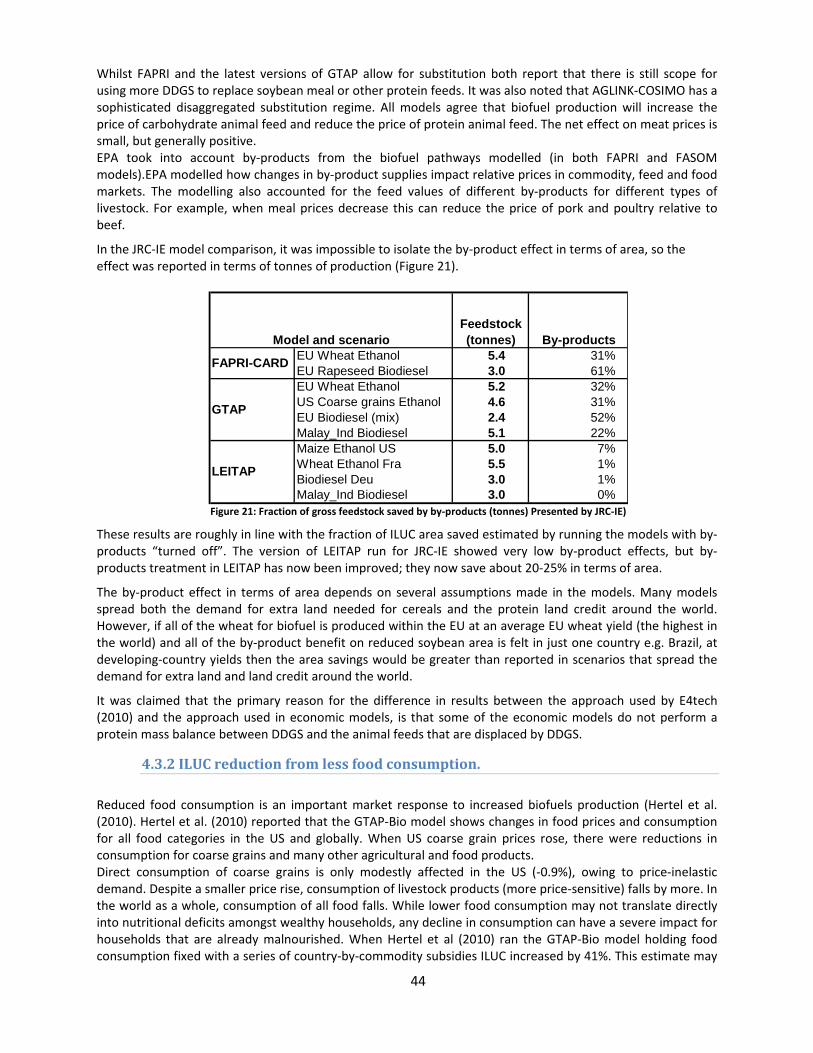
44  

Whilst FAPRI and  the  latest versions of GTAP allow  for  substitution both  report  that  there  is  still  scope  for using more DDGS to replace soybean meal or other protein feeds. It was also noted that AGLINK‐COSIMO has a sophisticated disaggregated  substitution  regime. All models  agree  that biofuel production will  increase  the price of carbohydrate animal feed and reduce the price of protein animal feed. The net effect on meat prices is small, but generally positive. EPA  took  into  account  by‐products  from  the  biofuel  pathways  modelled  (in  both  FAPRI  and  FASOM models).EPA modelled how changes in by‐product supplies impact relative prices in commodity, feed and food markets.  The modelling  also  accounted  for  the  feed  values  of  different  by‐products  for  different  types  of livestock. For example, when meal prices decrease  this can  reduce  the price of pork and poultry  relative  to beef.  

In the JRC‐IE model comparison, it was impossible to isolate the by‐product effect in terms of area, so the effect was reported in terms of tonnes of production (Figure 21).  

 Figure 21: Fraction of gross feedstock saved by by‐products (tonnes) Presented by JRC‐IE) 

These results are roughly in line with the fraction of ILUC area saved estimated by running the models with by‐products  “turned  off”.  The  version  of  LEITAP  run  for  JRC‐IE  showed  very  low  by‐product  effects,  but  by‐products treatment in LEITAP has now been improved; they now save about 20‐25% in terms of area.  

The by‐product effect  in  terms of area depends on several assumptions made  in  the models. Many models spread  both  the  demand  for  extra  land  needed  for  cereals  and  the  protein  land  credit  around  the world. However, if all of the wheat for biofuel is produced within the EU at an average EU wheat yield (the highest in the world) and all of the by‐product benefit on reduced soybean area is felt in just one country e.g. Brazil, at developing‐country yields then the area savings would be greater than reported  in scenarios that spread the demand for extra land and land credit around the world. 

It was  claimed  that  the primary  reason  for  the difference  in  results between  the approach used by E4tech (2010) and  the approach used  in economic models,  is  that some of  the economic models do not perform a protein mass balance between DDGS and the animal feeds that are displaced by DDGS.  

4.3.2ILUCreductionfromlessfoodconsumption. Reduced  food consumption  is an  important market  response  to  increased biofuels production  (Hertel et al. (2010). Hertel et al. (2010) reported that the GTAP‐Bio model shows changes in food prices and consumption for  all  food  categories  in  the US  and  globally. When US  coarse  grain prices  rose,  there were  reductions  in consumption for coarse grains and many other agricultural and food products.  Direct  consumption  of  coarse  grains  is  only modestly  affected  in  the  US  (‐0.9%),  owing  to  price‐inelastic demand. Despite a smaller price rise, consumption of livestock products (more price‐sensitive) falls by more. In the world as a whole, consumption of all food falls. While lower food consumption may not translate directly into nutritional deficits amongst wealthy households, any decline in consumption can have a severe impact for households  that are already malnourished. When Hertel et al  (2010)  ran  the GTAP‐Bio model holding  food consumption fixed with a series of country‐by‐commodity subsidies ILUC increased by 41%. This estimate may 

 

EU Wheat Ethanol 5.4 31%EU Rapeseed Biodiesel 3.0 61%EU Wheat Ethanol 5.2 32%US Coarse grains Ethanol 4.6 31%EU Biodiesel (mix) 2.4 52%Malay_Ind Biodiesel 5.1 22%Maize Ethanol US 5.0 7%Wheat Ethanol Fra 5.5 1%Biodiesel Deu 3.0 1%Malay_Ind Biodiesel 3.0 0%

By-productsModel and scenarioFeedstock (tonnes)

FAPRI-CARD

GTAP

LEITAP

45  

be thought of as a “food‐neutral” ILUC value or alternatively, as an ILUC value that translates food effects into units of GHG emissions. The  Californian  Air  Resources  Board  (ARB)  and  Hertel  et  al  (2010)  report  that  the  majority  of  models considered for the calculation of the Low Carbon Fuel Standard (LCFS) predict reductions in food (and/or feed and  fibre)  consumption,  representing part of  the process by which  land use  change  for biofuel production increase is not a hectare‐for‐hectare displacement of existing area (ARB, 2010). Keeping food consumption constant  in a model does not fully  illustrate the effects of how LUC with reduced food consumption because many other  factors change  in  the model as well.  JRC  (2010b) calculated  the net reduction in food and feed consumption reported by the several models using mass balance: 

Where: Net increase in world total crop production in tonnes (reported by model) equals Gross feedstock requirements for biofuels minus Tonnes of crops replaced by by‐products Minus  Reduction in food and feed consumption 

 JRC (2010b) showed that most of the models included in the comparison indicate a reduction in crops used for food and feed due to biofuels production. The percentage of food consumption reduction (after accounting for by‐products) was highest for ethanol scenarios, and was generally highest  in the models which reported the least ILUC (See Table 2) 

 Table 2: Food consumption reduction in JRC model comparison results (after by‐products have been accounted for). 

Arguably, this effect should not be included  in the calculation of ILUC emissions. If the effect is removed, the ILUC emissions  from all models  in  the  JRC modelling comparison would appear  to outweigh  the direct GHG savings  for  all  the biofuels with  the possible exception of  sugar‐cane ethanol  (which  is not  included  in  the calculations shown below).  In Table 3  the C content of  the  reduced  food consumption  in  total  (not  just  for individual  crops)  is  used  to  calculate  the  CO2  emissions  credit  from  the  food  consumption  reduction. Production emissions were calculated using JRC Well‐to‐Wheel study v3 values.  

 

Model and Type of Ethanol

Food Consumption Reduction (exclusive of by‐products)

GTAP US Maize 52%IMPACT US Maize 36%IMPACT EU Wheat 47%FAPRI CARD EU Wheat 34%GTAP EU Wheat 46%

Model and Type of Ethanol

Food Consumption Reduction (exclusive of by‐products)

GTAP US Maize 52%IMPACT US Maize 36%IMPACT EU Wheat 47%FAPRI CARD EU Wheat 34%GTAP EU Wheat 46%

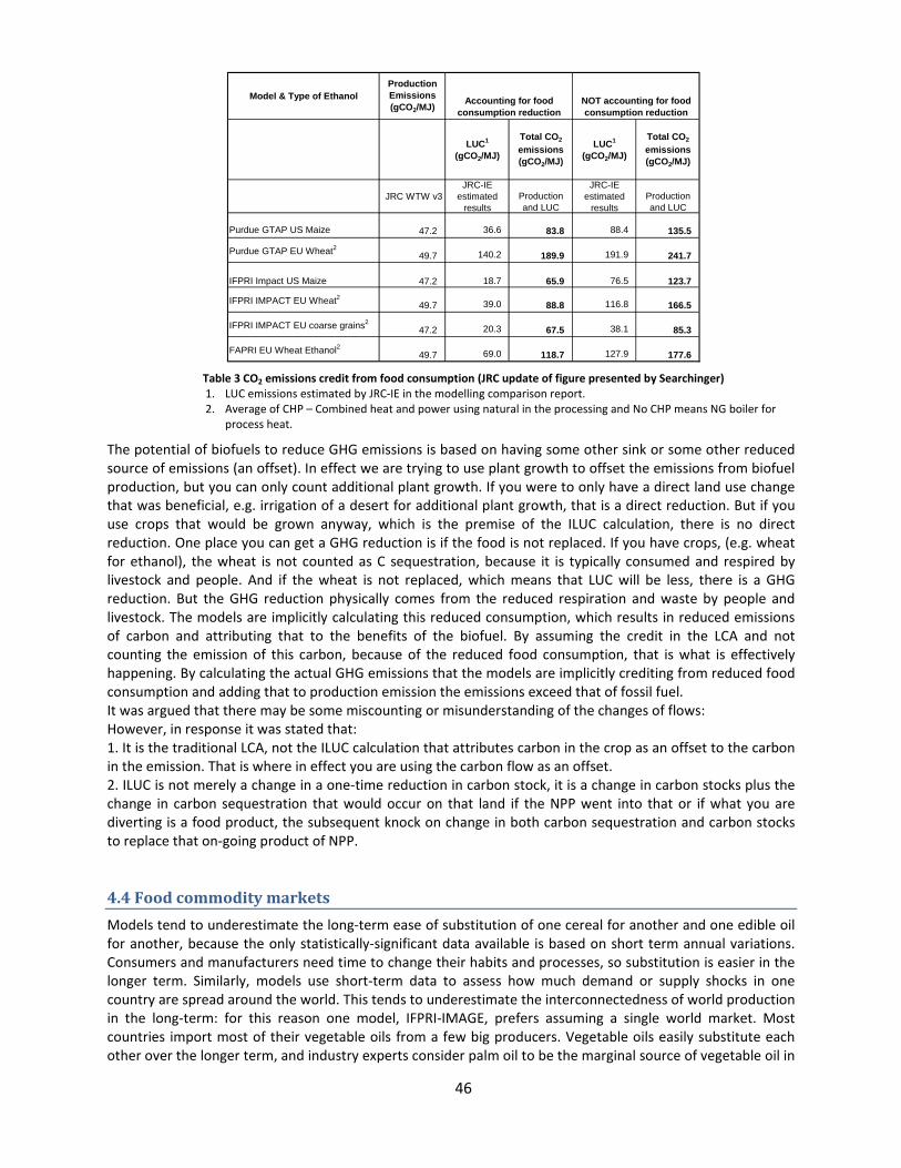
46  

 Table 3 CO2 emissions credit from food consumption (JRC update of figure presented by Searchinger) 1. LUC emissions estimated by JRC‐IE in the modelling comparison report. 2. Average of CHP – Combined heat and power using natural in the processing and No CHP means NG boiler for 

process heat. 

The potential of biofuels to reduce GHG emissions is based on having some other sink or some other reduced source of emissions (an offset). In effect we are trying to use plant growth to offset the emissions from biofuel production, but you can only count additional plant growth. If you were to only have a direct land use change that was beneficial, e.g. irrigation of a desert for additional plant growth, that is a direct reduction. But if you use  crops  that would  be  grown  anyway, which  is  the  premise  of  the  ILUC  calculation,  there  is  no  direct reduction. One place you can get a GHG reduction is if the food is not replaced. If you have crops, (e.g. wheat for ethanol),  the wheat  is not counted as C sequestration, because  it  is  typically consumed and  respired by livestock  and people. And  if  the wheat  is not  replaced, which means  that  LUC will be  less,  there  is  a GHG reduction. But  the GHG  reduction physically  comes  from  the  reduced  respiration and waste by people and livestock. The models are  implicitly calculating this reduced consumption, which results  in reduced emissions of  carbon  and  attributing  that  to  the  benefits  of  the  biofuel.  By  assuming  the  credit  in  the  LCA  and  not counting  the emission of  this  carbon, because of  the  reduced  food  consumption,  that  is what  is effectively happening. By calculating the actual GHG emissions that the models are implicitly crediting from reduced food consumption and adding that to production emission the emissions exceed that of fossil fuel.  It was argued that there may be some miscounting or misunderstanding of the changes of flows: However, in response it was stated that: 1. It is the traditional LCA, not the ILUC calculation that attributes carbon in the crop as an offset to the carbon in the emission. That is where in effect you are using the carbon flow as an offset. 2. ILUC is not merely a change in a one‐time reduction in carbon stock, it is a change in carbon stocks plus the change  in carbon sequestration  that would occur on  that  land  if  the NPP went  into  that or  if what you are diverting  is a food product, the subsequent knock on change  in both carbon sequestration and carbon stocks to replace that on‐going product of NPP. 

 

4.4FoodcommoditymarketsModels tend to underestimate the long‐term ease of substitution of one cereal for another and one edible oil for another, because the only statistically‐significant data available  is based on short term annual variations. Consumers and manufacturers need time to change their habits and processes, so substitution is easier in the longer  term.  Similarly, models  use  short‐term  data  to  assess  how much  demand  or  supply  shocks  in  one country are spread around the world. This tends to underestimate the interconnectedness of world production in  the  long‐term:  for  this  reason  one model,  IFPRI‐IMAGE,  prefers  assuming  a  single world market. Most countries  import most of their vegetable oils  from a few big producers. Vegetable oils easily substitute each other over the longer term, and industry experts consider palm oil to be the marginal source of vegetable oil in 

Model & Type of EthanolProduction Emissions (gCO2/MJ)

LUC1

(gCO2/MJ)

Total CO2

emissions (gCO2/MJ)

LUC1

(gCO2/MJ)

Total CO2

emissions (gCO2/MJ)

JRC WTW v3JRC-IE

estimated results

Production and LUC

JRC-IE estimated

resultsProduction and LUC

Purdue GTAP US Maize 47.2 36.6 83.8 88.4 135.5

Purdue GTAP EU Wheat2 49.7 140.2 189.9 191.9 241.7

IFPRI Impact US Maize 47.2 18.7 65.9 76.5 123.7

IFPRI IMPACT EU Wheat2 49.7 39.0 88.8 116.8 166.5

IFPRI IMPACT EU coarse grains247.2 20.3 67.5 38.1 85.3

FAPRI EU Wheat Ethanol2 49.7 69.0 118.7 127.9 177.6

Accounting for food consumption reduction

NOT accounting for food consumption reduction

47  

the world, as  it has a production‐cost advantage and hardly competes with other crops. That means use of vegetable oils or animal  fats  for biodiesel will, on a decade‐timescale,  largely be met by  increased palm oil production. Cereals clearly can also easily more easily substitute each other in the long term. In general, crop production has shifted increasingly to land‐rich countries in S. America. An exception to this trend is EU, India and  China  which,  historically,  kept  cereals  production  mostly  just  ahead  of  demand  by  adjustments  to domestic  agriculture  policies  and  trade  barriers.  However,  free‐trade  agreements  (which  are  taken  into account in economic models) limit the EU’s power to do this in the future. Therefore, in the future, increased EU  cereals  demand  is  likely  to  be met  largely  by  imports  or  reduced  exports,  rather  than  changes  in  EU production. One of  the main  reasons  for building  the economic models was  to see how  these conditions of trade will affect future markets.   Substitution of oilseeds and animal fats  In the context of estimating critical issues in the ILUC emissions, it is important to understand what happens if there will be more demand for rapeseed oil or animal fats, and what they could be replaced with. The National Renewable Energy Action Plans (NREAPs) for EU member states show that approximately 74%30 of the biofuel target in 2020 will be biodiesel, which implies that oil and fats are an issue. The NREAPs show that the EU will need about 22 Mt of natural oils and fats by 2020, to meet the 10% target. EU production is unlikely to keep up with demand, and there will be an  increasing need to import, which will have a substantial  impact on the global balance of oils and fats price relationships. These oils are now closely trading in line with the petrol/oil prices, and this is not driven by supply, demand, yield increase, area or farmers knowledge, but by the market speculation. 

The world’s  supply  in  oil  and  fats  is  approximately  165 Mt,  and  the  average  increase  over  the  past  years (inclusive of any European biofuel increase) is 5‐7 Mt. 75% of those oils and fats are used in food nutrition, 6% in animal feed, 10% in olio chemicals, and 9% for biofuels (see presentation from Klaus Nottinger, APAG) . Half of the world’s supply of oil and  fats comes  from palm oil and soy, so the critical  issue of  ILUC will continue. Area  increase  and  yield  improvements  in  palm  oil  have  been  significant  though  the  area  effect  has  been stronger  than  the  yield effect.  In  contrast  to  the  increase  in palm oil production,  the  increase  in  rapeseed production  has  been much  less  significant.  Indonesia  is  overtaking Malaysia  in  palm  oil  production mainly because Malaysian production growth on available  land has been  limited because of ecological  reasons and other impacts.  

Palm oil is a direct substitution for tallow (a co‐product from meat production). Most of the palm oil produced is exported and accounts for 60% of all the World’s exported oils and fats, whereas soy and rapeseed exports are declining. For biofuel legislation, as well as food demand (at least for India and China) palm oil is helping to fulfil those demands. European consumption of rapeseed oil has been driven by biofuels (67%  in 2010), with the remainder for food and other uses. The  limitations of rapeseed oil production  in the EU are already at a certain limit and any additional demand will have to come from palm oil.  

In many applications the only substitution  for palm oil  is tallow. The variety of applications of tallow means that the negative ILUC emission issue will catch consumer attention, because it will impact the daily lives of the people worldwide. It is often assumed that animal fat is waste or a residue and that using it as a biofuel would allow the legislation to conclude that it should have significant GHG savings. However, this product is actually in direct conflict with a vegetable oil, which will  increase GHG emissions. Rather  than a credit  it will have a debit  of  at  least  the  palm  oil  number  plus  the  rendering  process.  In  conclusion  these  animal  by‐products cannot be considered waste, as they have a ready market.  

     

                                                            30 NREAPS for 26 countries, excluding Hungary indicate a 74% share for biodiesel in total biofuel consumption – JRC‐IE 

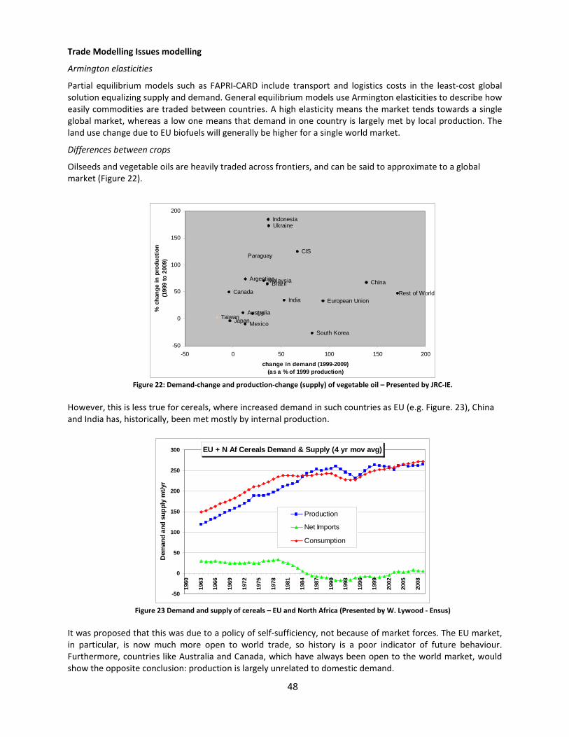
48  

Trade Modelling Issues modelling 

Armington elasticities 

Partial equilibrium models  such as  FAPRI‐CARD  include  transport and  logistics  costs  in  the  least‐cost  global solution equalizing supply and demand. General equilibrium models use Armington elasticities to describe how easily commodities are traded between countries. A high elasticity means the market tends towards a single global market, whereas a  low one means that demand  in one country  is  largely met by  local production. The land use change due to EU biofuels will generally be higher for a single world market.  

Differences between crops 

Oilseeds and vegetable oils are heavily traded across frontiers, and can be said to approximate to a global market (Figure 22). 

 

 Figure 22: Demand‐change and production‐change (supply) of vegetable oil – Presented by JRC‐IE. 

 However, this is less true for cereals, where increased demand in such countries as EU (e.g. Figure. 23), China and India has, historically, been met mostly by internal production.  

 Figure 23 Demand and supply of cereals – EU and North Africa (Presented by W. Lywood ‐ Ensus) 

 It was proposed that this was due to a policy of self‐sufficiency, not because of market forces. The EU market, in  particular,  is  now much more  open  to world  trade,  so  history  is  a  poor  indicator  of  future  behaviour. Furthermore, countries  like Australia and Canada, which have always been open to the world market, would show the opposite conclusion: production is largely unrelated to domestic demand.  

Argentina

Australia

Canada China

CIS

European Union India

Indonesia

Malaysia

Mexico

Rest of World

South Korea

Taiwan

Ukraine

Us

Brazil

Japan

Paraguay

-50

0

50

100

150

200

-50 0 50 100 150 200

change in demand (1999-2009) (as a % of 1999 production)

% c

hang

e in

pro

duct

ion

(199

9 to

200

9)

EU + N Af Cereals Demand & Supply (4 yr mov avg)

-50

0

50

100

150

200

250

300

1960

1963

1966

1969

1972

1975

1978

1981

1984

1987

1990

1993

1996

1999

2002

2005

2008

Dem

and

and

supp

ly m

t/yr

Production

Net Imports

Consumption

49  

 Should Armington Elasticities be differentiated between crops? Because of these differences, it was suggested that Armington elasticities should be made crop‐dependent and tuned to match historical trade data for each crop. But cereals and oilseeds are grown on the same land: thus, for example, an increase in demand for cereals in EU would be met partly by more oilseed imports. Therefore there is an argument for a single value which refers to land substitution as a whole.  Are Armington Elasticities chosen appropriately? There are large differences between the Armington elasticities for different models: GTAP uses a value of 2.6, whereas  IFPRI‐MIRAGE  uses  10, which  seems  arbitrary. However,  this  is  because  the GTAP  value  is  for  an aggregate  of  cereals, whereas  the  IFPRI  value  is  applied  to  individual  cereals.    As  individual  cereals  easily substitute each other, the world market can easily adjust to supply more of a particular cereal to one country. Armington elasticities are chosen to be consistent with observed price transmissions between markets: a high value  is needed  to explain why  the price of a commodity  in one country  is heavily  influenced by  the world price.  Short‐term vs. long‐term data It was proposed that modelers systematically underestimate both long‐term Armington elasticities, and long‐term elasticities of substitution between crops.   That  is because the only data available  is short‐term annual data, whereas the models are applied to changes over a decade. It takes time for consumers and processors to adapt  to  a  different  type  of  cereal  or  vegetable  oil  from  a  new  source‐country.    Therefore  short‐term elasticities are too  low  in  the context of a  long‐term model. This means that models  tend  to underestimate land  use  change  in  exporting  countries,  and  to  overestimate  the  differences  in  land  use  change  between different feedstocks.  

  

 

Tudinat(

Inept(m

Afoetw

T

 

 

5. SensTo  estimate understand  tdemand  can ncreased proand how muche changes iblue bars). 

 ntensificatioetc.) and usiproperly accohrough intenland  use  chmatch policy 

 Another impoor  fuels  (whethanol or Brwo very diffe

 There are thr

1. The dthesegive d

2. The  rprovi

3. A gov 

sitivityandthe  effects

that  there  abe met  eithoduction. In ch from intein productio

Figure 2

n itself bringng  LCA  coefount for C ensification, uange,  reducchoices to d

ortant aspechich  reflect  trazilian sugaerent concep

ree distinct vdifferent moe estimates tdifferent valreal “physicaided by the mvernment th

duncertais  of  incremeare  additionaher  through the latter cansification. An will come 

24 Decompositi

gs additionalfficients  thatmissions.  It unless the abction  in  fooddesired outco

ct that needstheir  climater cane ethanpts. 

variables for odels  (such athe GW effeues for eachal” GWI  is nmodels. en decides o

intiesinmental  demanal  “costs”  tha  reduction

ase it is neceAs shown in from LUC (g

ion between yi

 “costs” (mot are  compuis not corre

bove additiond  consumptiomes better 

s to be consie  impact)  thnol) do not 

a single fuelas  IFPRI) maect of a MJ‐f fuel type. ot known an

on an 'operat

50 

modellingsnd  for  biofuhat  have  to n  in  (food)  cessary to knoFigure 24 (frreen bars), a

eld and land ex

ore irrigationuted  for  just ct  in principnal costs are on  and  intethan compu

dered is thaat  are used necessarily r

: ake an estimfor‐MJ subst

nd  is a  rand

tional’ GWI o

studiesuels  with  ebe  conside

consumptionow how mucrom IFPRI anand less prod

xtension [prese

n, more enerone  techno

ple to assumproperly acc

ensification) ting only lan

t “Operationin policy  (fo

reflect the fu

mate of  the “itution of on

om variable

of fuel to pub

conomic  moered:  for  insn, with  low ch of the incnalysis), for tduction will 

ented by D. Lab

rgy consumpology  (“non‐e that LUC ecounted for.together w

nd use effect

nal” Global Wor example uels’ actual c

“physical” GWne fuel for a

, but eviden

blish (e.g. in 

odels,  it  is tance,  increLUC, or  canrease will cohe crops selcome from i

borde – IFPRI] 

tion, more mintensificatioemissions ar  Estimating ill  reduce  erts. 

Warming InteCARB  valueclimate effec

WI of a biofnother.   Diff

nce about  th

LCFS implem

important  teased  biofue  be met witome from LUected most ointensificatio

 

mechanizatioon”) does nore “mitigatedall the effecrrors  and w

ensities (GWs  for US  corcts. These ar

fuel. A pair oferent mode

he  real GWI 

mentation) 

to els th UC of on 

on ot d” ts 

will 

WI) rn re 

of els 

is 

Tt1baim2aupTrv

of

Vv

T(dfta 

 

The optimal votal social va1. The uncerbetween opeanalysis that mplied by a s2. The result a more compunregulated policy, and vaThe “operatioeflect  their value for eac

‐ How bigonly  parameunctional rel

‐ What is ‐ How can

Various studivarying param

1 Elasticit2 Elasticit3 Elasticit4 Elasticit5 Share o6 Elasticit7 Margin

They used thdomestic prorom biodieshe  Figure  25approximate 

Figure 25: 

value for thisalue of all kintainty assocerational andin these cirstandard cenof implemenplicated respmarkets, noarious kinds onal” numbeintrinsic unch fuel. The fug  is  the unceter  uncertalationships athe form of n we deal wi

ies are on‐gometers: 

ty on the usety of substituty between lty of manageof expansion ty of cattle inal yields 

ree differentoduction), oel. Prelimina5, with  valurange 40 – 9

results of Mon

s last variablnds–is not neiated with  td  real physiccumstances,ntral estimatnting a policponse  involvon‐fuel‐relateof rent‐seekers depend ocertainties, wundamental ertainty  in ainty,  but  suamong paramthis uncertaith it in legisl

oing: IFPRI fo

e of inputs ution of landlow substituted land expain primary fntensificatio

t scenarios fone on ethanary  results, oes  for  ethan90 gCO2eq/MJ

nte Carlo analys

e–the value ecessarily thhe physical cal GWI) ma, the optimator of the uncy with a giveing the related  regulatoring. on the modewhich  then cquestions foa given estimubstantial mmeters, and eainty? lation and po

or example 

d among croptable cropsansion orest n 

or a 7% manol with tradeobtained usinol  in  the  raJ. 

sis on Land Use

51 

that produce most likelyGWI  is asymy also be asal action  for certain randen operationtive prices ofry changes o

els and assumcause probleor the policy mate and acodel  uncerteven which p

olicy implem

is carrying o

ps  

ndate of biofue liberalizatiing a uniformange  of  abo

 e emissions fro

es either they value of a fmmetric, andsymmetric.   a decision mom variablenal GWI is nof the fuels, soutside  the  j

mptions usedems  in decisprocess are ross all estimainty,  i.e.  laparameters t

mentation? 

out Monte C

uels for tranon and one m distributioout  20  to  55

om IFPRI – MIRA

e least globafuel’s physicad  the cost ofIt  is a convemaker may b. ot MJ‐for‐MJshifting of fuurisdiction  i

d to estimateion analysis then: mates?  Impoack  of  knowto incorporat

arlo simulat

sport in the where all inon probabilit5  gCO2eq/MJ,

AGE model [Pre

l warming, oal GWI, for twf being wronentional  resube different 

J substitutionuels among rmplementin

e the real GWto define a

ortantly,  thiswledge  aboute into the m

ions, with th

EU: one bascremental bty  function, ,  and  for  bio

 

esented by D. L

or the greatewo reasons: ng  (differencult of decisiofrom the on

n of fuels, buregulated ang  the origin

WI values ann appropriat

s  includes nout  the  corremodel. 

he following 

ed on ethaniofuels comeare  shown odiesel  in  th

Laborde – IFPR

st  ce on ne 

ut nd al 

nd te 

ot ct 

7 

ol es in he 

RI] 

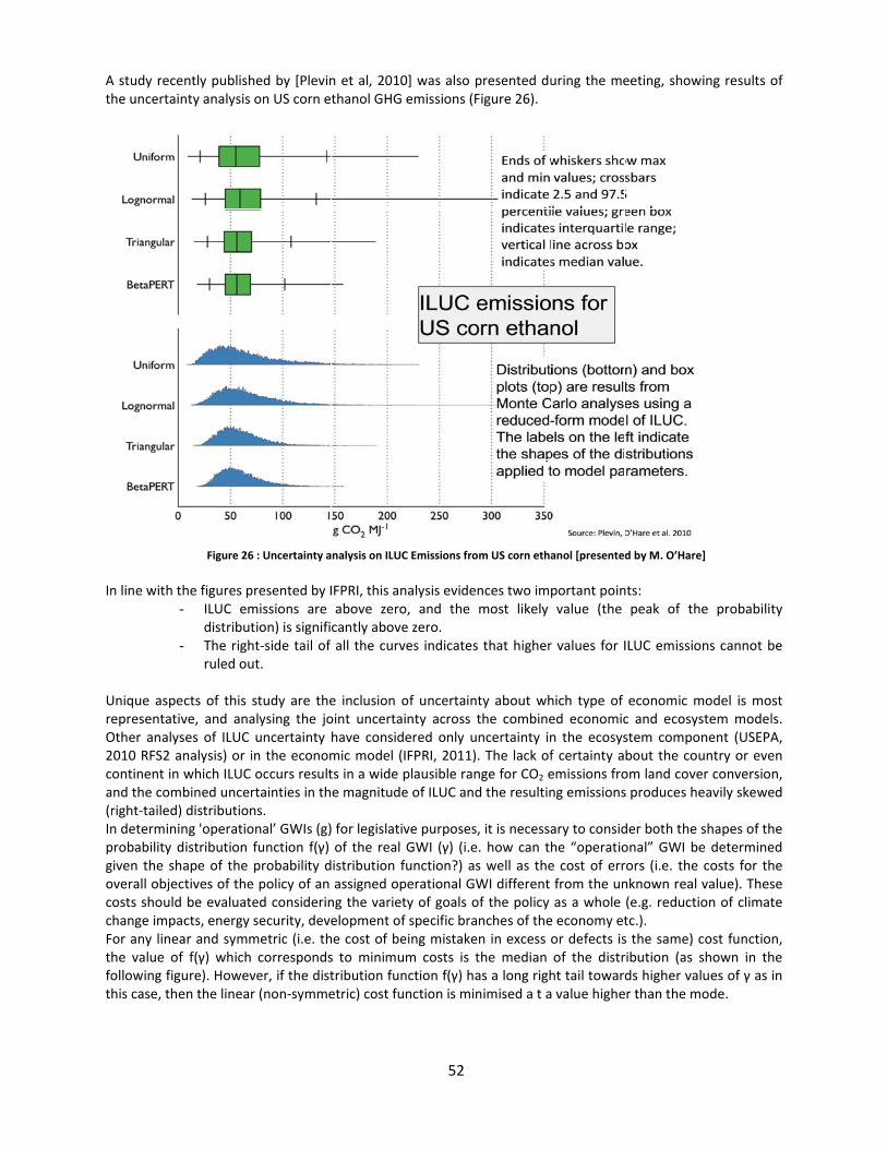
At

In

UrO2ca(InpgoccFtfot 

 

A study recehe uncertain

 n line with th

-

-

 Unique aspecepresentativOther analys2010 RFS2 ancontinent in wand the combright‐tailed) n determininprobability dgiven  the shaoverall objeccosts should change impacFor any  lineahe  value  of ollowing figuhis case, the

  

ntly publishenty analysis o

Figure 26 :

he figures prILUC  emdistributiThe rightruled out

cts of  this  stve,  and  anales of  ILUC unalysis) or  inwhich ILUC obined uncertdistributionsng 'operationistribution  fape of  the ptives of the be evaluatects, energy sar and symmf(γ) which 

ure). Howeveen the linear 

ed by [Plevinon US corn e

: Uncertainty a

resented by Iissions  are ion) is signifit‐side tail of t.   

tudy are  thelysing  the  jouncertainty n the economoccurs resulttainties in ths. nal’ GWIs (g)unction  f(γ) probability dpolicy of an ed considerinsecurity, devemetric (i.e. thcorrespondser, if the dist(non‐symme

n et al, 2010thanol GHG 

nalysis on ILUC

IFPRI, this anabove  zerocantly aboveall the curv

e  inclusion ooint  uncertaihave  considmic model  (Its in a wide pe magnitude

 for legislativof  the  real istribution  fassigned opng the varietelopment ofhe cost of bes  to minimutribution funetric) cost fu

52 

0] was also pemissions (F

                        

C Emissions fro

nalysis evideno,  and  the e zero. ves  indicates

of uncertaintinty  across  tered only uIFPRI, 2011).plausible rane of ILUC and

ve purposes,GWI  (γ)  (i.efunction?) asperational GWty of goals of specific braeing mistakem  costs  is  tnction f(γ) hanction is min

presented duFigure 26).  

m US corn etha

nces two impmost  likely 

 that higher

ty about whthe  combinencertainty  in. The  lack ofnge for CO2 ed the resultin

, it is necessa. how can  ths well as  theWI different of the policy nches of then  in excess othe median as a long righnimised a t a

uring the me

anol [presente

portant poinvalue  (the 

r values  for  I

hich  type of ed  economicn  the ecosysf certainty aemissions frong emissions

ary to considhe “operatioe cost of errfrom the unas a whole 

e economy etor defects  isof  the  distrht tail towar value highe

eeting, show

d by M. O’Hare

nts: peak  of  th

ILUC emissio

economic mc  and  ecosystem  compobout the coom land coves produces h

der both the onal” GWI brors  (i.e.  thenknown real (e.g. reductitc.). s the same) ribution  (as ds higher vaer than the m

wing results o

e] 

he  probabilit

ons cannot b

model  is mostem modelonent  (USEPAuntry or eveer conversioeavily skewe

shapes of the determine costs  for  thvalue). Thesion of climat

cost functioshown  in  thlues of γ as 

mode. 

of 

ty 

be 

st ls. A, en n, ed 

he ed he se te 

n, he in 

5

Aaptae

Ita 

 

                   

5.1ILUCan 

At present, ba 50% direct per tonne of he  costs  sigabatement  ceffective.  

 

Figure 27 A 

t  is  then  cleabatement, a

                 31 or aroun

ndcostofc

iofuels are gsaving againf carbon dioxgnificantly.  Inost  rises  to 

Abatement cost

ear  that  inveand it is there

                      nd $240 per t

carbonaba

generally connst an 86.4 gxide saved,  in  the  examp$1000. This

ts as a function

esting  in  carbefore worthw

 

                     onne of fuel f

atement�

nsidered to bgCO2e/MJ foignoring  iLUple  shown  ins  is of  intere

n of ILUC emiss

bon abatemwhile.  

for biodiesel53 

be more expeossil fuel comC  (based onn  Figure  27,est as often 

ions (presente

ent measure

ensive than fmparator the JRC 2008).  with  ILUC policy decis

d by C. Malins 

es  to mitiga

fossil fuels. Ee cost for caIncluding  ILemissions  oions are bas

– The ICCT) 

te  ILUC will 

E.g. for a biorbon abatemUC emissionf  35gCO2/Msed on what

bring  to  su

fuel achievinment  is $150ns would raisJ,  the  carbot  is most  co

bstantial  co

ng 031 se on st 

st 

5

WmApstAinareWm

ItfeWh(tObabgABcAo

 

5.2Mitigat

While  it is  immitigate thesAt the global‐pressure fromupply chain erm solutionAt the produndirect effecadvantage  thesidues,  algeffectively exWhen ILUC emost of the f

 

Figure 

t is thus veryeedstock witWhat  is caushave to be avN.B. This canhan indirect One  way  thibiodiversity  aabandoned labe  economicgrassland to pAnother way Brazil with  thcattle densityA detailed anout.  

                 32  A small

tingtheris

mportant to kse indirect ef‐level prevenm the agricuefficiencies ns.  cer  level, prcts. One optihat  can  inceae  etc.),  buxcludes manymissions areeedstock wo

 28 GHG emiss

y important thout the indsing  ILUC  is  tvoided, biofun still result land use chais  could  be and  carbon and). For exacally  better palm oil mayto avoid dishe productioy and avoidinnalysis of the

                       amount of ba

skofunwa

know the sizffects. nting unwanultural sectorand/or a red

roduction of ion to do thientivize  the t  it  does  noy feedstockse added to thould fail to m

ions from seve

also to impldirect effectsthe displaceuels should gin direct landange).  achieved  isstocks,  alsoample expanthan  expany be positiveplacement ison of sugar cng displaceme impact of i

                     agasse is used

antedindir

ze of the ILU

ted “direct” r on  land exduction in co

biofuel feedis could be tuse  of  feedot  provide  a.  he typical REmeet the 50%

eral feedstocks 

ement addits. ment of  foogrow withoutd use change

s  by  expando  avoiding  ansion of palmsion  onto  p.  s to integratcane. The cament to new mplementat

d in co‐genera54 

recteffects

C effect it is

LUC in othepansion as aonsumption.

dstocks shouto add a feedstocks with any  incentive

D values for % threshold fo

compared to f

tional measu

od productiot any displace but that pr

ding  productany  loss  in  cm oil on Impepeatland.  In 

e the producattle could bpasture landtion of these

ation but this s

s

s equally  imp

r sectors wila whole can. Both of the

uld be expandstock specia  low  ILUC es  for  how 

direct GHG or GHG savin

ossil fuel comp

ures and sust

on  to biofuelement occurroblem may 

tion  on  unucarbon  sequerata grasslaaddition  th

ctivity of nonbe  fed with hd. e measures o

still leaves a la

portant to kn

l also prevenalso be redese measure

nded minimizfic ILUC factrisk  (e.g.  suthese  feeds

emissions (Fngs that will 

parator. [presen

tainable pro

ls. Thereforerring.  be more ide

used  or  unduestration  (end has greathe  C  effects 

n –bioenergyhydrolysed b

on biofuels c

arge amount 

now what ca

nt the indirecuced by  incres are compa

zing the riskor. This appugar‐cane,  litocks  are  cu

Figure 28) it icome into fo

nted by B. Deh

duction prac

e,  if  these  in

entifiable an

derutilised  lae.g.  from  afft potential aof  going  fr

y systems subagasse32,  th

osts has still

left for anima

an be done t

ct effects. Threasing yieldaratively long

k of unwanteroach has thignocellulosiultivated,  an

s evident thaorce in 2017

 ue – Ecofys] 

ctices to gro

ndirect effec

d controllab

and  with  loforestation  ond appears trom  Imperat

ch as cattle hus  increasin

l to be carrie

al feed 

to 

he ds, g‐

ed he c, nd 

at . 

w 

ts 

le 

w of to ta 

in ng 

ed 

ItpTfoTfov 

Mf

 

t was also uproduction syThe risk of ILUor example iThe figure beossil based vehicles (from

Figure 29:   

Moreover, thigure below 

 

 Figure 30 : 

nderlined duystems as shUC could alsoincentivizingelow shows tmobility  in  Sm PV or coge

Fossil fuels sub

he improvempresented b

GHG saving po

uring  the disown here too be minimiz the use of ethe results oSwitzerland.eneration) is 

bstitution acco

ment of vehicby EMPA (CH

otential in Swit

scussion  thao capture thezed through electric cars aof an analysis  It  is  evidenhigher than 

rding to differe

les efficiency). 

zerland (presen

55 

at better  lane full potentiother policyand improvins carried outnt  from  the the one of a

ent scenarios (p

y has the pot

nted by J. Rein

d cover dataal.  y actions andng vehicle eft by EMPA (Cfigure  that 

all biofuels (1

presented by J.

tential to sav

hard – EMPA)

a  is needed 

 supplementfficiency to rCH) on the pthe  substitu1st and 2nd ge

. Reinhard – EM

ve higher GH

to  investiga

tary measureeduce the deotential of sution  potenteneration).  

 MPA) 

HG than biofu

 

te alternativ

es to biofuelemand for oubstitution otial of  electr

uels, as from

ve 

ls, il. of ric 

m 

56  

6. PolicyrecommendationsonILUC 

The main objective of this section is to discuss and provide answers to the following policy‐relevant questions:   Based on the available science, can we conclude that the GHG impacts from ILUC of the EU biofuel/bioliquids policy are significant? Can  we  differentiate  the  impacts  between  different  feedstock  types,  the  geographical  location  of  the feedstocks (e.g. is there a difference in the GHG impact depending on where the biofuel feedstocks are grown) and what effect do different land management/mitigation practices have.  This section includes the discussion held by the invited experts on the main policy questions (shown in bold in the following paragraphs) put forward by the Commission. 

The views expressed in this report are those of the experts who participated to the workshop only, and do not represent the opinion of the Commission  Can we conclude that the GHG ILUC impacts of EU biofuel/bioliquids policy are significant? There was consensus that: None of the data (including uncertainties) indicate that ILUC is zero or not significant. Most of the studies indicate that biodiesel has a higher ILUC impact then ethanol, while the demand for diesel is higher than for gasoline in the EU.  Differences in models have been largely discussed, and it was agreed that ILUC estimations are lower in some models, mainly due to:  1. Lower rate of forest conversion 2.  Larger GHG benefits  from a  reduction  in  food  consumption:  it was agreed  that model estimates of  ILUC should not include a reduction of food consumption, or at least this shouldn’t be attributed an “ILUC benefit” to biofuels.  3. High Armington  elasticities: models which  assume high  values  for Armington  elasticities have  little  crop displacement outside the region of the increased demand and most apportion production to high yield areas  There  are  of  course  other  reasons  for  differences  between  models  (like  the  use  of  co‐products,  yield elasticities, marginal yields etc.), but all this has been exhaustively explained in the previous chapters.   Can we differentiate between different geographical locations?  Although  there  is  evidence  that  emissions  from  the  same  feedstock  (e.g.  soybean)  vary  according  to geographic location, it is quite difficult to differentiate because markets are globally connected and there are uncertainties on the  identification of the region where  ILUC occurs  (discrimination has also to be avoided  in policy).  A possibility to account for geographic differences could be to consider the productivity of  lands  in different geographic locations and using a “weighted factor” according to Net Primary production (NPP) of the land. For instance the weighting factor will be higher in Malaysia/Indonesia because the productivity in these regions is higher  than  for  example  in  the  EU  (i.e.  one  ha  in Malaysia will  have  double  the NPP  than  in  Europe,  and therefore one ha in one year in EU will have half the ILUC than in one ha in one year Malaysia/Indonesia, but it must be also considered that the biofuel produced from EU land will also be less).  Can we recommend Land management and Mitigation practices? Policy makers shall  implement additional mitigation criteria and  incentivize mitigation practices as the use of degraded land where food crops are not grown or intensification. Concerning  the use of degraded  land,  it was  stated  that  cost benefit analysis  and efficiency  considerations favour biomass crops such as eucalyptus to store CO2 over growing biofuel feedstocks.  Encouragement of good food policies/practices that for example incentivise intensification on pasture land will certainly bring to ILUC reductions. Models assuming a large pasture intensification effect versus extensification 

57  

have also  lower  ILUC effects. The  intensification of cattle production  in Brazil  (together with high yield and direct GHG saving from co‐generation) results in lower ILUC from sugar cane than from other feedstocks, and this management practice should be incentivized by appropriate policies. Increasing the yields could also mitigate ILUC effects, but the data shown by a number of studies seems to be more promising than the reality. Additional  incentives  for  mitigation  of  land  use  change  emissions  could  move  a  biofuel  above  the  RED threshold for GHG savings.   Should the GHG threshold be increased? The majority of experts agreed that increasing the GHG threshold, whilst bringing improvements to processes (e.g. methane capture in oil palm refineries), will not be effective for ILUC reduction. The opinion of the invited experts was  that a general  increase of  the  threshold will equally penalize all biofuels, without  “rewarding” those not  causing  ILUC  (or  causing  reduced  ILUC).  There  should  instead be  a distinction between different pathways, incentivizing the use of “low ILUC risk” biofuels.  Moreover, the increase of the GHG threshold will not benefit biodiversity or reduce competition with food etc. Other policy options  (e.g. additional  incentives  for biofuels with  low  ILUC  risk, obtained by use of degraded land or by specified mitigation practices, use of crop‐specific “ILUC factors”) would therefore be preferable in the opinion of the scientists.   Should we apply an “ILUC factor”? The  use  of  a  crop‐specific  factor which  attributes  a  quantity  of  greenhouse  gas  emissions  to  biofuels was generally  recommended, as  it  incentivizes directly  the production and use of  fuels with  low estimated  total Carbon  Impact. Thus, 2nd and 3rd generation biofuels which do not  require arable  land  (made  from  residues, wastes, algae etc.) would be favoured.  An  ILUC  factor  is  the only  (indirect) way  to  identify which biofuels displace  food production  and  therefore cause indirect C emissions. So it also would reduce impact on food prices according to the models. The  addition of  an  ILUC  factor  to  the default direct GHG emissions now  in place  in  the Renewable Energy directive will cause a number of biofuels not to be eligible for the EU legislation. Therefore, to avoid this, the EU policy should in parallel encourage producers to address Carbon risks through better productions systems and management practices (as already discussed above). The  traceability  of  the  feedstock  used  for  biofuel  production  is  fundamental  in  making  the  ILUC  factor effective. There is still an issue on how to estimate ILUC factors: as an alternative to modelling, someone argued that an attributional approach should be used, estimating total LUC and then attributing it to various drivers.   ICONE reported that such an analysis was undertaken in Brazil and an ILUC factor of  8 gCO2/MJ was found for sugar cane assuming pasture intensification.  Which model should be used to use calculate ILUC? Although it would be desirable to use a single reference model, it is difficult to establish which type of model is more suitable and what are  the best assumptions  (e.g. a partial or general equilibrium model, or  to use an “Armington” approach or “world market” approach etc.).  One could build a spreadsheet model incorporating the main parameters which in practice determine the model results. Then one can replicate the assumptions made in different models, verify the points of disagreement and the sensitivity of the results to these points. But even with the above considerations, and although further  improvements could be brought  in the future, the available studies are sufficient to give clear indications about the importance of ILUC effects from different crops. An alternative proposal was that the only way to solve the problem  is to have a single World market model. Instead  of  trying  to  find  numbers  for  every  crop,  the  ILUC  emissions  can  be  calculated  for  protein,  oil  or carbohydrate and sugar. This can then be applied as a precautionary ILUC emission and give exceptions where producers can prove that this is not occurring (e.g. pasture intensification).     

58  

   

59  

References  ARB  (2010) Recommendations  from  the  Food Consumption  Subgroup. ARB Expert Workgroup on  Land Use ChangeNov. 1, 2010, Michael O’Hare, Jim Duffy, John Sheehan, Blake Simmons and Seth Meyer. Available at  http://www.arb.ca.gov/fuels/lcfs/workgroups/ewg/010511-final-rpt-food-consumption.pdf  Couwenberg, J., Dommain, R.and Joosten, H., (2010) GHG fluxes from tropical peatlands in SE Asia. Global Change Biology, 16, Issue 6, 1715–1732.  EPA – (U.S. Environmental Protection Agency) (2010) Renewable Fuel Standard Program (RFS2) ‐ Regulatory Impact Analysis. Assessment and Standards Division, Office of Transportation and Air Quality, U.S. Environmental Protection Agency. EPA‐420‐R‐10‐006.  E4tech (2010) A causal descriptive approach to modelling the GHG emissions associated with the indirect land use change impacts of biofuels; final report prepared for UK Department for Transport; London. http://www.dft.gov.uk/pgr/roads/environment/research/biofuels/pdf/report.pdf  Fargione J, Hill J, Tilman D, Polasky S, Hawthorne P (2008) Land clearing and the biofuel carbon debt. Science, 319, 1235–1238.  Fearnside, P. M., Lashof, D. A. and Moura‐Costa, P. (2000). Accounting for time in Mitigating Global Warming through land‐use change and forestry.Mitigation and Adaptation Strategies for Global Change,5: 239.  Germer J. and Sauerborn,J. (2008) Estimation of the impact of oil palm plantation establishment on greenhouse gas balance. Environment, Development and Sustainability,10, 697‐716.  Gibbs, H. K., Ruesch, A. S., Achard, F., Clayton, M. K.,Holmgren, P., Ramankutty, N. & Foley, J. A. (2010) Tropicalforests were the primary sources of new agriculturalland in the 1980s and 1990s. Proc. Natl Acad. Sci. USA. 107, 16 732–16 737. (doi:10.1073/pnas.0910275107)  Thomas W. Hertel, T.W., Golub, A.A., Jones, A.D., O’Hare, M., Plevin, R.J. and Kammen, D.M. (2010 Effects of US Maize Ethanol on Global Land Use and Greenhouse Gas Emissions: Estimating Market‐mediated Responses. BioScience 60: 223–231  Hooijer A, Page S., Canadell J.G., Silvius M., Kwadijk J., Wosten H., Jauhiainen J., (2010) Current and future CO2 emissions from drained peatlands inSoutheast Asia. Biogeosciences, 7, 1‐10.  Hooijer, A., S. Page, S., Jauhiainen, J., Lee, W.A. and Lu, X. (2011 – in publication) Recent findings on subsidence and carbon loss in tropical peatlands: reducing uncertainties. Workshop on “Tropical Wetland Ecosystems of Indonesia: Science Needs to Address Climate Change Adaptation and Mitigation”, Bali, 11‐14 April 2011. Available online at http://www.forestsclimatechange.org/events/workshop‐on‐tropical‐wetlandhtml.html  Hooijer, A., Silvius, M., Wösten, H. and Page, S. (2006). PEAT‐CO2, Assessment of CO2 emissions from drained peatlands in SE Asia. Delft Hydraulics report Q3943  IFPRI ‐ International Food Policy Institute (2010) Global Trade and Environmental Impact Study of the EU Biofuels Mandate Final Draft Report, March 2010. P. Al‐Riffai, B. Dimaranan, D. Laborde, ATLASS  Consortium. Specific Contract NoSI2.537.787 implementing Framework Contract No TRADE/07/A2.  Intergovernmental Panel on Climate Change (IPCC) (2006) 2006 Guidelines for National Greenhouse Gas Inventories. Eggelstone, S., L. Buemdia, K. Miwa, T.Ngara and K. Tanabe (Eds.). IPCC/OECD/IEA/IGES, Hayama, Japan 

 

60  

Jauhiainen, J., Hooijer, A.and Page, S. (2011, in publication): CO2 emissions from acacia plantation on peatland in Sumatra, Indonesia. Workshop on “Tropical Wetland Ecosystems of Indonesia: Science Needs to Address Climate Change Adaptation and Mitigation”, Bali, 11‐14 April 2011. Available online at http://www.forestsclimatechange.org/events/workshop‐on‐tropical‐wetlandhtml.html  JRC (2010a) Impacts of the EU biofuel target on agricultural markets and land use: a comparative modelling assessment. Blanco Fonseca, M., Burrell A., Gay, H., Henseler,M., Kavallari,A., M'Barek,R., Pérez Domínguez,I. and Tonini A. (2010) EUR24449 EN, 2010.Available at http://ftp.jrc.es/EURdoc/JRC58484.pdf  JRC (2010b) Indirect land use change from increased biofuels demand: comparison of models and results for marginal biofuels production from different feedstocks. Edwards, R., Mulligan, D. & Marelli, L., EUR 24485. Luxembourg: Joint Research Centre, European Commission. (doi:10.2788/54137). Available at http://re.jrc.ec.europa.eu/bf‐tp/   JRC (2010c) Biofuels: a new methodology to estimate GHG emissions from global land use change.  Hiederer, R., Ramos, F., Capitani, C., Koeble, R., Blujdea,V., Gomez, O., Mulligan, D. & Marelli, L., EUR 24483. Luxembourg: Joint Research Centre, European Commission. (doi:10.2788/48910). Available at http://re.jrc.ec.europa.eu/bf‐tp/   Lobell, D. and M. Burke (2010). Economic impacts of climate change on agriculture to 2030. Climate change and crop production. M. P. Reynolds. Wallingford UK, Cabi: 38‐49.  Lywood, W. (2010). Cropland and other land use changes in the EU as a result of increased EU biofuel crop output. Draft ‐unpublished.  Mueller‐Wenk R, Brandão M, (2010) Climatic impact of land use in LCA ‐ carbon transfers between vegetation/soil and air. International Journal of Life Cycle Assessment,15(2) 172‐182  Moura Costa, P. and Wilson C. (2000). An equivalence factor between CO2 avoided emissions and sequestration – description and applications in forestry. Mitigation and Adaptation Strategies for Global Change,5(1): 51.  Official Journal of the European Union (2009) Directive 2009/28/EC of the European Parliament and the Council of 23 April 2009 on the promotion of the use of energy from renewable sources and amending and subsequently repealing Directives 2001/77/EC and 2003/30/EC. OJ L 140 form 05.06.2009, p. 16‐62. (Available at http://eurlex.europa.eu/LexUriServ/LexUriServ.do?uri=OJ:L:2009:140:0016:0062:en:PDF)  Page S.E., O’Reilley J. and Banks C.J., (2011) Global and regional importance of the tropical peatland carbon pool. Global Change Biology 17, 798–818, doi: 10.1111/j.1365‐2486.2010.02279.x  Page, S. E., Morrison, R., Malins, C., Hooijer, A., Rieley, J. O. & Jauhiainen, J. 2011. Review of peat surface greenhouse gas emissions from oil palm plantations in Southeast Asia. International Committee on Clean Transportation (ICCT). White Paper n.15 (2011). Available at http://theicct.us1.list-manage.com/track/click?u=d37167dbef1c508895ccc2723&id=c57a4de144&e=381d1d1dc8  Plevin, R. J., M. O'Hare, A. D. Jones, M. S. Torn and H. K. Gibbs (2010). "Greenhouse Gas Emissions from Biofuels: Indirect Land Use Change Are Uncertain but May Be Much Greater than Previously Estimated." Environmental Science & Technology 44(21): 8015‐8021.  Post, W. M. and Kwon, K. C. (2000) Soil Carbon Sequestration and Land‐Use Change: Processes and Potential Global Change Biology, 6, 317–328.  Reijnders, L and Huijbregts, M.A.J. (2008) Palm oil and the emission of carbon‐based greenhouse gases. Journal of Cleaner Production, 16, 477–482. 

61  

 Salmah, Z., Spoor, G., Zahari, A.B. & Welch, D.N.(1992) Importance of water management in peatsoil at farm level. In: Aminhuddin, B.Y. (ed.)Tropical Peat. Proceedings of the International Symposium on Tropical Peatland, 6–10 May1991, Kuching, Sarawak, Malaysia. pp. 228‐238.  Schmidt, J.H., Reinhard, J. and Weidema, B. (2011) Modelling of indirect land use changes in LCA report v2. 2.‐0 LCA consultants. Denmark  Stephens JC, Allen LH, Chen E (1984). Organic soil subsidence. Geological Society of America, Reviews in Engineering Geology VI.  Tebaldi, C. and D. B. Lobell (2008). "Towards probabilistic projections of climate change impacts on global crop yields." Geophys. Res. Lett. 35(8): L08705.  Tyner, W.E., Taheripour, F,. and Baldos, U. (2009) Land Use Change Carbon Emissions due to US Ethanol Production. Department of Agricultural Economics Purdue University  Tyner, W.E, Taheripour, F., Zhuang, Q., Birur, D., Baldos, U. (2010) Land Use Changes and Consequent CO2 Emissions due to US Corn Ethanol Production: A Comprehensive Analysis. Dpartment of Agricultural Economics. Purdue University. Final Report  Wicke B, Dornburg V, Junginger M, FaaijM(2008) Different palm oil production systems for energy purposes and their greenhouse gas implications. Biomass and Bioenergy, 32, 1322–1337.  Winrock 2009. Land Use Change and Emissions Factors: Updates since Proposed RFS Rule; Harris, N. L., Grimland, S. and Brown, S. Winrock Emission Factors Docket. Report submitted to EPA.  Wong, J., Presentation made by the Forestry Department of Sarawak, JRC‐MPOC workshop on “Direct and indirect impact of biofuels policies on tropical deforestation in Malaysia”, Kuala Lumpur, 20‐22.Nov.2008. Available in EUreport  Wösten, J.H.M., Ismail, A.B., van Wijk, A.L.M. (1997) Peat subsidence and its practical implications: a case study in Malaysia. Geoderma, 78, 25–36.  Ywih, C. H., Ahmed, O. H., Majid, N. M. Ab. and Jalloh, M. B. (2010) Effects of Converting Secondary Forest on Tropical Peat Soil to Oil Palm Plantation on Carbon Storage. American Journal of Agricultural and Biological Sciences,4 (2): 123‐130.  Zhuang, Q., A. D. McGuire, J. M. Melillo, J. S. Clein, R. J. Dargaville, D. W. Kicklighter, R. B. Myneni, J. Dong, V. E. Romanovsky, J. Harden, and J. E. Hobbie. 2003. “Carbon cycling in extratropical terrestrial ecosystems of the Northern Hemisphere during the 20th Century: A modeling analysis of the influences of soil thermal dynamics,” Tellus, 55(B).  

       

62  

European Commission EUR 24816 EN – Joint Research Centre – Institute for Energy Title: Critical Issues in Estimating ILUC Emissions - Outcomes of an Expert Consultation Author(s): Luisa Marelli, Declan Mulligan and Robert Edwards Luxembourg: Publications Office of the European Union 2011 – 60 pp. – 21 x 29.7 cm EUR – Scientific and Technical Research series – ISSN 1018-5593 (print), 1831-9424 (pdf) ISBN 978-92-79-20240-7 (print)ISBN 978-92-79-20241-4 (pdf) doi:10.2788/19870 Abstract

Under request of DG ENER and CLIMA, the JRC organised in November 2010 an expert consultation, grouping world-recognised academics and experts in the field on Indirect Land Use Change (ILUC) effects caused by increased use of biofuels. This consultation aimed at discussing the main uncertainties related to ILUC estimations and to answer to the questions addressed in the public consultation.

The two days discussions focused in particular on the following items: 1. Land use change and greenhouse gas emissions (methodologies, datasets and uncertainties to locate

ILUC and calculate GHG emissions) 2. Agro-economic modelling and uncertainties 3. Policy options The final discussions addressed policy issues, in particular:- • Does the modelling provide a good basis for determining how significant indirect land use change is? • Are the impacts significant? • Can we differentiate between bioethanol/biodiesel, feedstocks, geographical areas, production

methods? The experts unanimously agreed that, even when uncertainties are high, all indicators point towards the

existence of a significant ILUC effect and the magnitude of this effect is crop-specific. The sustainability criteria in the Renewable Energy and Fuel quality Directives limit Direct Land Use Change, but they are ineffective to avoid ILUC, and therefore additional policy measures are necessary.

The use of a factor which attributes a quantity of greenhouse gas emissions to crop-specific biofuels was the favourite option discussed, but it was also agreed that policies should incentivise good agricultural practices, land management C-mitigation strategies and intensification on pasture lands.

On the other hand, the experts agreed that the increase of the GHG threshold will have only a limited effect on ILUC reduction.

63  

How to obtain EU publications Our priced publications are available from EU Bookshop (http://bookshop.europa.eu), where you can

place an order with the sales agent of your choice. The Publications Office has a worldwide network of sales agents. You can obtain their contact details

bysending a fax to (352) 29 29-42758.

ththteon

 

The misshe conceptihe Europeaechnology f

of the Membnational.

  

sion of the Jion, develop

an Commissfor the Uniober States, w

JRC is to prpment, implsion, the JRon. Close towhile being

rovide custolementation

RC functions the policy-

g independe

omer-drivenn and monits as a referemaking pro

ent of specia

n scientific aoring of EUence centrecess, it serval interests,

and technicU policies. Ae of scienceves the com whether pr

cal support fAs a service e and mmon intererivate or

for of

est LB‐N

A‐24816‐EN‐C

LB‐NA‐24816‐EN

‐C