critical values of the · using econometrics: a practical guide tietenberg/lewis environmental and...
TRANSCRIPT


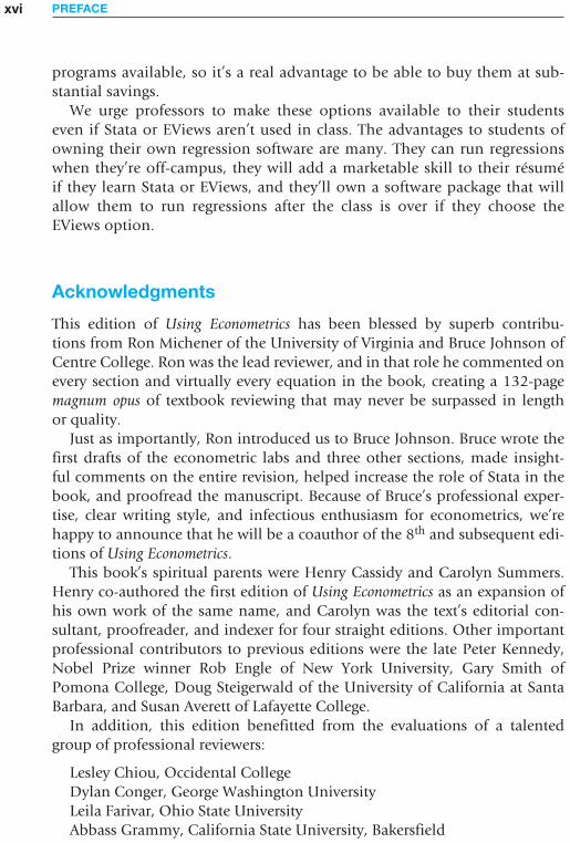
Table B-1 Critical Values of the t-Distribution
Level of Significance
Degrees of Freedom
One-Sided: 10% Two-Sided: 20%
5% 10%
2.5% 5%
1% 2%
0.5% 1%
1 3.078 6.314 12.706 31.821 63.657 2 1.886 2.920 4.303 6.965 9.925 3 1.638 2.353 3.182 4.541 5.841 4 1.533 2.132 2.776 3.747 4.604 5 1.476 2.015 2.571 3.365 4.032 6 1.440 1.943 2.447 3.143 3.707 7 1.415 1.895 2.365 2.998 3.499 8 1.397 1.860 2.306 2.896 3.355 9 1.383 1.833 2.262 2.821 3.250 10 1.372 1.812 2.228 2.764 3.169 11 1.363 1.796 2.201 2.718 3.106 12 1.356 1.782 2.179 2.681 3.055 13 1.350 1.771 2.160 2.650 3.012 14 1.345 1.761 2.145 2.624 2.977 15 1.341 1.753 2.131 2.602 2.947 16 1.337 1.746 2.120 2.583 2.921 17 1.333 1.740 2.110 2.567 2.898 18 1.330 1.734 2.101 2.552 2.878 19 1.328 1.729 2.093 2.539 2.861 20 1.325 1.725 2.086 2.528 2.845 21 1.323 1.721 2.080 2.518 2.831 22 1.321 1.717 2.074 2.508 2.819 23 1.319 1.714 2.069 2.500 2.807 24 1.318 1.711 2.064 2.492 2.797 25 1.316 1.708 2.060 2.485 2.787 26 1.315 1.706 2.056 2.479 2.779 27 1.314 1.703 2.052 2.473 2.771 28 1.313 1.701 2.048 2.467 2.763 29 1.311 1.699 2.045 2.462 2.756 30 1.310 1.697 2.042 2.457 2.750 40 1.303 1.684 2.021 2.423 2.704 60 1.296 1.671 2.000 2.390 2.660120 1.289 1.658 1.980 2.358 2.617
(Normal)∞ 1.282 1.645 1.960 2.326 2.576
Source: Reprinted from Table IV in Sir Ronald A. Fisher, Statistical Methods for Research Workers, 14th ed. (copyright © 1970, University of Adelaide) with permission of Hafner, a division of the Macmillan Publishing Company, Inc.
A02_STUD2742_07_SE_IFC.indd 1 05/02/16 4:30 PM

USING ECONOMETRICS
A01_STUD2742_07_SE_FM.indd 1 08/02/16 3:01 PM

A01_HANL4898_08_SE_FM.indd 2 24/12/14 12:49 PM
This page intentionally left blank

S E V E N T H E D I T I O N
Boston Columbus Indianapolis New York San Francisco
Amsterdam Cape Town Dubai London Madrid Milan Munich Paris Montreal Toronto
Delhi Mexico City Sao Paulo Sydney Hong Kong Seoul Singapore Taipei Tokyo
USING ECONOMETRICSA P R A C T I C A L G U I D E
A. H. StudenmundOccidental College
with the assistance of
Bruce K. JohnsonCentre College
A01_STUD2742_07_SE_FM.indd 3 08/02/16 3:01 PM

Copyright © 2017, 2011, 2006 by Pearson Education, Inc. or its affiliates. All Rights Reserved. Manufactured in the United States of America. This publication is protected by copyright, and permission should be obtained from the publisher prior to any prohibited reproduction, stor-age in a retrieval system, or transmission in any form or by any means, electronic, mechanical, photocopying, recording, or otherwise. For information regarding permissions, request forms, and the appropriate contacts within the Pearson Education Global Rights and Permissions de-partment, please visit www.pearsoned.com/permissions/.
Stata screenshots used with permission from Stata.
Acknowledgments of third-party content appear on the appropriate page within the text.
Unless otherwise indicated herein, any third-party trademarks, logos, or icons that may ap-pear in this work are the property of their respective owners, and any references to third-party trademarks, logos, icons, or other trade dress are for demonstrative or descriptive purposes only. Such references are not intended to imply any sponsorship, endorsement, authorization, or promotion of Pearson’s products by the owners of such marks, or any relationship between the owner and Pearson Education, Inc., or its affiliates, authors, licensees, or distributors.
Library of Congress Cataloging-in-Publication DataNames: Studenmund, A. H., author.Title: Using econometrics : a practical guide / A. H. Studenmund, Occidental College.Description: Seventh Edition. | Boston : Pearson, 2016. | Revised edition of the author’s Using econometrics, 2011. | Includes index.Identifiers: LCCN 2016002694 | ISBN 9780134182742Subjects: LCSH: Econometrics. | Regression analysis.Classification: LCC HB139 .S795 2016 | DDC 330.01/5195--dc23LC record available at http://lccn.loc.gov/2016002694
10 9 8 7 6 5 4 3 2 1
ISBN 10: 0-13-418274-Xwww.pearsonhighered.com ISBN 13: 978-0-13-418274-2
Vice President, Business Publishing: Donna Battista
Editor-in-Chief: Adrienne D’AmbrosioSenior Acquisitions Editor: Christina MasturzoAcquisitions Editor/Program Manager:
Neeraj BhallaEditorial Assistant: Diana TettertonVice President, Product Marketing:
Maggie MoylanDirector of Marketing, Digital Services and
Products: Jeanette KoskinasField Marketing Manager: Ramona ElmerProduct Marketing Assistant: Jessica QuazzaTeam Lead, Program Management:
Ashley SantoraTeam Lead, Project Management: Jeff HolcombProject Manager: Liz NapolitanoOperations Specialist: Carol MelvilleCreative Director: Blair Brown
Art Director: Jon BoylanVice President, Director of Digital Strategy
and Assessment: Paul GentileManager of Learning Applications:
Paul DeLucaDigital Editor: Denise ClintonDirector, Digital Studio: Sacha LaustsenDigital Studio Manager: Diane LombardoDigital Studio Project Manager: Melissa HonigDigital Studio Project Manager: Robin LazrusDigital Content Team Lead: Noel LotzDigital Content Project Lead: Courtney KamaufFull-Service Project Management and
Composition: Cenveo® Publisher ServicesInterior Designer: Cenveo® Publisher ServicesCover Designer: Jon BoylanPrinter/Binder: Edwards BrothersCover Printer: Phoenix Color/Hagerstown
A01_STUD2742_07_SE_FM.indd 4 10/02/16 9:40 AM

Dedicated to the memory of
Green Beret
Staff Sergeant
Scott Studenmund
Killed in action in Afghanistan on June 9, 2014
A01_STUD2742_07_SE_FM.indd 5 08/02/16 3:01 PM

The Pearson Series in Economics
Abel/Bernanke/Croushore Macroeconomics*
Acemoglu/Laibson/List Economics*
Bade/Parkin Foundations of Economics*
Berck/Helfand The Economics of the Environment
Bierman/Fernandez Game Theory with Economic Applications
Blanchard Macroeconomics*
Blau/Ferber/Winkler The Economics of Women, Men, and Work
Boardman/Greenberg/Vining/ Weimer Cost-Benefit Analysis
Boyer Principles of Transportation Economics
Branson Macroeconomic Theory and Policy
Bruce Public Finance and the American Economy
Carlton/Perloff Modern Industrial Organization
Case/Fair/Oster Principles of Economics*
Chapman Environmental Economics: Theory, Application, and Policy
Cooter/Ulen Law & Economics
Daniels/VanHoose International Monetary & Financial Economics
Downs An Economic Theory of Democracy
Ehrenberg/Smith Modern Labor Economics
Farnham Economics for Managers
Folland/Goodman/Stano The Economics of Health and Health Care
Fort Sports Economics
Froyen Macroeconomics
Fusfeld The Age of the Economist
Gerber International Economics*
González-Rivera Forecasting for Economics and Business
Gordon Macroeconomics*
Grant Economic Analysis of Social Issues*
Greene Econometric Analysis
Gregory Essentials of Economics
Gregory/Stuart Russian and Soviet Economic Performance and Structure
Hartwick/Olewiler The Economics of Natural Resource Use
Heilbroner/Milberg The Making of the Economic Society
Heyne/Boettke/Prychitko The Economic Way of Thinking
Holt Markets, Games, and Strategic Behavior
Hubbard/O'Brien Economics*
Money, Banking, and the Financial System*
Hubbard/O'Brien/Rafferty Macroeconomics*
Hughes/Cain American Economic History
Husted/Melvin International Economics
Jehle/Reny Advanced Microeconomic Theory
Johnson-Lans A Health Economics Primer
A01_STUD2742_07_SE_FM.indd 6 10/02/16 9:40 AM

Keat/Young/Erfle Managerial Economics
Klein Mathematical Methods for Economics
Krugman/Obstfeld/Melitz International Economics: Theory & Policy*
Laidler The Demand for Money
Leeds/von Allmen The Economics of Sports
Leeds/von Allmen/Schiming Economics*
Lynn Economic Development: Theory and Practice for a Divided World
Miller Economics Today*
Understanding Modern Economics
Miller/Benjamin The Economics of Macro Issues
Miller/Benjamin/North The Economics of Public Issues
Mills/Hamilton Urban Economics
Mishkin The Economics of Money, Banking, and Financial Markets*
The Economics of Money, Banking, and Financial Markets, Business School Edition*
Macroeconomics: Policy and Practice*
Murray Econometrics: A Modern Introduction
O'Sullivan/Sheffrin/Perez Economics: Principles, Applications and Tools*
Parkin Economics*
Perloff Microeconomics*
Microeconomics: Theory and Applications with Calculus*
Perloff/Brander Managerial Economics and Strategy*
Phelps Health Economics
Pindyck/Rubinfeld Microeconomics*
Riddell/Shackelford/Stamos/Schneider Economics: A Tool for Critically Understanding Society
Roberts The Choice: A Fable of Free Trade and Protection
Rohlf Introduction to Economic Reasoning
Roland Development Economics
Scherer Industry Structure, Strategy, and Public Policy
Schiller The Economics of Poverty and Discrimination
Sherman Market Regulation
Stock/Watson Introduction to Econometrics
Studenmund Using Econometrics: A Practical Guide
Tietenberg/Lewis Environmental and Natural Resource Economics Environmental Economics and Policy
Todaro/Smith Economic Development
Waldman/Jensen Industrial Organization: Theory and Practice
Walters/Walters/Appel/ Callahan/Centanni/ Maex/O'Neill Econversations: Today's Students Discuss Today's Issues
Weil Economic Growth
Williamson Macroeconomics
*denotes MyEconLab titles Visit www.myeconlab.com to learn more.
A01_STUD2742_07_SE_FM.indd 7 10/02/16 9:40 AM

A01_HANL4898_08_SE_FM.indd 2 24/12/14 12:49 PM
This page intentionally left blank

CONTENTS
Preface xiii
Chapter 1 An Overview of Regression Analysis 1 1.1 What Is Econometrics? 1 1.2 What Is Regression Analysis? 5 1.3 The Estimated Regression Equation 14 1.4 A Simple Example of Regression Analysis 17 1.5 Using Regression Analysis to Explain Housing Prices 20 1.6 Summary and Exercises 23 1.7 Appendix: Using Stata 30
Chapter 2 Ordinary Least Squares 35 2.1 Estimating Single-Independent-Variable
Models with OLS 35 2.2 Estimating Multivariate Regression Models with OLS 40 2.3 Evaluating the Quality of a Regression Equation 49 2.4 Describing the Overall Fit of the Estimated Model 50 2.5 An Example of the Misuse of R
2 55 2.6 Summary and Exercises 57 2.7 Appendix: Econometric Lab #1 63
Chapter 3 Learning to Use Regression Analysis 65 3.1 Steps in Applied Regression Analysis 66 3.2 Using Regression Analysis to Pick Restaurant Locations 73 3.3 Dummy Variables 79 3.4 Summary and Exercises 83 3.5 Appendix: Econometric Lab #2 89
Chapter 4 The Classical Model 92 4.1 The Classical Assumptions 92 4.2 The Sampling Distribution of βn 100 4.3 The Gauss–Markov Theorem and the Properties
of OLS Estimators 106 4.4 Standard Econometric Notation 107 4.5 Summary and Exercises 108
ix
A01_STUD2742_07_SE_FM.indd 9 08/02/16 3:01 PM

x CONTENTS
Chapter 5 Hypothesis Testing and Statistical Inference 115 5.1 What Is Hypothesis Testing? 116 5.2 The t-Test 121 5.3 Examples of t-Tests 129 5.4 Limitations of the t-Test 137 5.5 Confidence Intervals 139 5.6 The F-Test 142 5.7 Summary and Exercises 147 5.8 Appendix: Econometric Lab #3 155
Chapter 6 Specification: Choosing the Independent Variables 157
6.1 Omitted Variables 158 6.2 Irrelevant Variables 165 6.3 An Illustration of the Misuse of Specification Criteria 167 6.4 Specification Searches 169 6.5 An Example of Choosing Independent Variables 174 6.6 Summary and Exercises 177 6.7 Appendix: Additional Specification Criteria 184
Chapter 7 Specification: Choosing a Functional Form 189 7.1 The Use and Interpretation of the Constant Term 190 7.2 Alternative Functional Forms 192 7.3 Lagged Independent Variables 202 7.4 Slope Dummy Variables 203 7.5 Problems with Incorrect Functional Forms 206 7.6 Summary and Exercises 209 7.7 Appendix: Econometric Lab #4 217
Chapter 8 Multicollinearity 221 8.1 Perfect versus Imperfect Multicollinearity 222 8.2 The Consequences of Multicollinearity 226 8.3 The Detection of Multicollinearity 232 8.4 Remedies for Multicollinearity 235 8.5 An Example of Why Multicollinearity Often Is Best Left
Unadjusted 238 8.6 Summary and Exercises 240 8.7 Appendix: The SAT Interactive Regression
Learning Exercise 244
A01_STUD2742_07_SE_FM.indd 10 08/02/16 3:01 PM

xiCONTENTS
Chapter 9 Serial Correlation 273 9.1 Time Series 274 9.2 Pure versus Impure Serial Correlation 275 9.3 The Consequences of Serial Correlation 281 9.4 The Detection of Serial Correlation 284 9.5 Remedies for Serial Correlation 291 9.6 Summary and Exercises 296 9.7 Appendix: Econometric Lab #5 303
Chapter 10 Heteroskedasticity 306 10.1 Pure versus Impure Heteroskedasticity 307 10.2 The Consequences of Heteroskedasticity 312 10.3 Testing for Heteroskedasticity 314 10.4 Remedies for Heteroskedasticity 320 10.5 A More Complete Example 324 10.6 Summary and Exercises 330 10.7 Appendix: Econometric Lab #6 337
Chapter 11 Running Your Own Regression Project 340 11.1 Choosing Your Topic 341 11.2 Collecting Your Data 342 11.3 Advanced Data Sources 346 11.4 Practical Advice for Your Project 348 11.5 Writing Your Research Report 352 11.6 A Regression User’s Checklist and Guide 353 11.7 Summary 357 11.8 Appendix: The Housing Price Interactive Exercise 358
Chapter 12 Time-Series Models 364 12.1 Distributed Lag Models 365 12.2 Dynamic Models 367 12.3 Serial Correlation and Dynamic Models 371 12.4 Granger Causality 374 12.5 Spurious Correlation and Nonstationarity 376 12.6 Summary and Exercises 385
Chapter 13 Dummy Dependent Variable Techniques 390 13.1 The Linear Probability Model 390 13.2 The Binomial Logit Model 397 13.3 Other Dummy Dependent Variable Techniques 404 13.4 Summary and Exercises 406
A01_STUD2742_07_SE_FM.indd 11 08/02/16 3:01 PM

xii CONTENTS
Chapter 14 Simultaneous Equations 411 14.1 Structural and Reduced-Form Equations 412 14.2 The Bias of Ordinary Least Squares 418 14.3 Two-Stage Least Squares (2SLS) 421 14.4 The Identification Problem 430 14.5 Summary and Exercises 435 14.6 Appendix: Errors in the Variables 440
Chapter 15 Forecasting 443 15.1 What Is Forecasting? 444 15.2 More Complex Forecasting Problems 449 15.3 ARIMA Models 456 15.4 Summary and Exercises 459
Chapter 16 Experimental and Panel Data 465 16.1 Experimental Methods in Economics 466 16.2 Panel Data 473 16.3 Fixed versus Random Effects 483 16.4 Summary and Exercises 484
Appendix A Answers 491
Appendix B Statistical Tables 517
Index 531
A01_STUD2742_07_SE_FM.indd 12 08/02/16 3:01 PM

PREFACE
Econometric education is a lot like learning to fly a plane; you learn more from actually doing it than you learn from reading about it.
Using Econometrics represents an innovative approach to the understand-ing of elementary econometrics. It covers the topic of single-equation lin-ear regression analysis in an easily understandable format that emphasizes real-world examples and exercises. As the subtitle A Practical Guide implies, the book is aimed not only at beginning econometrics students but also at regression users looking for a refresher and at experienced practitioners who want a convenient reference.
What’s New in the Seventh Edition?
Using Econometrics has been praised as “one of the most important new texts of the last 30 years,” so we’ve retained the clarity and practicality of previous editions. However, we’re delighted to have made a number of substantial improvements in the text.
The most exciting upgrades are:
1. Econometric Labs: These new and innovative learning tools are optional appendices that give students hands-on opportunities to bet-ter understand the econometric principles that they’re reading about in the chapters. The labs originally were designed to be assigned in a classroom setting, but they also have turned out to be extremely valu-able for readers who are not in a class or for individual students in classes where the labs aren’t assigned. Hints on how best to use these econometric labs and answers to the lab questions are available in the instructor’s manual on the Using Econometrics Web site.
2. The Use of Stata throughout the Text: In our opinion, Stata has become the econometric software package of choice among economic researchers. As a result, we have estimated all the text examples and exercises with Stata and have included a short appendix to help stu-dents get started with Stata. Beyond this, we have added a complete guide to Using Stata to our Web site. This guide, written by John Perry of Centre College, explains in detail all the Stata commands needed to replicate the text’s equations and answer the text’s exercises. However, even though we use Stata extensively, Using Econometrics is not tied to
xiii
A01_STUD2742_07_SE_FM.indd 13 08/02/16 3:01 PM

Stata or any other econometric software, so the text works well with all standard regression packages.
3. Expanded Econometric Content: We have added coverage of a number of econometric tests and procedures, for example the Breusch-Pagan test and the Prais–Winsten approach to Generalized Least Squares. In addition, we have expanded the coverage of even more topics, for example the F-test, confidence intervals, the Lagrange Multiplier test, and the Dickey–Fuller test. Finally, we have simplified the notation and improved the clarity of the explanations in Chapters 12–16, particu-larly in topics like dynamic equations, dummy dependent variables, instrumental variables, and panel data.
4. Answers to Many More Exercises: In response to requests from instruc-tors and students, we have more than tripled the number of exercises that are answered in the text’s appendix. These answers will allow stu-dents to learn on their own, because students will be able to attempt an exercise and then check their answers against those in the back of the book without having to involve their professors. In order to continue to provide good exercises for professors to include in problem sets and exams, we have expanded the number of exercises contained in the text’s Web site.
5. Dramatically Improved PowerPoint Slides: We recognize the impor-tance of PowerPoint slides to instructors with large classes, so we have dramatically improved the quality of the text’s PowerPoints. The slides replicate each chapter’s main equations and examples, and also pro-vide chapter summaries and lists of the key concepts in each chapter. The PowerPoint slides can be downloaded from the text’s Web site, and they’re designed to be easily edited and individualized.
6. An Expanded and Improved Web Site: We believe that this edition’s Web site is the best we’ve produced. As you’d expect, the Web site includes all the text’s data sets, in easily downloadable Stata, EViews, Excel, and ASCII formats, but we have gone far beyond that. We have added Using Stata, a complete guide to the Stata commands needed to estimate the book’s equations; we have dramatically improved the PowerPoint slides; and we have added answers to the new economet-ric labs and instructions on how best to use these labs in a classroom setting. In addition, the Web site also includes an instructor’s manual, additional exercises, extra interactive regression learning exercises, and additional data sets. But why take our word for it? Take a look for your-self at http://www.pearsonhighered.com/studenmund
xiv PREFACE
A01_STUD2742_07_SE_FM.indd 14 08/02/16 3:01 PM

Features
1. Our approach to the learning of econometrics is simple, intuitive, and easy to understand. We do not use matrix algebra, and we relegate proofs and calculus to the footnotes or exercises.
2. We include numerous examples and example-based exercises. We feel that the best way to get a solid grasp of applied econometrics is through an example-oriented approach.
3. Although most of this book is at a simpler level than other economet-rics texts, Chapters 6 and 7 on specification choice are among the most complete in the field. We think that an understanding of specification issues is vital for regression users.
4. We use a unique kind of learning tool called an interactive regression learning exercise to help students simulate econometric analysis by giving them feedback on various kinds of decisions without relying on computer time or much instructor supervision.
5. We’re delighted to introduce a new innovative learning tool called an econometric lab. These econometric labs, developed by Bruce Johnson of Centre College and tested successfully at two other institutions, are optional appendices aimed at giving students hands-on experi-ence with the econometric procedures they’re reading about. Students who complete these econometric labs will be much better prepared to undertake econometric research on their own.
The formal prerequisites for using this book are few. Readers are assumed to have been exposed to some microeconomic and macroeconomic theory, basic mathematical functions, and elementary statistics (even if they have forgotten most if it). Students with little statistical background are encour-aged to begin their study of econometrics by reading Chapter 17, “Statistical Principles,” on the text’s Web site.
Because the prerequisites are few and the statistics material is self-contained, Using Econometrics can be used not only in undergraduate courses but also in MBA-level courses in quantitative methods. We also have been told that the book is a helpful supplement for graduate-level econometrics courses.
The Stata and EViews Options
We’re delighted to be able to offer our readers the chance to purchase the student version of Stata or EViews at discounted prices when bundled with the textbook. Stata and EViews are two of the best econometric software
xvPREFACE
A01_STUD2742_07_SE_FM.indd 15 08/02/16 3:01 PM
programs available, so it’s a real advantage to be able to buy them at sub-stantial savings.
We urge professors to make these options available to their students even if Stata or EViews aren’t used in class. The advantages to students of owning their own regression software are many. They can run regressions when they’re off-campus, they will add a marketable skill to their résumé if they learn Stata or EViews, and they’ll own a software package that will allow them to run regressions after the class is over if they choose the EViews option.
Acknowledgments
This edition of Using Econometrics has been blessed by superb contribu-tions from Ron Michener of the University of Virginia and Bruce Johnson of Centre College. Ron was the lead reviewer, and in that role he commented on every section and virtually every equation in the book, creating a 132-page magnum opus of textbook reviewing that may never be surpassed in length or quality.
Just as importantly, Ron introduced us to Bruce Johnson. Bruce wrote the first drafts of the econometric labs and three other sections, made insight-ful comments on the entire revision, helped increase the role of Stata in the book, and proofread the manuscript. Because of Bruce’s professional exper-tise, clear writing style, and infectious enthusiasm for econometrics, we’re happy to announce that he will be a coauthor of the 8th and subsequent edi-tions of Using Econometrics.
This book’s spiritual parents were Henry Cassidy and Carolyn Summers. Henry co-authored the first edition of Using Econometrics as an expansion of his own work of the same name, and Carolyn was the text’s editorial con-sultant, proofreader, and indexer for four straight editions. Other important professional contributors to previous editions were the late Peter Kennedy, Nobel Prize winner Rob Engle of New York University, Gary Smith of Pomona College, Doug Steigerwald of the University of California at Santa Barbara, and Susan Averett of Lafayette College.
In addition, this edition benefitted from the evaluations of a talented group of professional reviewers:
Lesley Chiou, Occidental CollegeDylan Conger, George Washington UniversityLeila Farivar, Ohio State UniversityAbbass Grammy, California State University, Bakersfield
xvi PREFACE
A01_STUD2742_07_SE_FM.indd 16 08/02/16 3:01 PM

Jason Hecht, Ramapo CollegeJin Man Lee, University of Illinois at ChicagoNoelwah Netusl, Reed CollegeRobert Parks, Washington University in St. LouisDavid Phillips, Hope CollegeJohn Perry, Centre CollegeRobert Shapiro, Columbia UniversityPhanindra Wunnava, Middlebury College
Invaluable in the editorial and production process were Jean Berming-ham, Neeraj Bhalla, Adrienne D’Ambrosio, Marguerite Dessornes, Christina Masturzo, Liz Napolitano, Bill Rising, and Kathy Smith. Providing crucial emotional support during an extremely difficult time were Sarah Newhall, Barbara Passerelle, Barbara and David Studenmund, and my immediate family, Jaynie and Connell Studenmund and Brent Morse. Finally, I’d like to thank my wonderful Occidental College colleagues and students for their feedback and encouragement. These particularly included Lesley Chiou, Jack Gephart, Jorge Gonzalez, Andy Jalil, Kate Johnstone, Mary Lopez, Jessica May, Cole Moniz, Robby Moore, Kyle Yee, and, especially, Koby Deitz.
A. H. Studenmund
xviiPREFACE
A01_STUD2742_07_SE_FM.indd 17 08/02/16 3:01 PM

A01_HANL4898_08_SE_FM.indd 2 24/12/14 12:49 PM
This page intentionally left blank
1
1.1 What Is Econometrics?
1.2 What Is Regression Analysis?
1.3 The Estimated Regression Equation
1.4 A Simple Example of Regression Analysis
1.5 Using Regression to Explain Housing Prices
1.6 Summary and Exercises
1.7 Appendix: Using Stata
An Overview of Regression Analysis
1.1 What Is Econometrics?
“ Econometrics is too mathematical; it’s the reason my best friend isn’t majoring in economics.”
“ There are two things you are better off not watching in the making: sausages and econometric estimates.”1
“ Econometrics may be defined as the quantitative analysis of actual economic phenomena.”2
“ It’s my experience that ‘economy-tricks’ is usually nothing more than a justification of what the author believed before the research was begun.”
Obviously, econometrics means different things to different people. To beginning students, it may seem as if econometrics is an overly complex obstacle to an otherwise useful education. To skeptical observers, econometric
Chapter 1
1. Ed Leamer, “Let’s take the Con out of Econometrics,” American Economic Review, Vol. 73, No. 1, p. 37.
2. Paul A. Samuelson, T. C. Koopmans, and J. R. Stone, “Report of the Evaluative Committee for Econometrica,” Econometrica, 1954, p. 141.
M01_STUD2742_07_SE_C01.indd 1 1/4/16 4:54 PM

2 CHAPTER 1 An Overview Of regressiOn AnAlysis
results should be trusted only when the steps that produced those results are completely known. To professionals in the field, econometrics is a fascinat-ing set of techniques that allows the measurement and analysis of economic phenomena and the prediction of future economic trends.
You’re probably thinking that such diverse points of view sound like the statements of blind people trying to describe an elephant based on which part they happen to be touching, and you’re partially right. Econometrics has both a formal definition and a larger context. Although you can easily memorize the formal definition, you’ll get the complete picture only by understanding the many uses of and alternative approaches to econometrics.
That said, we need a formal definition. Econometrics—literally, “economic measurement”—is the quantitative measurement and analysis of actual economic and business phenomena. It attempts to quantify economic reality and bridge the gap between the abstract world of economic theory and the real world of human activity. To many students, these worlds may seem far apart. On the one hand, economists theorize equilibrium prices based on carefully conceived marginal costs and marginal revenues; on the other, many firms seem to operate as though they have never heard of such concepts. Econometrics allows us to examine data and to quantify the actions of firms, consumers, and governments. Such measurements have a number of different uses, and an examination of these uses is the first step to understanding econometrics.
Uses of Econometrics
Econometrics has three major uses:
1. describing economic reality
2. testing hypotheses about economic theory and policy
3. forecasting future economic activity
The simplest use of econometrics is description. We can use econometrics to quantify economic activity and measure marginal effects because econo-metrics allows us to estimate numbers and put them in equations that previ-ously contained only abstract symbols. For example, consumer demand for a particular product often can be thought of as a relationship between the quantity demanded 1Q2 and the product’s price 1P2, the price of a substitute 1Ps2, and disposable income 1Yd2. For most goods, the relationship between consumption and disposable income is expected to be positive, because an increase in disposable income will be associated with an increase in the consumption of the product. Econometrics actually allows us to estimate that
M01_STUD2742_07_SE_C01.indd 2 1/4/16 4:54 PM

3 whAt is ecOnOmetrics?
relationship based upon past consumption, income, and prices. In other words, a general and purely theoretical functional relationship like:
Q = β0 + β1P + β2PS + β1Yd (1.1)
can become explicit:
Q = 27.7 - 0.11P + 0.03PS + 0.23Yd (1.2)
This technique gives a much more specific and descriptive picture of the function.3 Let’s compare Equations 1.1 and 1.2. Instead of expecting con-sumption merely to “increase” if there is an increase in disposable income, Equation 1.2 allows us to expect an increase of a specific amount (0.23 units for each unit of increased disposable income). The number 0.23 is called an estimated regression coefficient, and it is the ability to estimate these coeffi-cients that makes econometrics valuable.
The second use of econometrics is hypothesis testing, the evaluation of alternative theories with quantitative evidence. Much of economics involves building theoretical models and testing them against evidence, and hypoth-esis testing is vital to that scientific approach. For example, you could test the hypothesis that the product in Equation 1.1 is what economists call a normal good (one for which the quantity demanded increases when disposable income increases). You could do this by applying various statistical tests to the estimated coefficient (0.23) of disposable income (Yd) in Equation 1.2. At first glance, the evidence would seem to support this hypothesis, because the coefficient’s sign is positive, but the “statistical significance” of that estimate would have to be investigated before such a conclusion could be justified. Even though the estimated coefficient is positive, as expected, it may not be sufficiently different from zero to convince us that the true coefficient is indeed positive.
The third and most difficult use of econometrics is to forecast or predict what is likely to happen next quarter, next year, or further into the future, based on what has happened in the past. For example, economists use economet-ric models to make forecasts of variables like sales, profits, Gross Domestic Product (GDP), and the inflation rate. The accuracy of such forecasts depends in large measure on the degree to which the past is a good guide to the future. Business leaders and politicians tend to be especially interested in this use of
3. It’s of course naïve to build a model of sales (demand) without taking supply into consider-ation. Unfortunately, it’s very difficult to learn how to estimate a system of simultaneous equa-tions until you’ve learned how to estimate a single equation. As a result, we will postpone our discussion of the econometrics of simultaneous equations until Chapter 14. Until then, you should be aware that we sometimes will encounter right-hand-side variables that are not truly “independent” from a theoretical point of view.
M01_STUD2742_07_SE_C01.indd 3 1/4/16 4:54 PM

4 CHAPTER 1 An Overview Of regressiOn AnAlysis
econometrics because they need to make decisions about the future, and the penalty for being wrong (bankruptcy for the entrepreneur and political defeat for the candidate) is high. To the extent that econometrics can shed light on the impact of their policies, business and government leaders will be better equipped to make decisions. For example, if the president of a company that sold the product modeled in Equation 1.1 wanted to decide whether to increase prices, forecasts of sales with and without the price increase could be calculated and compared to help make such a decision.
Alternative Econometric Approaches
There are many different approaches to quantitative work. For example, the fields of biology, psychology, and physics all face quantitative questions simi-lar to those faced in economics and business. However, these fields tend to use somewhat different techniques for analysis because the problems they face aren’t the same. For example, economics typically is an observational disci-pline rather than an experimental one. “We need a special field called econo-metrics, and textbooks about it, because it is generally accepted that economic data possess certain properties that are not considered in standard statistics texts or are not sufficiently emphasized there for use by economists.”4
Different approaches also make sense within the field of economics. A model built solely for descriptive purposes might be different from a forecast-ing model, for example.
To get a better picture of these approaches, let’s look at the steps used in nonexperimental quantitative research:
1. specifying the models or relationships to be studied
2. collecting the data needed to quantify the models
3. quantifying the models with the data
The specifications used in step 1 and the techniques used in step 3 differ widely between and within disciplines. Choosing the best specification for a given model is a theory-based skill that is often referred to as the “art” of econometrics. There are many alternative approaches to quantifying the same equation, and each approach may produce somewhat different results. The choice of approach is left to the individual econometrician (the researcher using econometrics), but each researcher should be able to justify that choice.
4. Clive Granger, “A Review of Some Recent Textbooks of Econometrics,” Journal of Economic Literature, Vol. 32, No. 1, p. 117.
M01_STUD2742_07_SE_C01.indd 4 1/4/16 4:54 PM

5 whAt is regressiOn AnAlysis?
This book will focus primarily on one particular econometric approach: single-equation linear regression analysis. The majority of this book will thus concentrate on regression analysis, but it is important for every econometri-cian to remember that regression is only one of many approaches to econo-metric quantification.
The importance of critical evaluation cannot be stressed enough; a good econometrician can diagnose faults in a particular approach and figure out how to repair them. The limitations of the regression analysis approach must be fully perceived and appreciated by anyone attempting to use regression analysis or its findings. The possibility of missing or inaccurate data, incor-rectly formulated relationships, poorly chosen estimating techniques, or improper statistical testing procedures implies that the results from regres-sion analyses always should be viewed with some caution.
1.2 What Is Regression Analysis?
Econometricians use regression analysis to make quantitative estimates of economic relationships that previously have been completely theoretical in nature. After all, anybody can claim that the quantity of iPhones demanded will increase if the price of those phones decreases (holding everything else constant), but not many people can put specific numbers into an equation and estimate by how many iPhones the quantity demanded will increase for each dollar that price decreases. To predict the direction of the change, you need a knowledge of economic theory and the general characteristics of the product in question. To predict the amount of the change, though, you need a sample of data, and you need a way to estimate the relationship. The most frequently used method to estimate such a relationship in econometrics is regression analysis.
Dependent Variables, Independent Variables, and Causality
Regression analysis is a statistical technique that attempts to “explain” move-ments in one variable, the dependent variable, as a function of movements in a set of other variables, called the independent (or explanatory) variables, through the quantification of one or more equations. For example, in Equation 1.1:
Q = β0 + β1P + β2PS + β1Yd (1.1)
Q is the dependent variable and P, PS, and Yd are the independent variables. Regression analysis is a natural tool for economists because most (though not all) economic propositions can be stated in such equations. For example, the quantity demanded (dependent variable) is a function of price, the prices of substitutes, and income (independent variables).
M01_STUD2742_07_SE_C01.indd 5 1/4/16 4:54 PM
6 CHAPTER 1 An Overview Of regressiOn AnAlysis
Much of economics and business is concerned with cause-and-effect propositions. If the price of a good increases by one unit, then the quantity demanded decreases on average by a certain amount, depending on the price elasticity of demand (defined as the percentage change in the quantity demanded that is caused by a one percent increase in price). Similarly, if the quantity of capital employed increases by one unit, then output increases by a certain amount, called the marginal productivity of capital. Propositions such as these pose an if-then, or causal, relationship that logically postulates that a dependent variable’s movements are determined by movements in a number of specific independent variables.
Don’t be deceived by the words “dependent” and “independent,” how-ever. Although many economic relationships are causal by their very nature, a regression result, no matter how statistically significant, cannot prove causality. All regression analysis can do is test whether a signifi-cant quantitative relationship exists. Judgments as to causality must also include a healthy dose of economic theory and common sense. For example, the fact that the bell on the door of a flower shop rings just be-fore a customer enters and purchases some flowers by no means implies that the bell causes purchases! If events A and B are related statistically, it may be that A causes B, that B causes A, that some omitted factor causes both, or that a chance correlation exists between the two.
The cause-and-effect relationship often is so subtle that it fools even the most prominent economists. For example, in the late nineteenth century, English economist Stanley Jevons hypothesized that sunspots caused an increase in economic activity. To test this theory, he collected data on national output (the dependent variable) and sunspot activity (the independent variable) and showed that a significant positive relationship existed. This result led him, and some others, to jump to the conclusion that sunspots did indeed cause output to rise. Such a conclusion was unjustified because regression analysis cannot confirm causality; it can only test the strength and direction of the quantitative relationships involved.
Single-Equation Linear Models
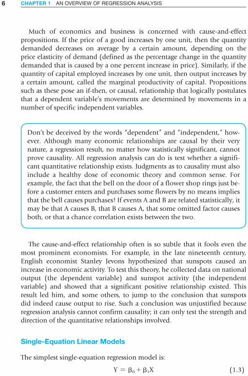
The simplest single-equation regression model is:
Y = β0 + β1X (1.3)
M01_STUD2742_07_SE_C01.indd 6 1/4/16 4:54 PM

7 whAt is regressiOn AnAlysis?
Equation 1.3 states that Y, the dependent variable, is a single-equation linear function of X, the independent variable. The model is a single-equation model because it’s the only equation specified. The model is linear because if you were to plot Equation 1.3 it would be a straight line rather than a curve.
The βs are the coefficients that determine the coordinates of the straight line at any point. β0 is the constant or intercept term; it indicates the value of Y when X equals zero. β1 is the slope coefficient, and it indicates the amount that Y will change when X increases by one unit. The line in Figure 1.1 illustrates the relationship between the coefficients and the graphical meaning of the regres-sion equation. As can be seen from the diagram, Equation 1.3 is indeed linear.
The slope coefficient, β1, shows the response of Y to a one-unit increase in X. Much of the emphasis in regression analysis is on slope coefficients such as β1. In Figure 1.1 for example, if X were to increase by one from X1 to X2 1∆X2, the value of Y in Equation 1.3 would increase from Y1 to Y2 1∆Y2. For linear (i.e., straight-line) regression models, the response in the predicted value of Y due to a change in X is constant and equal to the slope coefficient β1:
1Y2 - Y121X2 - X12 =
∆Y∆X
= β1
Y
Y2
Intercept = d0
Y1
0 X1
¢X
¢Y
X2
Y = d0 + d1X
X
¢Y¢X
Slope = d1 = (Y2 - Y1)(X2 - X1)
=
Figure 1.1 graphical representation of the coefficients of the regression line
The graph of the equation Y = β0 + β1X is linear with a constant slope equal to β1 = ∆Y/∆X.
M01_STUD2742_07_SE_C01.indd 7 1/4/16 4:54 PM

8 CHAPTER 1 An Overview Of regressiOn AnAlysis
where ∆ is used to denote a change in the variables. Some readers may recog-nize this as the “rise” 1∆Y2 divided by the “run” 1∆X2. For a linear model, the slope is constant over the entire function.
If linear regression techniques are going to be applied to an equation, that equation must be linear. An equation is linear if plotting the function in terms of X and Y generates a straight line; for example, Equation 1.3 is linear.5
Y = β0 + β1X (1.3)
The Stochastic Error Term
Besides the variation in the dependent variable (Y) that is caused by the independent variable (X), there is almost always variation that comes from other sources as well. This additional variation comes in part from omitted explanatory variables (e.g., X2 and X3). However, even if these extra variables are added to the equation, there still is going to be some variation in Y that simply cannot be explained by the model.6 This variation probably comes from sources such as omitted influences, measurement error, incorrect func-tional form, or purely random and totally unpredictable occurrences. By random we mean something that has its value determined entirely by chance.
Econometricians admit the existence of such inherent unexplained varia-tion (“error”) by explicitly including a stochastic (or random) error term in their regression models. A stochastic error term is a term that is added to a regression equation to introduce all of the variation in Y that cannot be explained by the included Xs. It is, in effect, a symbol of the econometrician’s ignorance or inability to model all the movements of the dependent variable. The error term (sometimes called a disturbance term) usually is referred to with the symbol epsilon 1e2, although other symbols (like u or v) sometimes are used.
5. Technically, as you will learn in Chapter 7, this equation is linear in the coefficients β0 and β1 and linear in the variables Y and X. The application of regression analysis to equations that are nonlinear in the variables is covered in Chapter 7. The application of regression techniques to equations that are nonlinear in the coefficients, however, is much more difficult.
6. The exception would be the extremely rare case where the data can be explained by some sort of physical law and are measured perfectly. Here, continued variation would point to an omitted independent variable. A similar kind of problem is often encountered in astronomy, where planets can be discovered by noting that the orbits of known planets exhibit variations that can be caused only by the gravitational pull of another heavenly body. Absent these kinds of physi-cal laws, researchers in economics and business would be foolhardy to believe that all variation in Y can be explained by a regression model because there are always elements of error in any attempt to measure a behavioral relationship.
M01_STUD2742_07_SE_C01.indd 8 1/4/16 4:54 PM

9 whAt is regressiOn AnAlysis?
The addition of a stochastic error term 1e2 to Equation 1.3 results in a typical regression equation:
Y = β0 + β1X + e (1.4)
Equation 1.4 can be thought of as having two components, the deterministic component and the stochastic, or random, component. The expression β0 + β1X is called the deterministic component of the regression equation because it indicates the value of Y that is determined by a given value of X, which is assumed to be nonstochastic. This deterministic component can also be thought of as the expected value of Y given X, the mean value of the Ys associated with a particular value of X. For example, if the average height of all 13-year-old girls is 5 feet, then 5 feet is the expected value of a girl’s height given that she is 13. The deterministic part of the equation may be written:
E1Y � X2 = β0 + β1X (1.5)
which states that the expected value of Y given X, denoted as E1Y � X2, is a linear function of the independent variable (or variables if there are more than one).
Unfortunately, the value of Y observed in the real world is unlikely to be exactly equal to the deterministic expected value E1Y � X2. After all, not all 13-year-old girls are 5 feet tall. As a result, the stochastic element 1e2 must be added to the equation:
Y = E1Y � X2 + e = β0 + β1X + e (1.6)
The stochastic error term must be present in a regression equation because there are at least four sources of variation in Y other than the variation in the included Xs:
1. Many minor influences on Y are omitted from the equation (for example, because data are unavailable).
2. It is virtually impossible to avoid some sort of measurement error in the dependent variable.
3. The underlying theoretical equation might have a different functional form (or shape) than the one chosen for the regression. For example, the underlying equation might be nonlinear.
4. All attempts to generalize human behavior must contain at least some amount of unpredictable or purely random variation.
M01_STUD2742_07_SE_C01.indd 9 1/4/16 4:55 PM

10 Chapter 1 An Overview Of regressiOn AnAlysis
To get a better feeling for these components of the stochastic error term, let’s think about a consumption function (aggregate consumption as a func-tion of aggregate disposable income). First, consumption in a particular year may have been less than it would have been because of uncertainty over the future course of the economy. Since this uncertainty is hard to measure, there might be no variable measuring consumer uncertainty in the equation. In such a case, the impact of the omitted variable (consumer uncertainty) would likely end up in the stochastic error term. Second, the observed amount of consumption may have been different from the actual level of consump-tion in a particular year due to an error (such as a sampling error) in the measurement of consumption in the National Income Accounts. Third, the underlying consumption function may be nonlinear, but a linear consump-tion function might be estimated. (To see how this incorrect functional form would cause errors, see Figure 1.2.) Fourth, the consumption function
Y
0
Errors
“True” Relationship(nonlinear)
Linear Functional Form
X
g2
g1
g3
Figure 1.2 errors Caused by Using a linear functional form to Model a nonlinear relationship
One source of stochastic error is the use of an incorrect functional form. For example, if a linear functional form is used when the underlying relationship is nonlinear, systematic errors (the es) will occur. These nonlinearities are just one component of the stochastic error term. The others are omitted variables, measurement error, and purely random variation.
M01_STUD2742_07_SE_C01.indd 10 19/01/16 4:50 PM

11 whAt is regressiOn AnAlysis?
attempts to portray the behavior of people, and there is always an element of unpredictability in human behavior. At any given time, some random event might increase or decrease aggregate consumption in a way that might never be repeated and couldn’t be anticipated.
These possibilities explain the existence of a difference between the observed values of Y and the values expected from the deterministic com-ponent of the equation, E1Y � X2. These sources of error will be covered in more detail in the following chapters, but for now it is enough to recognize that in econometric research there will always be some stochastic or random element, and, for this reason, an error term must be added to all regression equations.
Extending the Notation
Our regression notation needs to be extended to allow the possibility of more than one independent variable and to include reference to the number of observations. A typical observation (or unit of analysis) is an individual person, year, or country. For example, a series of annual observations starting in 1985 would have Y1 = Y for 1985, Y2 for 1986, etc. If we include a specific reference to the observations, the single-equation linear regression model may be written as:
Yi = β0 + β1Xi + ei 1i = 1, 2, c, N2 (1.7)
where: Yi = the ith observation of the dependent variable Xi = the ith observation of the independent variable ei = the ith observation of the stochastic error term β0, β1 = the regression coefficients N = the number of observations
This equation is actually N equations, one for each of the N observations:
Y1 = β0 + β1X1 + e1
Y2 = β0 + β1X2 + e2
Y3 = β0 + β1X3 + e3
f YN = β0 + β1XN + eN
That is, the regression model is assumed to hold for each observation. The coefficients do not change from observation to observation, but the values of Y, X, and e do.
M01_STUD2742_07_SE_C01.indd 11 1/4/16 4:55 PM

12 CHAPTER 1 An Overview Of regressiOn AnAlysis
A second notational addition allows for more than one independent vari-able. Since more than one independent variable is likely to have an effect on the dependent variable, our notation should allow these additional explana-tory Xs to be added. If we define:
X1i = the ith observation of the first independent variableX2i = the ith observation of the second independent variableX3i = the ith observation of the third independent variable
then all three variables can be expressed as determinants of Y.
The resulting equation is called a multivariate (more than one indepen-dent variable) linear regression model:
Yi = β0 + β1X1i + β2X2i + β3X3i + ei (1.8)
The meaning of the regression coefficient β1 in this equation is the impact of a one-unit increase in X1 on the dependent variable Y, holding constant X2 and X3. Similarly, β2 gives the impact of a one-unit increase in X2 on Y, holding X1 and X3 constant.
These multivariate regression coefficients (which are parallel in nature to partial derivatives in calculus) serve to isolate the impact on Y of a change in one variable from the impact on Y of changes in the other variables. This is possible because multivariate regression takes the movements of X2 and X3 into account when it estimates the coefficient of X1. The result is quite similar to what we would obtain if we were capable of conducting controlled labora-tory experiments in which only one variable at a time was changed.
In the real world, though, it is very difficult to run controlled economic experiments,7 because many economic factors change simultaneously, often in opposite directions. Thus the ability of regression analysis to measure the impact of one variable on the dependent variable, holding constant the influence of the other variables in the equation, is a tremendous advantage. Note that if a variable is not included in an equation, then its impact is not held constant in the estimation of the regression coefficients. This will be discussed further in Chapter 6.
7. Such experiments are difficult but not impossible. See Section 16.1.
M01_STUD2742_07_SE_C01.indd 12 1/4/16 4:55 PM

13 whAt is regressiOn AnAlysis?
This material is pretty abstract, so let’s look at two examples. As a first example, consider an equation with only one independent variable, a model of a person’s weight as a function of their height. The theory behind this equation is that, other things being equal, the taller a person is the more they tend to weigh.
The dependent variable in such an equation would be the weight of the person, while the independent variable would be that person’s height:
Weighti = β0 + β1Heighti + ei (1.9)
What exactly do the “i” subscripts mean in Equation 1.9? Each value of i refers to a different person in the sample, so another way to think about the subscripts is that:
Weightwoody = β0 + β1Heightwoody + ewoody
Weightlesley = β0 + β1Heightlesley + elesley
Weightbruce = β0 + β1Heightbruce + ebruce
Weightmary = β0 + β1Heightmary + emary
Take a look at these equations. Each person (observation) in the sample has their own individual weight and height; that makes sense. But why does each person have their own value for e, the stochastic error term? The answer is that random events (like those expressed by e) impact people differently, so each person needs to have their own value of e in order to reflect these differences. In contrast, note that the subscripts of the regression coefficients (the βs) don’t change from person to person but instead apply to the entire sample. We’ll learn more about this equation in Section 1.4.
As a second example, let’s look at an equation with more than one inde-pendent variable. Suppose we want to understand how wages are determined in a particular field, perhaps because we think that there might be discrimi-nation in that field. The wage of a worker would be the dependent variable (WAGE), but what would be good independent variables? What variables would influence a person’s wage in a given field? Well, there are literally doz-ens of reasonable possibilities, but three of the most common are the work experience (EXP), education (EDU), and gender (GEND) of the worker, so let’s use these. To create a regression equation with these variables, we’d rede-fine the variables in Equation 1.8 to meet our definitions:
Y = WAGE = the wage of the workerX1 = EXP = the years of work experience of the workerX2 = EDU = the years of education beyond high school of the workerX3 = GEND = the gender of the worker (1 = male and 0 = female)
M01_STUD2742_07_SE_C01.indd 13 1/4/16 4:55 PM

14 CHAPTER 1 An Overview Of regressiOn AnAlysis
The last variable, GEND, is unusual in that it can take on only two values, 0 and 1; this kind of variable is called a dummy variable, and it’s extremely useful when we want to quantify a concept that is inherently qualitative (like gender). We’ll discuss dummy variables in more depth in Sections 3.3 and 7.4.
If we substitute these definitions into Equation 1.8, we get:
WAGEi = β0 + β1EXPi + β2EDUi + β3GENDi + ei (1.10)
Equation 1.10 specifies that a worker’s wage is a function of the experience, education, and gender of that worker. In such an equation, what would the meaning of β1 be? Some readers will guess that β1 measures the amount by which the average wage increases for an additional year of experience, but such a guess would miss the fact that there are two other independent vari-ables in the equation that also explain wages. The correct answer is that β1
gives us the impact on wages of a one-year increase in experience, holding con-stant education and gender. This is a significant difference, because it allows researchers to control for specific complicating factors without running con-trolled experiments.
Before we conclude this section, it’s worth noting that the general multi-variate regression model with K independent variables is written as:
Yi = β0 + β1X1i + β2X2i + g + βKXKi + ei (1.11)
where i goes from 1 to N and indicates the observation number.If the sample consists of a series of years or months (called a time series),
then the subscript i is usually replaced with a t to denote time.8
1.3 The Estimated Regression Equation
Once a specific equation has been decided upon, it must be quantified. This quantified version of the theoretical regression equation is called the esti-mated regression equation and is obtained from a sample of data for actual Xs and Ys. Although the theoretical equation is purely abstract in nature:
Yi = β0 + β1Xi + ei (1.12)
8. The order of the subscripts doesn’t matter as long as the appropriate definitions are presented. We prefer to list the variable number first 1X1i2 because we think it’s easier for a beginning econometrician to understand. However, as the reader moves on to matrix algebra and com-puter spreadsheets, it will become common to list the observation number first, as in Xi1. Often the observational subscript is deleted, and the reader is expected to understand that the equation holds for each observation in the sample.
M01_STUD2742_07_SE_C01.indd 14 1/4/16 4:55 PM
15 the estimAted regressiOn eqUAtiOn
the estimated regression equation has actual numbers in it:
YN i = 103.40 + 6.38Xi (1.13)
The observed, real-world values of X and Y are used to calculate the coef-ficient estimates 103.40 and 6.38. These estimates are used to determine YN (read as “Y-hat”), the estimated or fitted value of Y.
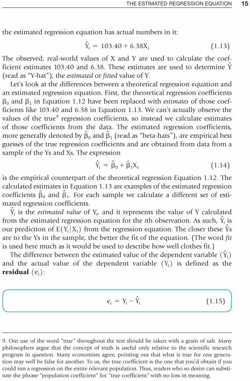
Let’s look at the differences between a theoretical regression equation and an estimated regression equation. First, the theoretical regression coefficients β0 and β1 in Equation 1.12 have been replaced with estimates of those coef-ficients like 103.40 and 6.38 in Equation 1.13. We can’t actually observe the values of the true9 regression coefficients, so instead we calculate estimates of those coefficients from the data. The estimated regression coefficients, more generally denoted by βN 0 and βN 1 (read as “beta-hats”), are empirical best guesses of the true regression coefficients and are obtained from data from a sample of the Ys and Xs. The expression
YN i = βN 0 + βN 1Xi (1.14)
is the empirical counterpart of the theoretical regression Equation 1.12. The calculated estimates in Equation 1.13 are examples of the estimated regression coefficients βN 0 and βN 1. For each sample we calculate a different set of esti-mated regression coefficients.
YN i is the estimated value of Yi, and it represents the value of Y calculated from the estimated regression equation for the ith observation. As such, YN i is our prediction of E1Yi � Xi2 from the regression equation. The closer these YN s are to the Ys in the sample, the better the fit of the equation. (The word fit is used here much as it would be used to describe how well clothes fit.)
The difference between the estimated value of the dependent variable 1YN i2 and the actual value of the dependent variable 1Yi2 is defined as the residual 1ei2:
9. Our use of the word “true” throughout the text should be taken with a grain of salt. Many philosophers argue that the concept of truth is useful only relative to the scientific research program in question. Many economists agree, pointing out that what is true for one genera-tion may well be false for another. To us, the true coefficient is the one that you’d obtain if you could run a regression on the entire relevant population. Thus, readers who so desire can substi-tute the phrase “population coefficient” for “true coefficient” with no loss in meaning.
ei = Yi - YN i (1.15)
M01_STUD2742_07_SE_C01.indd 15 1/4/16 4:55 PM

16 CHAPTER 1 An Overview Of regressiOn AnAlysis
Note the distinction between the residual in Equation 1.15 and the error term:
ei = Yi - E1Yi � Xi2 (1.16)
The residual is the difference between the observed Y and the estimated regres-sion line 1YN 2, while the error term is the difference between the observed Y and the true regression equation (the expected value of Y). Note that the error term is a theoretical concept that can never be observed, but the residual is a real-world value that is calculated for each observation every time a regression is run. The residual can be thought of as an estimate of the error term, and e could have been denoted as eN. Most regression techniques not only calculate the residuals but also attempt to compute values of βN 0 and βN 1 that keep the residuals as low as possible. The smaller the residuals, the better the fit, and the closer the YN s will be to the Ys.
All these concepts are shown in Figure 1.3. The 1X, Y2 pairs are shown as points on the diagram, and both the true regression equation (which
g6
Y
Y6
0 X6
Yi = d0 + d1Xi(Estimated Line)
E(Yi|Xi) = d0 + d1Xi(True Line)
X
d0
Y6
e6e6
d0
N
N
N N N
Figure 1.3 true and estimated regression lines
The true relationship between X and Y (the solid line) typically cannot be observed, but the estimated regression line (the dashed line) can. The difference between an observed data point (for example, i = 6) and the true line is the value of the stochastic error term 1e62. The difference between the observed Y6 and the estimated value from the regression line 1YN62 is the value of the residual for this observation, e6.
M01_STUD2742_07_SE_C01.indd 16 1/4/16 4:55 PM
17 A simple exAmple Of regressiOn AnAlysis
cannot be seen in real applications) and an estimated regression equation are included. Notice that the estimated equation is close to but not equivalent to the true line. This is a typical result.
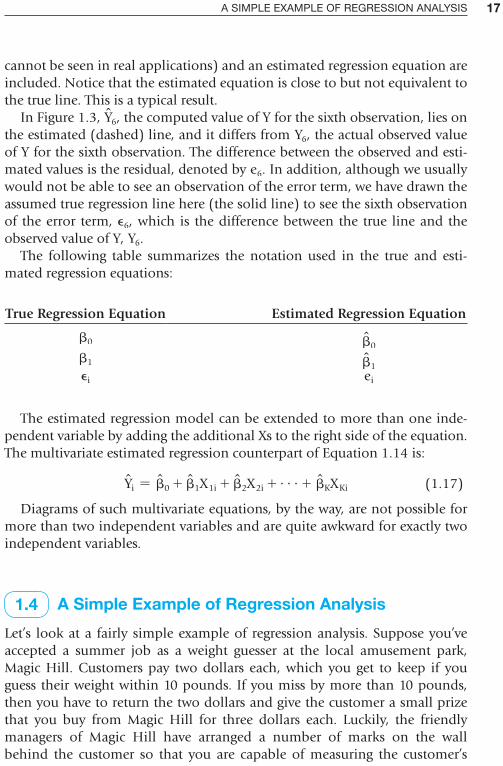
In Figure 1.3, YN6, the computed value of Y for the sixth observation, lies on the estimated (dashed) line, and it differs from Y6, the actual observed value of Y for the sixth observation. The difference between the observed and esti-mated values is the residual, denoted by e6. In addition, although we usually would not be able to see an observation of the error term, we have drawn the assumed true regression line here (the solid line) to see the sixth observation of the error term, e6, which is the difference between the true line and the observed value of Y, Y6.
The following table summarizes the notation used in the true and esti-mated regression equations:
True Regression Equation Estimated Regression Equation
β0 βN 0
β1 βN 1ei ei
The estimated regression model can be extended to more than one inde-pendent variable by adding the additional Xs to the right side of the equation. The multivariate estimated regression counterpart of Equation 1.14 is:
YN i = βN 0 + βN 1X1i + βN 2X2i + g+ βN KXKi (1.17)
Diagrams of such multivariate equations, by the way, are not possible for more than two independent variables and are quite awkward for exactly two independent variables.
1.4 A Simple Example of Regression Analysis
Let’s look at a fairly simple example of regression analysis. Suppose you’ve accepted a summer job as a weight guesser at the local amusement park, Magic Hill. Customers pay two dollars each, which you get to keep if you guess their weight within 10 pounds. If you miss by more than 10 pounds, then you have to return the two dollars and give the customer a small prize that you buy from Magic Hill for three dollars each. Luckily, the friendly managers of Magic Hill have arranged a number of marks on the wall behind the customer so that you are capable of measuring the customer’s
M01_STUD2742_07_SE_C01.indd 17 1/4/16 4:55 PM

18 CHAPTER 1 An Overview Of regressiOn AnAlysis
height accurately. Unfortunately, there is a five-foot wall between you and the customer, so you can tell little about the person except for height and (usually) gender.
On your first day on the job, you do so poorly that you work all day and somehow manage to lose two dollars, so on the second day you decide to collect data to run a regression to estimate the relationship between weight and height. Since most of the participants are male, you decide to limit your sample to males. You hypothesize the following theoretical relationship:
+ Yi = β0 + β1Xi + ei (1.18)
where: Yi = the weight (in pounds) of the ith customer Xi = the height (in inches above 5 feet) of the ith customer ei = the value of the stochastic error term for the ith customer
In this case, the sign of the theoretical relationship between height and weight is believed to be positive (signified by the positive sign above β1 in the general theoretical equation), but you must quantify that relationship in order to estimate weights when given heights. To do this, you need to collect a data set, and you need to apply regression analysis to the data.
The next day you collect the data summarized in Table 1.1 and run your regression on the Magic Hill computer, obtaining the following estimates:
βN 0 = 103.40 βN 1 = 6.38
This means that the equation
Estimated weight = 103.40 + 6.38 # Height (inches above five feet) (1.19)
is worth trying as an alternative to just guessing the weights of your customers. Such an equation estimates weight with a constant base of 103.40 pounds and adds 6.38 pounds for every inch of height over 5 feet. Note that the sign of βN 1 is positive, as you expected.
How well does the equation work? To answer this question, you need to calculate the residuals (Yi minus YN i) from Equation 1.19 to see how many were greater than ten. As can be seen in the last column in Table 1.1, if you had applied the equation to these 20 people, you wouldn’t exactly have got-ten rich, but at least you would have earned $25.00 instead of losing $2.00. Figure 1.4 shows not only Equation 1.19 but also the weight and height data for all 20 customers used as the sample. With a different group of people, the results would of course be different.
Equation 1.19 would probably help a beginning weight guesser, but it could be improved by adding other variables or by collecting a larger sample.
M01_STUD2742_07_SE_C01.indd 18 1/4/16 4:55 PM

19 A simple exAmple Of regressiOn AnAlysis
Such an equation is realistic, though, because it’s likely that every successful weight guesser uses an equation like this without consciously thinking about that concept.
Our goal with this equation was to quantify the theoretical weight/height equation, Equation 1.18, by collecting data (Table 1.1) and calculating an estimated regression, Equation 1.19. Although the true equation, like obser-vations of the stochastic error term, can never be known, we were able to come up with an estimated equation that had the sign we expected for βN 1 and that helped us in our job. Before you decide to quit school or your job and try to make your living guessing weights at Magic Hill, there is quite a bit more to learn about regression analysis, so we’d better move on.
Table 1.1 data for and results of the weight-guessing equation
Observation i
(1)
Height Above 5′ Xi
(2)
Weight Yi (3)
Predicted Weight YNi
(4)
Residual ei (5)
$ Gain or Loss
(6)
1 5.0 140.0 135.3 4.7 +2.00 2 9.0 157.0 160.8 -3.8 +2.00 3 13.0 205.0 186.3 18.7 -3.00 4 12.0 198.0 179.9 18.1 -3.00 5 10.0 162.0 167.2 -5.2 +2.00 6 11.0 174.0 173.6 0.4 +2.00 7 8.0 150.0 154.4 -4.4 +2.00 8 9.0 165.0 160.8 4.2 +2.00 9 10.0 170.0 167.2 2.8 +2.0010 12.0 180.0 179.9 0.1 +2.0011 11.0 170.0 173.6 -3.6 +2.0012 9.0 162.0 160.8 1.2 +2.0013 10.0 165.0 167.2 -2.2 +2.0014 12.0 180.0 179.9 0.1 +2.0015 8.0 160.0 154.4 5.6 +2.0016 9.0 155.0 160.8 -5.8 +2.0017 10.0 165.0 167.2 -2.2 +2.0018 15.0 190.0 199.1 -9.1 +2.0019 13.0 185.0 186.3 -1.3 +2.0020 11.0 155.0 173.6 -18.6 -3.00
tOtAl = $25.00
note: this data set, and every other data set in the text, is available on the text’s website in four formats. datafile = htwt1
M01_STUD2742_07_SE_C01.indd 19 1/4/16 4:55 PM

20 CHAPTER 1 An Overview Of regressiOn AnAlysis
1.5 Using Regression to Explain Housing Prices
As much fun as guessing weights at an amusement park might be, it’s hardly a typical example of the use of regression analysis. For every regression run on such an off-the-wall topic, there are literally hundreds run to describe the reac-tion of GDP to an increase in the money supply, to test an economic theory with new data, or to forecast the effect of a price change on a firm’s sales.
As a more realistic example, let’s look at a model of housing prices. The purchase of a house is probably the most important financial decision in an individual’s life, and one of the key elements in that decision is an appraisal of the house’s value. If you overvalue the house, you can lose thousands of dollars by paying too much; if you undervalue the house, someone might outbid you.
All this wouldn’t be much of a problem if houses were homogeneous products, like corn or gold, that have generally known market prices with which to compare a particular asking price. Such is hardly the case in the real estate market. Consequently, an important element of every housing
Y200
190
180
170
160
150
140
130
120
110
0 1 2 3 4 5 6 7 8Height (over five feet in inches)
Observations
Y-hats
Wei
ght
9 10 11 12 13 14 15 X
Yi = 103.40 + 6.38Xi N
Figure 1.4 A weight-guessing equation
If we plot the data from the weight-guessing example and include the estimated regres-sion line, we can see that the estimated Yns come fairly close to the observed Ys for all but three observations. Find a male friend’s height and weight on the graph. How well does the regression equation work?
M01_STUD2742_07_SE_C01.indd 20 1/4/16 4:55 PM

21 Using regressiOn tO explAin hOUsing prices
purchase is an appraisal of the market value of the house, and many real estate appraisers use regression analysis to help them in their work.
Suppose your family is about to buy a house, but you’re convinced that the owner is asking too much money. The owner says that the asking price of $230,000 is fair because a larger house next door sold for $230,000 about a year ago. You’re not sure it’s reasonable to compare the prices of different-sized houses that were purchased at different times. What can you do to help decide whether to pay the $230,000?
Since you’re taking an econometrics class, you decide to collect data on all local houses that were sold within the last few weeks and to build a regres-sion model of the sales prices of the houses as a function of their sizes.10 Such a data set is called cross-sectional because all of the observations are from the same point in time and represent different individual economic entities (like countries or, in this case, houses) from that same point in time.
To measure the impact of size on price, you include the size of the house as an independent variable in a regression equation that has the price of that house as the dependent variable. You expect a positive sign for the coefficient of size, since big houses cost more to build and tend to be more desirable than small ones. Thus the theoretical model is:
+ PRICEi = β0 + β1SIZEi + ei (1.20)
where: PRICEi = the price (in thousands of $) of the ith house SIZEi = the size (in square feet) of that house ei = the value of the stochastic error term for that house
You collect the records of all recent real estate transactions, find that 43 local houses were sold within the last 4 weeks, and estimate the following regression of those 43 observations:
PRICEi = 40.0 + 0.138SIZEi (1.21)
What do these estimated coefficients mean? The most important coefficient is βN 1 = 0.138, since the reason for the regression is to find out the impact of size on price. This coefficient means that if size increases by 1 square foot,
h
10. It’s unusual for an economist to build a model of price without including some measure of quantity on the right-hand side. Such models of the price of a good as a function of the attributes of that good are called hedonic models and will be discussed in greater depth in Section 11.8. The interested reader is encouraged to skim the first few paragraphs of that section before con-tinuing on with this example.
M01_STUD2742_07_SE_C01.indd 21 1/4/16 4:55 PM
22 CHAPTER 1 An Overview Of regressiOn AnAlysis
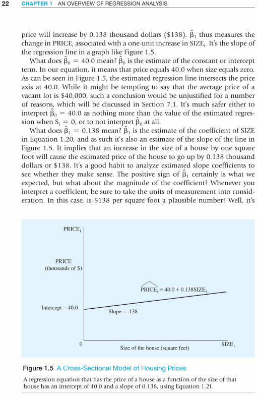
price will increase by 0.138 thousand dollars ($138). βN 1 thus measures the change in PRICEi associated with a one-unit increase in SIZEi. It’s the slope of the regression line in a graph like Figure 1.5.
What does βN 0 = 40.0 mean? βN 0 is the estimate of the constant or intercept term. In our equation, it means that price equals 40.0 when size equals zero. As can be seen in Figure 1.5, the estimated regression line intersects the price axis at 40.0. While it might be tempting to say that the average price of a vacant lot is $40,000, such a conclusion would be unjustified for a number of reasons, which will be discussed in Section 7.1. It’s much safer either to interpret βN 0 = 40.0 as nothing more than the value of the estimated regres-sion when Si = 0, or to not interpret βN 0 at all.
What does βN 1 = 0.138 mean? βN 1 is the estimate of the coefficient of SIZE in Equation 1.20, and as such it’s also an estimate of the slope of the line in Figure 1.5. It implies that an increase in the size of a house by one square foot will cause the estimated price of the house to go up by 0.138 thousand dollars or $138. It’s a good habit to analyze estimated slope coefficients to see whether they make sense. The positive sign of βN 1 certainly is what we expected, but what about the magnitude of the coefficient? Whenever you interpret a coefficient, be sure to take the units of measurement into consid-eration. In this case, is $138 per square foot a plausible number? Well, it’s
PRICEi
0Size of the house (square feet)
Slope = .138Intercept = 40.0
PRICE(thousands of $)
PRICEi = 40.0 + 0.138SIZEi
SIZEi
Figure 1.5 A cross-sectional model of housing prices
A regression equation that has the price of a house as a function of the size of that house has an intercept of 40.0 and a slope of 0.138, using Equation 1.21.
M01_STUD2742_07_SE_C01.indd 22 1/4/16 4:55 PM

23 sUmmAry
hard to know for sure, but it certainly is a lot more reasonable than $1.38 per square foot or $13,800 per square foot!
How can you use this estimated regression to help decide whether to pay $230,000 for the house? If you calculate a YN (predicted price) for a house that is the same size (1,600 square feet) as the one you’re thinking of buying, you can then compare this YN with the asking price of $230,000. To do this, substi-tute 1600 for SIZEi in Equation 1.21, obtaining:
PRICEi = 40.0 + 0.138116002 = 40.0 + 220.8 = 260.8
The house seems to be a good deal. The owner is asking “only” $230,000 for a house when the size implies a price of $260,800! Perhaps your original feeling that the price was too high was a reaction to steep housing prices in general and not a reflection of this specific price.
On the other hand, perhaps the price of a house is influenced by more than just the size of the house. Such multivariate models are the heart of econometrics, and we’ll add more independent variables to Equation 1.21 when we return to this housing price example in Section 11.8.
1.6 Summary
1. Econometrics—literally, “economic measurement”—is a branch of economics that attempts to quantify theoretical relationships. Regres-sion analysis is only one of the techniques used in econometrics, but it is by far the most frequently used.
2. The major uses of econometrics are description, hypothesis testing, and forecasting. The specific econometric techniques employed may vary depending on the use of the research.
3. While regression analysis specifies that a dependent variable is a func-tion of one or more independent variables, regression analysis alone cannot prove or even imply causality.
4. A stochastic error term must be added to all regression equations to account for variations in the dependent variable that are not explained completely by the independent variables. The components of this error term include:a. omitted or left-out variablesb. measurement errors in the datac. an underlying theoretical equation that has a different functional
form (shape) than the regression equationd. purely random and unpredictable events
h
M01_STUD2742_07_SE_C01.indd 23 1/4/16 4:55 PM

24 Chapter 1 An Overview Of regressiOn AnAlysis
ExErcisEs
5. An estimated regression equation is an approximation of the true equation that is obtained by using data from a sample of actual Ys and Xs. Since we can never know the true equation, econometric anal-ysis focuses on this estimated regression equation and the estimates of the regression coefficients. The difference between a particular ob-servation of the dependent variable and the value estimated from the regression equation is called the residual.
(The answers to the even-numbered exercises are in Appendix A.)
1. Write the meaning of each of the following terms without referring to the book (or your notes), and compare your definition with the ver-sion in the text for each:a. constant or intercept (p. 7)b. cross-sectional (p. 21)c. dependent variable (p. 5)d. estimated regression equation (p. 14)e. expected value (p. 9)f. independent (or explanatory) variable (p. 5)g. linear (p. 8)h. multivariate regression model (p. 12)i. regression analysis (p. 5)j. residual (p. 15)k. slope coefficient (p. 7)l. stochastic error term (p. 8)
2. Use your own computer’s regression software and the weight (Y) and height (X) data from Table 1.1 to see if you can reproduce the estimates in Equation 1.19. There are two ways to load the data: You can type in the data yourself or you can download datafile HTWT1 (in Stata, EViews, Excel, or ASCII formats) from the text’s website: http://www.pearsonhighered.com/studenmund. Once the datafile is loaded, run Y = f1X2, and your results should match Equation 1.19. Different programs require different commands to run a regression. For help in how to do this with Stata or EViews, either see the answer to this question in Appendix A or read Appendix 1.7.
M01_STUD2742_07_SE_C01.indd 24 02/02/16 1:48 PM

25exercises
3. Not all regression coefficients have positive expected signs. For example, a Sports Illustrated article by Jaime Diaz reported on a study of golfing putts of various lengths on the Professional Golfers’ Association (PGA) Tour.11 The article included data on the percentage of putts made 1Pi2 as a function of the length of the putt in feet 1Li2. Since the longer the putt, the less likely even a professional is to make it, we’d expect Li to have a negative coefficient in an equation explain-ing Pi. Sure enough, if you estimate an equation on the data in the article, you obtain:
PN i = 83.6 - 4.1Li (1.22)
a. Carefully write out the exact meaning of the coefficient of Li.b. Suppose someone else took the data from the article and estimated:
Pi = 83.6 - 4.1Li + ei
Is this the same result as that of Equation 1.22? If so, what definition do you need to use to convert this equation back to Equation 1.22?
c. Use Equation 1.22 to determine the percent of the time you’d expect a PGA golfer to make a 10-foot putt. Does this seem realistic? How about a 1-foot putt or a 25-foot putt? Do these seem as realistic?
d. Your answer to part c should suggest that there’s a problem in applying a linear regression to these data. What is that problem?
4. Return to the housing price model of Section 1.5 and consider the following equation:
SIZEi = -290 + 3.62 PRICEi (1.23)
where: SIZEi = the size (in square feet) of the ith house PRICEi = the price (in thousands of $) of that house
a. Carefully explain the meaning of each of the estimated regression coefficients.
b. Suppose you’re told that this equation explains a significant por-tion (more than 80 percent) of the variation in the size of a house. Have we shown that high housing prices cause houses to be large? If not, what have we shown?
c. What do you think would happen to the estimated coefficients of this equation if we had measured the price variable in dollars in-stead of in thousands of dollars? Be specific.
h
11. Jaime Diaz, “Perils of Putting,” Sports Illustrated, April 3, 1989, pp. 76–79.
M01_STUD2742_07_SE_C01.indd 25 1/4/16 4:55 PM

26 CHAPTER 1 An Overview Of regressiOn AnAlysis
5. If an equation has more than one independent variable, we have to be careful when we interpret the regression coefficients of that equa-tion. Think, for example, about how you might build an equation to explain the amount of money that different states spend per pupil on public education. The more income a state has, the more they prob-ably spend on public schools, but the faster enrollment is growing, the less there would be to spend on each pupil. Thus, a reasonable equation for per pupil spending would include at least two variables: income and enrollment growth:
Si = β0 + β1Yi + β2Gi + ei (1.24)
where: Si = educational dollars spent per public school student in the ith state
Yi = per capita income in the ith state (in dollars) Gi = the percent growth of public school enrollment in
the ith state
a. State the economic meaning of the coefficients of Y and G. (Hint: Remember to hold the impact of the other variable constant.)
b. If we were to estimate Equation 1.24, what signs would you expect the coefficients of Y and G to have? Why?
c. Silva and Sonstelie estimated a cross-sectional model of per student spending by state that is very similar to Equation 1.24:12
SN i = -183 + 0.1422Yi - 5926Gi (1.25) N = 49
Do these estimated coefficients correspond to your expectations? Explain Equation 1.25 in common sense terms.
d. The authors measured G as a decimal, so if a state had a 10 percent growth in enrollment, then G equaled .10. What would Equation 1.25 have looked like if the authors had measured G in percentage points, so that if a state had 10 percent growth, then G would have equaled 10? (Hint: Write out the actual numbers for the estimated coefficients.)
6. Your friend has an on-campus job making telephone calls to alumni asking for donations to your college’s annual fund, and she wonders
12. Fabio Silva and Jon Sonstelie, “Did Serrano Cause a Decline in School Spending?” National Tax Review, Vol. 48, No. 2, pp. 199–215. The authors also included the tax price for spending per pupil in the ith state as a variable.
M01_STUD2742_07_SE_C01.indd 26 1/4/16 4:55 PM

27exercises
whether her calling is making any difference. In an attempt to mea-sure the impact of student calls on fund raising, she collects data from 50 alums and estimates the following equation:
GIFTi = 2.29 + 0.001INCOMEi + 4.62CALLSi (1.26)
where: GIFTi = the 2016 annual fund donation (in dollars) from the ith alum
INCOMEi = the 2016 estimated income (in dollars) of the ith alum
CALLSi = the # of calls to the ith alum asking for a donation in 2016
a. Carefully explain the meaning of each estimated coefficient. Are the estimated signs what you expected?
b. Why is the left-hand variable in your friend’s equation GIFTi and not GIFTi?
c. Your friend didn’t include the stochastic error term in the estimated equation. Was this a mistake? Why or why not?
d. Suppose that your friend decides to change the units of INCOME from “dollars” to “thousands of dollars.” What will happen to the estimated coefficients of the equation? Be specific.
e. If you could add one more variable to this equation, what would it be? Explain.
7. Let’s return to the wage determination example of Section 1.2. In that example, we built a model of the wage of the ith worker in a particu-lar field as a function of the work experience, education, and gender of that worker:
WAGEi = β0 + β1EXPi + β2EDUi + β3GENDi + ei (1.10)
where: Yi = WAGEi = the wage of the ith worker X1i = EXPi = the years of work experience of the ith worker X2i = EDUi = the years of education beyond high school of the ith worker X3i = GENDi = the gender of the ith worker (1 = male and 0 = female)
a. What is the real-world meaning of β2? (Hint: If you’re unsure where to start, review Section 1.2.)
b. What is the real-world meaning of β3? (Hint: Remember that GEND is a dummy variable.)
h
h
M01_STUD2742_07_SE_C01.indd 27 1/4/16 4:55 PM
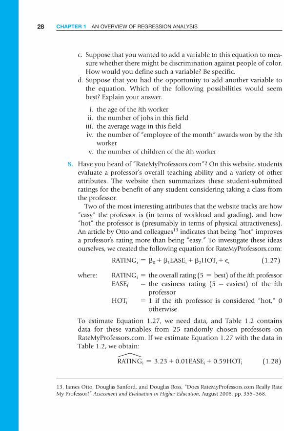
28 CHAPTER 1 An Overview Of regressiOn AnAlysis
c. Suppose that you wanted to add a variable to this equation to mea-sure whether there might be discrimination against people of color. How would you define such a variable? Be specific.
d. Suppose that you had the opportunity to add another variable to the equation. Which of the following possibilities would seem best? Explain your answer.
i. the age of the ith worker ii. the number of jobs in this field iii. the average wage in this field iv. the number of “employee of the month” awards won by the ith
worker v. the number of children of the ith worker
8. Have you heard of “RateMyProfessors.com”? On this website, students evaluate a professor’s overall teaching ability and a variety of other attributes. The website then summarizes these student-submitted ratings for the benefit of any student considering taking a class from the professor.
Two of the most interesting attributes that the website tracks are how “easy” the professor is (in terms of workload and grading), and how “hot” the professor is (presumably in terms of physical attractiveness). An article by Otto and colleagues13 indicates that being “hot” improves a professor’s rating more than being “easy.” To investigate these ideas ourselves, we created the following equation for RateMyProfessors.com:
RATINGi = β0 + β1EASEi + β2HOTi + ei (1.27)
where: RATINGi = the overall rating (5 = best) of the ith professor EASEi = the easiness rating (5 = easiest) of the ith
professor HOTi = 1 if the ith professor is considered “hot,” 0
otherwise
To estimate Equation 1.27, we need data, and Table 1.2 contains data for these variables from 25 randomly chosen professors on RateMyProfessors.com. If we estimate Equation 1.27 with the data in Table 1.2, we obtain:
RATINGi = 3.23 + 0.01EASEi + 0.59HOTi (1.28)
®
13. James Otto, Douglas Sanford, and Douglas Ross, “Does RateMyProfessors.com Really Rate My Professor?” Assessment and Evaluation in Higher Education, August 2008, pp. 355–368.
M01_STUD2742_07_SE_C01.indd 28 1/4/16 4:55 PM
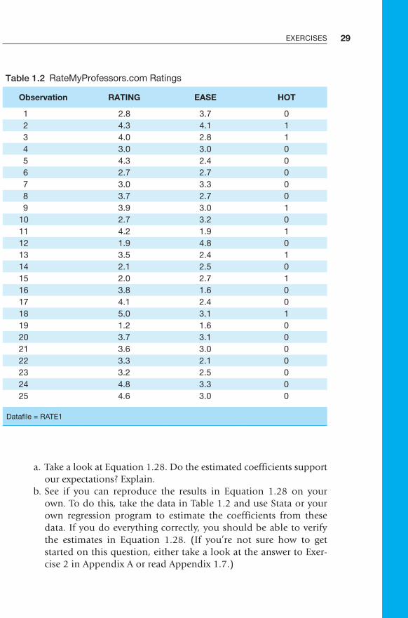
29exercises
a. Take a look at Equation 1.28. Do the estimated coefficients support our expectations? Explain.
b. See if you can reproduce the results in Equation 1.28 on your own. To do this, take the data in Table 1.2 and use Stata or your own regression program to estimate the coefficients from these data. If you do everything correctly, you should be able to verify the estimates in Equation 1.28. (If you’re not sure how to get started on this question, either take a look at the answer to Exer-cise 2 in Appendix A or read Appendix 1.7.)
Table 1.2 ratemyprofessors.com ratings
Observation RATING EASE HOT
1 2.8 3.7 0 2 4.3 4.1 1 3 4.0 2.8 1 4 3.0 3.0 0 5 4.3 2.4 0 6 2.7 2.7 0 7 3.0 3.3 0 8 3.7 2.7 0 9 3.9 3.0 110 2.7 3.2 011 4.2 1.9 112 1.9 4.8 013 3.5 2.4 114 2.1 2.5 015 2.0 2.7 116 3.8 1.6 017 4.1 2.4 018 5.0 3.1 119 1.2 1.6 020 3.7 3.1 021 3.6 3.0 022 3.3 2.1 023 3.2 2.5 024 4.8 3.3 025 4.6 3.0 0
datafile = rAte1
M01_STUD2742_07_SE_C01.indd 29 1/4/16 4:55 PM

30 Chapter 1 An Overview Of regressiOn AnAlysis
c. This model includes two independent variables. Does it make sense to think that the teaching rating of a professor depends on just these two variables? What other variable(s) do you think might be important?
d. Suppose that you were able to add your suggested variable(s) to Equation 1.28. What do you think would happen to the coeffi-cients of EASE and HOT when you added the variable(s)? Would you expect them to change? Would you expect them to remain the same? Explain.
e. (optional) Go to the RateMyProfessors.com website, choose 25 obser-vations at random, and estimate your own version of Equation 1.27. Now compare your regression results to those in Equation 1.28. Do your estimated coefficients have the same signs as those in Equation 1.28? Are your estimated coefficients exactly the same as those in Equation 1.28? Why or why not?
1.7 appendix: Using Stata
Using Econometrics is about, well, using econometrics, and it doesn’t take long to realize that using econometrics requires software. The powerful and user-friendly econometric software package referred to in the text is Stata14, and the purpose of this appendix15 is to give you a brief introduction to Stata.
For most people (including me!), learning new computer software involves some pain. Our goal in this Appendix is to take away as much of that pain as possible. We hope to give you a head start with Stata and also convince you that it’s worth your time to check out the complete “Using Stata” document found online at the Using Econometrics student companion website (http://www.pearsonhighered.com/studenmund). That free docu-ment (yes, free!) is designed to get you up and running in Stata with as little pain as possible. It shows in plain English and clear pictures how to use all the econometric techniques you’ll encounter in the text (and more!)
How do you get Stata? There are a number of ways. Your college or uni-versity may provide Stata access in official computer labs. If it doesn’t (or if you want a personal copy), you can buy and download Stata directly (http://www.stata.com). Fortunately, reasonable student pricing is available.
14. Other econometric software programs that you might encounter include EViews, SAS, R, and SPSS.
15. Written by John Perry, Centre College. Used with permission.
M01_STUD2742_07_SE_C01.indd 30 19/01/16 4:50 PM
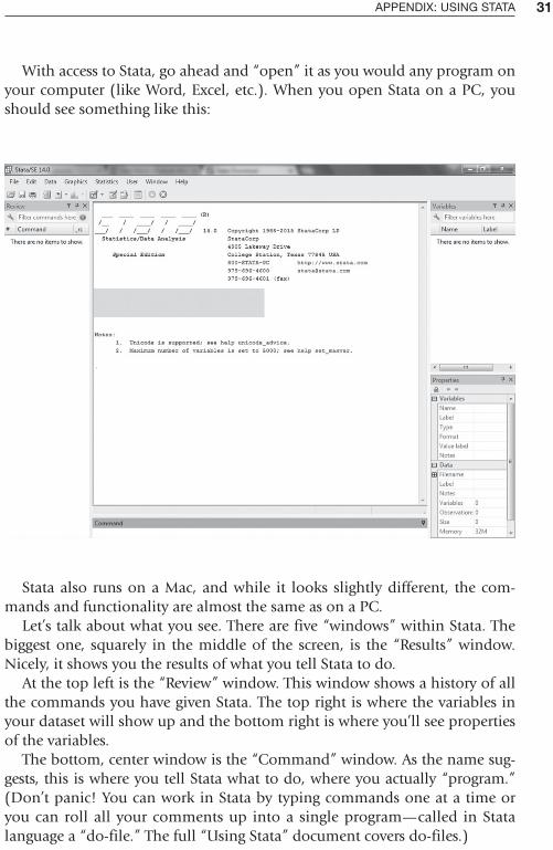
31 Appendix: Using sTATA
With access to Stata, go ahead and “open” it as you would any program on your computer (like Word, Excel, etc.). When you open Stata on a PC, you should see something like this:
Stata also runs on a Mac, and while it looks slightly different, the com-mands and functionality are almost the same as on a PC.
Let’s talk about what you see. There are five “windows” within Stata. The biggest one, squarely in the middle of the screen, is the “Results” window. Nicely, it shows you the results of what you tell Stata to do.
At the top left is the “Review” window. This window shows a history of all the commands you have given Stata. The top right is where the variables in your dataset will show up and the bottom right is where you’ll see properties of the variables.
The bottom, center window is the “Command” window. As the name sug-gests, this is where you tell Stata what to do, where you actually “program.” (Don’t panic! You can work in Stata by typing commands one at a time or you can roll all your comments up into a single program—called in Stata language a “do-file.” The full “Using Stata” document covers do-files.)
M01_STUD2742_07_SE_C01.indd 31 19/01/16 4:50 PM

32 Chapter 1 An Overview Of regressiOn AnAlysis
With Stata open, we should move along and open a dataset. In Section 1.4, you met a dataset from Magic Hill amusement park named HTWT1.dta (“.dta” is the format of a Stata dataset much like “docx” is the format for a Microsoft Word document). It contained the height and weight of 20 people where:
Yi = weight (in pounds) of the ith customerXi = height (in inches above 5 feet) of the ith customer
You can (and should at this point) download and save the dataset to your computer from the student companion website. After doing that, to open the dataset, go to the top left in Stata and click on the folder icon. Next, you’ll be guided to find where you saved HTWT1.dta. Highlight it and click “open.” This is similar to how you’d open a file in any other software (like Word, Excel, etc.). You should see something like this (this time we used Stata on a Mac):
1
2
3
Notice that what you commanded Stata to do—to open HTWT1.dta—is recorded in the Results window (indicated by arrow 1). In Stata, “use” means open. The “use” statement is followed by the pathname (in quotes) where the file is saved on your computer (in my case “/Volumes/ECONOMICS/
M01_STUD2742_07_SE_C01.indd 32 19/01/16 4:50 PM

33 Appendix: Using sTATA
Econometrics/HTWT1.dta”). This command is also recorded in the Review window and indicated by arrow 2.
At the top right, signaled by arrow 3, you see that you have two variables in your Variables window (X and Y). This means you now have data in Stata.
Things are about to get exciting! With our data open in Stata we’re now in a position to replicate Equation 1.19. To do so, type “reg Y X” into the Command window in Stata and hit enter.
The “reg” command, which is short for “regress,” tells Stata to perform a regression. Directly after “reg,” insert the dependent variable (Y in our case). The dependent variable is followed by the model’s independent variables. Equation 1.19 has one independent variable named X. Note that Stata is case sensitive. If you type “y” when the variable’s name is “Y,” Stata will yell.
After giving the “reg Y X” command, you should see something like this:
4
5
6
What you see in the Results window above could easily overwhelm a person. For now, focus on where the three arrows direct. Arrow 4 points to the command that had Stata produce the estimation. Arrow 5 points to the column that lists the variables in the regression: Y, X, and something called “_cons”. That “something” is the model’s intercept term, otherwise known as β0.
M01_STUD2742_07_SE_C01.indd 33 19/01/16 4:50 PM

34 CHAPTER 1 An Overview Of regressiOn AnAlysis
Arrow 6 points to the “Coef.” column, which reports the estimated coef-ficients. The first number in the Coef. column is 6.377093. That is βN 1, the coefficient estimate for X, and matches the 6.38 (rounded) of Equation 1.19. Moving down the Coef. column and next to the _cons is 103.3971. That is βN 0, the estimate of the intercept, which rounds to 103.40.
And with that, you’ve estimated your first regression in Stata! Keep in mind, however, that this short appendix is meant only to help get you started in Stata. The full “Using Stata” document will show you much more—while trying to minimize the pain.
M01_STUD2742_07_SE_C01.indd 34 1/4/16 4:55 PM

35
2.1 Estimating Single-Independent-Variable Models with OLS
2.2 Estimating Multivariate Regression Models with OLS
2.3 Evaluating the Quality of a Regression Equation
2.4 Describing the Overall Fit of the Estimated Model
2.5 An Example of the Misuse of R
2
2.6 Summary and Exercises
2.7 Appendix: Econometric Lab #1
Ordinary Least Squares
The bread and butter of regression analysis is the estimation of the coef-ficients of econometric models using a technique called Ordinary Least Squares (OLS). The first two sections of this chapter summarize the reason-ing behind and the mechanics of OLS. Regression users rely on computers to do the actual OLS calculations, so the emphasis here is on understanding what OLS attempts to do and how it goes about doing it.
How can you tell a good equation from a bad one once it has been esti-mated? There are a number of useful criteria, including the extent to which the estimated equation fits the actual data. A focus on fit is not without per-ils, however, so we share an example of the misuse of this criterion.
The chapter concludes with a new kind of learning tool that we call an econometric lab.
2.1 Estimating Single-Independent-Variable Models with OLS
The purpose of regression analysis is to take a purely theoretical equation like:
Yi = β0 + β1Xi + ei (2.1)
Chapter 2
M02_STUD2742_07_SE_C02.indd 35 1/4/16 6:46 PM

36 ChAptER 2 Ordinary Least squares
and use a set of data to create an estimated equation like:
Yni = βn 0 + βn 1Xi (2.2)
where each “hat” indicates a sample estimate of the true population value. (In the case of Y, the “true population value” is E3Y ƒ X4.) The purpose of the estimation technique is to obtain numerical values for the coefficients of an otherwise completely theoretical regression equation.
The most widely used method of obtaining these estimates is Ordinary Least Squares (OLS), which has become so standard that its estimates are presented as a point of reference even when results from other estimation techniques are used. Ordinary Least Squares (OLS) is a regression estimation technique that calculates the βns so as to minimize the sum of the squared residuals, thus:1
OLS minimizes aNi = 1
e
2i 1i = 1, 2, . . . , N2 (2.3)
Since these residuals (eis) are the differences between the actual Ys and the estimated Ys produced by the regression (the Yns in Equation 2.2), Equation 2.3 is equivalent to saying that OLS minimizes a 1Yi - Yni22.
Why Use Ordinary Least Squares?
Although OLS is the most-used regression estimation technique, it’s not the only one. Indeed, econometricians have developed what seem like zillions of different estimation techniques, a number of which we’ll discuss later in this text.
There are at least three important reasons for using OLS to estimate regression models:
1. OLS is relatively easy to use.
2. The goal of minimizing a e 2i is quite appropriate from a theoretical
point of view.
3. OLS estimates have a number of useful characteristics.
1. The summation symbol, a , indicates that all terms to its right should be added (or summed) over the range of the i values attached to the bottom and top of the symbol. In Equation 2.3, for example, this would mean adding up e2
i for all integer values between 1 and N:
aNi = 1
e2i = e2
1 + e22 + g + e2
N
Often the a notation is simply written as a
i, and it is assumed that the summation is over all
observations from i = 1 to i = N. Sometimes, the i is omitted entirely and the same assump-tion is made implicitly.
M02_STUD2742_07_SE_C02.indd 36 1/4/16 6:46 PM

37 estimating singLe-independent-VariabLe mOdeLs with OLs
The first reason for using OLS is that it’s the simplest of all econometric estimation techniques. Most other techniques involve complicated nonlin-ear formulas or iterative procedures, many of which are extensions of OLS itself. In contrast, OLS estimates are simple enough that, if you had to, you could calculate them without using a computer or a calculator (for a single-independent-variable model). Indeed, in the “dark ages” before computers and calculators, econometricians calculated OLS estimates by hand!
The second reason for using OLS is that minimizing the summed, squared residuals is a reasonable goal for an estimation technique. To see this, recall that the residual measures how close the estimated regression equation comes to the actual observed data:
ei = Yi - Yni 1i = 1, 2, . . ., N2 (1.15)
Since it’s reasonable to want our estimated regression equation to be as close as possible to the observed data, you might think that you’d want to mini-mize these residuals. The main problem with simply totaling the residuals is that ei can be negative as well as positive. Thus, negative and positive residu-als might cancel each other out, allowing a wildly inaccurate equation to have a very low a ei. For example, if Y = 100,000 for two consecutive obser-vations and if your equation predicts 1.1 million and -900,000, respectively, your residuals will be +1 million and -1 million, which add up to zero!
We could get around this problem by minimizing the sum of the abso-lute values of the residuals, but absolute values are difficult to work with mathematically. Luckily, minimizing the summed squared residuals does the job. Squared functions pose no unusual mathematical difficulties in terms of manipulations, and the technique avoids canceling positive and negative residuals because squared terms are always positive.
The final reason for using OLS is that its estimates have at least two useful properties:2
1. The sum of the residuals is exactly zero.
2. OLS can be shown to be the “best” estimator possible under a set of specific assumptions. We’ll define “best” in Chapter 4.
An estimator is a mathematical technique that is applied to a sample of data to produce a real-world numerical estimate of the true population regression coefficient (or other parameters). Thus, OLS is an estimator, and a βn produced by OLS is an estimate.
2. These properties, and indeed all the properties of OLS that we discuss in this book, are true as long as a constant term is included in the regression equation. For more on this, see Section 7.1.
M02_STUD2742_07_SE_C02.indd 37 1/4/16 6:46 PM

38 ChAptER 2 Ordinary Least squares
how Does OLS Work?
How would OLS estimate a single-independent-variable regression model like Equation 2.1?
Yi = β0 + β1Xi + ei (2.1)
OLS selects those estimates of β0 and β1 that minimize the squared residuals, summed over all the sample data points.
For an equation with just one independent variable, these coefficients are:3
βn 1 =aNi = 1
31Xi - X2 1Yi - Y24
aNi = 1
1Xi - X22
(2.4)
and, given this estimate of β1,
βn0 = Y - βn 1X (2.5)
where X = the mean of X, or aXi/N, and Y = the mean of Y, or aYi/N. Note that for each different data set, we’ll get different estimates of β1 and β0, depending on the sample.
3. Since
aNi = 1
e2i = aN
i = 1 1Yi - Yni22
and Yni = βn0 + βnX1i, OLS actually minimizes
ai
e2i = a
i 1Yi - βn0 - βn1Xi22
by choosing the βns that do so. For those with a moderate grasp of calculus and algebra, the derivation of these equations is informative.
M02_STUD2742_07_SE_C02.indd 38 1/4/16 6:46 PM

39 estimating singLe-independent-VariabLe mOdeLs with OLs
An Illustration of OLS Estimation
The equations for calculating regression coefficients might seem a little for-bidding, but it’s not hard to apply them yourself to data sets that have only a few observations and independent variables. Although you’ll usually want to use regression software packages to do your estimation, you’ll understand OLS better if you work through the following illustration.
To keep things simple, let’s attempt to estimate the regression coefficients of the height and weight data given in Section 1.4. For your convenience in following this illustration, the original data are reproduced in Table 2.1. As was noted previously, the formulas for OLS estimation for a regression equa-tion with one independent variable are Equations 2.4 and 2.5:
βn 1 =aNi = 1
31Xi - X2 1Yi - Y24
aNi = 1
1Xi - X22
(2.4)
βn 0 = Y - βn 1X (2.5)
If we undertake the calculations outlined in Table 2.1 and substitute them into Equations 2.4 and 2.5, we obtain these values:
βn 1 =590.2092.50
= 6.38
βn0 = 169.4 - 16.38 # 10.352 = 103.4
or
Yni = 103.4 + 6.38Xi (2.6)
If you compare these estimates, you’ll find that the manually calculated coef-ficient estimates are the same as the computer regression results summarized in Section 1.4.
As can be seen in Table 2.1, the sum of the Yns (column 8) equals the sum of the Ys (column 2), so the sum of the residuals (column 9) does indeed equal zero (except for rounding errors).
M02_STUD2742_07_SE_C02.indd 39 1/4/16 6:46 PM

40 ChAptER 2 Ordinary Least squares
2.2 Estimating Multivariate Regression Models with OLS
Let’s face it: only a few dependent variables can be explained fully by a single independent variable. A person’s weight, for example, is influenced by more than just that person’s height. What about bone structure, percent body fat, exercise habits, or diet?
As important as additional explanatory variables might seem to the height/weight example, there’s even more reason to include a variety of inde-pendent variables in economic and business applications. Although the per capita quantity consumed of a product is certainly affected by price, that’s not
Table 2.1 the Calculation of estimated regression Coefficients for the weight/height example
Raw Data Required Intermediate Calculations
i (1)
Yi (2)
Xi (3)
1Yi − Y 2 (4)
1Xi − X 2 (5)
1Xi − X 22 (6)
1Xi − X 2 1Yi − Y 2 (7)
Yni (8)
ei = Yi − Yni (9)
1 140 5 -29.40 -5.35 28.62 157.29 135.3 4.7 2 157 9 -12.40 -1.35 1.82 16.74 160.8 -3.8 3 205 13 35.60 2.65 7.02 94.34 186.3 18.7 4 198 12 28.60 1.65 2.72 47.19 179.9 18.1 5 162 10 -7.40 -0.35 0.12 2.59 167.2 -5.2 6 174 11 4.60 0.65 0.42 2.99 173.5 0.5 7 150 8 -19.40 -2.35 5.52 45.59 154.4 -4.4 8 165 9 -4.40 -1.35 1.82 5.94 160.8 4.2 9 170 10 0.60 -0.35 0.12 -0.21 167.2 2.810 180 12 10.60 1.65 2.72 17.49 179.9 0.111 170 11 0.60 0.65 0.42 0.39 173.5 -3.512 162 9 -7.40 -1.35 1.82 9.99 160.8 1.213 165 10 -4.40 -0.35 0.12 1.54 167.2 -2.214 180 12 10.60 1.65 2.72 17.49 179.9 0.115 160 8 -9.40 -2.35 5.52 22.09 154.4 5.616 155 9 -14.40 -1.35 1.82 19.44 160.8 -5.817 165 10 -4.40 -0.35 0.12 1.54 167.2 -2.218 190 15 20.60 4.65 21.62 95.79 199.1 -9.119 185 13 15.60 2.65 7.02 41.34 186.3 -1.320 155 11 -14.40 0.65 0.42 -9.36 173.5 -18.5
sum 3388 207 0.0 0.0 92.50 590.20 3388.0 -0.0mean 169.4 10.35 0.0 0.0 169.4 0.0
M02_STUD2742_07_SE_C02.indd 40 1/4/16 6:46 PM

41 estimating muLtiVariate regressiOn mOdeLs with OLs
the whole story. Advertising, per capita income, the prices of substitutes, the influence of foreign markets, the quality of customer service, possible fads, and changing tastes all are important in real-world models. As a result, it’s vital to move from single-independent-variable regressions to multivariate regression models, or equations with more than one independent variable.
the Meaning of Multivariate Regression Coefficients
The general multivariate regression model with K independent variables can be represented by Equation 1.11:
Yi = β0 + β1X1i + β2X2i + g + βKXKi + ei (1.11)
where i, as before, goes from 1 to N and indicates the observation number. Thus, X1i indicates the ith observation of independent variable X1, while X2i indicates the ith observation of another independent variable, X2.
The biggest difference between a single-independent-variable regression model and a multivariate regression model is in the interpretation of the latter’s slope coefficients. These coefficients, often called partial regression coefficients, are defined to allow a researcher to distinguish the impact of one variable from that of other independent variables.
Specifically, a multivariate regression coefficient indicates the change in the dependent variable associated with a one-unit increase in the independent variable in question, holding constant the other independent variables in the equation.
This last italicized phrase is a key to understanding multiple regression (as multivariate regression is often called). The coefficient β1 measures the impact on Y of a one-unit increase in X1, holding constant X2, X3, . . . and XK but not holding constant any relevant variables that might have been omitted from the equation (e.g., XK + 1). The coefficient β0 is the value of Y when all the Xs and the error term equal zero. As you’ll learn in Section 7.1, you should always include a constant term in a regression equation, but you should not rely on estimates of β0 for inference.
As an example, let’s consider the following annual model of the per capita consumption of beef in the United States:
CBt = 37.54 - 0.88Pt + 11.9Ydt (2.7)
9
M02_STUD2742_07_SE_C02.indd 41 1/4/16 6:46 PM

42 ChAptER 2 Ordinary Least squares
where: CBt = the per capita consumption of beef in year t (in pounds per person)
Pt = the price of beef in year t (in cents per pound)Ydt = the per capita disposable income in year t (in thousands of
dollars)
The estimated coefficient of income, 11.9, tells us that beef consumption will increase by 11.9 pounds per person if per capita disposable income goes up by $1,000, holding constant the price of beef. The ability to hold price con-stant is crucial because we’d expect such a large increase in per capita income to stimulate demand, therefore pushing up prices and making it hard to dis-tinguish the effect of the income increase from the effect of the price increase. The multivariate regression estimate allows us to focus on the impact of the income variable by holding the price variable constant. Note, however, that the equation does not hold constant other possible variables (like the price of a substitute) because these variables are not included in Equation 2.7.
Before we move on to the next section, let’s take the time to analyze the estimated coefficients of Equation 2.7 in a bit more depth. First, the coef-ficient of P tells us the impact of a one-cent increase in the price of beef on the per capita consumption of beef, holding constant per capita income. Do you agree that the estimated coefficient has the sign that economic theory would predict? Second, think about how the estimated coefficients would change if we were to change the units of disposable income from “thousands of dollars” to “dollars.” The estimated equation would remain the same except that the coefficient of Yd would decrease from 11.9 to 0.0119.
OLS Estimation of Multivariate Regression Models
The application of OLS to an equation with more than one independent variable is quite similar to its application to a single-independent-variable model. To see this, consider the estimation of the simplest possible multivari-ate model, one with just two independent variables:
Yi = β0 + β1X1i + β2X2i + ei (2.8)
The goal of OLS is to choose those βns that minimize the summed squared residuals. These residuals are now from a multivariate model, but they can be minimized using the same mathematical approach used in Section 2.1. Thus the OLS estimation of multivariate models is identical in general approach to the OLS estimation of models with just one independent variable. The
M02_STUD2742_07_SE_C02.indd 42 1/4/16 6:46 PM

43 estimating muLtiVariate regressiOn mOdeLs with OLs
equations themselves are more cumbersome,4 but the underlying principle of estimating βns that minimize the summed squared residuals remains the same.
Luckily, user-friendly computer packages can calculate estimates with these unwieldy equations in less than a second of computer time. Indeed, only some-one lost in time or stranded on a desert island would bother estimating a multi-variate regression model without a computer. The rest of us will use Stata, EViews, SPSS, SAS, or any of the other commercially available regression packages.
An Example of a Multivariate Regression Model
As an example of multivariate regression, let’s take a look at a model of financial aid awards at a liberal arts college. The dependent variable in such a study would be the amount, in dollars, awarded to a particular financial aid applicant:
FINAIDi = the financial aid (measured in dollars of grant per year) awarded to the ith applicant
What kinds of independent variables might influence the amount of finan-cial aid received by a given student? Well, most aid is either need-based or merit-based, so it makes sense to consider a model that includes at least these two attributes:
FINAIDi = β0 + β-
1PARENTi + β+
2HSRANKi + ei (2.9)
where: PARENTi = the amount (in dollars per year) that the parents of the ith student are judged able to contribute to college expenses
HSRANKi = the ith student’s GPA rank in high school, measured as a percentage (ranging from a low of 0 to a high of 100)
4. For Equation 2.8, the estimated coefficients are:
βn1 =1a yx121a x2
22 - 1a yx221a x1x221a x2
121a x222 - 1a x1x222
βn2 =1a yx221a x2
12 - 1a yx121a x1x221a x2
121a x222 - 1a x1x222
βn0 = Y - βn1X1 - βn2X2
where lowercase variables indicate deviations from the mean, as in y = Yi - Y; x1 = X1i - X1; and x2 = X2i - X2.
M02_STUD2742_07_SE_C02.indd 43 1/4/16 6:46 PM
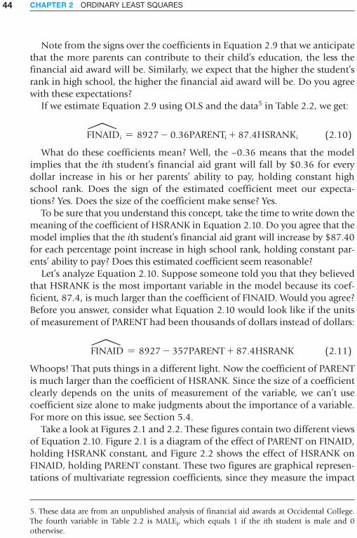
44 ChAptER 2 Ordinary Least squares
Note from the signs over the coefficients in Equation 2.9 that we anticipate that the more parents can contribute to their child’s education, the less the financial aid award will be. Similarly, we expect that the higher the student’s rank in high school, the higher the financial aid award will be. Do you agree with these expectations?
If we estimate Equation 2.9 using OLS and the data5 in Table 2.2, we get:
FINAIDi = 8927 - 0.36PARENTi + 87.4HSRANKi (2.10)
What do these coefficients mean? Well, the –0.36 means that the model implies that the ith student’s financial aid grant will fall by $0.36 for every dollar increase in his or her parents’ ability to pay, holding constant high school rank. Does the sign of the estimated coefficient meet our expecta-tions? Yes. Does the size of the coefficient make sense? Yes.
To be sure that you understand this concept, take the time to write down the meaning of the coefficient of HSRANK in Equation 2.10. Do you agree that the model implies that the ith student’s financial aid grant will increase by $87.40 for each percentage point increase in high school rank, holding constant par-ents’ ability to pay? Does this estimated coefficient seem reasonable?
Let’s analyze Equation 2.10. Suppose someone told you that they believed that HSRANK is the most important variable in the model because its coef-ficient, 87.4, is much larger than the coefficient of FINAID. Would you agree? Before you answer, consider what Equation 2.10 would look like if the units of measurement of PARENT had been thousands of dollars instead of dollars:
FINAID = 8927 - 357PARENT + 87.4HSRANK (2.11)
Whoops! That puts things in a different light. Now the coefficient of PARENT is much larger than the coefficient of HSRANK. Since the size of a coefficient clearly depends on the units of measurement of the variable, we can’t use coefficient size alone to make judgments about the importance of a variable. For more on this issue, see Section 5.4.
Take a look at Figures 2.1 and 2.2. These figures contain two different views of Equation 2.10. Figure 2.1 is a diagram of the effect of PARENT on FINAID, holding HSRANK constant, and Figure 2.2 shows the effect of HSRANK on FINAID, holding PARENT constant. These two figures are graphical represen-tations of multivariate regression coefficients, since they measure the impact
ii
5. These data are from an unpublished analysis of financial aid awards at Occidental College. The fourth variable in Table 2.2 is MALEi, which equals 1 if the ith student is male and 0 otherwise.
M02_STUD2742_07_SE_C02.indd 44 1/4/16 6:46 PM

45 estimating muLtiVariate regressiOn mOdeLs with OLs
0 PARENTi
FINAIDi
Slope = -0.36 = d1 (holding HSRANKi constant)N
Figure 2.1 Financial aid as a Function of parents’ ability to pay
In Equation 2.10, an increase of one dollar in the parents’ ability to pay decreases the financial aid award by $0.36, holding constant high school rank.
0 HSRANKi
FINAIDi
Slope = 87.40 = d2 (holding PARENTi constant)N
Figure 2.2 Financial aid as a Function of high school rank
In Equation 2.10, an increase of one percentage point in high school rank increases the financial aid award by $87.40, holding constant parents’ ability to pay.
M02_STUD2742_07_SE_C02.indd 45 1/4/16 6:46 PM

46 ChAptER 2 Ordinary Least squares
Table 2.2 data for the Financial aid example
i FINAID pARENt hSRANK MALE 1 19,640 0 92 0 2 8,325 9,147 44 1 3 12,950 7,063 89 0 4 700 33,344 97 1 5 7,000 20,497 95 1 6 11,325 10,487 96 0 7 19,165 519 98 1 8 7,000 31,758 70 0 9 7,925 16,358 49 010 11,475 10,495 80 011 18,790 0 90 012 8,890 18,304 75 113 17,590 2,059 91 114 17,765 0 81 015 14,100 15,602 98 016 18,965 0 80 017 4,500 22,259 90 118 7,950 5,014 82 119 7,000 34,266 98 120 7,275 11,569 50 021 8,000 30,260 98 122 4,290 19,617 40 123 8,175 12,934 49 124 11,350 8,349 91 025 15,325 5,392 82 126 22,148 0 98 027 17,420 3,207 99 028 18,990 0 90 029 11,175 10,894 97 030 14,100 5,010 59 031 7,000 24,718 97 132 7,850 9,715 84 133 0 64,305 84 034 7,000 31,947 98 135 16,100 8,683 95 136 8,000 24,817 99 037 8,500 8,720 20 138 7,575 12,750 89 139 13,750 2,417 41 140 7,000 26,846 92 141 11,200 7,013 86 142 14,450 6,300 87 0
M02_STUD2742_07_SE_C02.indd 46 1/4/16 6:46 PM

47 estimating muLtiVariate regressiOn mOdeLs with OLs
on the dependent variable of a given independent variable, holding constant the other variables in the equation.
total, Explained, and Residual Sums of Squares
Before going on, let’s pause to develop some measures of how much of the variation of the dependent variable is explained by the estimated regression equation. Such comparison of the estimated values with the actual values can help a researcher judge the adequacy of an estimated regression.
Econometricians use the squared variations of Y around its mean as a measure of the amount of variation to be explained by the regression. This computed quantity is usually called the total sum of squares, or TSS, and is written as:
TSS = aNi = 1
1Yi - Y22 (2.12)
For Ordinary Least Squares, the total sum of squares has two components, variation that can be explained by the regression and variation that cannot:
ai
1Yi - Y22 = ai
1Yni - Y22 + ai
e2i (2.13)
Total Sum = Explained + Residual of Sum of Sum of Squares Squares Squares (TSS) (ESS) (RSS)
This is usually called the decomposition of variance.
i FINAID pARENt hSRANK MALE43 15,265 3,909 84 044 20,470 2,027 99 145 9,550 12,592 89 046 15,970 0 57 047 12,190 6,249 84 048 11,800 6,237 81 049 21,640 0 99 050 9,200 10,535 68 0
datafile = Finaid2
Table 2.2 (continued)
M02_STUD2742_07_SE_C02.indd 47 1/4/16 6:46 PM
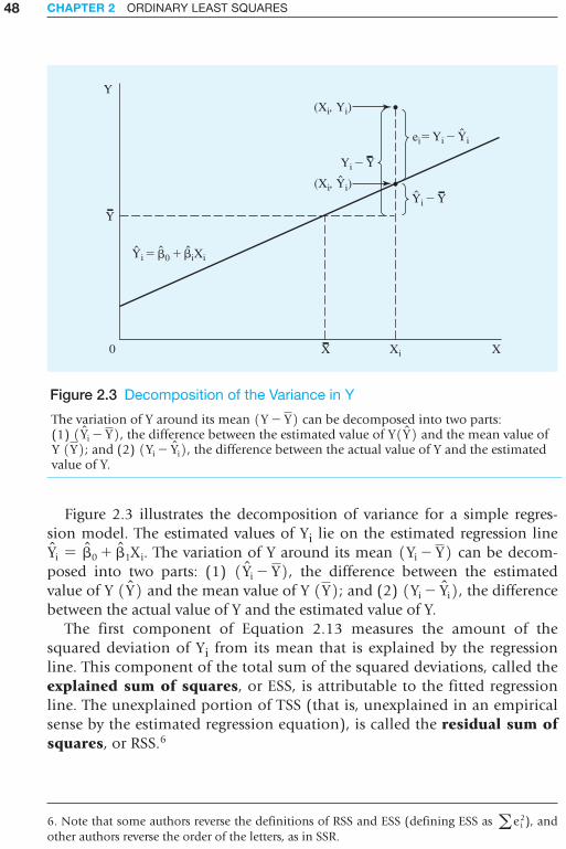
48 ChAptER 2 Ordinary Least squares
Figure 2.3 illustrates the decomposition of variance for a simple regres-sion model. The estimated values of Yi lie on the estimated regression line Yni = βn 0 + βn 1Xi. The variation of Y around its mean 1Yi - Y2 can be decom-posed into two parts: (1) 1Yni - Y2, the difference between the estimated value of Y 1Yn 2 and the mean value of Y 1Y2; and (2) 1Yi - Yni2, the difference between the actual value of Y and the estimated value of Y.
The first component of Equation 2.13 measures the amount of the squared deviation of Yi from its mean that is explained by the regression line. This component of the total sum of the squared deviations, called the explained sum of squares, or ESS, is attributable to the fitted regression line. The unexplained portion of TSS (that is, unexplained in an empirical sense by the estimated regression equation), is called the residual sum of squares, or RSS.6
Y
0 XiX
= Yi - Yi
Yi - Y
X
d0
ei
Y
(Xi, Yi)
(Xi, Yi)
Yi - Y
Yi = + diXiN N N
N
N
N
Figure 2.3 decomposition of the Variance in y
The variation of Y around its mean 1Y - Y2 can be decomposed into two parts: (1) 1Yni - Y2, the difference between the estimated value of Y1Yn 2 and the mean value of Y 1Y2; and (2) 1Yi - Yni2, the difference between the actual value of Y and the estimated value of Y.
6. Note that some authors reverse the definitions of RSS and ESS (defining ESS as a e
2i ), and
other authors reverse the order of the letters, as in SSR.
M02_STUD2742_07_SE_C02.indd 48 1/4/16 6:46 PM

49 eVaLuating the quaLity OF a regressiOn equatiOn
We can see from Equation 2.13 that the smaller the RSS is relative to the TSS, the better the estimated regression line fits the data. OLS is the estimat-ing technique that minimizes the RSS and therefore maximizes the ESS for a given TSS.
2.3 Evaluating the Quality of a Regression Equation
If the bread and butter of regression analysis is OLS estimation, then the heart and soul of econometrics is figuring out how good these OLS estimates are.
Many beginning econometricians have a tendency to accept regression estimates as they come out of a computer, or as they are published in an arti-cle, without thinking about the meaning or validity of those estimates. Such blind faith makes as much sense as buying an entire wardrobe of clothes without trying them on. Some of the clothes will fit just fine, but many others will turn out to be big (or small) mistakes.
Instead, the job of an econometrician is to carefully think about and eval-uate every aspect of the equation, from the underlying theory to the quality of the data, before accepting a regression result as valid. In fact, most good econometricians spend quite a bit of time thinking about what to expect from an equation before they estimate that equation.
Once the computer estimates have been produced, however, it’s time to evaluate the regression results. The list of questions that should be asked dur-ing such an evaluation is long. For example:
1. Is the equation supported by sound theory?
2. How well does the estimated regression fit the data?
3. Is the data set reasonably large and accurate?
4. Is OLS the best estimator to be used for this equation?
5. How well do the estimated coefficients correspond to the expectations developed by the researcher before the data were collected?
6. Are all the obviously important variables included in the equation?
7. Has the most theoretically logical functional form been used?
8. Does the regression appear to be free of major econometric problems?
The goal of this text is to help you develop the ability to ask and appropri-ately answer these kinds of questions. In fact, the number in front of each question above roughly corresponds to the chapter in which we’ll address the issues raised by that question. Since this is Chapter 2, it’ll come as no surprise
M02_STUD2742_07_SE_C02.indd 49 1/4/16 6:46 PM
50 ChAptER 2 Ordinary Least squares
to you to hear that the rest of the chapter will be devoted to the second of these topics—the overall fit of the estimated model.
2.4 Describing the Overall Fit of the Estimated Model
Let’s face it: we expect that a good estimated regression equation will explain the variation of the dependent variable in the sample fairly accurately. If it does, we say that the estimated model fits the data well.
Looking at the overall fit of an estimated model is useful not only for evaluating the quality of the regression, but also for comparing models that have different data sets or combinations of independent variables. We can never be sure that one estimated model represents the truth any more than another, but evaluating the quality of the fit of the equation is one ingredient in a choice between different formulations of a regression model. Be careful, however! The quality of the fit is a minor ingredient in this choice, and many beginning researchers allow themselves to be overly influenced by it.
R2
The simplest commonly used measure of fit is R2, or the coefficient of deter-mination. R2 is the ratio of the explained sum of squares to the total sum of squares:
R2 =ESSTSS
= 1 -RSSTSS
= 1 - a e
2i
a 1Yi - Y22 (2.14)
The higher R2 is, the closer the estimated regression equation fits the sample data. Measures of this type are called “goodness of fit” measures. R2 measures the percentage of the variation of Y around Y that is explained by the regres-sion equation. Since OLS selects the coefficient estimates that minimize RSS, OLS provides the largest possible R2, given a linear model. Since TSS, RSS, and ESS are all nonnegative (being squared deviations), and since ESS … TSS, then R2 must lie in the interval 0 … R2 … 1. A value of R2 close to one shows an excellent overall fit, whereas a value near zero shows a failure of the esti-mated regression equation to explain the values of Yi better than could be explained by the sample mean Y.
Figures 2.4 through 2.6 demonstrate some extremes. Figure 2.4 shows an X and Y that are unrelated. The fitted regression line might as well be Yn = Y, the same value it would have if X were omitted. As a result, the estimated
M02_STUD2742_07_SE_C02.indd 50 1/4/16 6:46 PM
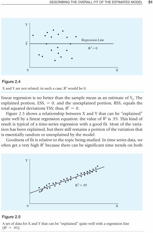
51 desCribing the OVeraLL Fit OF the estimated mOdeL
linear regression is no better than the sample mean as an estimate of Yi. The explained portion, ESS, = 0, and the unexplained portion, RSS, equals the total squared deviations TSS; thus, R2 = 0.
Figure 2.5 shows a relationship between X and Y that can be “explained” quite well by a linear regression equation: the value of R2 is .95. This kind of result is typical of a time-series regression with a good fit. Most of the varia-tion has been explained, but there still remains a portion of the variation that is essentially random or unexplained by the model.
Goodness of fit is relative to the topic being studied. In time series data, we often get a very high R2 because there can be significant time trends on both
Y
Y
0 X
Regression Line
R2 = 0
Figure 2.4
X and Y are not related; in such a case, R2 would be 0.
Y
0 X
R2 = .95
Figure 2.5
A set of data for X and Y that can be “explained” quite well with a regression line (R2 = .95).
M02_STUD2742_07_SE_C02.indd 51 1/4/16 6:46 PM

52 ChAptER 2 Ordinary Least squares
sides of the equation. In cross-sectional data, we often get low R2s because the observations (say, countries) differ in ways that are not easily quantified. In such a situation, an R2 of .50 might be considered a good fit, and research-ers would tend to focus on identifying the variables that have a substantive impact on the dependent variable, not on R2. In other words, there is no sim-ple method of determining how high R2 must be for the fit to be considered satisfactory. Instead, knowing when R2 is relatively large or small is a matter of experience. It should be noted that a high R2 does not imply that changes in X lead to changes in Y, as there may be an underlying variable whose changes lead to changes in both X and Y simultaneously.
Figure 2.6 shows a perfect fit of R2 = 1. Such a fit implies that no estima-tion is required. The relationship is completely deterministic, and the slope and intercept can be calculated from the coordinates of any two points. In fact, reported equations with R2s equal to (or very near) one should be viewed with suspicion; they very likely do not explain the movements of the dependent variable Y in terms of the causal proposition advanced, even though they explain them empirically. This caution applies to economic applications, but not necessarily to those in fields like physics or chemistry.
R
2, the Adjusted R2
A major problem with R2 is that adding another independent variable to a particular equation can never decrease R2. That is, if you compare two equa-tions that are identical (same dependent variable and independent vari-ables), except that one has an additional independent variable, the equation
Y
0 X
R2 = 1
Figure 2.6
A perfect fit: all the data points are on the regression line, and the resulting R2 is 1.
M02_STUD2742_07_SE_C02.indd 52 1/4/16 6:46 PM

53 desCribing the OVeraLL Fit OF the estimated mOdeL
with the greater number of independent variables will always have a better (or equal) fit as measured by R2.
To see this, recall the equation for R2, Equation 2.14.
R2 =ESSTSS
= 1 -RSSTSS
= 1 - a e
2i
a 1Yi - Y22 (2.14)
What will happen to R2 if we add a variable to the equation? Adding a vari-able can’t change TSS (can you figure out why?), but in most cases the added variable will reduce RSS, so R2 will rise. You know that RSS will never increase because the OLS program could always set the coefficient of the added vari-able equal to zero, thus giving the same fit as the previous equation. The coefficient of the newly added variable being zero is the only circumstance in which R2 will stay the same when a variable is added. Otherwise, R2 will always increase when a variable is added to an equation.
Perhaps an example will make this clear. Let’s return to our weight guess-ing regression, Equation 1.19:
Estimated weight = 103.40 + 6.38 Height 1over five feet2The R2 for this equation is .74. If we now add a completely nonsensical
variable to the equation (say, the campus post office box number of each individual in question), then it turns out that the results become:
Estimated weight = 102.35 + 6.36 1Height 7 five feet2 + 0.02 1Box#2but the R2 for this equation is .75! Thus, an individual using R2 alone as the measure of the quality of the fit of the regression would choose the second version as better fitting.
The inclusion of the campus post office box variable not only adds a nonsensical variable to the equation, but it also requires the estimation of another coefficient. This lessens the degrees of freedom, or the excess of the number of observations (N) over the number of coefficients (including the intercept) estimated (K + 1). For instance, when the campus box number variable is added to the weight/height example, the number of observations stays constant at 20, but the number of estimated coefficients increases from 2 to 3, so the number of degrees of freedom falls from 18 to 17. This decrease has a cost, since the lower the degrees of freedom, the less reliable the esti-mates are likely to be. Thus, the increase in the quality of the fit caused by the addition of a variable needs to be compared to the decrease in the degrees of freedom before a decision can be made with respect to the statistical impact of the added variable.
To sum, R2 is of little help if we’re trying to decide whether adding a variable to an equation improves our ability to meaningfully explain the
M02_STUD2742_07_SE_C02.indd 53 1/4/16 6:46 PM

54 ChAptER 2 Ordinary Least squares
dependent variable. Because of this problem, econometricians have developed another measure of the quality of the fit of an equation. That measure is R
2 (pronounced R-bar-squared), which is R2 adjusted for degrees of freedom:
R
2 = 1 - a e
2i /1N - K - 12
a 1Yi - Y22/1N - 12 (2.15)
R
2 measures the percentage of the variation of Y around its mean that is explained by the regression equation, adjusted for degrees of freedom.
R
2 can be used to compare the fits of equations with the same depen-dent variable and different numbers of independent variables. Because of this property, most researchers automatically use R
2 instead of R2 when evaluating the fit of their estimated regression equations. Note, how-ever, that R
2 is not as useful when comparing the fits of two equations that have different dependent variables or dependent variables that are measured differently.
R
2 will increase, decrease, or stay the same when a variable is added to an equation, depending on whether the improvement in fit caused by the addition of the new variable outweighs the loss of the degree of freedom. An increase in R
2 indicates that the marginal benefit of adding a variable exceeds the cost, while a decrease in R
2 indicates that the marginal cost exceeds the benefit. Indeed, the R
2 for the weight-guessing equation decreases to .72 when the mail box variable is added. The mail box variable, since it has no theoreti-cal relation to weight, should never have been included in the equation, and the R
2 measure supports this conclusion.The highest possible R
2 is 1.00, the same as for R2. The lowest possible R
2, however, is not .00; if R2 is extremely low, R
2 can be slightly negative.
Finally, a warning is in order. Always remember that the quality of fit of an estimated equation is only one measure of the overall quality of that regres-sion. As mentioned previously, the degree to which the estimated coefficients conform to economic theory and the researcher’s previous expectations about those coefficients are just as important as the fit itself. For instance, an estimated equation with a good fit but with an implausible sign for an esti-mated coefficient might give implausible predictions and thus not be a very useful equation. Other factors, such as theoretical relevance and usefulness, also come into play. Let’s look at an example of these factors.
M02_STUD2742_07_SE_C02.indd 54 1/4/16 6:46 PM

55an eXampLe OF the misuse OF r
2
2.5 An Example of the Misuse of R2
Section 2.4 implies that the higher the overall fit of a given equation, the better. Unfortunately, many beginning researchers assume that if a high R
2 is good, then maximizing R
2 is the best way to maximize the quality of an equation. Such an assumption is dangerous because a good overall fit is only one measure of the quality of an equation.
Perhaps the best way to visualize the dangers inherent in maximizing R
2 without regard to the economic meaning or statistical significance of an equation is to look at an example of such misuse. This is important because it is one thing for a researcher to agree in theory that “R
2 maximizing” is bad, and it is another thing entirely for that researcher to avoid subconsciously maximizing R
2 on projects. It is easy to agree that the goal of regression is not to maximize R
2, but many researchers find it hard to resist that temptation.As an example, suppose you decide to combine your love of pizza with your
love of economics, and think it might be a good idea to estimate a model of the determinants of mozzarella cheese consumption. You do some research and learn that mozzarella is a normal good, so you include income in your model. You collect a small sample, estimate the equation, and get the following results:
MOZZARELLAt = -0.85 + 0.378INCOMEt (2.16)
N = 10 R2 = .88
where: MOZZARELLAt = U.S. per capita consumption of mozzarella cheese (in pounds) in year t
INCOMEt = U.S. real disposable per capita income (in thousands of dollars) in year t
You think, “What a great fit!” But like many budding econometricians, you wonder . . . could you do even better by adding another independent vari-able? You find some interesting data and, on a hunch, add a variable to the model and re-run the regression:7
MOZZARELLAt = 3.33 + 0.248INCOMEt - 0.046DROWNINGSt (2.17)
N = 10 R2 = .97
where: DROWNINGSt = U.S. deaths due to drowning after falling out of a fishing boat in year t
7. This equation was created by Bruce Johnson of Centre College for the years 2000–2009. The data from MOZZARELLA and DROWNINGS come from tylervigen.com, while the data for INCOME are from the 2011 Economic Report of the President, Table B-31. For more examples of this type, see Tyler Vigen, Spurious Correlation (New York: Hachette Books, 2015).
M02_STUD2742_07_SE_C02.indd 55 1/4/16 6:46 PM
56 ChAptER 2 Ordinary Least squares
The second equation has a much higher R
2 than the first one, which you chose on the basis of theory. Does this mean your second model is better? Before you answer, reread the warning at the bottom of page 54 about the quality of fit 1R
22 being only one measure of the overall quality of a regression.Did you read it? OK, then you probably know that the answer is . . . NO!
Equation 2.17 has a better fit, but it’s preposterous to think that the number of drownings belongs in an equation for per capita mozzarella cheese con-sumption. No reasonable economic theory could link drownings to cheese consumption! What happened here is that in this small sample, DROWNINGS is highly correlated with MOZZARELLA. For no particular reason other than coincidence, drowning deaths from falling out of fishing boats went steadily down from 2000 to 2009, while per capita consumption of mozzarella cheese went up, so adding DROWNINGS boosted R
2. This increased fit, however, doesn’t mean that the equation is better. Such a meaningless result is called a spurious regression8 and it should be ignored. In all honesty, Equation 2.17 never should have been run in the first place. It’s too fishy an idea to take seriously.
Thus, a researcher who uses R
2 as the sole measure of the quality of an equation (at the expense of economic theory or statistical significance) increases the chances of having unrepresentative or misleading results. This practice should be avoided at all costs. No simple rule of econometric esti-mation is likely to work in all cases. Instead, a combination of technical competence, theoretical judgment, and common sense makes for a good econometrician.
To help avoid the natural urge to maximize R
2 without regard to the rest of the equation, you might find it useful to imagine the following conversation:
You: Sometimes, it seems like the best way to choose between two models is to pick the one that gives the highest R
2.Your Conscience: But that would be wrong.You: I know that the goal of regression analysis is to obtain the best pos-
sible estimates of the true population coefficients and not to get a high R
2, but my results “look better” if my fit is good.
Your Conscience: Look better to whom? It’s not at all unusual to get a high R
2, but then find that some of the regression coefficients have signs or magni-tudes that are contrary to theoretical expectations.
You: Well, I guess I should be more concerned with the logical relevance of the explanatory variables than with the fit, huh?
Your Conscience: Right! If in this process we obtain a high R
2, well and good, but if R
2 is high, it doesn’t mean that the model is good.
8. For more on spurious regression and spurious correlation, see Section 12.5.
M02_STUD2742_07_SE_C02.indd 56 1/4/16 6:46 PM

57ExErcisEs
2.6 Summary
1. Ordinary Least Squares (OLS) is the most frequently used method of obtaining estimates of the regression coefficients from a set of data. OLS chooses those βns that minimize the summed squared residuals 1a e2
i 2 for a particular sample.
2. R-bar-squared 1R
22 measures the percentage of the variation of Y around its mean that has been explained by a particular regression equation, adjusted for degrees of freedom. R
2 increases when a vari-able is added to an equation only if the improvement in fit caused by the addition of the new variable more than offsets the loss of the degree of freedom that is used up in estimating the coefficient of the new variable. As a result, most researchers will automatically use R
2 when evaluating the fit of their estimated regression equations.
3. Always remember that the fit of an estimated equation is only one of the measures of the overall quality of that regression. A number of other criteria, including the degree to which the estimated coefficients conform to economic theory and expectations (developed by the re-searcher before the data were collected) are more important than the size of R
2.
ExErcisEs
(The answers to the even-numbered exercises are in Appendix A.)
1. Write the meaning of each of the following terms without referring to the book (or your notes), and compare your definition with the ver-sion in the text for each:a. degrees of freedom (p. 53)b. estimate (p. 37)c. estimator (p. 37)d. multivariate regression coefficient (p. 41)e. Ordinary Least Squares (OLS) (p. 36)f. R
2 (p. 50)g. R
2 (p. 54) h. total, explained, and residual sums of squares (pp. 47, 48)
2. Just as you are about to estimate a regression (due tomorrow), massive sunspots cause magnetic interference that ruins all electri-cally powered machines (e.g., computers). Instead of giving up and
M02_STUD2742_07_SE_C02.indd 57 05/02/16 12:38 PM

58 ChAptER 2 Ordinary Least squares
flunking, you decide to calculate estimates from your data (on per cap-ita income in thousands of U.S. dollars as a function of the percent of the labor force in agriculture in 10 developed countries) using methods like those used in Section 2.1 without a computer. Your data are:
Country A B C D E F G H I J
Per Capita Income 6 8 8 7 7 12 9 8 9 10
% in Agriculture 9 10 8 7 10 4 5 5 6 7
a. Calculate βn0 and βn1.b. Calculate R2 and R
2.c. If the percent of the labor force in agriculture in another developed
country was 8 percent, what level of per capita income (in thou-sands of U.S. dollars) would you guess that country had?
3. Consider the following two least-squares estimates of the relationship between interest rates and the federal budget deficit in the United States:
Model A: Yn1 = 0.103 - 0.079X1 R2 = .00
where: Y1 = the interest rate on Aaa corporate bondsX1 = the federal budget deficit as a percentage of GNP
(quarterly model: N = 56)
Model T: Yn2 = 0.089 + 0.369X2 + 0.887X3 R2 = .40
where: Y2 = the interest rate on 3-month Treasury billsX2 = the federal budget deficit in billions of dollarsX3 = the rate of inflation (in percent)
(quarterly model: N = 38)
a. What does “least-squares estimates” mean? What is being estimated? What is being squared? In what sense are the squares “least”?
b. What does it mean to have an R2 of .00? Is it possible for an R2 to be negative?
c. Based on economic theory, what signs would you have expected for the estimated slope coefficients of the two models?
d. Compare the two equations. Which model has estimated signs that correspond to your prior expectations? Is Model T automatically better because it has a higher R2? If not, which model do you prefer and why?
M02_STUD2742_07_SE_C02.indd 58 1/4/16 6:46 PM

59eXerCises
4. Let’s return to the height-weight example on page 53 and recall what happened when we added a nonsensical variable that measured the student’s campus post office box number (MAIL) to the equation. The estimated equation changed from:
WEIGHT = 103.40 + 6.38HEIGHT
to:
WEIGHT = 102.35 + 6.36HEIGHT + 0.02MAIL
a. The estimated coefficient of HEIGHT changed when we added MAIL to the equation. Does that make sense? Why?
b. In theory, someone’s weight has nothing to do with their campus mail box number, yet R2 went up from .74 to .75 when MAIL was added to the equation! How is it possible that adding a nonsensi-cal variable to an equation can increase R2?
c. Adding the nonsensical variable to the equation decreased R
2 from .73 to .72. Explain how it’s possible that R
2 can go down at the same time that R2 goes up.
d. If a person’s campus mail box number truly is unrelated to their weight, shouldn’t the estimated coefficient of that variable equal exactly 0.00? How is it possible for a nonsensical variable to get a nonzero estimated coefficient?
5. Suppose that you have been asked to estimate a regression model to explain the number of people jogging a mile or more on the school track to help decide whether to build a second track to handle all the joggers. You collect data by living in a press box for the spring semes-ter, and you run two possible explanatory equations:
A: Yn = 125.0 - 15.0X1 - 1.0X2 + 1.5X3 R
2 = .75
B: Yn = 123.0 - 14.0X1 + 5.5X2 - 3.7X4 R
2 = .73
where: Y = the number of joggers on a given dayX1 = inches of rain that dayX2 = hours of sunshine that dayX3 = the high temperature for that day (in degrees F)X4 = the number of classes with term papers due the
next day
a. Which of the two (admittedly hypothetical) equations do you prefer? Why?
M02_STUD2742_07_SE_C02.indd 59 1/4/16 6:46 PM
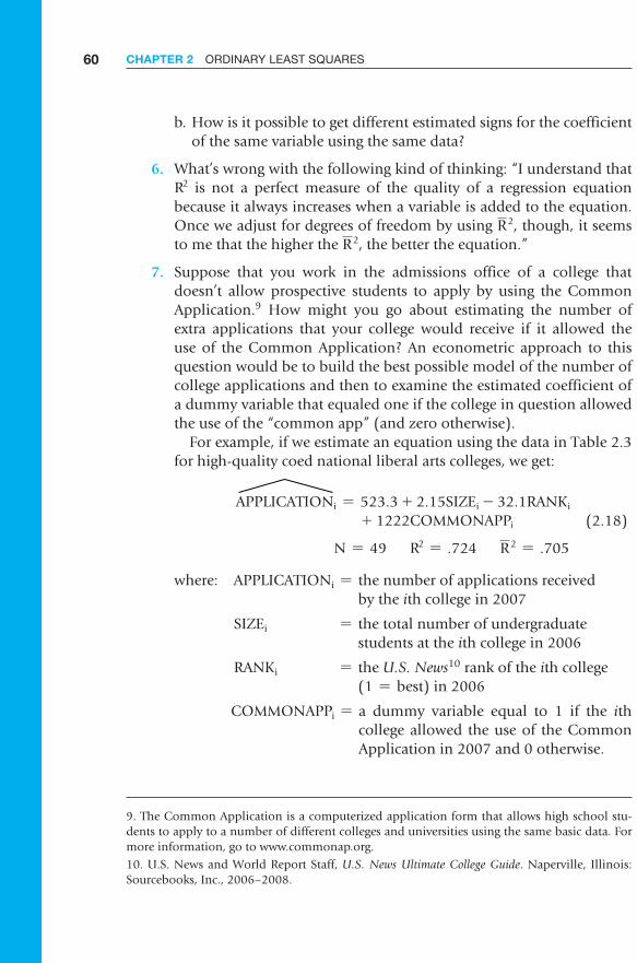
60 Chapter 2 OrdinAry LEAsT squArEs
b. How is it possible to get different estimated signs for the coefficient of the same variable using the same data?
6. What’s wrong with the following kind of thinking: “I understand that R2 is not a perfect measure of the quality of a regression equation because it always increases when a variable is added to the equation. Once we adjust for degrees of freedom by using R
2, though, it seems to me that the higher the R
2, the better the equation.”
7. Suppose that you work in the admissions office of a college that doesn’t allow prospective students to apply by using the Common Application.9 How might you go about estimating the number of extra applications that your college would receive if it allowed the use of the Common Application? An econometric approach to this question would be to build the best possible model of the number of college applications and then to examine the estimated coefficient of a dummy variable that equaled one if the college in question allowed the use of the “common app” (and zero otherwise).
For example, if we estimate an equation using the data in Table 2.3 for high-quality coed national liberal arts colleges, we get:
APPLICATIONi = 523.3 + 2.15SIZEi - 32.1RANKi
+ 1222COMMONAPPi (2.18)
N = 49 R2 = .724 R
2 = .705
where: APPLICATIONi = the number of applications received by the ith college in 2007
SIZEi = the total number of undergraduate students at the ith college in 2006
RANKi = the U.S. News10 rank of the ith college (1 = best) in 2006
COMMONAPPi = a dummy variable equal to 1 if the ith college allowed the use of the Common Application in 2007 and 0 otherwise.
9. The Common Application is a computerized application form that allows high school stu-dents to apply to a number of different colleges and universities using the same basic data. For more information, go to www.commonap.org.
10. U.S. News and World Report Staff, U.S. News Ultimate College Guide. Naperville, Illinois: Sourcebooks, Inc., 2006–2008.
M02_STUD2742_07_SE_C02.indd 60 19/01/16 4:50 PM
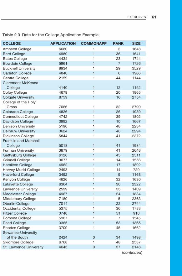
61eXerCises
Table 2.3 data for the College application example
COLLEGE AppLICAtION COMMONApp RANK SIZEamherst College 6680 1 2 1648bard College 4980 1 36 1641bates College 4434 1 23 1744bowdoin College 5961 1 7 1726bucknell university 8934 1 29 3529Carleton College 4840 1 6 1966Centre College 2159 1 44 1144Claremont mcKenna College
4140
1
12
1152
Colby College 4679 1 20 1865Colgate university 8759 1 16 2754College of the holy Cross
7066
1
32
2790
Colorado College 4826 1 26 1939Connecticut College 4742 1 39 1802davidson College 3992 1 10 1667denison university 5196 1 48 2234depauw university 3624 1 48 2294dickinson College 5844 1 41 2372Franklin and marshall College
5018
1
41
1984
Furman university 3879 1 41 2648gettysburg College 6126 1 45 2511grinnell College 3077 1 14 1556hamilton College 4962 1 17 1802harvey mudd College 2493 1 14 729haverford College 3492 1 9 1168Kenyon College 4626 1 32 1630Lafayette College 6364 1 30 2322Lawrence university 2599 1 53 1409macalester College 4967 1 24 1884middlebury College 7180 1 5 2363Oberlin College 7014 1 22 2744Occidental College 5275 1 36 1783pitzer College 3748 1 51 918pomona College 5907 1 7 1545reed College 3365 1 53 1365rhodes College 3709 1 45 1662sewanee-university of the south
2424
0
34
1498
skidmore College 6768 1 48 2537st. Lawrence university 4645 0 57 2148
(continued)
M02_STUD2742_07_SE_C02.indd 61 1/4/16 6:46 PM
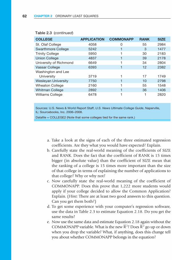
62 ChAptER 2 Ordinary Least squares
a. Take a look at the signs of each of the three estimated regression coefficients. Are they what you would have expected? Explain.
b. Carefully state the real-world meaning of the coefficients of SIZE and RANK. Does the fact that the coefficient of RANK is 15 times bigger (in absolute value) than the coefficient of SIZE mean that the ranking of a college is 15 times more important than the size of that college in terms of explaining the number of applications to that college? Why or why not?
c. Now carefully state the real-world meaning of the coefficient of COMMONAPP. Does this prove that 1,222 more students would apply if your college decided to allow the Common Application? Explain. (Hint: There are at least two good answers to this question. Can you get them both?)
d. To get some experience with your computer’s regression software, use the data in Table 2.3 to estimate Equation 2.18. Do you get the same results?
e. Now use the same data and estimate Equation 2.18 again without the COMMONAPP variable. What is the new R
2? Does R
2 go up or down when you drop the variable? What, if anything, does this change tell you about whether COMMONAPP belongs in the equation?
COLLEGE AppLICAtION COMMONApp RANK SIZEst. Olaf College 4058 0 55 2984swarthmore College 5242 1 3 1477trinity College 5950 1 30 2183union College 4837 1 39 2178university of richmond 6649 1 34 2804Vassar College 6393 1 12 2382washington and Lee university
3719
1
17
1749
wesleyan university 7750 1 10 2798wheaton College 2160 1 55 1548whitman College 2892 1 36 1406williams College 6478 1 1 2820
sources: u.s. news & world report staff, U.S. News Ultimate College Guide, naperville, iL: sourcebooks, inc. 2006–2008.
datafile = COLLege2 (note that some colleges tied for the same rank.)
Table 2.3 (continued)
M02_STUD2742_07_SE_C02.indd 62 1/4/16 6:46 PM
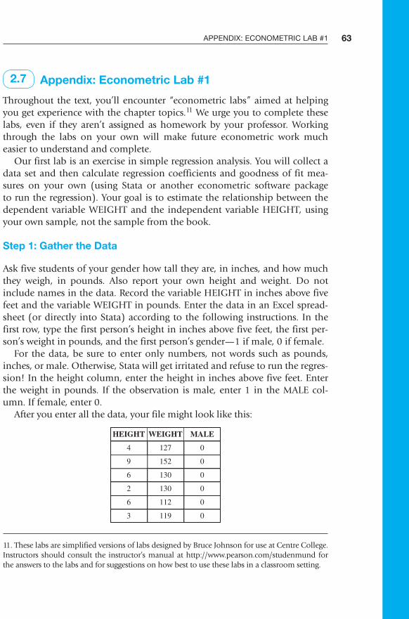
63 AppEndix: EcOnOmETric LAb #1
2.7 appendix: econometric Lab #1
Throughout the text, you’ll encounter “econometric labs” aimed at helping you get experience with the chapter topics.11 We urge you to complete these labs, even if they aren’t assigned as homework by your professor. Working through the labs on your own will make future econometric work much easier to understand and complete.
Our first lab is an exercise in simple regression analysis. You will collect a data set and then calculate regression coefficients and goodness of fit mea-sures on your own (using Stata or another econometric software package to run the regression). Your goal is to estimate the relationship between the dependent variable WEIGHT and the independent variable HEIGHT, using your own sample, not the sample from the book.
Step 1: Gather the Data
Ask five students of your gender how tall they are, in inches, and how much they weigh, in pounds. Also report your own height and weight. Do not include names in the data. Record the variable HEIGHT in inches above five feet and the variable WEIGHT in pounds. Enter the data in an Excel spread-sheet (or directly into Stata) according to the following instructions. In the first row, type the first person’s height in inches above five feet, the first per-son’s weight in pounds, and the first person’s gender—1 if male, 0 if female.
For the data, be sure to enter only numbers, not words such as pounds, inches, or male. Otherwise, Stata will get irritated and refuse to run the regres-sion! In the height column, enter the height in inches above five feet. Enter the weight in pounds. If the observation is male, enter 1 in the MALE col-umn. If female, enter 0.
After you enter all the data, your file might look like this:
HEIGHT WEIGHT MALE
4 127 0
9 152 0
6 130 0
2 130 0
6 112 0
3 119 0
11. These labs are simplified versions of labs designed by Bruce Johnson for use at Centre College. Instructors should consult the instructor’s manual at http://www.pearson.com/studenmund for the answers to the labs and for suggestions on how best to use these labs in a classroom setting.
M02_STUD2742_07_SE_C02.indd 63 19/01/16 4:50 PM
64 Chapter 2 Ordinary Least squares
Now carry out the following tasks and answer the questions in order, using the data you collected.
Step 2: Calculate Summary Statistics
Use Stata to compute the summary statistics. What is the mean? Also look at the minimum, the maximum, and the sample size.
Step 3: run the regression
Run the regression in Stata. Can you find the estimated βs? Print the regression results if you are doing this lab as a class assignment.
Step 4: Interpret the estimated Coefficients
State the precise meaning of the slope coefficient. Now compare your esti-mated coefficients with those in Equation 2.6. Are your results the same? If not, do you understand why they’re different?
Step 5: Interpret r
2
Can you find R
2 in your results? What is it? State precisely the meaning of the R
2 statistic.
Step 6: estimate a Second equation
Now add MALE to your equation as a second independent variable and esti-mate it again. Do you see a problem? Explain. Does this imply that gender has no relationship to weight?
M02_STUD2742_07_SE_C02.indd 64 21/01/16 2:40 PM

65
3.1 Steps in Applied Regression Analysis
3.2 Using Regression Analysis to Pick Restaurant Locations
3.3 Dummy Variables
3.4 Summary and Exercises
3.5 Appendix: Econometric Lab #2
Learning to Use Regression Analysis
From a quick reading of Chapter 2, it’d be easy to conclude that regression analysis is little more than the mechanical application of a set of equations to a sample of data. Such a notion would be similar to deciding that all that matters in golf is hitting the ball well. Golfers will tell you that it does little good to hit the ball well if you have used the wrong club or have hit the ball toward a trap, tree, or pond. Similarly, experienced econometricians spend much less time thinking about the OLS estimation of an equation than they do about a number of other factors. Our goal in this chapter is to introduce some of these “real-world” concerns.
The first section, an overview of the six steps typically taken in applied regression analysis, is the most important in the chapter. We believe that the ability to learn and understand a specific topic, like OLS estimation, is enhanced if the reader has a clear vision of the role that the specific topic plays in the overall framework of regression analysis. In addition, the six steps make it hard to miss the crucial function of theory in the development of sound econometric research.
This is followed by a complete example of how to use the six steps in applied regression: a location analysis for the “Woody’s” restaurant chain that is based on actual company data and to which we will return in future chapters to apply new ideas and tests. The chapter concludes with a discus-sion of dummy variables and econometric lab #2.
Chapter 3
M03_STUD2742_07_SE_C03.indd 65 1/4/16 6:10 PM

66 ChAPtER 3 Learning to Use regression anaLysis
3.1 Steps in Applied Regression Analysis
Although there are no hard and fast rules for conducting econometric research, most investigators commonly follow a standard method for applied regression analysis. The relative emphasis and effort expended on each step will vary, but normally all the steps are necessary for successful research. Note that we don’t discuss the selection of the dependent variable; this choice is determined by the purpose of the research. We’ll cover choosing a dependent variable in Chapter 11. Once a dependent variable is chosen, however, it’s logical to follow these six steps in applied regression analysis.
1. Review the literature and develop the theoretical model.
2. Specify the model: Select the independent variables and the functional form.
3. Hypothesize the expected signs of the coefficients.
4. Collect the data. Inspect and clean the data.
5. Estimate and evaluate the equation.
6. Document the results.
The purpose of suggesting these steps is not to discourage the use of innova-tive or unusual approaches but rather to develop in the reader a sense of how regression ordinarily is done by professional economists and business analysts.
Step 1: Review the Literature and Develop the theoretical Model
The first step in any applied research is to get a good theoretical grasp of the topic to be studied. That’s right: the best data analysts don’t start with data, but with theory! This is because many econometric decisions, ranging from which variables to include to which functional form to employ, are determined by the underlying theoretical model. It’s virtually impossible to build a good econo-metric model without a solid understanding of the topic you’re studying.
For most topics, this means that it’s smart to review the scholarly literature before doing anything else. If a professor has investigated the theory behind your topic, you want to know about it. If other researchers have estimated equations for your dependent variable, you might want to apply one of their models to your data set. On the other hand, if you disagree with the approach of previous authors, you might want to head off in a new direction. In either case, you shouldn’t have to “reinvent the wheel.” You should start
M03_STUD2742_07_SE_C03.indd 66 1/4/16 6:10 PM

67 steps in appLied regression anaLysis
your investigation where earlier researchers left off. Any academic paper on an empirical topic should begin with a summary of the extent and quality of previous research.
The most convenient approaches to reviewing the literature are to obtain several recent issues of the Journal of Economic Literature or a business-oriented publication of abstracts, or to run an Internet search or an EconLit search1 on your topic. Using these resources, find and read several recent articles on your topic. Pay attention to the bibliographies of these articles. If an older article is cited by a number of current authors, or if its title hits your topic on the head, trace back through the literature and find this article as well. We’ll have more advice on reviewing the literature in Chapter 11.
In some cases, a topic will be so new or so obscure that you won’t be able to find any articles on it. What then? We recommend two possible strategies. First, try to transfer theory from a similar topic to yours. For example, if you’re trying to build a model of the demand for a new product, read articles that analyze the demand for similar, existing products. Second, if all else fails, contact someone who works in the field you’re investigating. For example, if you’re building a model of housing in an unfamiliar city, call a real estate agent who works there.
Step 2: Specify the Model: Select the Independent Variables and the Functional Form
The most important step in applied regression analysis is the specification of the theoretical regression model. After selecting the dependent variable, the specification of a model involves choosing the following components:
1. the independent variables and how they should be measured,
2. the functional (mathematical) form of the variables, and
3. the properties of the stochastic error term.
A regression equation is specified when each of these elements has been treated appropriately. We’ll discuss the details of these specification decisions in Chapters 6, 7, and 4, respectively.
Each of the elements of specification is determined primarily on the basis of economic theory. A mistake in any of the three elements results in a
1. EconLit is an electronic bibliography of economics literature. EconLit contains abstracts, reviews, indexing, and links to full-text articles in economics journals. In addition, it abstracts books and indexes articles in books, working papers series, and dissertations. EconLit is available at libraries and on university websites throughout the world. For more, go to www. EconLit.org.
M03_STUD2742_07_SE_C03.indd 67 1/4/16 6:10 PM

68 ChAPtER 3 Learning to Use regression anaLysis
specification error. Of all the kinds of mistakes that can be made in applied regression analysis, specification error is usually the most disastrous to the validity of the estimated equation. Thus, the more attention paid to eco-nomic theory at the beginning of a project, the more satisfying the regression results are likely to be.
The emphasis in this text is on estimating behavioral equations, those that describe the behavior of economic entities. We focus on selecting inde-pendent variables based on the economic theory concerning that behavior. An explanatory variable is chosen because it is a theoretical determinant of the dependent variable; it is expected to explain at least part of the varia-tion in the dependent variable. Recall that regression gives evidence but does not prove economic causality. Just as an example does not prove the rule, a regression result does not prove the theory.
There are dangers in specifying the wrong independent variables. Our goal should be to specify only relevant explanatory variables, those expected theoretically to assert a substantive influence on the dependent variable. Vari-ables suspected of having little effect should be excluded unless their possible impact on the dependent variable is of some particular (e.g., policy) interest.
For example, an equation that explains the quantity demanded of a con-sumption good might use the price of the product and consumer income or wealth as likely variables. Theory also indicates that complementary and sub-stitute goods are important. Therefore, you might decide to include the prices of complements and substitutes, but which complements and substitutes? Of course, selection of the closest complements and/or substitutes is appro-priate, but how far should you go? The choice must be based on theoretical judgment, and such judgments are often quite subjective.
When researchers decide, for example, that the prices of only two other goods need to be included, they are said to impose their priors (i.e., previous theoretical belief) or their working hypotheses on the regression equation. Imposition of such priors is a common practice that determines the number and kind of hypotheses that the regression equation has to test. The danger is that a prior may be wrong and could diminish the usefulness of the esti-mated regression equation. Each of the priors therefore should be explained and justified in detail.
Step 3: hypothesize the Expected Signs of the Coefficients
Once the variables have been selected, it’s important to hypothesize the expected signs of the slope coefficients before you collect any data. In many cases, the basic theory is general knowledge, so you don’t need to discuss the reasons for the expected sign. However, if any doubt surrounds the choice of
M03_STUD2742_07_SE_C03.indd 68 1/4/16 6:10 PM

69 steps in appLied regression anaLysis
an expected sign, then you should document the opposing theories and your reasons for hypothesizing a positive or a negative slope2 coefficient.
For example, suppose that you’re interested in the impact of class size on student learning at the elementary level in the United States. A reasonable dependent variable 1Y2 might be the student score on a test of grammar, math, and science. Likely independent variables would include the income level of the student’s family 1X12 and the size (in students per teacher) of the student’s class 1X22.
+ - Y = β0 + β1X1 + β2X2 + e (3.1)
The signs above the coefficients in Equation 3.1 indicate the hypothesized sign of that particular coefficient. Take another look at the equation. Do you agree with the hypothesized signs? The expectation that higher income will improve test scores (holding constant class size) seems reasonable because of the extra learning opportunities that the money might allow, but the hypoth-esized sign for β2 is a little trickier. Do you agree that it should be negative?
Step 4: Collect the Data. Inspect and Clean the Data
Obtaining an original data set and properly preparing it for regression is a surprisingly difficult task. This step entails more than a mechanical recording of data, because the type and size of the sample also must be chosen.
A general rule regarding sample size is “the more observations the better,” as long as the observations are from the same general population. Ordinarily, researchers take all the roughly comparable observations that are readily available. In regression analysis, all the variables must have the same number of observations. They also should have the same frequency (monthly, quar-terly, annual, etc.) and time period. Often, the frequency selected is deter-mined by the availability of data.
The reason there should be as many observations as possible concerns the statistical concept of degrees of freedom first mentioned in Section 2.4. Consider fitting a straight line to two points on an X, Y coordinate system as in Figure 3.1. Such an exercise can be done mathematically without error. Both points lie on the line, so there is no estimation of the coefficients involved. The two points determine the two parameters, the intercept and the slope, precisely. Estimation takes place only when a straight line is fitted to
2. Note that while we hypothesize signs for the slope coefficients, we don’t hypothesize an expected sign for the intercept. We’ll explain why in Section 7.1.
M03_STUD2742_07_SE_C03.indd 69 1/4/16 6:10 PM
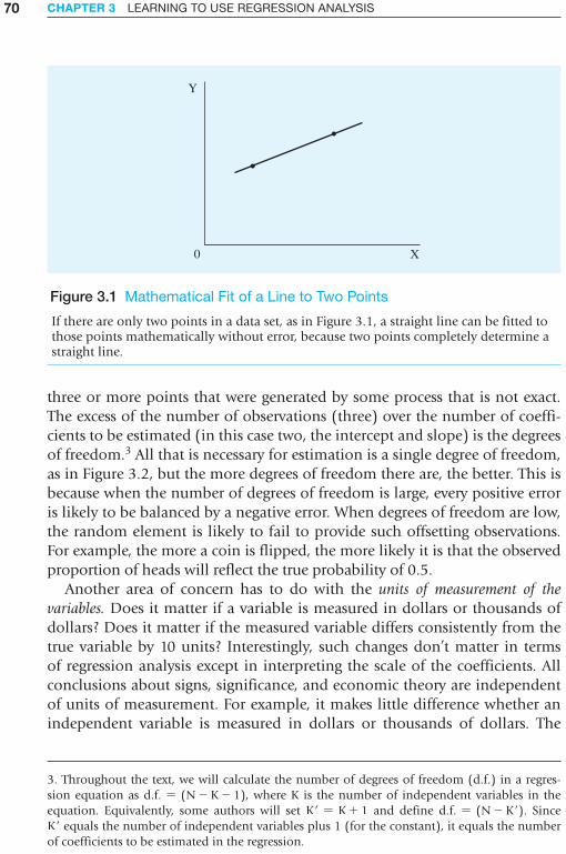
70 ChAPtER 3 Learning to Use regression anaLysis
three or more points that were generated by some process that is not exact. The excess of the number of observations (three) over the number of coeffi-cients to be estimated (in this case two, the intercept and slope) is the degrees of freedom.3 All that is necessary for estimation is a single degree of freedom, as in Figure 3.2, but the more degrees of freedom there are, the better. This is because when the number of degrees of freedom is large, every positive error is likely to be balanced by a negative error. When degrees of freedom are low, the random element is likely to fail to provide such offsetting observations. For example, the more a coin is flipped, the more likely it is that the observed proportion of heads will reflect the true probability of 0.5.
Another area of concern has to do with the units of measurement of the variables. Does it matter if a variable is measured in dollars or thousands of dollars? Does it matter if the measured variable differs consistently from the true variable by 10 units? Interestingly, such changes don’t matter in terms of regression analysis except in interpreting the scale of the coefficients. All conclusions about signs, significance, and economic theory are independent of units of measurement. For example, it makes little difference whether an independent variable is measured in dollars or thousands of dollars. The
3. Throughout the text, we will calculate the number of degrees of freedom (d.f.) in a regres-sion equation as d.f. = (N - K - 1), where K is the number of independent variables in the equation. Equivalently, some authors will set K′ = K + 1 and define d.f. = (N - K′). Since K′ equals the number of independent variables plus 1 (for the constant), it equals the number of coefficients to be estimated in the regression.
Y
0 X
Figure 3.1 Mathematical Fit of a Line to two points
If there are only two points in a data set, as in Figure 3.1, a straight line can be fitted to those points mathematically without error, because two points completely determine a straight line.
M03_STUD2742_07_SE_C03.indd 70 1/4/16 6:10 PM

71 steps in appLied regression anaLysis
constant term and measures of overall fit remain unchanged. Such a multipli-cative factor does change the slope coefficient, but only by the exact amount necessary to compensate for the change in the units of measurement of the independent variable. Similarly, a constant factor added to a variable alters only the intercept term without changing the slope coefficient itself.
The final step before estimating your equation is to inspect and clean the data. You should make it a point always to look over your data set to see if you can find any errors. The reason is obvious: why bother using sophisti-cated regression analysis if your data are incorrect?
To inspect the data, obtain a plot (graph) of the data and look for outliers. An outlier is an observation that lies outside the range of the rest of the observa-tions, and looking for outliers is an easy way to find data entry errors. In addi-tion, it’s a good habit to look at the mean, maximum, and minimum of each variable and then think about possible inconsistencies in the data. Are any observations impossible or unrealistic? Did GDP double in one year? Does a student have a 7.0 GPA on a 4.0 scale? Is consumption negative?
Typically, the data can be cleaned of these errors by replacing an incorrect number with the correct one. In extremely rare circumstances, an observation can be dropped from the sample, but only if the correct number can’t be found or if that particular observation clearly isn’t from the same population as the rest of the sample. Be careful! The mere existence of an outlier is not a justification for dropping that observation from the sample. A regression needs to be able to explain all the observations in a sample, not just the well-behaved ones. For more on the details of data collection, see Sections 11.2 and 11.3. For more on generating your own data through an economic experiment, see Section 16.1.
Y
0 X
Figure 3.2 statistical Fit of a Line to three points
If there are three (or more) points in a data set, as in Figure 3.2, then the line must almost always be fitted to the points statistically, using the estimation procedures of Section 2.1.
M03_STUD2742_07_SE_C03.indd 71 1/4/16 6:10 PM

72 ChAPtER 3 Learning to Use regression anaLysis
Step 5: Estimate and Evaluate the Equation
Believe it or not, it can take months to complete steps 1–4 for a regression equation, but a computer program like Stata or EViews can estimate that equa-tion in less than a second! Typically, estimation is done using OLS, as discussed in Section 2.1, but if another estimation technique is used, the reasons for that alternative technique should be carefully explained and evaluated.
You might think that once your equation has been estimated, your work is finished, but that’s hardly the case. Instead, you need to evaluate your results in a variety of ways. How well did the equation fit the data? Were the signs and magnitudes of the estimated coefficients what you expected? Most of the rest of this book is concerned with the evaluation of estimated econometric equations, and beginning researchers should be prepared to spend a consid-erable amount of time doing this evaluation.
Once this evaluation is complete, don’t automatically go to step 6. Regres-sion results are rarely what one expects, and additional model development often is required. For example, an evaluation of your results might indicate that your equation is missing an important variable. In such a case, you’d go back to step 1 to review the literature and add the appropriate variable to your equation. You’d then go through each of the steps in order until you had estimated your new specification in step 5. You’d move on to step 6 only if you were satisfied with your estimated equation. Don’t be too quick to make such adjustments, however, because we don’t want to adjust the theory merely to fit the data. A researcher has to walk a fine line between making appropriate changes and avoiding inappropriate ones, and making these choices is one of the artistic elements of applied econometrics.
Finally, it’s often worthwhile to estimate additional specifications of an equation in order to see how stable your observed results are. This approach, called sensitivity analysis, will be discussed in Section 6.4.
Step 6: Document the Results
A standard format usually is used to present estimated regression results:
Yni = 103.40 + 6.38Xi (0.88) (3.2) t = 7.22 N = 20 R
2 = .73
The number in parentheses is the estimated standard error of the estimated coefficient, and the t-value is the one used to test the hypothesis that the true value of the coefficient is different from zero. These and other measures
M03_STUD2742_07_SE_C03.indd 72 1/4/16 6:10 PM

73 Using regression anaLysis to pick restaUrant Locations
of the quality of the regression will be discussed in later chapters.4 What is important to note is that the documentation of regression results using an easily understood format is considered part of the analysis itself. For time-series data sets, the documentation also includes the frequency (e.g., quarterly or annual) and the time period of the data.
One of the important parts of the documentation is the explanation of the model, the assumptions, and the procedures and data used. The written doc-umentation must contain enough information so that the entire study could be replicated by others.5 Unless the variables have been defined in a glossary or table, short definitions should be presented along with the equations. If there is a series of estimated regression equations, then tables should provide the relevant information for each equation. All data manipulations as well as data sources should be documented fully. When there is much to explain, this documentation usually is relegated to a data appendix. If the data are not available generally or are available only after computation, the data set itself might be included in this appendix.
3.2 Using Regression Analysis to Pick Restaurant Locations
To solidify your understanding of the six basic steps of applied regression analysis, let’s work through a complete regression example. Suppose that you’ve been hired to determine the best location for the next Woody’s res-taurant, where Woody’s is a moderately priced, 24-hour, family restaurant chain.6 You decide to build a regression model to explain the gross sales vol-ume at each of the restaurants in the chain as a function of various descrip-tors of the location of that branch. If you can come up with a sound equation to explain gross sales as a function of location, then you can use this equa-tion to help Woody’s decide where to build their newest eatery. Given data on
4. The standard error of the coefficient is discussed in more detail in Section 4.2; the t-value is developed in Section 5.2. 5. For example, the Journal of Money, Credit, and Banking and the American Economic Review have requested authors to submit their actual data sets so that regression results can be verified. See W. G. Dewald et al., “Replication in Empirical Economics,” American Economic Review, Vol. 76, No. 4, pp. 587–603 and Daniel S. Hamermesh, “Replication in Economics,” NBER Working Paper 13026, April 2007.6. The data in this example are real (they’re from a sample of 33 Denny’s restaurants in Southern California), but the number of independent variables considered is much smaller than was used in the actual research. Datafile = WOODY3.
M03_STUD2742_07_SE_C03.indd 73 1/4/16 6:10 PM
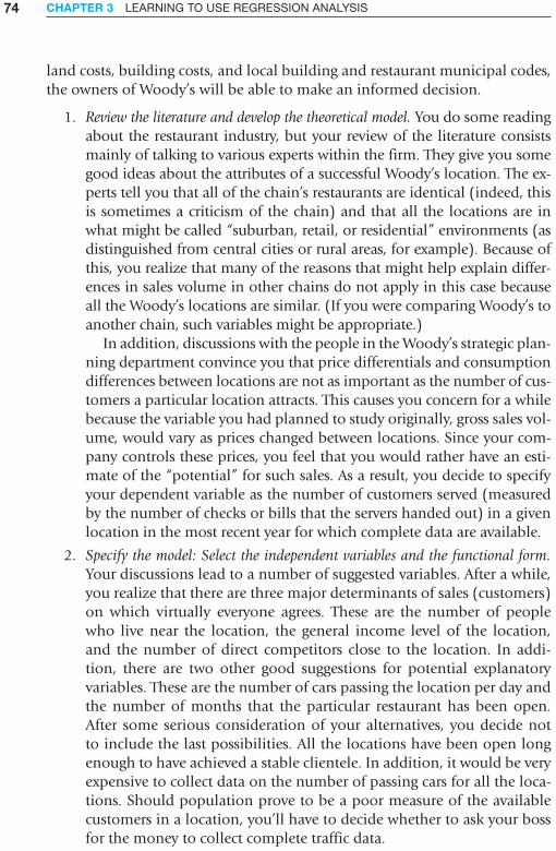
74 ChAPtER 3 Learning to Use regression anaLysis
land costs, building costs, and local building and restaurant municipal codes, the owners of Woody’s will be able to make an informed decision.
1. Review the literature and develop the theoretical model. You do some reading about the restaurant industry, but your review of the literature consists mainly of talking to various experts within the firm. They give you some good ideas about the attributes of a successful Woody’s location. The ex-perts tell you that all of the chain’s restaurants are identical (indeed, this is sometimes a criticism of the chain) and that all the locations are in what might be called “suburban, retail, or residential” environments (as distinguished from central cities or rural areas, for example). Because of this, you realize that many of the reasons that might help explain differ-ences in sales volume in other chains do not apply in this case because all the Woody’s locations are similar. (If you were comparing Woody’s to another chain, such variables might be appropriate.)
In addition, discussions with the people in the Woody’s strategic plan-ning department convince you that price differentials and consumption differences between locations are not as important as the number of cus-tomers a particular location attracts. This causes you concern for a while because the variable you had planned to study originally, gross sales vol-ume, would vary as prices changed between locations. Since your com-pany controls these prices, you feel that you would rather have an esti-mate of the “potential” for such sales. As a result, you decide to specify your dependent variable as the number of customers served (measured by the number of checks or bills that the servers handed out) in a given location in the most recent year for which complete data are available.
2. Specify the model: Select the independent variables and the functional form. Your discussions lead to a number of suggested variables. After a while, you realize that there are three major determinants of sales (customers) on which virtually everyone agrees. These are the number of people who live near the location, the general income level of the location, and the number of direct competitors close to the location. In addi-tion, there are two other good suggestions for potential explanatory variables. These are the number of cars passing the location per day and the number of months that the particular restaurant has been open. After some serious consideration of your alternatives, you decide not to include the last possibilities. All the locations have been open long enough to have achieved a stable clientele. In addition, it would be very expensive to collect data on the number of passing cars for all the loca-tions. Should population prove to be a poor measure of the available customers in a location, you’ll have to decide whether to ask your boss for the money to collect complete traffic data.
M03_STUD2742_07_SE_C03.indd 74 1/4/16 6:10 PM

75 Using regression anaLysis to pick restaUrant Locations
The exact definitions of the independent variables you decide to include are:
N = Competition: the number of direct market competitors within a two-mile radius of the Woody’s location
P = Population: the number of people living within a three-mile radius of the Woody’s location
I = Income: the average household income of the population measured in variable P
Since we have yet to develop any functional forms other than a linear functional form and a typical stochastic error term, that’s what you decide to use.
3. Hypothesize the expected signs of the coefficients. After thinking about which variables to include, you expect hypothesizing signs will be easy. For two of the variables, you’re right. Everyone expects that the more competition there is, the fewer customers (holding constant the popu-lation and income of an area) there will be, and also that the more people there are who live near a particular restaurant, the more cus-tomers (holding constant the competition and income) the restaurant will have. You expect that the greater the income is in a particular area, the more people will choose to eat in a family restaurant. However, people in especially high-income areas might want to eat in a restau-rant that has more “atmosphere” than a family restaurant like Woody’s. As a result, you worry that the income variable might be only weakly positive in its impact. To sum, you expect:
- + +? Yi = β0 + βNNi + βPPi + βIIi + ei (3.3)
where the signs above the coefficients indicate the expected impact of that particular independent variable on the dependent variable, hold-ing constant the other two explanatory variables, and ei is a typical sto-chastic error term.
4. Collect the data. Inspect and clean the data. You want to include every local restaurant in the Woody’s chain in your study, and, after some effort, you come up with data for your dependent variable and your independent variables for all 33 locations. You inspect the data, and you’re confident that the quality of your data is excellent for three rea-sons: each manager measured each variable identically, you’ve included each restaurant in the sample, and all the information is from the same year. [The data set is included in this section, along with a sample com-puter output for the regression estimated by Stata (Tables 3.1 and 3.2).]
M03_STUD2742_07_SE_C03.indd 75 1/4/16 6:10 PM

76 ChAPtER 3 Learning to Use regression anaLysis
Table 3.1 data for the Woody’s restaurant example (Using the stata program)
y n p i
1. 107919 3 65044 132402. 118866 5 101376 225543. 98579 7 124989 169164. 122015 2 55249 209675. 152827 3 73775 19576
6. 91259 5 48484 150397. 123550 8 138809 218578. 160931 2 50244 264359. 98496 6 104300 24024
10. 108052 2 37852 14987
11. 144788 3 66921 3090212. 164571 4 166332 3157313. 105564 3 61951 1900114. 102568 5 100441 2005815. 103342 2 39462 16194
16. 127030 5 139900 2138417. 166755 6 171740 1880018. 125343 6 149894 1528919. 121886 3 57386 1670220. 134594 6 185105 19093
21. 152937 3 114520 2650222. 109622 3 52933 1876023. 149884 5 203500 3324224. 98388 4 39334 1498825. 140791 3 95120 18505
26. 101260 3 49200 1683927. 139517 4 113566 2891528. 115236 9 194125 1903329. 136749 7 233844 1920030. 105067 7 83416 22833
31. 136872 6 183953 1440932. 117146 3 60457 2030733. 163538 2 65065 20111
(obs=33)
y n p i
y 1.0000n -0.1442 1.0000p 0.3926 0.7263 1.0000i 0.5370 -0.0315 0.2452 1.0000
M03_STUD2742_07_SE_C03.indd 76 1/4/16 6:10 PM

77 Using regression anaLysis to pick restaUrant Locations
Table 3.2 actual computer output (Using the stata program)
number of obs = 33F( 3, 29) = 15.65prob 7 F = 0.0000r–squared = 0.6182adj r–squared = 0.5787root Mse = 14543
y coef. std. err. t p 7 � t � [95% conf. interval]
n -9074.674 2052.674 -4.42 0.000 -13272.86 -4876.485p .3546684 .0726808 4.88 0.000 .2060195 .5033172i 1.287923 .5432938 2.37 0.025 .1767628 2.399084
_cons 102192.4 12799.83 7.98 0.000 76013.84 128371
source ss df Ms
Model 9.9289e + 09 3 3.3096e + 09residual 6.1333e + 09 29 211492485
total 1.6062e + 10 32 501943246
y yhat residuals
1. 107919 115089.6 -7170.562. 118866 121821.7 -2955.743. 98579 104785.9 -6206.8644. 122015 130642 -8627.0415. 152827 126346.5 26480.55
6. 91259 93383.88 -2124.8777. 123550 106976.3 16573.668. 160931 135909.3 25021.719. 98496 115677.4 -17181.36
10. 108052 116770.1 -8718.094
11. 144788 138502.6 6285.42512. 164571 165550 -979.034213. 105564 121412.3 -15848.314. 102568 118275.5 -15707.4715. 103342 118895.6 -15553.63
16. 127030 133978.1 -6948.11417. 166755 132868.1 33886.9118. 125343 120598.1 4744.89819. 121886 116832.3 5053.720. 134594 137985.6 -3391.591
21. 152937 149717.6 3219.42822. 109622 117903.5 -8281.50823. 149884 171807.2 -21923.2224. 98388 99147.65 -759.651425. 140791 132537.5 8253.518
26. 101260 114105.4 -12845.4327. 139517 143412.3 -3895.30328. 115236 113883.4 1352.59929. 136749 146334.9 -9585.90530. 105067 97661.88 7405.122
31. 136872 131544.4 5327.62132. 117146 122564.5 -5418.4533. 163538 133021 30517
M03_STUD2742_07_SE_C03.indd 77 1/4/16 6:10 PM
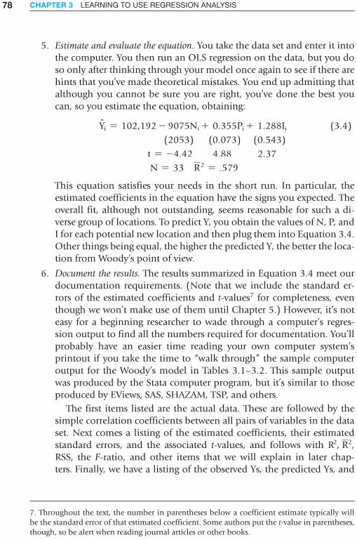
78 ChAPtER 3 Learning to Use regression anaLysis
5. Estimate and evaluate the equation. You take the data set and enter it into the computer. You then run an OLS regression on the data, but you do so only after thinking through your model once again to see if there are hints that you’ve made theoretical mistakes. You end up admitting that although you cannot be sure you are right, you’ve done the best you can, so you estimate the equation, obtaining:
Yni = 102,192 - 9075Ni + 0.355Pi + 1.288Ii (3.4) (2053) (0.073) (0.543) t = -4.42 4.88 2.37 N = 33 R
2 = .579
This equation satisfies your needs in the short run. In particular, the estimated coefficients in the equation have the signs you expected. The overall fit, although not outstanding, seems reasonable for such a di-verse group of locations. To predict Y, you obtain the values of N, P, and I for each potential new location and then plug them into Equation 3.4. Other things being equal, the higher the predicted Y, the better the loca-tion from Woody’s point of view.
6. Document the results. The results summarized in Equation 3.4 meet our documentation requirements. (Note that we include the standard er-rors of the estimated coefficients and t-values7 for completeness, even though we won’t make use of them until Chapter 5.) However, it’s not easy for a beginning researcher to wade through a computer’s regres-sion output to find all the numbers required for documentation. You’ll probably have an easier time reading your own computer system’s printout if you take the time to “walk through” the sample computer output for the Woody’s model in Tables 3.1–3.2. This sample output was produced by the Stata computer program, but it’s similar to those produced by EViews, SAS, SHAZAM, TSP, and others.
7. Throughout the text, the number in parentheses below a coefficient estimate typically will be the standard error of that estimated coefficient. Some authors put the t-value in parentheses, though, so be alert when reading journal articles or other books.
The first items listed are the actual data. These are followed by the simple correlation coefficients between all pairs of variables in the data set. Next comes a listing of the estimated coefficients, their estimated standard errors, and the associated t-values, and follows with R2, R2, RSS, the F-ratio, and other items that we will explain in later chap-ters. Finally, we have a listing of the observed Ys, the predicted Ys, and
M03_STUD2742_07_SE_C03.indd 78 1/4/16 6:10 PM

79 dUMMy VariabLes
the residuals for each observation. Numbers followed by “e + 06” or “e - 01” are expressed in a scientific notation indicating that the printed decimal point should be moved six places to the right or one place to the left, respectively.
In future sections, we’ll return to this example in order to apply vari-ous tests and ideas as we learn them.
3.3 Dummy Variables
Some concepts (for example, gender) might seem impossible to include in an equation because they’re inherently qualitative in nature and can’t be expressed as a number. Luckily, such concepts can be quantified by using dummy (or binary) variables. A dummy variable takes on the value of one or zero (and only those values) depending on whether a specified condition is met.
As an illustration of a dummy variable, suppose that Yi represents the salary of the ith high school teacher and that salaries depend primarily on the experience of the teacher and the type of degree that the teacher has earned. All teachers have a B.A., but some also have a graduate degree like an M.A. An equation representing the relationship between earnings and these variables would be:
+ + Yi = β0 + β1Xi + β2Di + ei (3.5)
where: Yi = the income of the ith teacher in dollars Xi = the number of years of teaching experience of the ith
teacher
Di = e1 if the ith teacher has a graduate degree0 otherwise
The variable Di takes on values of only zero or one, so Di is called a dummy variable, or just a “dummy.” Needless to say, the term has generated many a pun. In this case, the dummy variable represents the condition of having a graduate degree. The coefficient β2 indicates the additional salary that can be attributed to having a graduate degree, holding teaching experi-ence constant.
Since more experience and a graduate degree can be expected to increase the earnings of teachers, we expect positive coefficients for both variables, as indicated by the signs above the coefficients in Equation 3.5. Think for a second about what those expected signs would be if we had instead
M03_STUD2742_07_SE_C03.indd 79 1/4/16 6:10 PM
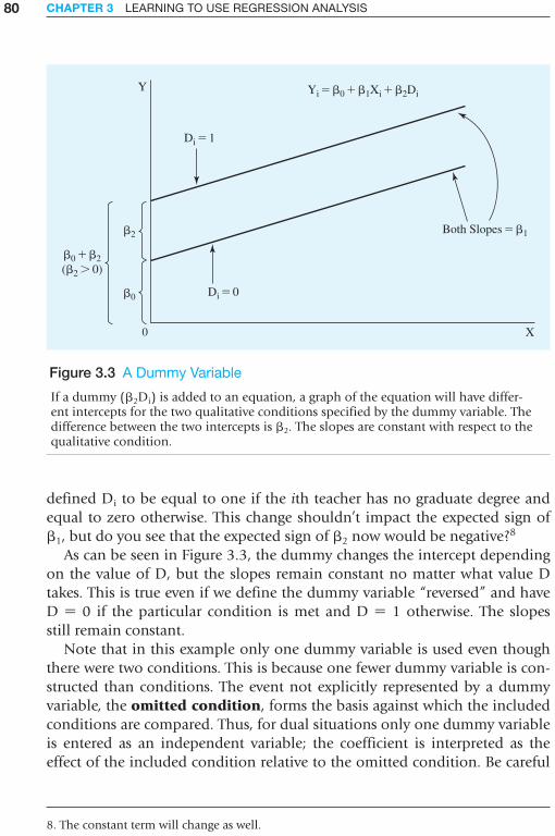
80 ChAPtER 3 Learning to Use regression anaLysis
defined Di to be equal to one if the ith teacher has no graduate degree and equal to zero otherwise. This change shouldn’t impact the expected sign of β1, but do you see that the expected sign of β2 now would be negative?8
As can be seen in Figure 3.3, the dummy changes the intercept depending on the value of D, but the slopes remain constant no matter what value D takes. This is true even if we define the dummy variable “reversed” and have D = 0 if the particular condition is met and D = 1 otherwise. The slopes still remain constant.
Note that in this example only one dummy variable is used even though there were two conditions. This is because one fewer dummy variable is con-structed than conditions. The event not explicitly represented by a dummy variable, the omitted condition, forms the basis against which the included conditions are compared. Thus, for dual situations only one dummy variable is entered as an independent variable; the coefficient is interpreted as the effect of the included condition relative to the omitted condition. Be careful
Y
0 X
Di = 0
d2
d0
d0 + d2(d2 7 0)
Di = 1
Both Slopes = d1
Yi = d0 + d1Xi + d2Di
Figure 3.3 a dummy Variable
If a dummy (β2Di) is added to an equation, a graph of the equation will have differ-ent intercepts for the two qualitative conditions specified by the dummy variable. The difference between the two intercepts is β2. The slopes are constant with respect to the qualitative condition.
8. The constant term will change as well.
M03_STUD2742_07_SE_C03.indd 80 1/4/16 6:10 PM

81 dUMMy VariabLes
never to use two dummy variables to describe the two conditions. If you were to make this mistake, sometimes called a dummy variable trap, you’d have per-fect multicollinearity (to be described in Section 8.1).
For another example of the meaning of the coefficient of a dummy vari-able, let’s look at a study of the relationship between fraternity/sorority mem-bership and grade point average (GPA). Most noneconometricians would approach this research problem by calculating the mean grades of fraternity/sorority (so-called Greek) members and comparing them to the mean grades of nonmembers. However, such a technique would ignore the relationship that grades have to characteristics other than Greek membership.
Instead, we’d want to build a regression model that explains college GPA. Independent variables would include not only Greek membership but also other predictors of academic performance such as SAT scores and high school grades. Being a member of a social organization is a qualitative variable, however, so we’d have to create a dummy variable to represent fraternity or sorority membership quantitatively in a regression equation:
Di = • 1 if the ith student is an active member of a fraternity or sorority 0 otherwise
If we collect data from all the students in our class and estimate the equa-tion implied in this example, we obtain:
CGi = 0.37 + 0.81HGi + 0.00001Si - 0.38Di (3.6) R
2 = .45 N = 25
where: CGi = the cumulative college GPA (4-point scale) of the ith student
HGi = the cumulative high school GPA (4-point scale) of the ith student
Si = the sum of the highest verbal and mathematics SAT scores earned by the ith student
The meaning of the estimated coefficient of Di in Equation 3.6 is very spe-cific. Stop for a second and figure it out for yourself. What is it? The estimate that βnD = -0.38 means that, for this sample, the GPA of fraternity/sorority members is 0.38 lower than for nonmembers, holding SATs and high school GPA constant. Thus, Greek members are doing about a third of a grade worse than otherwise might be expected. To understand this example better, try using Equation 3.6 to predict your own GPA; how close does it come?
h
M03_STUD2742_07_SE_C03.indd 81 1/4/16 6:10 PM

82 ChAPtER 3 Learning to Use regression anaLysis
Before you rush out and quit whatever social organization you’re in, how-ever, note that this sample is quite small and that we’ve surely omitted some important determinants of academic success from the equation. As a result, we shouldn’t be too quick to conclude that Greeks are dummies.
Up to this point, we’ve used dummy variables to represent only those qualitative variables that have exactly two possibilities (such as gender). What about situations where a qualitative variable has three or more alternatives? For example, in our study of the salaries of high school teachers in Equation 3.5, what if we learn that some of the teachers have Ph.D.s? We now need to be able to distinguish teachers whose highest degree is a Ph.D. from teachers whose highest degree is an M.A. from teachers whose highest degree is a B.A. What can we do?
Well, the answer certainly isn’t to define a variable such that Ph.D. = 2, M.A. = 1, and B.A. = 0, because we have no reason to think that the impact of having a Ph.D. is exactly twice that of having an M.A. If not that, then what?
The answer is to create one fewer dummy variable than there are pos-sibilities (conditions) and to use each dummy to represent only one of the possible conditions. In the high school salary case, you’d create two dummy variables to represent the three conditions, for example:
PHDi = e1 if the ith teacher’s highest degree is a Ph.D.0 otherwise
and
MAi = e1 if the ith teacher’s highest degree is an M.A.0 otherwise
The omitted condition (when a B.A. is the highest degree) is represented by having both dummies equal to 0. This way you can measure the impact of each degree independently without having to link the impacts of having an M.A. and a Ph.D.
Thus Equation 3.5 now would look like this:
+ + ? Yi = β0 + β1Xi + β2PHDi + β3MAi + ei (3.7)
However, be careful! The interpretation of the coefficients when there are two or more related dummy variables is tricky. The coefficient tells you the increase in the dependent variable caused by the condition being met
M03_STUD2742_07_SE_C03.indd 82 1/4/16 6:10 PM

83 sUMMary
compared to the omitted condition. Thus β3 measures the impact of having the highest degree be an M.A. (holding X and PHD constant) compared to the omitted condition, which is when the highest degree is a B.A. To make sure that you understand this, go back to Equation 3.7 and determine the expected sign of β3. Did you decide it should be positive? That’s right! We’d expect a high school teacher whose highest degree is an M.A. to have a higher salary than one whose highest degree is a B.A. (holding X and PHD constant).
A dummy variable that has only a single observation with a value of 1 while the rest of the observations are 0 (or vice versa) is to be avoided unless the variable is required by theory. Such a one-time dummy acts merely to eliminate that observation from the data set, improving the fit artificially by setting the dummy’s coefficient equal to the residual for that observation. One would obtain exactly the same estimates of the other coefficients if that observation were deleted, but the deletion of an observation is rarely, if ever, appropriate.
While this is the end of the section, it’s not the end of our coverage of dummy variables. In Section 7.4, we’ll discuss slope dummy variables, and in Chapter 13 we’ll analyze what happens when the dependent variable is a dummy.
3.4 Summary
1. Six steps typically taken in applied regression analysis for a given dependent variable are:a. Review the literature and develop the theoretical model.b. Specify the model: Select the independent variables and the func-
tional form.c. Hypothesize the expected signs of the coefficients.d. Collect the data. Inspect and clean the data.e. Estimate and evaluate the equation.f. Document the results.
2. A dummy variable takes on only the values of 1 or 0, depending on whether some condition is met. An example of a dummy variable would be X equals 1 if a particular individual is female and 0 if the person is male.
M03_STUD2742_07_SE_C03.indd 83 1/4/16 6:10 PM

84 Chapter 3 Learning to Use regression anaLysis
ExErcisEs
(The answers to the even-numberd exercises are in Appendix A.)
1. Write the meaning of each of the following terms without referring to the book (or your notes), and compare your definition with the version in the text for each:a. dummy variable (p. 79)b. omitted condition (p. 80)c. six steps in applied regression analysis (p. 66)d. specification (p. 67)e. specification error (p. 68)
2. Contrary to their name, dummy variables are not easy to understand without a little bit of practice:a. Specify a dummy variable that would allow you to distinguish
between undergraduate students and graduate students in your econometrics class.
b. Specify a regression equation to explain the grade (measured on a scale of 4.0) each student in your class received on his or her first econometrics test (Y) as a function of the student’s grade in a previous course in statistics (G), the number of hours the student studied for the test (H), and the dummy variable you created above (D). Are there other variables you would want to add? Explain.
c. What is the hypothesized sign of the coefficient of D? Does the sign depend on the exact way in which you defined D? (Hint: In par-ticular, suppose that you had reversed the definitions of 1 and 0 in your answer to part a.) How?
d. Suppose that you collected the data and ran the regression and found an estimated coefficient for D that had the expected sign and an absolute value of 0.5. What would this mean in real-world terms?
e. Suppose three of the students in your class are high school seniors who are taking econometrics as part of an accelerated study pro-gram for especially talented youngsters. What’s the best way to use dummy variables to distinguish between the three types of stu-dents in your class? Be specific as to the definition of the dummy variable(s) you’d use.
M03_STUD2742_07_SE_C03.indd 84 19/01/16 5:08 PM

85eXercises
3. Do liberal arts colleges pay economists more than they pay other professors? To find out, we looked at a sample of 2,929 small-college faculty members and built a model of their salaries that included a number of variables, four of which were:
Sn i = 36,721 + 817Mi + 426Ai + 406Ri + 3539Ti + g (3.8) 12592 14562 1242 14582 R2 = .77 N = 2929
where: Si = the salary of the ith college professor Mi = a dummy variable equal to 1 if the ith professor is a
male and 0 otherwise Ai = a dummy variable equal to 1 if the ith professor is
African American and 0 otherwise Ri = the years in rank of the ith professor Ti = a dummy variable equal to 1 if the ith professor
teaches economics and 0 otherwise
a. Carefully explain the meaning of the estimated coefficient of M.b. The equation indicates that African Americans earn $426 more
than members of other ethnic groups, holding constant the other variables in the equation. Does this coefficient have the sign you expected? Why or why not?
c. Is R a dummy variable? If not, what is it? Carefully explain the meaning of the coefficient of R. (Hint: A professor’s salary typically increases each year based on rank.)
d. What’s your conclusion? Do economists earn more than other pro-fessors at liberal arts colleges? Explain.
e. The fact that the equation ends with the notation “+ g” indicates that there were more than four independent variables in the equa-tion. If you could add a variable to the equation, what would it be? Explain.
4. Use Stata or your own computer regression software to estimate Equa-tion 3.4 using the data in Table 3.1. Can you get the same results?
5. The Graduate Record Examination (GRE) subject test in economics was a multiple-choice measure of knowledge and analytical ability in economics that was used mainly as an entrance criterion for students applying to Ph.D. programs in the “dismal science.” For years, critics claimed that the GRE, like the Scholastic Aptitude Test (SAT), was biased against women and some ethnic groups. To test the possibil-ity that the GRE subject test in economics was biased against women,
M03_STUD2742_07_SE_C03.indd 85 1/4/16 6:10 PM

86 ChAPtER 3 Learning to Use regression anaLysis
Mary Hirschfeld, Robert Moore, and Eleanor Brown estimated the fol-lowing equation (standard errors in parentheses):9
GREi = 172.4 + 39.7Gi + 78.9GPAi + 0.203SATMi + 0.110SAT Vi
110.92 110.42 10.0712 10.0582N = 149 R
2 = .46 (3.9)
where: GREi = the score of the ith student in the Graduate Record Examination subject test in economics
Gi = a dummy variable equal to 1 if the ith student was a male, 0 otherwise
GPAi = the GPA in economics classes of the ith student (4 = A, 3 = B, etc.)
SATMi = the score of the ith student on the mathematics portion of the Scholastic Aptitude Test
SAT Vi = the score of the ith student on the verbal portion of the Scholastic Aptitude Test
a. Carefully explain the meaning of the coefficient of G in this equa-tion. (Hint: Be sure to specify what 39.7 stands for.)
b. Does this result prove that the GRE is biased against women? Why or why not?
c. If you were going to add one variable to Equation 3.9, what would it be? Explain your reasoning.
d. Suppose that the authors had defined their gender variables as Gi = a dummy variable equal to 1 if the ith student was a female, 0 otherwise. What would the estimated Equation 3.9 have been in that case? (Hint: Only the intercept and the coefficient of the dummy variable change.)
6. Your boss is about to start production of her newest box-office smash-to-be, Invasion of the Economists, Part II, when she calls you in and asks you to build a model of the gross receipts of all the movies produced in the last five years. Your regression is (standard errors in parentheses):10
Gn i = 781 + 15.4Ti - 992Fi + 1770Ji + 3027Si - 3160Bi + g15.92 16742 18002 110062 123812
R2 = .485 N = 254
h
9. Mary Hirschfeld, Robert L. Moore, and Eleanor Brown, “Exploring the Gender Gap on the GRE Subject Test in Economics,” Journal of Economic Education, Vol. 26, No. 1, pp. 3–15.
10. This estimated equation (but not the question) comes from a final exam in managerial eco-nomics given at the Harvard Business School.
M03_STUD2742_07_SE_C03.indd 86 1/4/16 6:10 PM

87eXercises
where: Gi = the final gross receipts of the ith motion picture (in thousands of dollars)
Ti = the number of screens (theaters) on which the ith film was shown in its first week
Fi = a dummy variable equal to 1 if the star of the ith film is a female and 0 otherwise
Ji = a dummy variable equal to 1 if the ith movie was released in June or July and 0 otherwise
Si = a dummy variable equal to 1 if the star of the ith film is a superstar (like Tom Cruise or Milton) and 0 otherwise
Bi = a dummy variable equal to 1 if at least one member of the supporting cast of the ith film is a superstar and 0 otherwise
a. Hypothesize signs for each of the slope coefficients in the equa-tion. Which, if any, of the signs of the estimated coefficients are different from your expectations?
b. Milton, the star of the original Invasion of the Economists, is demand-ing $4 million from your boss to appear in the sequel. If your esti-mates are trustworthy, should she say “yes” or hire Fred (a nobody) for $500,000?
c. Your boss wants to keep costs low, and it would cost $1.2 million to release the movie on an additional 200 screens. Assuming your estimates are trustworthy, should she spring for the extra screens?
d. The movie is scheduled for release in September, and it would cost $1 million to speed up production enough to allow a July release without hurting quality. Assuming your estimates are trustworthy, is it worth the rush?
e. You’ve been assuming that your estimates are trustworthy. Do you have any evidence that this is not the case? Explain your answer.
7. Let’s get some more experience with the six steps in applied regres-sion. Suppose that you’re interested in buying an Apple iPod (either new or used) on eBay (the auction website) but you want to avoid overbidding. One way to get an insight into how much to bid would be to run a regression on the prices11 for which iPods have sold in previous auctions.
11. This is an example of a hedonic model, in which the price of an item is the dependent variable and the independent variables are the attributes of that item rather than the quantity demanded/supplied of that item. For more on hedonic models, see Section 11.8.
M03_STUD2742_07_SE_C03.indd 87 1/4/16 6:10 PM

88 ChAPtER 3 Learning to Use regression anaLysis
The first step would be to review the literature, and luckily you find some good material—particularly a 2008 article by Leonardo Rezende12 that analyzes eBay Internet auctions and even estimates a model of the price of iPods.
The second step would be to specify the independent variables and functional form for your equation, but you run into a problem. The problem is that you want to include a variable that measures the con-dition of the iPod in your equation, but some iPods are new, some are used and unblemished, and some are used and have a scratch or other defect.a. Carefully specify a variable (or variables) that will allow you to
quantify the three different conditions of the iPods. Please answer this question before moving on.
b. The third step is to hypothesize the signs of the coefficients of your equation. Assume that you choose the following specification. What signs do you expect for the coefficients of NEW, SCRATCH, and BIDRS? Explain.
PRICEi = β0 + β1NEWi + β2SCRATCHi + β3BIDRSi + ei
where: PRICEi = the price at which the ith iPod sold on eBay
NEWi = a dummy variable equal to 1 if the ith iPod was new, 0 otherwise
SCRATCHi = a dummy variable equal to 1 if the ith iPod had a minor cosmetic defect, 0 otherwise
BIDRSi = the number of bidders on the ith iPod
c. The fourth step is to collect your data. Luckily, Rezende has data for 215 silver-colored, 4 GB Apple iPod minis available on a website, so you download the data and are eager to run your first regres-sion. Before you do, however, one of your friends points out that the iPod auctions were spread over a three-week period and wor-ries that there’s a chance that the observations are not comparable because they come from different time periods. Is this a valid concern? Why or why not?
12. Leonardo Rezende, “Econometrics of Auctions by Least Squares,” Journal of Applied Econo-metrics, November/December 2008, pp. 925–948.
M03_STUD2742_07_SE_C03.indd 88 1/4/16 6:10 PM

89 appendix: econometric Lab #2
d. The fifth step is to estimate your specification using Rezende’s data, producing:
PRICEi = 109.24 + 54.99NEWi - 20.44SCRATCHi + 0.73BIDRSi
15.342 15.112 10.592t = 10.28 -4.00 1.23
N = 215
Do the estimated coefficients correspond to your expectations? Explain.
e. The sixth step is to document your results. Look over the regres-sion results in part d. What, if anything, is missing that should be included in our normal documentation format?
f. (optional) Estimate the equation yourself (Datafile = IPOD3), and determine the value of the item that you reported missing in your answer to part e.
h
3.5 appendix: econometric Lab #2
This lab contains a section for each of the six steps in applied regression analysis. Your project is to estimate an aggregate consumption function for the U.S. economy for the period 1945–2014.
Step 1: review the Literature and Develop the theoretical Model
John Maynard Keynes, one of the most influential economists since Adam Smith, developed the notion of a consumption function, which explains total consumption as a function of disposable personal income. You prob-ably learned about the Keynesian consumption function in your principles of macroeconomics class, your intermediate macroeconomics class, or both. Other variables, including interest rates, also affect aggregate consumption.
a. One key analytical concept in the consumption function is the mar-ginal propensity to consume. If you already know the definition of the marginal propensity to consume, write down that definition. If you don’t know the definition, read through your macroeconomics text-book or find an appropriate website and write down the definition, being sure to specify your source with a full bibliographical reference.
M03_STUD2742_07_SE_C03.indd 89 19/01/16 5:08 PM

90 Chapter 3 Learning to Use regression anaLysis
b. Use the EconLit database or another source to find two articles from academic journals (not newspapers, blogs, or magazines) about the consumption function. You don’t need to read the articles, but you must include the full bibliographic references for both articles.
Step 2: Specify the Model: Select the Independent Variables and the Functional Form
At this point, you would normally choose your independent variables and your functional form. Since we’d like everyone to estimate the same equa-tion, we’ll make those decisions for you. Please estimate a linear consump-tion function that includes disposable personal income and interest rates as your independent variables. The specific variables will be:
CONt real personal consumption expenditures in year t, in billions of 2009 dollars
PYDt real disposable personal income in year t, in billions of 2009 dollars
AAAt the real interest rate in year t
Write out your equation for consumption as a function of disposable personal income and the interest rate, using the form of Equation 3.1 in the text but substituting the appropriate variable names for Y and X.
Step 3: hypothesize the expected Signs of the Coefficients
Hypothesize the expected signs of the slope coefficients of your model. Explain your reasoning—if you don’t know, read about it. That’s what litera-ture reviews are for!
Step 4: Collect the Data. Inspect and Clean the Data
A handy source of macroeconomic data is the Federal Reserve Economic Data (FRED) website: https://research.stlouisfed.org/fred2/. It contains hundreds of thousands of downloadable time series from the U.S. and around the world. This lab assignment uses data from FRED and other sources. You can download this dataset from http://www.pearson.com/studenmund in Stata or other formats. The dataset name is LAB3.
Optional: Spot check the dataset yourself by using FRED to find real per-sonal consumption expenditures in billions of 2009 dollars (annual, not seasonally adjusted) for 1946.
M03_STUD2742_07_SE_C03.indd 90 19/01/16 5:08 PM

91 appendix: econometric Lab #2
Finally, clean and inspect the data. To do this, print out the summary statistics (mean, standard deviation, minimum, maximum) for all three vari-ables and look for unusual numbers. Do you see any maximum or minimum values that are impossible (like negative consumption) or unreasonably high (like interest rates over 100%)? If so, that’s a clear indication that there is a mistake in the data.
Step 5: estimate and evaluate the equation
Estimate your equation using Stata and print out the results. Then evaluate your results by answering the following questions:
a. Do the signs of the coefficients meet the expectations you developed in Step 3? If not, explain what differences there are.
b. What is R2? What is R2? Why are they different?
c. According to your results, what is the value of the marginal propensity to consume (rounded to three decimal places)? By how much will consumption change if disposable personal income falls by $1 billion (holding constant the corporate bond Aaa interest rate)?
d. According to your results, by how much will consumption change if the corporate bond Aaa interest rate rises by three percentage points (holding constant disposable personal income)?
e. Based on your answers to parts a–d above, does your regression result seem reasonable, or do you think that you’ve made an error of some sort?
Step 6: Document the results
Now reorganize your Stata regression results and put them into the standard format presented in Equation 3.4.
M03_STUD2742_07_SE_C03.indd 91 19/01/16 5:08 PM

273
9.1 Time Series
9.2 Pure versus Impure Serial Correlation
9.3 The Consequences of Serial Correlation
9.4 The Detection of Serial Correlation
9.5 Remedies for Serial Correlation
9.6 Summary and Exercises
9.7 Appendix: Econometric Lab #5
Serial Correlation
In the next two chapters we’ll investigate the final component of the specifi-cation of a regression equation—choosing the correct form of the stochastic error term. Our first topic, serial correlation, is the violation of Classical Assumption IV that different observations of the error term are uncorrelated with each other. Serial correlation, also called autocorrelation, can exist in any research study in which the order of the observations has some meaning and occurs most frequently in time-series data sets. In essence, serial correla-tion implies that the value of the error term from one time period depends in some systematic way on the value of the error term in other time periods. Since time-series data are used in many applications of econometrics, it’s important to understand serial correlation and its consequences for OLS estimators.
The approach of this chapter to the problem of serial correlation will be similar to that used in the previous chapter. We’ll attempt to answer the same four questions:
1. What is the nature of the problem?
2. What are the consequences of the problem?
3. How is the problem diagnosed?
4. What remedies for the problem are available?
Chapter 9
M09_STUD2742_07_SE_C09.indd 273 1/9/16 2:03 PM

274 ChAPTER 9 Serial Correlation
9.1 Time Series
Virtually every equation in the text so far has been cross-sectional in nature, but that’s going to change dramatically in this chapter. As a result, it’s probably worthwhile to talk about some of the characteristics of time-series equations.
Time-series data involve a single entity (like a person, corporation, or state) over multiple points in time. Such a time-series approach allows researchers to investigate analytical issues that can’t be examined very easily with a cross-sectional regression. For example, macroeconomic models and supply-and-demand models are best studied using time-series, not cross-sectional, data.
The notation for a time-series study is different from that for a cross-sectional one. Our familiar cross-sectional notation (for one time period and N different entities) is:
Yi = β0 + β1X1i + β2X2i + β3X3i + ei
where i goes from 1 to N.
A time-series regression has one entity and T different time periods, however, so we’ll switch to this notation:
Yt = β0 + β1X1t + β2X2t + β3X3t + et
where t goes from 1 to T.
Thus:
Y1 = β0 + β1X11 + β2X21 + β3X31 + e1 refers to observations from the first time period
Y2 = β0 + β1X12 + β2X22 + β3X32 + e2 refers to observations from the second time period
gYT = β0 + β1X1T + β2X2T + β3X3T + eT refers to observations from the Tth
time period
What’s so tough about that, you say? All we’ve done is change from i to t and change from N to T. Well, it turns out that time-series studies have some characteristics that make them more difficult to deal with than cross-sections:
1. The order of observations in a time series is fixed. With a cross-sectional data set, you can enter the observations in any order you want, but with time-series data, you must keep the observations in chronological order.
2. Time-series samples tend to be much smaller than cross-sectional ones. Most time-series populations have many fewer potential observations than do cross-sectional ones, and these smaller data sets make statistical inference more difficult. In addition, it’s much harder to generate a
M09_STUD2742_07_SE_C09.indd 274 1/9/16 2:03 PM
275 Pure verSuS imPure Serial Correlation
time-series observation than a cross-sectional one. After all, it takes a year to get one more observation in an annual time series!
3. The theory underlying time-series analysis can be quite complex. In part because of the problems mentioned above, time-series econometrics includes a number of complex topics that require advanced estimation techniques. We’ll tackle these topics in Chapters 12, 14, and 15.
4. The stochastic error term in a time-series equation is often affected by events that took place in a previous time period. This is serial correlation, the topic of our chapter, so let’s get started!
9.2 Pure versus Impure Serial Correlation
Pure Serial Correlation
Pure serial correlation occurs when Classical Assumption IV, which assumes uncorrelated observations of the error term, is violated in a correctly specified equation. If there is correlation between observations of the error term, then the error term is said to be serially correlated. When econometri-cians use the term serial correlation without any modifier, they are referring to pure serial correlation.
The most commonly assumed kind of serial correlation is first-order serial correlation, in which the current value of the error term is a function of the previous value of the error term:
et = ρet - 1 + ut (9.1)
where: e = the error term of the equation in question ρ = the first-order autocorrelation coefficient u = a classical (not serially correlated) error term
The functional form in Equation 9.1 is called a first-order Markov scheme. The new symbol, ρ (rho, pronounced “row”), called the first-order autocor-relation coefficient, measures the functional relationship between the value of an observation of the error term and the value of the previous observation of the error term.
The magnitude of ρ indicates the strength of the serial correlation in an equation. If ρ is zero, then there is no serial correlation (because e would equal u, a classical error term). As ρ approaches 1 in absolute value, the value of the previous observation of the error term becomes more important in determining the current value of et, and a high degree of serial correlation exists. For ρ to be greater than 1 in absolute value is unreasonable because
M09_STUD2742_07_SE_C09.indd 275 1/9/16 2:03 PM

276 ChAPTER 9 Serial Correlation
it implies that the error term has a tendency to continually increase in abso-lute value over time (“explode”). As a result of this, we can state that:
-1 6 ρ 6 +1 (9.2)
The sign of ρ indicates the nature of the serial correlation in an equation. A positive value for ρ implies that the error term tends to have the same sign from one time period to the next; this is called positive serial correlation. Such a tendency means that if et happens by chance to take on a large value in one time period, subsequent observations would tend to retain a portion of this original large value and would have the same sign as the original. For example, in time-series models, the effects of a large external shock to an economy (like an earthquake) in one period may linger for several time periods. The error term will tend to be positive for a number of observations, then negative for several more, and then back positive again.
Figure 9.1 shows two different examples of positive serial correlation. The error term observations plotted in Figure 9.1 are arranged in chrono-logical order, with the first observation being the first period for which data are available, the second being the second, and so on. To see the difference between error terms with and without positive serial correlation, compare the patterns in Figure 9.1 with the depiction of no serial correlation 1ρ = 02 in Figure 9.2.
A negative value of ρ implies that the error term has a tendency to switch signs from negative to positive and back again in consecutive observations; this is called negative serial correlation. It implies that there is some sort of cycle (like a pendulum) behind the drawing of stochastic disturbances. Figure 9.3 shows two different examples of negative serial correlation. For instance, negative serial correlation might exist in the error term of an equation that is in first differences because changes in a variable often fol-low a cyclical pattern. In most time-series applications, however, negative pure serial correlation is much less likely than positive pure serial correla-tion. As a result, most econometricians analyzing pure serial correlation concern themselves primarily with positive serial correlation.
Serial correlation can take on many forms other than first-order serial cor-relation. For example, in a quarterly model, the current quarter’s error term observation may be functionally related to the observation of the error term from the same quarter in the previous year. This is called seasonally based serial correlation:
et = ρet - 4 + ut
M09_STUD2742_07_SE_C09.indd 276 1/9/16 2:03 PM

277 Pure verSuS imPure Serial Correlation
Similarly, it is possible that the error term in an equation might be a function of more than one previous observation of the error term:
et = ρ1et - 1 + ρ2et - 2 + ut
Such a formulation is called second-order serial correlation.
2
1
0 Time e
2
1
0 Time e
Figure 9.1 Positive Serial Correlation
With positive first-order serial correlation, the current observation of the error term tends to have the same sign as the previous observation of the error term. An example of positive serial correlation would be external shocks to an economy that take more than one time period to completely work through the system.
M09_STUD2742_07_SE_C09.indd 277 1/9/16 2:04 PM
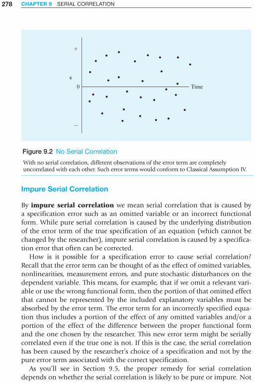
278 ChAPTER 9 Serial Correlation
Impure Serial Correlation
By impure serial correlation we mean serial correlation that is caused by a specification error such as an omitted variable or an incorrect functional form. While pure serial correlation is caused by the underlying distribution of the error term of the true specification of an equation (which cannot be changed by the researcher), impure serial correlation is caused by a specifica-tion error that often can be corrected.
How is it possible for a specification error to cause serial correlation? Recall that the error term can be thought of as the effect of omitted variables, nonlinearities, measurement errors, and pure stochastic disturbances on the dependent variable. This means, for example, that if we omit a relevant vari-able or use the wrong functional form, then the portion of that omitted effect that cannot be represented by the included explanatory variables must be absorbed by the error term. The error term for an incorrectly specified equa-tion thus includes a portion of the effect of any omitted variables and/or a portion of the effect of the difference between the proper functional form and the one chosen by the researcher. This new error term might be serially correlated even if the true one is not. If this is the case, the serial correlation has been caused by the researcher’s choice of a specification and not by the pure error term associated with the correct specification.
As you’ll see in Section 9.5, the proper remedy for serial correlation depends on whether the serial correlation is likely to be pure or impure. Not
2
1
0 Time
e
Figure 9.2 no Serial Correlation
With no serial correlation, different observations of the error term are completely uncorrelated with each other. Such error terms would conform to Classical Assumption IV.
M09_STUD2742_07_SE_C09.indd 278 1/9/16 2:04 PM

279 Pure verSuS imPure Serial Correlation
surprisingly, the best remedy for impure serial correlation is to attempt to find the omitted variable (or at least a good proxy) or the correct functional form for the equation. Both the bias and the impure serial correlation will disappear if the specification error is corrected. As a result, most econometri-cians try to make sure they have the best specification possible before they spend too much time worrying about pure serial correlation.
2
1
0 Time e
2
1
0 Time e
Figure 9.3 negative Serial Correlation
With negative first-order serial correlation, the current observation of the error term tends to have the opposite sign from the previous observation of the error term. In most time-series applications, negative serial correlation is much less likely than positive serial correlation.
M09_STUD2742_07_SE_C09.indd 279 1/9/16 2:04 PM

280 ChAPTER 9 Serial Correlation
To see how an omitted variable can cause the error term to be serially correlated, suppose that the true equation is:
Yt = β0 + β1X1t + β2X2t + et (9.3)
where et is a classical error term. As shown in Section 6.1, if X2 is accidentally omitted from the equation (or if data for X2 are unavailable), then:
Yt = β0 + β1X1t + e*t where e*t = β2X2t + et (9.4)
Thus, the error term in the omitted variable case is not the classical error term e. Instead, it’s also a function of one of the independent variables, X2. As a result, the new error term, e*, can be serially correlated even if the true error term e is not. In particular, the new error term e* will tend to exhibit detect-able serial correlation when:
1. X2 itself is serially correlated (this is quite likely in a time series) and
2. the size of e is small1 compared to the size of β2X2.
These tendencies hold even if there are a number of included and/or omitted variables. Therefore:
e*t = ρe*t - 1 + ut (9.5)
Another common kind of impure serial correlation is caused by an incor-rect functional form. Here, the choice of the wrong functional form can cause the error term to be serially correlated. Let’s suppose that the true equation is polynomial in nature:
Yt = β0 + β1X1t + β2X21t + et (9.6)
but that instead a linear regression is run:
Yt = α0 + α1X1t + e*t (9.7)
The new error term e* is now a function of the true error term e and of the differences between the linear and the polynomial functional forms. As can be seen in Figure 9.4, these differences often follow fairly autoregressive pat-terns. That is, positive differences tend to be followed by positive differences, and negative differences tend to be followed by negative differences. As a
1. If typical values of e are significantly larger in absolute size than β2X2, then even a serially correlated omitted variable (X2) will not change e* very much. In addition, recall that the omit-ted variable, X2, will cause bias in the estimate of β1, depending on the correlation between the two Xs. If βn1 is biased because of the omission of X2, then a portion of the β2X2 effect must have been absorbed by βn1 and will not end up in the residuals. As a result, tests for serial correlation based on those residuals may give incorrect readings. Such residuals may leave misleading clues as to possible specification errors.
M09_STUD2742_07_SE_C09.indd 280 1/9/16 2:04 PM

281 the ConSequenCeS of Serial Correlation
result, using a linear functional form when a nonlinear one is appropriate will usually result in positive impure serial correlation.
9.3 The Consequences of Serial Correlation
The consequences of serial correlation are quite different in nature from the consequences of the problems discussed so far in this text. Omitted variables, irrelevant variables, and multicollinearity all have fairly recognizable external
0
Y
X1
Y 5 b0 1 b1X1
0e
1
2
X1
Figure 9.4 incorrect functional form as a Source of impure Serial Correlation
The use of an incorrect functional form tends to group positive and negative residuals together, causing positive impure serial correlation.
M09_STUD2742_07_SE_C09.indd 281 1/9/16 2:04 PM

282 ChAPTER 9 Serial Correlation
symptoms. Each problem changes the estimated coefficients and standard errors in a particular way, and an examination of these changes (and the underlying theory) often provides enough information for the problem to be detected. As we shall see, serial correlation is more likely to have internal symptoms; it affects the estimated equation in a way that is not easily observ-able from an examination of just the results themselves.
The existence of serial correlation in the error term of an equation violates Classical Assumption IV, and the estimation of the equation with OLS has at least three consequences:2
2. If the regression includes a lagged dependent variable as an independent variable, then the problems worsen significantly. For more on this topic (called a dynamic model), see Chapter 12.
1. Pure serial correlation does not cause bias in the coefficient estimates.
2. Serial correlation causes OLS to no longer be the minimum variance estimator (of all the linear unbiased estimators).
3. Serial correlation causes the OLS estimates of the SE1βn 2s to be biased, leading to unreliable hypothesis testing.
1. Pure serial correlation does not cause bias in the coefficient estimates. If the error term is serially correlated, one of the assumptions of the Gauss–Markov Theorem is violated, but this violation does not cause the coef-ficient estimates to be biased. If the serial correlation is impure, however, bias may be introduced by the use of an incorrect specification.
This lack of bias does not necessarily mean that the OLS estimates of the coefficients of a serially correlated equation will be close to the true coefficient values. A single estimate observed in practice can come from a wide range of possible values. In addition, the standard errors of these estimates will typically be increased by the serial correlation. This increase will raise the probability that a βn will differ significantly from the true β value. What unbiased means in this case is that the distribu-tion of the βns is still centered around the true β.
2. Serial correlation causes OLS to no longer be the minimum variance estimator (of all the linear unbiased estimators). Although the violation of Classical Assumption IV causes no bias, it does affect the other main conclusion of the Gauss–Markov Theorem, that of minimum variance. In particular,
M09_STUD2742_07_SE_C09.indd 282 1/9/16 2:04 PM

283 the ConSequenCeS of Serial Correlation
we cannot prove that the distribution of the OLS βns is minimum vari-ance (among the linear unbiased estimators) when Assumption IV is violated.
The serially correlated error term causes the dependent variable to fluctuate in a way that the OLS estimation procedure sometimes at-tributes to the independent variables. Thus, OLS is more likely to mis-estimate the true β in the face of serial correlation. On balance, the βns are still unbiased because overestimates are just as likely as underesti-mates, but these errors increase the variance of the distribution of the estimates, increasing the amount that any given estimate is likely to dif-fer from the true β.
3. Serial correlation causes the OLS estimates of the SE(bn)s to be biased, leading to unreliable hypothesis testing. With serial correlation, the OLS formula for the standard error produces biased estimates of the SE(βn)s. Because the SE(βn) is a prime component in the t-statistic, these biased SE(βn)s cause biased t-scores and unreliable hypothesis testing in general. In essence, serial correlation causes OLS to produce incorrect SE(βn)s and t-scores! Not surprisingly, most econometricians therefore are very hesi-tant to put much faith in hypothesis tests that were conducted in the face of pure serial correlation.3
What sort of bias does serial correlation tend to cause? Typically, the bias in the estimate of SE(βn) is negative, meaning that OLS underes-timates the size of the standard errors of the coefficients. This comes about because serial correlation usually results in a pattern of observa-tions that allows a better fit than the actual (not serially correlated) observations would otherwise justify. This tendency of OLS to underes-timate the SE(βn) means that OLS typically overestimates the t-scores of the estimated coefficients, since:
t =1βn - βH0
2SE1βn 2 (9.8)
Thus the t-scores printed out by a typical software regression package in the face of serial correlation are likely to be too high. Similarly, confi-dence intervals for the coefficients will tend to be too narrow.
What will happen to hypothesis testing if OLS underestimates the SE(βn)s and therefore overestimates the t-scores? Well, the “too low” SE(βn) will cause
3. While our discussion here involves the t-test, the same conclusion of unreliability in the face of serial correlation applies to all other test statistics.
M09_STUD2742_07_SE_C09.indd 283 1/9/16 2:04 PM

284 ChAPTER 9 Serial Correlation
a “too high” t-score for a particular coefficient, and this will make it more likely that we will reject a null hypothesis (for example H0: β … 0) when it is in fact true. This increased chance of rejecting H0 means that we’re more likely to reject a true null hypothesis, so we’re more likely to make the mis-take of keeping an irrelevant variable in an equation because its coefficient’s t-score has been overestimated. In other words, hypothesis testing becomes unreliable when we have pure serial correlation.
9.4 The Detection of Serial Correlation
How can we detect serial correlation? While the first indication of serial cor-relation often occurs when we observe a pattern in the residuals similar to Figure 9.1, most econometricians rely on more formal tests like the Durbin–Watson test and the Lagrange Multiplier test.
The Durbin–Watson Test
The Durbin–Watson test is used to determine if there is first-order serial correlation in the error term of an equation by examining the residuals of a particular estimation of that equation.4 It’s important to use the Durbin–Watson test only when the assumptions that underlie its derivation are met:
1. The regression model includes an intercept term.
2. The serial correlation is first-order in nature:
et = ρet - 1 + ut (9.9)
where ρ is the autocorrelation coefficient and u is a classical (normally distributed) error term.
3. The regression model does not include a lagged dependent variable (discussed in Chapter 12) as an independent variable.5
The equation for the Durbin–Watson statistic for T observations is:
d = aT
21et - et - 122n aT
1e2
t (9.10)
4. J. Durbin and G. S. Watson, “Testing for Serial Correlation in Least-Squared Regression,” Biometrika, 1951, pp. 159–177.5. In such a circumstance, the Durbin–Watson test is biased toward 2.
M09_STUD2742_07_SE_C09.indd 284 1/9/16 2:04 PM

285 the DeteCtion of Serial Correlation
where the ets are the OLS residuals. Note that the numerator has one fewer observation than the denominator because an observation must be used to calculate et-1. The Durbin–Watson statistic equals 0 if there is extreme positive serial correlation, 2 if there is no serial correlation, and 4 if there is extreme negative serial correlation. To see this, let’s put appropriate residual values into Equation 9.10 for these three cases:
1. Extreme Positive Serial Correlation: d = 0 In this case, et = et-1, so 1et - et-12 = 0 and d = 0.
2. Extreme Negative Serial Correlation: d ≈ 4 In this case, et = -et-1, and 1et - et-12 = 12et2. Substituting into
Equation 9.10, we obtain d = g 12et22/g 1et22 and d ≈ 4.
3. No Serial Correlation: d ≈ 2 When there is no serial correlation, the mean of the distribution of d
is equal to 2.6 That is, if there is no serial correlation, d ≈ 2.
Using the Durbin–Watson Test
The Durbin–Watson test is unusual in two respects. First, econometricians almost never test the one-sided null hypothesis that there is negative serial correlation in the residuals because negative serial correlation, as mentioned previously, is quite difficult to explain theoretically in economic or business analysis. Its existence usually means that impure serial correlation has been caused by some specification error.
Second, the Durbin–Watson test is sometimes inconclusive. Whereas pre-viously explained decision rules always have had only “acceptance” regions and rejection regions, the Durbin–Watson test has a third possibility, called the inconclusive region. For reasons outlined in Section 9.5, we do not rec-ommend the application of a remedy for serial correlation if the Durbin–Watson test is inconclusive.7
6. To see this, multiply out the numerator of Equation 9.10, obtaining
d = c aT
2e2
t - 2aT
21etet-12 + aT
2e2
t-1 d n aT
1e2
t ≈ c aT
2e2
t + aT
2e2
t-1 d n aT
1e2
t ≈ 2 (9.11)
If there is no serial correlation, then et and et-1 are not related, and, on average, g 1etet-12 = 0.7. This inconclusive region is troubling, but the development of exact Durbin–Watson tests may eliminate this problem in the future. Some computer programs allow the user the option of cal-culating an exact Durbin–Watson probability (of first-order serial correlation). Alternatively, it’s worth noting that there is a growing trend toward the use of dU as a sole critical value. This trend runs counter to our view that if the Durbin–Watson test is inconclusive, then no remedial action should be taken except to search for a possible cause of impure serial correlation.
M09_STUD2742_07_SE_C09.indd 285 1/9/16 2:04 PM

286 Chapter 9 Serial Correlation
With these exceptions, the use of the Durbin–Watson test is quite similar to the use of the t-test. To test for positive serial correlation, the following steps are required:
1. Obtain the OLS residuals from the equation to be tested and calculate the d statistic by using Equation 9.10.
2. Determine the sample size and the number of explanatory variables and then consult Statistical Table B-4 in Appendix B to find the upper critical d value, dU, and the lower critical d value, dL, respectively. In-structions for the use of this table are also in that appendix.
3. Given the null hypothesis of no positive serial correlation and a one-sided alternative hypothesis:
H0: ρ … 0 (no positive serial correlation) HA: ρ 7 0 (positive serial correlation)
(9.12)
the appropriate decision rule is:
If d 6 dL Reject H0
If d 7 dU Do not reject H0
If dL … d … dU Inconclusive
In rare circumstances, perhaps first differenced equations, a two-sided Durbin–Watson test might be appropriate. In such a case, steps 1 and 2 are still used, but step 3 is now:
Given the null hypothesis of no serial correlation and a two-sided alternative hypothesis:
H0: ρ = 0 1no serial correlation2 HA: ρ ≠ 0 1serial correlation2
(9.13)
the appropriate decision rule is:
if d 6 dL Reject H0
if d 7 4 - dL Reject H0
if 4 - dU 7 d 7 dU Do not reject H0
otherwise Inconclusive
examples of the Use of the Durbin–Watson Statistic
Let’s work through some applications of the Durbin–Watson test. First, turn to Statistical Table B-4. Note that the upper and lower critical d values (dU and dL) depend on the number of explanatory variables (do not count the constant term), the sample size, and the level of significance of the test.
M09_STUD2742_07_SE_C09.indd 286 21/01/16 12:38 PM

287 the DeteCtion of Serial Correlation
Now let’s set up a one-sided 5-percent test for a regression with three explanatory variables and 25 observations. As can be seen from 5-percent table B-4, the critical values are dL = 1.12 and dU = 1.66. As a result, if the hypotheses are:
H0: ρ … 0 1no positive serial correlation2 HA: ρ 7 0 1positive serial correlation2
the appropriate decision rule is:
if d 6 1.12 Reject H0
if d 7 1.66 Do not reject H0
if 1.12 … d … 1.66 Inconclusive
A computed Durbin–Watson statistic of 1.78, for example, would indicate that there is no evidence of positive serial correlation, a value of 1.28 would be inconclusive, and a value of 0.60 would imply positive serial correlation. Figure 9.5 provides a graph of the “acceptance,” rejection, and inconclusive regions for this example.
For a real-world example, let’s look at a simple time-series model of the annual consumption of chicken in the United States. There are a variety of
0 20.60
dU 5 1.66dL 5 1.12 1.28 1.78
4
Inconclusive RegiondL , d , dU
Rejection Regiond , dL
“Acceptance” RegiondU , d
Positive SerialCorrelation
No Positive SerialCorrelation
Figure 9.5 an example of a one-Sided Durbin–Watson test
In a one-sided Durbin–Watson test for positive serial correlation, only values of d signif-icantly below 2 cause the null hypothesis of no positive serial correlation to be rejected. In this example, a d of 1.78 would indicate no positive serial correlation, a d of 0.60 would indicate positive serial correlation, and a d of 1.28 would be inconclusive.
M09_STUD2742_07_SE_C09.indd 287 1/9/16 2:04 PM

288 ChAPTER 9 Serial Correlation
variables that might make sense in such an equation, and at least three vari-ables seem obvious. We’d expect the demand for chicken to be a negative function of the price of chicken and a positive function of income and the price of a substitute (in this case, beef):
- + +Yt = β0 + β1PCt + β2PBt + β3YDt + et
where: Yt = per capita chicken consumption (in pounds) in year t PCt = the price of chicken (in cents per pound) in year t PBt = the price of beef (in cents per pound) in year t YDt = U.S. per capita disposable income (in hundreds of dollars)
in year tIf we collect data for these variables for the years 1974 through 2002, we
can estimate8 the following equation:
Ynt = 27.7 - 0.11PCt + 0.03PBt + 0.23YDt 10.032 10.022 10.012 t = -3.38 +1.86 +15.7
R 2 = .9904 N = 29 1annual 1974–20022
(9.14)
How does our estimated equation look? The overall fit of Equation 9.14 is excellent, and each of the individual regression coefficients is significantly dif-ferent from zero in the expected direction. The price of chicken does indeed have a significant negative effect (holding the price of beef and disposable income constant), and the price of beef and disposable income do indeed have positive effects (holding the other independent variables constant).
However, this is a time-series equation, so if there’s serial correlation, hypothesis testing will be unreliable, and one or more of these t-scores could be artificially high. We’d better run a Durbin–Watson test!
When we calculate a Durbin–Watson statistic for Equation 9.14,9 we get 0.99. Is that cause to be concerned about serial correlation? What would be the result of a one-sided 5-percent test of the null hypothesis of no positive serial correlation? Well, once we’ve got the Durbin–Watson statistic, the next
8. The data for this equation are in dataset CHICK9. As we’ll see in Chapter 14, estimating an equation for the demand for chicken without taking into account the simultaneously determined supply of chicken runs the risk of bias, particularly in the coefficient of the price of chicken.9. Luckily, you don’t actually need to calculate the Durbin–Watson statistic yourself. Some econometric software programs, including EViews, calculate the Durbin–Watson statistic auto-matically, while others, including Stata, allow you to do so quite simply. In Stata, for example, the command is estat dwatson.
M09_STUD2742_07_SE_C09.indd 288 1/9/16 2:04 PM

289 the DeteCtion of Serial Correlation
step is to consult Statistical Table B-4. In that table, with K (the number of explanatory variables10) equal to 3 and N (the number of observations) equal to 29, we find that the critical d values are dL = 1.20 and dU = 1.65. (It’s probably a good idea to check these d values yourself to make sure that you know how to look them up.)
The decision rule would thus be:
if d 6 1.20 Reject H0
if d 7 1.65 Do not reject H0
if 1.20 … d … 1.65 Inconclusive
Since 0.99 is less than the critical lower limit of the d statistic, we would reject the null hypothesis of no positive serial correlation, and we would have to decide how to cope with that serial correlation.
The Lagrange Multiplier (LM) test
Unfortunately, the Durbin–Watson test has a number of limitations. As men-tioned, it can be used only when the serial correlation is first-order, when a constant is included in the equation, and when the equation doesn’t include a lagged dependent variable. The Durbin–Watson test’s inconclusive region also is a drawback, particularly since the size of the inconclusive region increases as the number of independent variables increases.
A popular alternative to the Durbin–Watson test is the Lagrange Multi-plier (LM) test, which checks for serial correlation by analyzing how well the lagged residuals explain the residual of the original equation in an equa-tion that also includes all the explanatory variables of the original model. If the lagged residuals are significant in explaining this time’s residuals (as shown by the chi-square test), then we can reject the null hypothesis of no serial correlation.11 The LM serial correlation test is just one application of a
10. Be careful! While we define K as the number of explanatory variables, some other sources, including Stata and the Stanford University Durbin–Watson tables, define K as the number of coefficients (which is equivalent to K + 1 in our notation). As long as you’re aware of this dif-ference, it won’t cause you any problems. Incidentally, the Stanford tables, which are online at http://web.stanford.edu/~clint/bench/dwcrit.htm, have many more observations than can be printed in a textbook, so they’re quite useful if you have a large sample.11. The Lagrange Multiplier test for serial correlation is sometimes referred to as the Breusch–Godfrey test, which is why the Stata command for this test is estat bgodfrey, lag (1). Note that if we’re testing for first-order serial correlation, we need to specify that the lag equals 1. If we are concerned with second-order serial correlation, then the lag would equal 2, etc.
M09_STUD2742_07_SE_C09.indd 289 1/9/16 2:04 PM
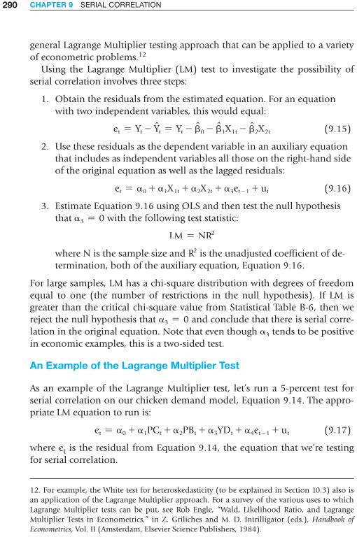
290 ChAPTER 9 Serial Correlation
general Lagrange Multiplier testing approach that can be applied to a variety of econometric problems.12
Using the Lagrange Multiplier (LM) test to investigate the possibility of serial correlation involves three steps:
1. Obtain the residuals from the estimated equation. For an equation with two independent variables, this would equal:
et = Yt - Ynt = Yt - βn 0 - βn 1X1t - βn 2X2t (9.15)
2. Use these residuals as the dependent variable in an auxiliary equation that includes as independent variables all those on the right-hand side of the original equation as well as the lagged residuals:
et = α0 + α1X1t + α2X2t + α3et - 1 + ut (9.16)
3. Estimate Equation 9.16 using OLS and then test the null hypothesis that α3 = 0 with the following test statistic:
LM = NR2
where N is the sample size and R2 is the unadjusted coefficient of de-termination, both of the auxiliary equation, Equation 9.16.
For large samples, LM has a chi-square distribution with degrees of freedom equal to one (the number of restrictions in the null hypothesis). If LM is greater than the critical chi-square value from Statistical Table B-6, then we reject the null hypothesis that α3 = 0 and conclude that there is serial corre-lation in the original equation. Note that even though α3 tends to be positive in economic examples, this is a two-sided test.
An Example of the Lagrange Multiplier Test
As an example of the Lagrange Multiplier test, let’s run a 5-percent test for serial correlation on our chicken demand model, Equation 9.14. The appro-priate LM equation to run is:
et = α0 + α1PCt + α2PBt + α3YDt + α4et - 1 + ut (9.17)
where et is the residual from Equation 9.14, the equation that we’re testing for serial correlation.
12. For example, the White test for heteroskedasticity (to be explained in Section 10.3) also is an application of the Lagrange Multiplier approach. For a survey of the various uses to which Lagrange Multiplier tests can be put, see Rob Engle, “Wald, Likelihood Ratio, and Lagrange Multiplier Tests in Econometrics,” in Z. Griliches and M. D. Intrilligator (eds.), Handbook of Econometrics, Vol. II (Amsterdam, Elsevier Science Publishers, 1984).
M09_STUD2742_07_SE_C09.indd 290 1/9/16 2:04 PM

291 remeDieS for Serial Correlation
Since there are three independent variables, the null hypothesis becomes H0: α4 = 0. If we estimate Equation 9.17, we get an R2 of .291. Since the sample size is 29, this means that:
LM = NR2 = 8.439
The decision rule is to reject the null hypothesis if NR2 is greater than the crit-ical chi-square value with 1 degree of freedom, so the next step is to consult Table B-6 and look up the critical value. As you can see if you take a look at Table B-6, the 5-percent chi-square critical value with 1 degree of freedom is 3.84. Since 8.439 7 3.84, we can reject the null hypothesis and conclude that we have serial correlation in the chicken demand model. This is a two-sided test, but it confirms the result of our one-sided Durbin–Watson test. It seems clear that the chicken demand equation has serial correlation!
9.5 Remedies for Serial Correlation
Suppose that the Durbin–Watson or LM test detects serial correlation in the residuals of your equation. Is there a remedy? Some students suggest reorder-ing the observations of Y and the Xs to avoid serial correlation. They think that if this time’s error term appears to be affected by last time’s error term, why not reorder the data randomly to get rid of the problem? The answer is that the reordering of the data does not get rid of the serial correlation; it just makes the problem harder to detect. If e2 = f1e12 and we reorder the data, then the error term observations are still related to each other, but they now no longer follow each other, and it becomes almost impossible to discover the serial correlation. Interestingly, reordering the data changes the Durbin–Watson statistic but does not change the estimates of the coefficients or their standard errors at all.13
13. This can be proven mathematically, but it is usually more instructive to estimate a regres-sion yourself, change the order of the observations, and then reestimate the regression. See Exercise 3 at the end of the chapter.
The place to start in correcting a serial correlation problem is to look carefully at the specification of the equation for possible errors that might be causing impure serial correlation. Is the functional form cor-rect? Are you sure that there are no omitted variables? Only after the specification of the equation has been reviewed carefully should the pos-sibility of an adjustment for pure serial correlation be considered.
M09_STUD2742_07_SE_C09.indd 291 1/9/16 2:04 PM
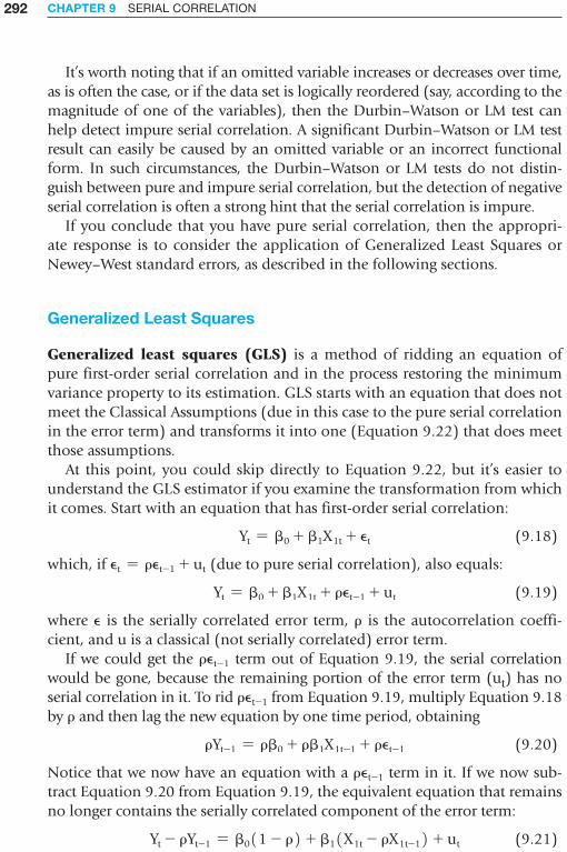
292 ChAPTER 9 Serial Correlation
It’s worth noting that if an omitted variable increases or decreases over time, as is often the case, or if the data set is logically reordered (say, according to the magnitude of one of the variables), then the Durbin–Watson or LM test can help detect impure serial correlation. A significant Durbin–Watson or LM test result can easily be caused by an omitted variable or an incorrect functional form. In such circumstances, the Durbin–Watson or LM tests do not distin-guish between pure and impure serial correlation, but the detection of negative serial correlation is often a strong hint that the serial correlation is impure.
If you conclude that you have pure serial correlation, then the appropri-ate response is to consider the application of Generalized Least Squares or Newey–West standard errors, as described in the following sections.
Generalized Least Squares
Generalized least squares (GLS) is a method of ridding an equation of pure first-order serial correlation and in the process restoring the minimum variance property to its estimation. GLS starts with an equation that does not meet the Classical Assumptions (due in this case to the pure serial correlation in the error term) and transforms it into one (Equation 9.22) that does meet those assumptions.
At this point, you could skip directly to Equation 9.22, but it’s easier to understand the GLS estimator if you examine the transformation from which it comes. Start with an equation that has first-order serial correlation:
Yt = β0 + β1X1t + et (9.18)
which, if et = ρet-1 + ut (due to pure serial correlation), also equals:
Yt = β0 + β1X1t + ρet-1 + ut (9.19)
where e is the serially correlated error term, ρ is the autocorrelation coeffi-cient, and u is a classical (not serially correlated) error term.
If we could get the ρet-1 term out of Equation 9.19, the serial correlation would be gone, because the remaining portion of the error term (ut) has no serial correlation in it. To rid ρet-1 from Equation 9.19, multiply Equation 9.18 by ρ and then lag the new equation by one time period, obtaining
ρYt-1 = ρβ0 + ρβ1X1t-1 + ρet-1 (9.20)
Notice that we now have an equation with a ρet-1 term in it. If we now sub-tract Equation 9.20 from Equation 9.19, the equivalent equation that remains no longer contains the serially correlated component of the error term:
Yt - ρYt-1 = β011 - ρ2 + β11X1t - ρX1t-12 + ut (9.21)
M09_STUD2742_07_SE_C09.indd 292 1/9/16 2:04 PM

293 remedieS for Serial Correlation
Equation 9.21 can be rewritten as:
Y t* = β0* + β1X1t* + ut (9.22)
where: Y*t = Yt - ρYt - 1 (9.23) X*1t = X1t - ρX1t - 1
β*0 = β0 - ρβ0
Equation 9.22 is called a Generalized Least Squares (or “quasi-differenced”) version of Equation 9.19. Notice that:
1. The error term is not serially correlated. As a result, OLS estimation of Equation 9.22 will be minimum variance. (This is true if we know ρ or if we accurately estimate ρ.)
2. The slope coefficient β1 is the same as the slope coefficient of the origi-nal serially correlated equation, Equation 9.19. Thus coefficients esti-mated with GLS have the same meaning as those estimated with OLS.
3. The dependent variable has changed compared to that in Equation 9.19. This means that the GLS R
2 is not necessarily comparable to the OLS R
2.
Unfortunately we can’t use OLS to estimate a Generalized Least Squares model because GLS equations are inherently nonlinear in the coefficients. To see why, take a look at Equation 9.21. We need to estimate values not only for β0 and β1 but also for ρ, and ρ is multiplied by β0 and β1 (which you can see if you multiply out the right-hand side of the equation). Since OLS requires that the equation be linear in the coefficients, we need a different estimation procedure.
Luckily, there are a number of techniques that can be used to estimate GLS equations. While the best-known of these is the Cochrane–Orcutt method,14 our recommendation is to use a slightly different approach, the Prais–Winsten method. The Prais–Winsten method15 is a two–step itera-tive technique that rids an equation of serial correlation by first producing
14. D. Cochrane and G. H. Orcutt, “Application of Least Squares Regression to Relationships Con-taining Autocorrelated Error Terms,” Journal of the American Statistical Association, 1949, pp. 32–61.15. S. J. Prais and C. B. Winsten, “Trend Estimators and Serial Correlation,” Cowles Commis-sion Discussion Paper No. 383 (1954) Chicago. The Prais–Winsten method (sometimes called Yule–Walker) is very similar to Cochrane–Orcutt, but the Prais–Winsten estimate of ρ is more accurate because it uses the first observation in Step 1 while Cochrane–Orcutt does not. For more, see Masahito Kobayashi, “Comparison of Efficiencies of Several Estimators for Linear Regressions with Autocorrelated Errors,” Journal of the American Statistical Association, 1985, pp. 951–953.
M09_STUD2742_07_SE_C09.indd 293 21/01/16 12:38 PM

294 ChAPTER 9 Serial Correlation
an estimate of ρ and then estimating the GLS equation using that ρn. The two steps are:
1. Estimate ρ by running a regression based on the residuals of the equa-tion suspected of having serial correlation:
et = ρet - 1 + ut (9.24)
where the ets are the OLS residuals from the equation suspected of hav-ing pure serial correlation and ut is a classical (non-serially-correlated) error term.
2. Use this ρn to estimate the GLS equation by substituting ρn into Equa-tion 9.21 and using OLS to estimate Equation 9.21 with the adjusted data.
These two steps are repeated (iterated) until further improvement results in little change in ρn. Once ρn has converged (usually in just a few iterations), the last estimate of step 2 is used as the final estimate of Equation 9.21.
Unfortunately, all methods of estimating GLS equations use iterative non-linear regression techniques that are well beyond the scope of this text. As a result, most researchers rely on their econometric software packages to estimate their GLS equations for them. In Stata, for example, the Prais–Winsten method can be run using the command prais followed by a listing of the dependent and independent variables.16
Let’s apply Generalized Least Squares, using the Prais–Winsten method, to the chicken demand example that was found to have serial correlation in the previous section. Recall that we estimated the per capita demand for chicken as a function of the price of chicken, the price of beef, and disposable income:
Ynt = 27.7 - 0.11PCt + 0.03PBt + 0.23YDt
10.032 10.022 10.012 t = -3.38 + 1.86 +15.7
R
2 = .9904 N = 29 DW = 0.99
(9.14)
Note that we have added the Durbin–Watson statistic to the documenta-tion with the notation DW. All future time-series results will include the DW statistic, but cross-sectional documentation of the DW is not required unless the observations are ordered in some meaningful manner (like smallest to largest or youngest to oldest).
16. In Stata, the command to apply GLS (using Prais–Winsten) to Equation 9.14 thus would be prais Y PC PB YD. In EViews, the easiest way to estimate a GLS equation is to add AR(1) to the equation as an independent variable, as in: LS Y C PC PB YD AR(1). The result is a GLS estimate where ρn will appear as the estimated coefficient of the variable AR(1).
M09_STUD2742_07_SE_C09.indd 294 1/9/16 2:04 PM

295 remeDieS for Serial Correlation
If we reestimate Equation 9.14 with the Prais–Winsten approach to GLS, we obtain:
Yt = 28.5 - 0.08PCt + 0.016PBt + 0.24YDt
10.042 10.0212 10.022 t = - 2.13 + 0.74 +13.12
R
2 = .963 N = 29 ρn = 0.56
(9.25)
Let’s compare Equations 9.14 and 9.25. Note that the ρn used in Equation 9.25 is 0.56. This means that Y was actually run as Y* = Yt - 0.56Yt - 1, PC as PC* = PCt - 0.56PCt - 1, etc. Second, ρn replaces DW in the documentation of GLS estimates in part because the DW of Equation 9.25 isn’t strictly compa-rable to non-GLS DWs (it is biased toward 2).
Generalized Least Squares estimates, no matter how they are produced, have at least two problems. First, even though serial correlation causes no bias in the estimates of the βns, the GLS estimates usually are different from the OLS ones. For example, note that all three slope coefficients change as we move from OLS in Equation 9.14 to GLS in Equation 9.25. This isn’t surprising, since different estimates can have different values even though their expected values are the same. The second problem is more impor-tant, however. It turns out that GLS works well if ρn is close to the actual ρ, but the GLS ρn is biased in small samples. If ρn is biased, then the biased ρn introduces bias into the GLS estimates of the βns. Luckily, there is a remedy for serial correlation that helps avoid both of these problems: Newey–West standard errors.
Newey–West Standard Errors
Not all corrections for pure serial correlation involve Generalized Least Squares. Newey–West standard errors are SE(βn)s that take account of serial cor-relation without changing the βns themselves in any way.17 The logic behind Newey–West standard errors is powerful. If serial correlation does not cause bias in the βns but does impact the standard errors, then it makes sense to adjust the estimated equation in a way that changes the SE(βn)s but not the βns.
17. W. K. Newey and K. D. West, “A Simple, Positive Semi-Definite Heteroskedasticity and Autocorrelation Consistent Covariance Matrix,” Econometrica, 1987, pp. 703–708. Newey–West standard errors are similar to HC standard errors (or White standard errors), to be discussed in Section 10.4.
M09_STUD2742_07_SE_C09.indd 295 1/9/16 2:04 PM

296 ChAPTER 9 Serial Correlation
Thus Newey–West standard errors have been calculated specifically to avoid the consequences of pure first-order serial correlation. The Newey–West procedure yields an estimator of the standard errors that, while they are biased, is generally more accurate than uncorrected standard errors for large samples (greater than 100) in the face of serial correlation. As a result, Newey–West standard errors can be used for t-tests and other hypothesis tests in most samples without the errors of inference potentially caused by serial correlation. Typically, Newey–West SE(βn)s are larger than OLS SE(βn)s, thus producing lower t-scores and decreasing the probability that a given esti-mated coefficient will be significantly different from zero.
To see how Newey–West standard errors work, let’s apply them to the same serially correlated chicken demand equation to which we applied GLS in Equation 9.14. If we use Newey–West standard errors in the estimation of Equation 9.14, we get:
Ynt = 27.7 - 0.11PCt + 0.03PBt + 0.23YDt (9.26) 10.032 10.022 10.012 t = -3.30 + 2.12 +19.2
R
2 = .9904 N = 29
Let’s compare Equations 9.14 and 9.26. First of all, the βns are identical in Equations 9.14 and 9.26. This is because Newey–West standard errors do not change the OLS βns. Second, while we can’t observe the change because of rounding, the Newey–West standard errors must be different from the OLS standard errors because the t-scores have changed even though the esti-mated coefficients are identical. However, two of the Newey–West SE(βn)s are slightly lower than the OLS SE(βn)s, which is a surprise even in a small sample like this one. Such a result indicates that there may well be an omitted vari-able or nonstationarity (to be discussed in Chapter 12) in this equation.
9.6 Summary
1. Serial correlation, or autocorrelation, is the violation of Classical As-sumption IV that the observations of the error term are uncorrelated with each other. Usually, econometricians focus on first-order serial correlation, in which the current observation of the error term is as-sumed to be a function of the previous observation of the error term and a not-serially-correlated error term (u):
et = ρet - 1 + ut - 1 6 ρ 6 1
where ρ is “rho,” the autocorrelation coefficient.
M09_STUD2742_07_SE_C09.indd 296 1/9/16 2:04 PM

297ExErcisEs
2. Pure serial correlation is serial correlation that is a function of the error term of the correctly specified regression equation. Impure serial correlation is caused by specification errors such as an omitted vari-able or an incorrect functional form. While impure serial correlation can be positive 10 6 ρ 6 +12 or negative 1-1 6 ρ 6 02 pure serial correlation in economics or business situations is almost always posi-tive (unless first differences are involved).
3. The major consequence of serial correlation is bias in the OLS SE (βn)s, causing unreliable hypothesis testing. Pure serial correlation does not cause bias in the estimates of the βs.
4. A commonly used method of detecting first-order serial correlation is the Durbin–Watson test, which uses the residuals of an estimated regression to test the possibility of serial correlation in the error term. An often-preferred alternative is the Lagrange Multiplier (LM) test, which is far more general than the Durbin–Watson test.
5. The first step in ridding an equation of serial correlation is to check for possible specification errors. Only once the possibility of impure serial correlation has been reduced to a minimum should remedies for pure serial correlation be considered.
6. Generalized Least Squares (GLS) is a method of transforming an equation to rid it of pure first-order serial correlation. The use of GLS requires the estimation of ρ.
7. Newey–West standard errors are an alternative remedy for serial cor-relation that adjusts the OLS estimates of the SE(βn)s to take account of the serial correlation without changing the βns.
ExErcisEs
(The answers to the even-numbered exercises are in Appendix A.)
1. Write the meaning of each of the following terms without referring to the book (or your notes), and compare your definition with the ver-sion in the text for each.a. Durbin–Watson test (p. 284)b. first-order auto correlation coefficient (p. 275)c. first-order serial correlation (p. 275)d. Generalized Least Squares (GLS) (p. 292)e. impure serial correlation (p. 278)
M09_STUD2742_07_SE_C09.indd 297 02/02/16 1:55 PM

298 Chapter 9 Serial Correlation
f. Lagrange Multiplier (LM) test (p. 289)g. negative serial correlation (p. 276)h. Newey–West standard errors (p. 295)i. positive serial correlation (p. 276)j. Prais–Winsten method (p. 293)k. pure serial correlation (p. 275)
2. Consider the following equation for U.S. per capita consumption of beef:
CBt = - 330.3 + 49.1lnYt - 0.34PBt + 0.33PRPt - 15.4Dt
17.42 10.132 10.122 14.12 t = 6.6 - 2.6 2.7 - 3.7 R
2 = .700 N = 28 DW = 0.94
(9.27)
where: CBt = the annual per capita pounds of beef consumed in the United States in year t
ln Yt = the log of per capita disposable real income in the U.S. in year t
PBt = average annualized real wholesale price of beef in year t (in cents per pound)
PRPt = average annualized real wholesale price of pork in year t (in cents per pound)
Dt = a dummy variable equal to 1 for years in which there was a “health scare” about the dangers of red meat, 0 otherwise
a. Develop and test your own hypotheses with respect to the indi-vidual estimated slope coefficients.
b. Test for serial correlation in Equation 9.27 using the Durbin–Watson test at the 5-percent level.
c. What econometric problem(s) (if any) does Equation 9.27 appear to have? What remedy would you suggest?
d. You take your own advice and apply GLS to Equation 9.27, obtaining:
CBt = -193.3 + 35.2ln Yt - 0.38PBt + 0.10PRPt - 5.7Dt
114.12 10.102 10.092 13.92 t = 2.5 -3.7 1.1 -1.5 R
2 = .857 N = 28 ρn = 0.82
(9.28)
Compare Equations 9.27 and 9.28. Which do you prefer? Why?
3. Recall from Section 9.5 that switching the order of a data set will not change its coefficient estimates. A revised order will change the Durbin–Watson statistic, however. To see both these points, run
99
M09_STUD2742_07_SE_C09.indd 298 21/01/16 12:38 PM

299exerCiSeS
regressions 1HS = β0 + β1P + e2 and compare the coefficient esti-mates and DW statistics for this data set:
Year Housing Starts Population
1 9090 2200
2 8942 2222
3 9755 2244
4 10327 2289
5 10513 2290
in the following three orders (in terms of year):a. 1, 2, 3, 4, 5b. 5, 4, 3, 2, 1c. 2, 4, 3, 5, 1
4. Suppose that the data in a time-series study were entered in reverse chronological order. Would this change in any way the testing or adjusting for serial correlation? How? In particular:a. What happens to the Durbin–Watson statistic’s ability to detect
serial correlation if the order is reversed?b. What happens to the GLS method’s ability to adjust for serial cor-
relation if the order is reversed?c. What is the intuitive economic explanation of reverse serial cor-
relation?
5. Your friend is just finishing a study of attendance at Los Angeles Laker regular-season home basketball games when she hears that you’ve read a chapter on serial correlation and asks your advice. Before run-ning the equation on last season’s data, she “reviewed the literature” by interviewing a number of basketball fans. She found out that fans like to watch winning teams. In addition, she learned that while some fans like to watch games throughout the season, others are most interested in games played late in the season. Her estimated equation (standard errors in parentheses) was:
An t = 14123 + 20L t + 2600Pt + 900Wt
15002 110002 13002 DW = 0.85 N = 40 R 2 = .46
where: At = the attendance at game t Lt = the winning percentage (games won divided by games
played) of the Lakers before game t
M09_STUD2742_07_SE_C09.indd 299 1/9/16 2:04 PM

300 ChAPTER 9 Serial Correlation
Pt = the winning percentage before game t of the Lakers’ opponent in that game
Wt = a dummy variable equal to 1 if game t was on Friday, Satur-day, or Sunday, 0 otherwise
a. Test for serial correlation using the Durbin–Watson test at the 5-percent level.
b. Make and test appropriate hypotheses about the slope coefficients at the 1-percent level.
c. Compare the size and significance of the estimated coefficient of L with that for P. Is this difference surprising? Is L an irrelevant vari-able? Explain your answer.
d. If serial correlation exists, would you expect it to be pure or impure serial correlation? Why?
e. Your friend omitted the first game of the year from the sample be-cause the first game is always a sellout and because neither team had a winning percentage yet. Was this a good decision?
6. In a 1988 article, Josef Brada and Ronald Graves built an interest-ing model of defense spending in the Soviet Union just before the breakup of that nation.18 The authors felt sure that Soviet defense spending was a function of U.S. defense spending and Soviet GNP but were less sure about whether defense spending also was a function of the ratio of Soviet nuclear warheads to U.S. nuclear warheads. Using a double-log functional form, the authors estimated a number of alter-native specifications, including (standard errors in parentheses):
lnSDHt = - 1.99 + 0.056lnUSDt + 0.969lnSYt + 0.057lnSPt
10.0742 10.0652 10.0322 t = 0.76 14.98 1.80
N = 25 1annual 1960–19842 R
2 = .979 DW = 0.49
(9.29)
lnSDHt = - 2.88 + 0.105lnUSDt + 1.066lnSYt
10.0732 10.0382 t = 1.44 28.09
N = 25 1annual 1960–19842 R
2 = .977 DW = 0.43
(9.30)
®
®
18. Josef C. Brada and Ronald L. Graves, “The Slowdown in Soviet Defense Expenditures,” Southern Economic Journal, Vol. 54, No. 4, pp. 969–984. In addition to the variables used in this exercise, Brada and Graves also provide data for SFPt, the rate of Soviet factor productivity in year t, which we include in Table 9.1.
M09_STUD2742_07_SE_C09.indd 300 1/9/16 2:04 PM
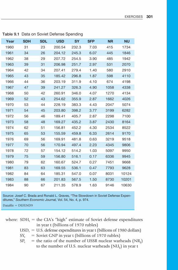
301exerCiSeS
where: SDHt = the CIA’s “high” estimate of Soviet defense expenditures in year t (billions of 1970 rubles)
USDt = U.S. defense expenditures in year t (billions of 1980 dollars) SYt = Soviet GNP in year t (billions of 1970 rubles) SPt = the ratio of the number of USSR nuclear warheads (NRt)
to the number of U.S. nuclear warheads (NUt) in year t
Table 9.1 Data on Soviet Defense Spending
Year SDh SDL USD SY SFP NR NU
1960 31 23 200.54 232.3 7.03 415 1734
1961 34 26 204.12 245.3 6.07 445 1846
1962 38 29 207.72 254.5 3.90 485 1942
1963 39 31 206.98 251.7 2.97 531 2070
1964 42 34 207.41 279.4 1.40 580 2910
1965 43 35 185.42 296.8 1.87 598 4110
1966 44 36 203.19 311.9 4.10 674 4198
1967 47 39 241.27 326.3 4.90 1058 4338
1968 50 42 260.91 346.0 4.07 1270 4134
1969 52 43 254.62 355.9 2.87 1662 4026
1970 53 44 228.19 383.3 4.43 2047 5074
1971 54 45 203.80 398.2 3.77 3199 6282
1972 56 46 189.41 405.7 2.87 2298 7100
1973 58 48 169.27 435.2 3.87 2430 8164
1974 62 51 156.81 452.2 4.30 2534 8522
1975 65 53 155.59 459.8 6.33 2614 9170
1976 69 56 169.91 481.8 0.63 3219 9518
1977 70 56 170.94 497.4 2.23 4345 9806
1978 72 57 154.12 514.2 1.03 5097 9950
1979 75 59 156.80 516.1 0.17 6336 9945
1980 79 62 160.67 524.7 0.27 7451 9668
1981 83 63 169.55 536.1 0.47 7793 9628
1982 84 64 185.31 547.0 0.07 8031 10124
1983 88 66 201.83 567.5 1.50 8730 10201
1984 90 67 211.35 578.9 1.63 9146 10630
Source: Josef C. Brada and ronald l. Graves, “the Slowdown in Soviet Defense expen-ditures,” Southern Economic Journal, vol. 54, no. 4, p. 974.
Datafile 5 DEFEND9
M09_STUD2742_07_SE_C09.indd 301 1/9/16 2:04 PM
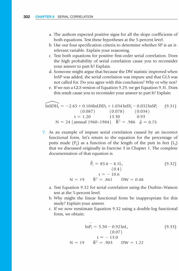
302 ChAPTER 9 Serial Correlation
a. The authors expected positive signs for all the slope coefficients of both equations. Test these hypotheses at the 5-percent level.
b. Use our four specification criteria to determine whether SP is an ir-relevant variable. Explain your reasoning.
c. Test both equations for positive first-order serial correlation. Does the high probability of serial correlation cause you to reconsider your answer to part b? Explain.
d. Someone might argue that because the DW statistic improved when lnSP was added, the serial correlation was impure and that GLS was not called for. Do you agree with this conclusion? Why or why not?
e. If we run a GLS version of Equation 9.29, we get Equation 9.31. Does this result cause you to reconsider your answer to part b? Explain
lnSDHt = -2.65 + 0.104lnUSDt + 1.034 lnSYt - 0.032 lnSPt
10.0872 10.0782 10.0342 t = 1.20 13.30 0.93
N = 24 1annual 1960–19842 R
2 = .986 ρn = 0.75
(9.31)
7. As an example of impure serial correlation caused by an incorrect functional form, let’s return to the equation for the percentage of putts made (Pi) as a function of the length of the putt in feet (Li) that we discussed originally in Exercise 3 in Chapter 1. The complete documentation of that equation is
Pni = 83.6 - 4.1Li
10.42 t = - 10.6
N = 19 R
2 = .861 DW = 0.48
(9.32)
a. Test Equation 9.32 for serial correlation using the Durbin–Watson test at the 5-percent level.
b. Why might the linear functional form be inappropriate for this study? Explain your answer.
c. If we now reestimate Equation 9.32 using a double-log functional form, we obtain:
lnPi = 5.50 - 0.92 lnLi
10.072 t = - 13.0
N = 19 R
2 = .903 DW = 1.22
(9.33)
®
h
M09_STUD2742_07_SE_C09.indd 302 1/9/16 2:04 PM

303appendix: eConometriC lab #5
Test Equation 9.33 for serial correlation using the Durbin–Watson test at the 5-percent level.
d. Compare Equations 9.32 and 9.33. Which equation do you prefer? Why?
9.7 appendix: econometric Lab #5
In this lab, you’ll expand on Econometric Lab #2 by estimating an aggregate consumption function for the U.S. economy for the period 1945–2006, test-ing your equation for serial correlation, and, if appropriate, taking corrective action.19
Step 1: State the Variables and the expected Signs of the Coefficients
As in Econometric Lab #2, our goal is to model U.S. aggregate consumption as a function of disposable personal income and the real interest rate. Once again, the data are from the St. Louis Federal Reserve FRED database and the Economic Report of the President. Descriptions of the variables are in Table 9.2, along with the hypothesized signs for the coefficients, and the dataset itself is on the text’s website as CONS9.
Table 9.2 Variable definitionsVariable Description expected sign
cont real personal consumption expenditures in year t, in billions of 2009 dollars
na
dpit real disposable personal income in year t, in billions of 2009 dollars
1
aaat the real interest rate on aaa corporate bonds in year t
2
yeart Year t na
19. Econometric Lab #2 used a sample for the period 1945–2014, but we end Lab #5’s sample in 2006 to avoid the (admittedly interesting) complications introduced by the Great Recession.
M09_STUD2742_07_SE_C09.indd 303 21/01/16 12:38 PM

304 ChAPTER 9 Serial Correlation
Step 2: Estimate the Aggregate Consumption Function
Now estimate the consumption function, using disposable personal income and the real interest rate as the independent variables.20
Step 3: Examine the Residuals
Generate the residuals from the regression in Step 2 (naming them “e”) and plot them as a line graph against yeart (with yeart on the x-axis). Does the plot look entirely random? Explain.
Step 4: Run the Durbin–Watson Test
Conduct a Durbin–Watson test for positive serial correlation.
a. Carefully write down the null and alternative hypotheses.
b. Run a Durbin–Watson test for positive serial correlation at the 5-percent level. What are the upper and lower critical values in this case? What can you conclude? Explain.
Step 5: Run the Lagrange Multiplier Serial Correlation Test
Let’s see if our Durbin–Watson results can be confirmed with the Lagrange Multiplier test.
a. Are the null and alternative hypotheses for the Lagrange Multiplier test the same as for the Durbin–Watson test? Why or why not?
b. Conduct a Lagrange Multiplier test for serial correlation at the 5-percent level. What can you conclude? Explain.
Step 6: Estimate the Model with Generalized Least Squares
a. If you encountered serial correlation in either of the previous steps, re-estimate our aggregate consumption model using Generalized Least Squares.
20. If you’re using Stata, be sure to tell Stata that this is a time series and that yeart is the time variable.
M09_STUD2742_07_SE_C09.indd 304 1/9/16 2:04 PM

305appendix: eConometriC lab #5
b. Are the GLS coefficients and t-statistics the same as the OLS coeffi-cients and t-statistics? Explain.
c. After the GLS transformation, does serial correlation still appear to exist? Support your answer.
Step 7: Calculate Newey-West Standard errors
a. If you ran a GLS model in Step 6, now estimate the aggregate con-sumption model using the Newey–West method with a lag of 1.
b. After the Newey–West calculation, are the coefficients the same as the OLS coefficients? Explain.
c. Why are the Newey–West t-statistics different from the OLS t-statistics? Which do you prefer? Why?
M09_STUD2742_07_SE_C09.indd 305 21/01/16 12:38 PM

Time-Series Models
12.1 Distributed Lag Models
12.2 Dynamic Models
12.3 Serial Correlation and Dynamic Models
12.4 Granger Causality
12.5 Spurious Correlation and Nonstationarity
12.6 Summary and Exercises
Chapter 12
The purpose of this chapter is to provide an introduction to a number of interesting models that have been designed to cope with and take advantage of the special properties of time-series data. Working with time-series data often causes complications that simply can’t happen with cross-sectional data. Most of these complications involve the order of the observations because order matters quite a bit in time-series data but doesn’t matter much (if at all) in cross-sectional data.
The most important of the topics concerns a class of dynamic models in which a lagged value of the dependent variable appears on the right-hand side of the equation. As you will see, the presence of a lagged dependent vari-able on the right-hand side of the equation implies that the impact of the independent variables can be spread out over a number of time periods.
Why would you want to distribute the impact of an independent variable over a number of time periods? To see why, consider the impact of advertis-ing on sales. Most analysts believe that people remember advertising for more than one time period, so advertising affects sales in the future as well as in the current time period. As a result, models of sales should include current and lagged values of advertising, thus distributing the impact of advertising over a number of different lags.
While this chapter focuses on such dynamic models, you’ll also learn about models in which different numbers of lags appear and we’ll investigate
364
M12_STUD2742_07_SE_C12.indd 364 1/9/16 2:19 PM

365 DistributeD Lag MoDeLs
how the presence of these lags affects our estimators. The chapter concludes with a brief introduction to a topic called nonstationarity. If variables have significant changes in basic properties (like their mean or variance) over time, they are said to be nonstationary, and it turns out that nonstationary variables have the potential to inflate t-scores and measures of overall fit in an equation.
12.1 Distributed Lag Models
As described in Section 7.3, lagged independent variables can be used when-ever you expect X to affect Y after a period of time. For example, if the under-lying theory suggests that X1 affects Y with a one-time-period lag (but X2 has an instantaneous impact on Y), we use equations like:
Yt = β0 + β1X1t - 1 + β2X2t + et (7.14)
Such lags are called simple lags, and the estimation of β1 with OLS is no more difficult than the estimation of the coefficients of nonlagged equa-tions, except for possible impure serial correlation if the lag is misspeci-fied. Remember, however, that the coefficients of such equations should be interpreted carefully. For example, β2 in Equation 7.14 measures the effect of a one-unit increase in this time’s X2 on this time’s Y holding last time’s X1 constant.
A case that’s more complicated than this one-period lag occurs when the impact of an independent variable is expected to be spread out over a number of time periods. Suppose, for example, that we’re interested in studying the impact of a change in the money supply on GDP. Theoretical and empirical studies have provided evidence that, because of rigidities in the marketplace, it takes time for the economy to react completely to a change in the money supply. If it takes two years, some of the effect will take place immediately, some will take place with a lag of one year, and the rest will occur with a lag of two years. In such a case, the appropriate econometric model would be:
Yt = β0 + β1Xt + β2Xt - 1 + β3Xt - 2 + et (12.1)
where Y would be GDP and X would be the money supply. The right-hand side of Equation 12.1 is unusual, because X appears three times, each with a different lag, distributing the impact of X over a number of time periods. This is a distributed lag model; it explains the current value of Y as a function of current and past values of X.
Can you think of another example of a dependent variable that might be appropriately explained with a distributed lag? For instance, is your grade on
M12_STUD2742_07_SE_C12.indd 365 1/9/16 2:19 PM
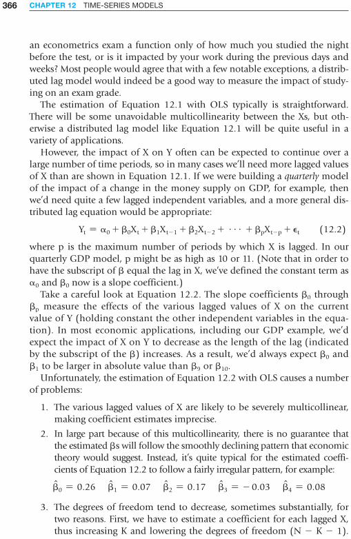
366 ChapTEr 12 tiMe-series MoDeLs
an econometrics exam a function only of how much you studied the night before the test, or is it impacted by your work during the previous days and weeks? Most people would agree that with a few notable exceptions, a distrib-uted lag model would indeed be a good way to measure the impact of study-ing on an exam grade.
The estimation of Equation 12.1 with OLS typically is straightforward. There will be some unavoidable multicollinearity between the Xs, but oth-erwise a distributed lag model like Equation 12.1 will be quite useful in a variety of applications.
However, the impact of X on Y often can be expected to continue over a large number of time periods, so in many cases we’ll need more lagged values of X than are shown in Equation 12.1. If we were building a quarterly model of the impact of a change in the money supply on GDP, for example, then we’d need quite a few lagged independent variables, and a more general dis-tributed lag equation would be appropriate:
Yt = α0 + β0Xt + β1Xt - 1 + β2Xt - 2 + g + βpXt - p + et (12.2)
where p is the maximum number of periods by which X is lagged. In our quarterly GDP model, p might be as high as 10 or 11. (Note that in order to have the subscript of β equal the lag in X, we’ve defined the constant term as α0 and β0 now is a slope coefficient.)
Take a careful look at Equation 12.2. The slope coefficients β0 through βp measure the effects of the various lagged values of X on the current value of Y (holding constant the other independent variables in the equa-tion). In most economic applications, including our GDP example, we’d expect the impact of X on Y to decrease as the length of the lag (indicated by the subscript of the β) increases. As a result, we’d always expect β0 and β1 to be larger in absolute value than β9 or β10.
Unfortunately, the estimation of Equation 12.2 with OLS causes a number of problems:
1. The various lagged values of X are likely to be severely multicollinear, making coefficient estimates imprecise.
2. In large part because of this multicollinearity, there is no guarantee that the estimated βs will follow the smoothly declining pattern that economic theory would suggest. Instead, it’s quite typical for the estimated coeffi-cients of Equation 12.2 to follow a fairly irregular pattern, for example:
βn0 = 0.26 βn1 = 0.07 βn2 = 0.17 βn3 = - 0.03 βn4 = 0.08
3. The degrees of freedom tend to decrease, sometimes substantially, for two reasons. First, we have to estimate a coefficient for each lagged X, thus increasing K and lowering the degrees of freedom (N 2 K 2 1).
M12_STUD2742_07_SE_C12.indd 366 1/9/16 2:19 PM

367 DynaMic MoDeLs
Second, unless data for lagged Xs outside the sample are available, we have to decrease the sample size by 1 for each lagged X we calculate, thus lowering the number of observations, N, and therefore the degrees of freedom.
As a result of these problems with OLS estimation of distributed lag equa-tions like Equation 12.2, it’s standard practice to consider a simplifying assumption in such situations. The most commonly used simplification is to replace all the lagged independent variables with a lagged value of the depen-dent variable, and we’ll call that kind of equation a dynamic model.
12.2 Dynamic Models
The simplest dynamic model is:
Yt = α0 + β0Xt + λYt - 1 + ut (12.3)
Note that Y is on both sides of the equation! Luckily, the subscripts are differ-ent in that the Y on the left-hand side is Yt, and the Y on the right-hand side is Yt−1. It’s this difference in time period that makes the equation dynamic. Thus, the simplest dynamic model is an equation in which the current value of the dependent variable Y is a function of the current value of X and a lagged value of Y itself. Such a model with a lagged dependent variable is often called an autoregressive equation.
Let’s look at Equation 12.3 to try to see why it can be used to represent a distributed lag model or any model in which the impact of X on Y is dis-tributed over a number of lags. Suppose that we lag Equation 12.3 one time period:
Yt - 1 = α0 + β0Xt - 1 + λYt - 2 + ut - 1 (12.4)
If we now substitute Equation 12.4 for Yt - 1 in Equation 12.3, we get:
Yt = α0 + β0Xt + λ1α0 + β0Xt - 1 + λYt - 2 + ut - 12 + ut (12.5)
or
Yt = 1α0 + λα02 + β0Xt + λβ0Xt - 1 + λ2Yt - 2 + 1λut - 1 + ut2 (12.6)
If we do this one more time (that is, if we lag Equation 12.3 two time peri-ods, substitute it into Equation 12.5, and rearrange), we get:
Yt = α0* + β0Xt + λβ0Xt - 1 + λ2β0Xt - 2 + λ3Yt - 3 + ut* (12.7)
M12_STUD2742_07_SE_C12.indd 367 1/9/16 2:19 PM
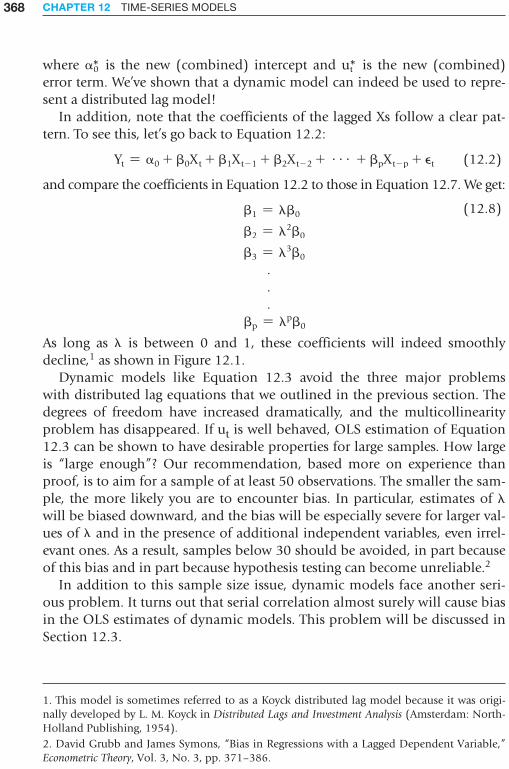
368 ChapTEr 12 tiMe-series MoDeLs
where α0* is the new (combined) intercept and ut* is the new (combined) error term. We’ve shown that a dynamic model can indeed be used to repre-sent a distributed lag model!
In addition, note that the coefficients of the lagged Xs follow a clear pat-tern. To see this, let’s go back to Equation 12.2:
Yt = α0 + β0Xt + β1Xt - 1 + β2Xt - 2 + g + βpXt - p + et (12.2)
and compare the coefficients in Equation 12.2 to those in Equation 12.7. We get:
β1 = λβ0
β2 = λ2β0
β3 = λ3β0
. . . βp = λpβ0
(12.8)
As long as λ is between 0 and 1, these coefficients will indeed smoothly decline,1 as shown in Figure 12.1.
Dynamic models like Equation 12.3 avoid the three major problems with distributed lag equations that we outlined in the previous section. The degrees of freedom have increased dramatically, and the multicollinearity problem has disappeared. If ut is well behaved, OLS estimation of Equation 12.3 can be shown to have desirable properties for large samples. How large is “large enough”? Our recommendation, based more on experience than proof, is to aim for a sample of at least 50 observations. The smaller the sam-ple, the more likely you are to encounter bias. In particular, estimates of λ will be biased downward, and the bias will be especially severe for larger val-ues of λ and in the presence of additional independent variables, even irrel-evant ones. As a result, samples below 30 should be avoided, in part because of this bias and in part because hypothesis testing can become unreliable.2
In addition to this sample size issue, dynamic models face another seri-ous problem. It turns out that serial correlation almost surely will cause bias in the OLS estimates of dynamic models. This problem will be discussed in Section 12.3.
1. This model is sometimes referred to as a Koyck distributed lag model because it was origi-nally developed by L. M. Koyck in Distributed Lags and Investment Analysis (Amsterdam: North-Holland Publishing, 1954).2. David Grubb and James Symons, “Bias in Regressions with a Lagged Dependent Variable,” Econometric Theory, Vol. 3, No. 3, pp. 371–386.
M12_STUD2742_07_SE_C12.indd 368 1/9/16 2:19 PM

369 Dynamic moDels
An Example of a Dynamic Model
As an example of a dynamic model, let’s look at an aggregate consumption function from a macroeconomic equilibrium GDP model. Many econo-mists argue that in such a model, consumption (COt) is not just an instan-taneous function of disposable income (YDt). Instead, they believe that current consumption is also influenced by past levels of disposable income (YDt - 1, YDt - 2, etc.):
COt = α0 + β0YDt + β1YDt - 1 + β2YDt - 2 + g + βpYDt - p + et (12.9)
Such an equation fits well with simple models of consumption, but it makes sense only if the coefficients of past levels of income decrease as the length of the lag increases. That is, the impact of lagged income on current consump-tion should decrease as the lag gets bigger. Thus we’d expect the coefficient of YDt - 2 to be less than the coefficient of YDt - 1, and so on.
As a result, most econometricians would model Equation 12.9 with a dynamic model:
COt = α0 + β0YDt + λCOt - 1 + ut (12.10)
0 1 2 3 4
l 5 0.75
l 5 0.50
l 5 0.02
5 6 7
1.0
0.5
Rel
ativ
e W
eigh
t of
Lag
ged
Var
iabl
e
Time Period of Lag
Figure 12.1 Geometric Weighting schemes for Various Dynamic models
As long as λ is between 0 and 1, a dynamic model has the impact of the independent variable declining as the length of the lag increases.
M12_STUD2742_07_SE_C12.indd 369 21/01/16 1:50 PM
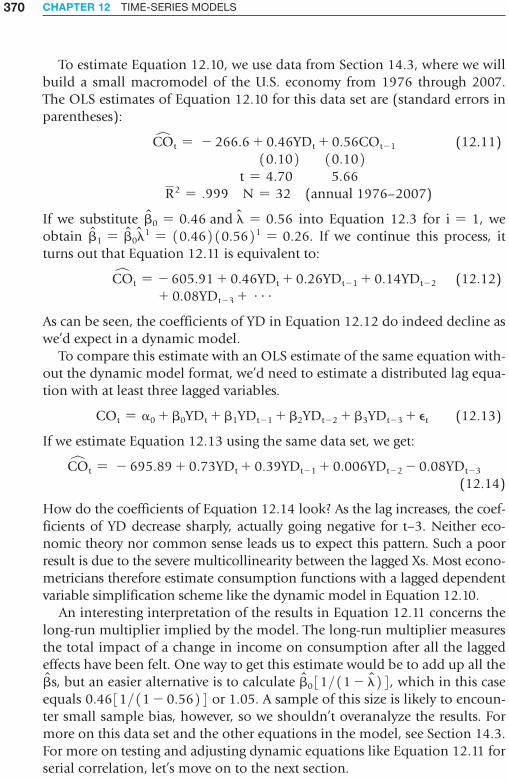
370 ChapTEr 12 tiMe-series MoDeLs
To estimate Equation 12.10, we use data from Section 14.3, where we will build a small macromodel of the U.S. economy from 1976 through 2007. The OLS estimates of Equation 12.10 for this data set are (standard errors in parentheses):
COt = - 266.6 + 0.46YDt + 0.56COt - 1 (12.11) 10.102 10.102 t = 4.70 5.66 R
2 = .999 N = 32 (annual 1976–2007)
If we substitute βn0 = 0.46 and λn = 0.56 into Equation 12.3 for i = 1, we obtain βn1 = βn 0λn 1 = 10.46210.5621 = 0.26. If we continue this process, it turns out that Equation 12.11 is equivalent to:
COt = - 605.91 + 0.46YDt + 0.26YDt - 1 + 0.14YDt - 2
+ 0.08YDt - 3 + g (12.12)
As can be seen, the coefficients of YD in Equation 12.12 do indeed decline as we’d expect in a dynamic model.
To compare this estimate with an OLS estimate of the same equation with-out the dynamic model format, we’d need to estimate a distributed lag equa-tion with at least three lagged variables.
COt = α0 + β0YDt + β1YDt - 1 + β2YDt - 2 + β3YDt - 3 + et (12.13)
If we estimate Equation 12.13 using the same data set, we get:
COt = - 695.89 + 0.73YDt + 0.39YDt - 1 + 0.006YDt - 2 - 0.08YDt - 3
(12.14)
How do the coefficients of Equation 12.14 look? As the lag increases, the coef-ficients of YD decrease sharply, actually going negative for t−3. Neither eco-nomic theory nor common sense leads us to expect this pattern. Such a poor result is due to the severe multicollinearity between the lagged Xs. Most econo-metricians therefore estimate consumption functions with a lagged dependent variable simplification scheme like the dynamic model in Equation 12.10.
An interesting interpretation of the results in Equation 12.11 concerns the long-run multiplier implied by the model. The long-run multiplier measures the total impact of a change in income on consumption after all the lagged effects have been felt. One way to get this estimate would be to add up all the βns, but an easier alternative is to calculate βn031> 11 - λn24, which in this case equals 0.4631> 11 - 0.5624 or 1.05. A sample of this size is likely to encoun-ter small sample bias, however, so we shouldn’t overanalyze the results. For more on this data set and the other equations in the model, see Section 14.3. For more on testing and adjusting dynamic equations like Equation 12.11 for serial correlation, let’s move on to the next section.
9
9
9
M12_STUD2742_07_SE_C12.indd 370 1/9/16 2:19 PM

371 seriaL correLation anD DynaMic MoDeLs
12.3 Serial Correlation and Dynamic Models
The consequences of serial correlation depend crucially on the type of model we’re talking about. For a distributed lag model such as Equation 12.2, serial correlation has the effects outlined in Section 9.3: Serial correlation causes: (1) OLS to no longer be the minimum variance unbiased estimator, (2) the SE(βn)s to be biased, and (3) no bias in the OLS βns themselves.
For dynamic models such as Equation 12.3, however, all this changes, and serial correlation does indeed cause bias in the βns produced by OLS. Com-pounding this is the fact that the detection of and remedies for serial correla-tion that we discussed in Chapter 9 need to be modified in the presence of a lagged dependent variable.
Serial Correlation Causes Bias in Dynamic Models
If an equation with a lagged dependent variable as an independent variable has a serially correlated error term, then OLS estimates of the coefficients will be biased, even in large samples.
To see where this bias comes from, let’s start with a dynamic model:
Yt = α0 + β0Xt + λYt - 1 + ut (12.3)
and lag it one time period:
c c Yt - 1 = α0 + β0Xt - 1 + λYt - 2 + ut - 1 (12.15)
As you can see from the upward-pointing arrows above Equation 12.15, if ut - 1 is positive, then Yt - 1 will be higher than it would have been otherwise.
In addition, if ut is serially correlated, then we know that:
c c ut = ρut - 1 + et (12.16)
where et is a classical error term with an expected value of zero. As you can see from the arrows above Equation 12.16, if ut - 1 is positive, then ut will be higher than it would have been otherwise as long as ρ is positive, as it typi-cally is in economic applications.
If we add the arrows from Equations 12.15 and 12.16 to Equation 12.3, we get:
c c Yt = α0 + β0Xt + λYt - 1 + ut (12.3)
Take a look at the arrows in Equation 12.3. Yt - 1 and ut are correlated! Such a correlation violates Classical Assumption III, which assumes that the error
M12_STUD2742_07_SE_C12.indd 371 1/9/16 2:19 PM

372 ChapTEr 12 tiMe-series MoDeLs
term is not correlated with any of the explanatory variables. (If ut - 1 is nega-tive, then both ut and Yt - 1 will be lower than they would have been other-wise, which again violates Classical Assumption III.)
The consequences of this correlation include biased estimates, in particu-lar of the coefficient λ, because OLS attributes to Yt - 1 some of the change in Yt actually caused by ut. In essence, the uncorrected serial correlation acts like an omitted variable (ut - 1). Since an omitted variable causes bias whenever it is correlated with one of the included independent variables, and since ut - 1 is correlated with Yt - 1, the combination of a lagged dependent variable and serial correlation causes bias in the coefficient estimates. This bias is in addi-tion to the bias mentioned on page 368.
Testing for Serial Correlation in Dynamic Models
If serial correlation causes bias in a dynamic model, then tests for serial corre-lation are obviously important. Unfortunately, however, the Durbin–Watson test is potentially invalid for an equation that contains a lagged dependent variable as an independent variable because the Durbin–Watson statistic is biased toward 2 in a dynamic equation. This bias toward 2 means that serial correlation in a dynamic model is more likely to evade detection by the Durbin–Watson test.3
Luckily, the Lagrange Multiplier (LM) serial correlation test of Section 9.4 still is valid even in the face of a lagged dependent variable. Using the Lagrange Multiplier to test for serial correlation in a typical dynamic model involves three steps that should seem familiar:
1. Obtain the residuals from the estimated equation:
et = Yt - Ynt = Yt - αn 0 - βn 0X1t - λn Yt - 1 (12.17)
2. Use these residuals as the dependent variable in an auxiliary equation that includes as independent variables all those on the right-hand side of the original equation as well as the lagged residuals:
et = a0 + a1Xt + a2Yt - 1 + a3et - 1 + ut (12.18)
3. The opposite is not a problem. A Durbin−Watson test that indicates serial correlation in the presence of a lagged dependent variable, despite the bias toward 2, is an even stronger affirma-tion of serial correlation.
M12_STUD2742_07_SE_C12.indd 372 1/9/16 2:19 PM

373 seriaL correLation anD DynaMic MoDeLs
3. Estimate Equation 12.18 using OLS and then test the null hypothesis that a3 = 0 with the following test statistic:
LM = NR2 (12.19)
where N is the sample size and R2 is the unadjusted coefficient of de-termination, both of the auxiliary equation, Equation 12.18. For large samples, NR2 has a chi-square distribution with degrees of freedom equal to the number of restrictions in the null hypothesis (in this case, one). If NR2 is greater than the critical chi-square value from Statistical Table B-6, then we reject the null hypothesis that a3 = 0 and conclude that there is indeed serial correlation in the original equation.
As an example of testing for serial correlation in a dynamic model, let’s run a Lagrange Multiplier (LM) serial correlation test on Equation 12.11, the consumption function we estimated in the previous section. If we estimate the auxiliary equation for that model, we get an R2 of .4025 which, when multiplied by the sample size of 31 (do you see why it’s 31 and not 32?), produces an NR2 of 12.48. 12.48 is greater than 3.84, the 5-percent critical chi-square value with one degree of freedom, so we have strong evidence of serial correlation in Equation 12.11. What should we do?
Correcting for Serial Correlation in Dynamic Models
If the Lagrange Multiplier test indicates serial correlation in a dynamic model, the first step is to consider the possibility that the serial correlation is impure, perhaps caused by omission of a relevant variable and/or by failure to capture the actual distributed lag pattern accurately.
If the serial correlation appears to be pure, then the theoretically preferred solution is to transform the equation so as to eliminate the serial correlation and re-estimate the model. The required transformation is quite similar to the Generalized Least Squares approach to serial correlation described in Sec-tion 9.5. Unfortunately, the iterative nonlinear estimation of the transformed equation is well beyond the scope of this text, so it’s not a realistic alternative for most readers.4 Instead, our suggestion is to use one of two alternatives, depending on the underlying theory of the model and the size of the sample.
If theory indicates that only a few lagged values of X are meaningful in explaining Y, then a potential way to avoid the bias due to serial correlation
4. Readers interested in this approach should see Sean Becketti, “Introduction to Time Series Using Stata” (College Station: Stata Press, 2013), pp. 192–195.
M12_STUD2742_07_SE_C12.indd 373 1/9/16 2:19 PM

374 ChapTEr 12 tiMe-series MoDeLs
is to estimate a distributed lag model (Equation 12.2 with p = 1 or 2) instead of a dynamic model. The distributed lag model will have potential multicollinearity but will not likely face the other problems typically associ-ated with distributed lag models because p is so low. Most econometricians would prefer to deal with the consequences of multicollinearity than to face bias, so this is an improvement. There’s a second advantage to distributed lags. The Xt - p terms, in essence, are acting as proxies for Yt - 1. As we’ll learn in Chapter 14, such proxies are similar to instrumental variables, and they are especially useful because they will eliminate bias if they’re uncorrelated with the error term.
In a small sample, the best approach may well be to continue to use OLS even in the face of serial correlation in a dynamic model. For a nontrivial subset of real-world examples, OLS actually outperforms more sophisticated techniques. One reason is that in a small sample, the estimation bias in λ men-tioned in Section 12.2 and the bias introduced by serial correlation often are of opposite signs, so they offset each other. As a result, OLS can do better than a technique that eliminates only the bias caused by serial correlation.5 The second reason is that there’s evidence from Monte Carlo studies that the size of the bias introduced by serial correlation in small samples often is fairly low.6
To sum, unless you’re comfortable with iterative nonlinear least squares, our suggestion for dealing with serial correlation in dynamic models depends on theory and the sample size. If theory calls for very few lagged Xs, we sug-gest the distributed lag approach. If the sample is small, we think continuing to use OLS, even in the face of serial correlation, presents the best alternative. If both the sample and the meaningful number of lagged Xs are large, we’d recommend using distributed lags because of the benefits of the instrumental variable approach.
12.4 Granger Causality
One application of distributed lag models is to provide evidence about the direction of causality in economic relationships. Such a test is useful when we know that two variables are related but we don’t know which variable causes the other to move. For example, most economists believe that increases in the
5. Asatoshi Maeshiro, “Teaching Regressions with a Lagged Dependent Variable and Autocor-related Disturbances,” Journal of Economic Education, Vol. 27, No. 1, pp. 72–84.
6. Luke Keele and Nathan Kelly, “Dynamic Models for Dynamic Theories: The Ins and Outs of Lagged Dependent Variables,” Political Analysis, Vol. 14, No. 2, pp. 186–205.
M12_STUD2742_07_SE_C12.indd 374 1/9/16 2:19 PM
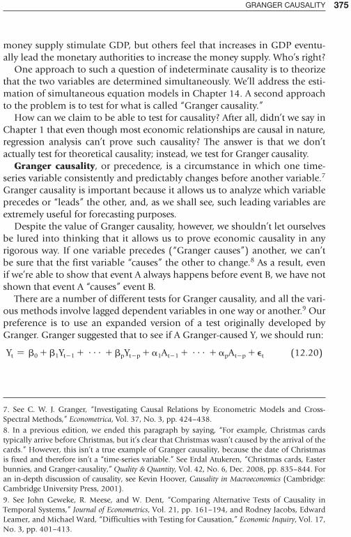
375 granger causaLity
money supply stimulate GDP, but others feel that increases in GDP eventu-ally lead the monetary authorities to increase the money supply. Who’s right?
One approach to such a question of indeterminate causality is to theorize that the two variables are determined simultaneously. We’ll address the esti-mation of simultaneous equation models in Chapter 14. A second approach to the problem is to test for what is called “Granger causality.”
How can we claim to be able to test for causality? After all, didn’t we say in Chapter 1 that even though most economic relationships are causal in nature, regression analysis can’t prove such causality? The answer is that we don’t actually test for theoretical causality; instead, we test for Granger causality.
Granger causality, or precedence, is a circumstance in which one time-series variable consistently and predictably changes before another variable.7 Granger causality is important because it allows us to analyze which variable precedes or “leads” the other, and, as we shall see, such leading variables are extremely useful for forecasting purposes.
Despite the value of Granger causality, however, we shouldn’t let ourselves be lured into thinking that it allows us to prove economic causality in any rigorous way. If one variable precedes (“Granger causes”) another, we can’t be sure that the first variable “causes” the other to change.8 As a result, even if we’re able to show that event A always happens before event B, we have not shown that event A “causes” event B.
There are a number of different tests for Granger causality, and all the vari-ous methods involve lagged dependent variables in one way or another.9 Our preference is to use an expanded version of a test originally developed by Granger. Granger suggested that to see if A Granger-caused Y, we should run:
Yt = β0 + β1Yt - 1 + g + βpYt - p + α1At - 1 + g + αpAt - p + et (12.20)
7. See C. W. J. Granger, “Investigating Causal Relations by Econometric Models and Cross-Spectral Methods,” Econometrica, Vol. 37, No. 3, pp. 424−438.8. In a previous edition, we ended this paragraph by saying, “For example, Christmas cards typically arrive before Christmas, but it’s clear that Christmas wasn’t caused by the arrival of the cards.” However, this isn’t a true example of Granger causality, because the date of Christmas is fixed and therefore isn’t a “time-series variable.” See Erdal Atukeren, “Christmas cards, Easter bunnies, and Granger-causality,” Quality & Quantity, Vol. 42, No. 6, Dec. 2008, pp. 835–844. For an in-depth discussion of causality, see Kevin Hoover, Causality in Macroeconomics (Cambridge: Cambridge University Press, 2001).9. See John Geweke, R. Meese, and W. Dent, “Comparing Alternative Tests of Causality in Temporal Systems,” Journal of Econometrics, Vol. 21, pp. 161−194, and Rodney Jacobs, Edward Leamer, and Michael Ward, “Difficulties with Testing for Causation,” Economic Inquiry, Vol. 17, No. 3, pp. 401−413.
M12_STUD2742_07_SE_C12.indd 375 1/9/16 2:19 PM
376 ChapTEr 12 tiMe-series MoDeLs
and test the null hypothesis that the coefficients of the lagged As (the αs) jointly equal zero.10 If we can reject this null hypothesis using the F-test, then we have evidence that A Granger-causes Y. Note that if p = 0, Equation 12.20 is similar to the dynamic model, Equation 12.3.
Applications of this test involve running two Granger tests, one in each direction. That is, run Equation 12.20 and also run:
At = β0 + β1At - 1 + g + βpAt - p + α1Yt - 1 + g + αpYt - p + et (12.21)
testing for Granger causality in both directions by testing the null hypothesis that the coefficients of the lagged Ys (again, the αs) jointly equal zero. If the F-test is significant for Equation 12.20 but not for Equation 12.21, then we can conclude that A Granger-causes Y.
12.5 Spurious Correlation and Nonstationarity
One problem with time-series data is that independent variables can appear to be more significant than they actually are if they have the same underly-ing trend as the dependent variable. In a country with rampant inflation, for example, almost any nominal variable will appear to be highly correlated with all other nominal variables. Why? Nominal variables are unadjusted for inflation, so every nominal variable will have a powerful inflationary component. This inflationary component will usually outweigh any real causal relationship, making nominal variables appear to be correlated even if they aren’t.
Such a problem is an example of spurious correlation, a strong relation-ship between two or more variables that is not caused by a real underlying causal relationship. If you run a regression in which the dependent variable and one or more independent variables are spuriously correlated, the result is a spurious regression, and the t-scores and overall fit of such spurious regres-sions are likely to be overstated and untrustworthy.
There are many causes of spurious correlation. In a cross-sectional data set, for example, spurious correlation can be caused by dividing both the dependent variable and at least one independent variable by a third variable that varies considerably more than do the others. The focus of this section, however, will be on time-series data and in particular on spurious correlation caused by nonstationary time series.
10. Such a joint test requires the use of the F-test of Section 5.6.
M12_STUD2742_07_SE_C12.indd 376 1/9/16 2:19 PM

377 spurious correLation anD nonstationarity
Stationary and Nonstationary Time Series
A stationary series is one whose basic properties, for example, its mean and its variance, do not change over time. In contrast, a nonstationary series has one or more basic properties that do change over time. For instance, the real per capita output of an economy typically increases over time, so it’s nonsta-tionary. By contrast, the growth rate of real per capita output often does not increase over time, so this variable is stationary even though the variable it’s based on, real per capita output, is nonstationary. A time series can be non-stationary even with a constant mean if another property, such as the vari-ance, changes over time.
More formally, a time-series variable, Xt, is stationary if:
1. the mean of Xt is constant over time,
2. the variance of Xt is constant over time, and
3. the simple correlation coefficient between Xt and Xt - k depends on the length of the lag (k) but on no other variable (for all k).11
If one or more of these properties is not met, then Xt is nonstationary. And if a series is nonstationary, that problem is referred to as nonstationarity.
Although our definition of a stationary series focuses on stationary and nonstationary variables, it’s important to note that error terms (and, therefore, residuals) also can be nonstationary. In fact, we’ve already had experience with a nonstationary error term. Many cases of heteroskedasticity in time-series data involve an error term with a variance that tends to increase with time. That kind of heteroskedastic error term is also nonstationary!
The major consequence of nonstationarity for regression analysis is spuri-ous correlation that inflates R2 and the t-scores of the nonstationary inde-pendent variables, which in turn leads to incorrect model specification. This occurs because the regression estimation procedure attributes to the nonsta-tionary Xt changes in Yt that were actually caused by some factor (trend, for example) that also affects Xt. Thus, the variables move together because of the nonstationarity, increasing R2 and the relevant t-scores. This is especially
11. There are two different definitions of stationarity. The particular definition we use here is a simplification of the most frequently cited definition, referred to by various authors as weak, wide-sense, or covariance stationarity. In addition, there are many models of nonstationarity, for example ARCH and GARCH, that are significantly more sophisticated than the model of nonstationarity introduced in this section.
M12_STUD2742_07_SE_C12.indd 377 1/9/16 2:19 PM

378 ChAptEr 12 Time-series moDels
important in macroeconometrics, and the macroeconomic literature includes many articles that examine various series for signs of nonstationarity.12
Some variables are nonstationary mainly because they increase rapidly over time. Spurious regression results involving these kinds of variables often can be avoided by the addition of a simple time trend 1t = 1, 2, 3, c , T2 to the equation as an independent variable.
Unfortunately, many economic time-series variables are nonstationary even after the removal of a time trend. This nonstationarity often takes the form of the variable behaving as though it were a “random walk.” A random walk is a time-series variable in which the next period’s value equals this period’s value plus a stochastic error term. A random-walk variable is nonsta-tionary because it can wander up and down without an inherent equilibrium and without approaching a long-term mean of any sort.
To get a better understanding of how a random walk gives rise to nonsta-tionarity, let’s suppose that Yt is generated by an equation that includes only past values of itself (an autoregressive equation):
Yt = γYt - 1 + vt (12.22)
where vt is a classical error term.Take a look at Equation 12.22. Can you see that if 0 γ 0 6 1, then the
expected value of Yt will eventually approach 0 (and therefore be stationary) as the sample size gets bigger and bigger? (Remember, since vt is a classical error term, its expected value = 0.) Similarly, can you see that if 0 γ 0 7 1, then the expected absolute value of Yt will continuously increase, making Yt nonstationary? This is nonstationarity due to a trend, but it still can cause spurious regression results.
Most importantly, what about if 0 γ 0 = 1? In this case,
Yt = Yt - 1 + vt (12.23)
It’s a random walk! The expected value of Yt does not converge on any value, meaning that it is nonstationary. This circumstance, where γ = 1 in Equation 12.23 (or similar equations), is called a unit root. If a variable has a unit root, then Equation 12.23 holds, and the variable follows a random walk and is nonstationary. The relationship between unit roots and nonstationarity is so strong that some econometricians use the words interchangeably, even though they recognize that many factors other than unit roots can cause nonstationarity.
12. See, for example, C. R. Nelson and C. I. Plosser, “Trends and Random Walks in Macroeco-nomics Time Series: Some Evidence and Implication,” Journal of Monetary Economics, Vol. 10, pp. 169−182, and J. Campbell and N. G. Mankiw, “Permanent and Transitory Components in Macroeconomic Fluctuations,” American Economic Review, Vol. 77, No. 2, pp. 111−117.
M12_STUD2742_07_SE_C12.indd 378 21/01/16 1:50 PM

379 spurious correLation anD nonstationarity
Spurious regression
As noted at the beginning of this section, if the dependent variable and at least one independent variable in an equation are trending, as they will if they contain unit roots, it’s possible for the results of an OLS regression to be spurious.13
Consider the linear regression model
Yt = α0 + β0Xt + ut (12.24)
If both X and Y are nonstationary, then they can be highly correlated for non-causal reasons, and our standard regression inference measures will be very misleading in that they’ll overstate R
2 and the t-score for βn0.For example, take a look at the following estimated equation:
PRICEt = -27.8 + 0.070TUITIONt
10.0062 t = 11.4 R
2 = .94 T = 101annual2
(12.25)
The R
2 of this equation and the t-score for the coefficient of TUITION are clearly significant, but what are the definitions of the variables? Well, PRICE is the price of a gallon of gasoline in Portland, Oregon, and TUITION is the tuition for a semester of study at Occidental College (Oxy) in Los Angeles (both measured in nominal dollars). Is it possible that an increase in the tuition at Oxy caused gas prices in Portland to go up? Not unless every Oxy student was the child of a Portland gas station owner! What’s going on? Well, this regression is from the 1970s, a decade of inflation, so any nominally measured variables are likely to result in an equation that fits as well as Equation 12.25. Both vari-ables are nonstationary, and this particular regression result clearly is spurious.
To avoid spurious regression results, it’s crucial to be sure that time-series variables are stationary before running regressions.
The Dickey–Fuller Test
To ensure that the equations we estimate are not spurious, it’s important to test for nonstationarity. If we can be reasonably sure that all the variables are stationary, then we need not worry about spurious regressions. How can you tell if a time series is nonstationary? The first step is to visually examine the
h
13. See C. W. J. Granger and P. Newbold, “Spurious Regression in Econometrics,” Journal of Econometrics, Volume 2, pp. 111–120.
M12_STUD2742_07_SE_C12.indd 379 1/9/16 2:19 PM

380 ChapTEr 12 tiMe-series MoDeLs
data. For many time series, a quick glance at the data (or a diagram of the data) will tell you that the mean of a variable is increasing dramatically over time and that the series is nonstationary.
After this trend has been removed, the standard method of testing for non-stationarity is the Dickey–Fuller test,14 which examines the hypothesis that the variable in question has a unit root15 and, as a result, is likely to benefit from being expressed in first-difference form.
To best understand how the Dickey–Fuller test works, let’s return to the discussion of the role that unit roots play in the distinction between station-arity and nonstationarity. Recall that we looked at the value of γ in Equation 12.22 to help us determine if Y was stationary or nonstationary:
Yt = γYt - 1 + vt (12.22)
We decided that if 0 γ 0 6 1, then Y is stationary, and that if 0 γ 0 7 1, then Yt is nonstationary. However, if 0 γ 0 = 1, then Yt is nonstationary due to a unit root. Thus we concluded that the autoregressive model is stationary if 0 γ 0 6 1 and nonstationary otherwise.
From this discussion of stationarity and unit roots, it makes sense to esti-mate Equation 12.22 and determine if 0 γ 0 6 1 to see if Y is stationary, and that’s almost exactly how the Dickey–Fuller test works. First, we subtract Yt−1 from both sides of Equation 12.22, yielding:
1Yt - Yt - 12 = 1γ - 12Yt - 1 + vt (12.26)
If we define ∆Yt = Yt - Yt - 1 then we have the simplest form of the Dickey–Fuller test:
∆Yt = β1Yt - 1 + vt (12.27)
where β1 = γ - 1. The null hypothesis is that Yt contains a unit root and is therefore nonstationary, and the alternative hypothesis is that Yt is stationary. If Yt contains a unit root, γ = 1 and β1 = 0. If Yt is stationary, 0 γ 0 6 1 and β1 6 0. Hence we construct a one-sided t-test on the hypothesis that β1 = 0:
H0: β1 = 0 HA: β1 6 0
14. D. A. Dickey and W. A. Fuller, “Distribution of the Estimators for Autoregressive Time-Series with a Unit Root,” Journal of the American Statistical Association, Vol. 74, pp. 427–431.15. For more on unit roots, see John Y. Campbell and Pierre Peron, “Pitfalls and Opportuni-ties: What Macroeconomists Should Know About Unit Roots,” NBER Macroeconomics Annual (Cambridge, MA: MIT Press, 1991), pp. 141–219.
M12_STUD2742_07_SE_C12.indd 380 1/9/16 2:19 PM

381 spurious correLation anD nonstationarity
The Dickey–Fuller test actually comes in three versions:
1. Equation 12.27,
2. Equation 12.27 with a constant term added (Equation 12.28), and
3. Equation 12.27 with a constant term and a trend term added (Equation 12.29).
The form of the Dickey–Fuller test in Equation 12.27 is correct if Yt follows Equation 12.22, but most econometricians add a constant term to the equa-tion, for reasons similar to those mentioned in Section 7.1, so the basic Dickey–Fuller test equation becomes:
∆Yt = β0 + β1Yt - 1 + vt (12.28)
Alternatively, if we believe Yt contains a trend “t” 1t = 1, 2, 3, c , T2, then we’d add “t” to the equation as a variable with a coefficient, and the appropri-ate Dickey–Fuller test equation is:
∆Yt = β0 + β1Yt - 1 + β2t + vt (12.29)
How do we decide whether to use Equation 12.28 or Equation 12.29? If you compare the two equations, you can see that the only difference between them is a trend term (β2t) that’s in Equation 12.29 but not in Equation 12.28. Thus Equation 12.29 is appropriate if Y is growing and Equation 12.28 is appropriate if Y is not growing. Perhaps the best way to make this decision is to plot Y over time and then judge whether or not it appears to be growing.16 GDP and consumption are good examples of variables that usually are grow-ing over time, while most rates (like interest rates and unemployment rates) are good examples of variables that are not growing.
No matter which form of the Dickey–Fuller test we use, the decision rule is the same. If βn1 is significantly less than 0 as measured by a t-test, then we can reject the null hypothesis of a unit root; this implies that the variable is stationary. If βn1 is not significantly less than 0, then we cannot reject the null hypothesis of a unit root; this implies that the variable is nonstationary. (Recall from Chapter 5 that if we’re not able to reject the null hypothesis, we still have not “proven” that Y is nonstationary.)
16. John Elder and Peter Kennedy, “Testing for Unit Roots: What Should Students Be Taught?” Journal of Economic Education, Vol. 32, No. 2, pp. 137–146. Elder and Kennedy also investigate what to do in the unlikely case that the growth status of Y is unknown.
M12_STUD2742_07_SE_C12.indd 381 1/9/16 2:19 PM

382 ChapTEr 12 tiMe-series MoDeLs
Be careful, however. The standard t-table does not apply to Dickey–Fuller tests. Instead the critical values are somewhat higher than those in Statistical Table B-1, and they also depend on the version of the Dickey–Fuller test you use. In Table 12.1,17 we list critical values for the two versions of the Dickey–Fuller test we have discussed the most, Equations 12.28 and 12.29. For exam-ple, a 5-percent one-sided test of β1 in Equation 12.28 with a sample size of 25 has a critical t-value of 3.00 compared to 1.717 for a standard t-test (with 22 degrees of freedom since K = 2).
The Dickey–Fuller specifications in Equations 12.28 and 12.29 and the critical values for those specifications are derived under the assumption that the error term is serially uncorrelated. If the error term is serially correlated, then the test must be modified to take this serial correlation into account. This adjustment, called the Augmented Dickey–Fuller test (ADF), adds a series of lagged values of ∆Y to the Dickey–Fuller test. While the ADF is the most-used version of the Dickey–Fuller test, it is beyond the scope of this textbook, at least in part because choosing how many lagged ∆Y values to include can be quite complicated.
Cointegration
If the Dickey–Fuller test reveals nonstationarity, what should we do?The traditional approach is to take the first differences (∆Y = Yt - Yt - 1
and ∆X = Xt - Xt - 1) and use them in place of Yt and Xt in the equation.
17. Most sources list negative critical values for the Dickey–Fuller test, because the unit root test is one-sided with a negative expected value. However, the t-test decision rule of this text is based on the absolute value of the t-score, so negative critical values would cause every null hypoth-esis to be rejected. As a result, the critical values in Table 12.1 are positive. For adjusted critical t-values for the Dickey–Fuller test, including those in Table 12.1, see J. G. MacKinnon, “Criti-cal Values of Cointegration Tests,” in Rob Engle and C. W. J. Granger, eds., Long-Run Economic Relationships: Readings in Cointegration (New York: Oxford University Press, 1991), Chapter 13. Most software packages provide these critical values with the output from a Dickey–Fuller test.
Table 12.1 5-percent one-sided critical Values for the Dickey–Fuller test
Sample Size (T)
For Equation 12.28 (Y not growing)
For Equation 12.29 (Y growing)
25 3.00 3.60
50 2.93 3.50
100 2.89 3.45
∞ 2.86 3.41
M12_STUD2742_07_SE_C12.indd 382 1/9/16 2:19 PM

383 spurious correLation anD nonstationarity
With economic data, taking a first difference usually is enough to convert a nonstationary series into a stationary one. Unfortunately, using first differ-ences to correct for nonstationarity throws away information that economic theory can provide in the form of equilibrium relationships between the vari-ables when they are expressed in their original units (Xt and Yt). As a result, first differences should not be used without carefully weighing the costs and benefits of that shift, and in particular first differences should not be used until the residuals have been tested for cointegration.
Cointegration consists of matching the degree of nonstationarity of the variables in an equation in a way that makes the error term (and residuals) of the equation stationary and rids the equation of any spurious regression results. Even though individual variables might be nonstationary, it’s possible for linear combinations of nonstationary variables to be stationary, or cointe-grated. If a long-run equilbrium relationship exists between a set of variables, those variables are said to be cointegrated. If the variables are cointegrated, then you can avoid spurious regressions even though the dependent variable and at least one independent variable are nonstationary.
To see how this works, let’s return to Equation 12.24:
Yt = α0 + β0Xt + ut (12.24)
As we saw in the previous section, if Xt and Yt are nonstationary, it’s likely that we’ll get spurious regression results. To understand how it’s possible to get sensible results from Equation 12.24 if the nonstationary variables are cointegrated, let’s focus on the case in which both Xt and Yt contain one unit root. The key to cointegration is the behavior of ut.
If we solve Equation 12.24 for ut, we get:
ut = Yt - α0 - β0Xt (12.30)
In Equation 12.30, ut is a function of two nonstationary variables, so you’d certainly expect ut also to be nonstationary, but that’s not necessarily the case. In particular, suppose that Xt and Yt are related? More specifically, if economic theory supports Equation 12.24 as an equilibrium, then departures from that equilibrium should not be arbitrarily large.
Hence, if Yt and Xt are related, then the error term ut may well be stationary even though Xt and Yt are nonstationary. If ut is stationary, then the unit roots in Yt and Xt have “cancelled out” and Yt and Xt are said to be cointegrated.18
18. For more on cointegration, see Peter Kennedy, A Guide to Econometrics (Malden, MA: Black-well, 2008), pp. 309–313 and 327–330, and B. Bhaskara Rau, ed., Cointegration for the Applied Economist (New York: St. Martin’s Press, 1994).
M12_STUD2742_07_SE_C12.indd 383 1/9/16 2:19 PM
384 ChapTEr 12 tiMe-series MoDeLs
We thus see that if Xt and Yt are cointegrated, then OLS estimation of the coefficients in Equation 12.24 can avoid spurious results. To determine if Xt and Yt are cointegrated, we begin with OLS estimation of Equation 12.24 and calculate the OLS residuals:
et = Yt - αn 0 - βn 0Xt (12.31)
We then perform a Dickey–Fuller test on the residuals. Once again, the standard critical t-values do not apply to this application, so adjusted critical t-values should be used.19 If we are able to reject the null hypothesis of a unit root in the residuals, we can conclude that Yt and Xt are cointegrated and our OLS estimates are not spurious.
To sum, if the Dickey–Fuller test reveals that our variables have unit roots, the first step is to test for cointegration in the residuals. If the nonstationary variables are not cointegrated, then the equation should be estimated using first differences (∆Y and ∆X). However, if the nonstationary variables are cointegrated, then the equation can be estimated in its original units.20
a Standard Sequence of Steps for Dealing with Nonstationary Time Series
This material is fairly complex, at least compared to previous chapters, so let’s pause for a moment to summarize the various steps suggested in Sec-tion 12.5. To deal with the possibility that nonstationary time series might be
19. See J. G. MacKinnon, “Critical Values of Cointegration Tests,” in Rob Engle and C. W. J. Granger, eds., Long-Run Economic Relationships: Readings in Cointegration (New York: Oxford Uni-versity Press, 1991), Chapter 13, and Rob Engle and C. W. J. Granger, “Co-integration and Error Correction: Representation, Estimation and Testing,” Econometrica, Vol. 55, No. 2.20. In this case, it’s common practice to use a version of the original equation called the Error Correction Model (ECM). While the equation for the ECM is fairly complex, the model itself is a logical extension of the cointegration concept. If two variables are cointegrated, then there is an equilibrium relationship connecting them. A regression on these variables therefore is an estimate of this equilibrium relationship along with a residual, which is a measure of the extent to which these variables are out of equilibrium. When formulating a dynamic relation-ship between the variables, economic theory suggests that the current change in the dependent variable should be affected not only by the current change in the independent variable but also by the extent to which these variables were out of equilibrium in the preceding period (the residual from the cointegrating process). The resulting equation is the ECM. For more on the ECM, see Peter Kennedy, A Guide to Econometrics (Malden, MA: Blackwell, 2008), pp. 299–301 and 322–323.
M12_STUD2742_07_SE_C12.indd 384 1/9/16 2:19 PM

385 suMMary
causing regression results to be spurious, most empirical work in time series follows a standard sequence of steps:
1. Specify the model. This model might be a time-series equation with no lagged variables, a distributed lag model or a dynamic model.
2. Test all variables for unit roots using the appropriate version of the Dickey–Fuller test.
3. If the variables don’t have unit roots, estimate the equation in its original units (Y and X).
4. If the variables have unit roots, test the residuals of the equation for cointegration using the Dickey–Fuller test.
5. If the variables have unit roots but are not cointegrated, then change the functional form of the model to first differences (∆Y and ∆X) and estimate the equation.
6. If the variables have unit roots and also are cointegrated, then estimate the equation in its original units.
12.6 Summary
1. A distributed lag explains the current value of Y as a function of cur-rent and past values of X, thus “distributing” the impact of X over a number of lagged time periods. OLS estimation of distributed lag equations without any constraints encounters problems with mul-ticollinearity, degrees of freedom, and a noncontinuous pattern of estimated coefficients over time.
2. A dynamic model avoids these problems by assuming that the coef-ficients of the lagged independent variables decrease in a geometric fashion the longer the lag. Given this, the dynamic model is:
Yt = α0 + β0Xt + λYt - 1 + ut
where Yt−1 is a lagged dependent variable and 0 6 λ 6 1.
3. In small samples, OLS estimates of a dynamic model are biased and have unreliable hypothesis testing properties. Even in large samples, OLS will produce biased estimates of the coefficients of a dynamic model if the error term is serially correlated.
M12_STUD2742_07_SE_C12.indd 385 1/9/16 2:19 PM

386 ChAptEr 12 Time-series moDels
4. In a dynamic model, the Durbin–Watson test is biased toward 2, so it should not be used. The most-used alternative is the Lagrange Multi-plier test.
5. Granger causality, or precedence, is a circumstance in which one time-series variable consistently and predictably changes before another variable does. If one variable precedes (Granger-causes) another, we still can’t be sure that the first variable “causes” the other to change.
6. A nonstationary series is one that exhibits significant changes (for ex-ample, in its mean and variance) over time. If the dependent variable and at least one independent variable are nonstationary or trending, a regression may encounter spurious correlation that inflates R
2 and t-scores.
7. Nonstationarity can be detected using the Dickey–Fuller test. If the variables have unit roots and therefore are nonstationary, then the residuals of the equation should be tested for cointegration using the Dickey–Fuller test. If the variables are nonstationary but are not coin-tegrated, then the equation should be estimated with first differences. If the variables are nonstationary and also are cointegrated, then the equation can be estimated in its original units.
ExErcisEs
(answers to the even-numbered exercises are in appendix a.)
1. Write the meaning of each of the following terms without referring to the book (or your notes), and then compare your definition with the version in the text for each:a. cointegration (p. 383)b. Dickey–Fuller test (p. 380)c. distributed lag model (p. 365)d. dynamic model (p. 367)e. Granger causality (p. 375)f. nonstationary (p. 377)g. random walk (p. 378)h. spurious correlation (p. 376)i. stationary (p. 377)j. unit root (p. 378)
M12_STUD2742_07_SE_C12.indd 386 21/01/16 1:50 PM

387exercises
2. Consider the following equation aimed at estimating the demand for real cash balances in Mexico (standard errors in parentheses):
lnMt = 2.00 - 0.10lnRt + 0.70lnYt + 0.60lnMt - 1
10.102 10.352 10.102 R
2 = .90 DW = 1.80 N = 26
where: Mt = the money stock in year t (millions of pesos) Rt = the long-term interest rate in year t (percent) Yt = the real GNP in year t (millions of pesos)
a. What economic relationship between Y and M is implied by the equation?
b. How are Y and R similar in terms of their relationship to M?c. Does this equation seem likely to have serial correlation? Explain.
3. You’ve been hired to determine the impact of advertising on gross sales revenue for “Four Musketeers” candy bars. Four Musketeers has the same price and more or less the same ingredients as competing candy bars, so it seems likely that only advertising affects sales. You decide to build a model of sales as a function of advertising, but you’re not sure whether a distributed lag or a dynamic model is appropriate.
Using data on Four Musketeers candy bars from Table 12.2, esti-mate both of the following equations from 1985–2009 and compare the lag structures implied by the estimated coefficients. (Hint: Be care-ful to use the correct sample.)a. distributed lag model (4 lags)b. a dynamic model
4. Test for serial correlation in the estimated dynamic model you got as your answer to Exercise 3b.
5. Some farmers were interested in predicting inches of growth of corn as a function of rainfall on a monthly basis, so they collected data from the growing season and estimated an equation of the following form:
Gt = β0 + β1Rt + β2Gt - 1 + et
where: Gt = inches of growth of corn in month t Rt = inches of rain in month t et = a normally distributed classical error term
The farmers expected a negative sign for β2 (they felt that since corn can only grow so much, if it grows a lot in one month, it won’t grow much in the next month), but they got a positive estimate instead. What suggestions would you have for this problem?
h
M12_STUD2742_07_SE_C12.indd 387 1/9/16 2:19 PM

388 ChAptEr 12 Time-series moDels
6. Run 5-percent Dickey–Fuller tests for the following variables from the chicken demand equation, using dataset CHICK9 on the text’s website, and determine which variables, if any, you think are nonstationary.a. Yt
b. PCt
c. PBt
d. YDt
Table 12.2 Data for the Four musketeers exercise
Year Sales Advertising1981 * 301982 * 351983 * 361984 320 391985 360 401986 390 451987 400 501988 410 501989 400 501990 450 531991 470 551992 500 601993 500 601994 490 601995 580 651996 600 701997 700 701998 790 601999 730 602000 720 602001 800 702002 820 802003 830 802004 890 802005 900 802006 850 752007 840 752008 850 752009 850 75
Datafile 5 moUse12
M12_STUD2742_07_SE_C12.indd 388 21/01/16 1:50 PM

389exercises
7. In 2001, Heo and Tan published an article21 in which they used the Granger causality model to test the relationship between eco-nomic growth and democracy. For years, political scientists have noted a strong positive relationship between economic growth and democracy, but the authors of previous studies (which included Granger causality studies) disagreed about the causality involved. Heo and Tan studied 32 developing countries and found that economic growth “Granger-caused” democracy in 11 countries, while democracy “Granger-caused” economic growth in 10 others.
a. How is it possible to get significant Granger causality results in two different directions in the same study? Is this evidence that the study was done incorrectly? Is this evidence that Granger causality tests cannot be applied to this topic?
b. Based on the evidence presented, what’s your conclusion about the relationship between economic growth and democracy? Explain.
c. If this were your research project, what would your next step be? (Hint: In particular, is there anything to be gained by learning more about the countries in the two different Granger causality groups?22)
21. Uk Heo and Alexander Tan, “Democracy and Economic Growth: a Causal Analysis,” Com-parative Politics, Vol. 33, No. 4 (July 2001), pp. 463–473.22. For the record, the 11 countries in which growth Granger-caused democracy were Costa Rica, Egypt, Guatemala, India, Israel, South Korea, Mexico, Nicaragua, Thailand, Uruguay, and Venezuela, and the 10 countries in which democracy Granger-caused growth were Bolivia, Burma, Colombia, Ecuador, El Salvador, Indonesia, Iran, Paraguay, the Philippines, and South Africa.
M12_STUD2742_07_SE_C12.indd 389 1/9/16 2:19 PM
443
Chapter 15
Forecasting
15.1 What Is Forecasting?
15.2 More Complex Forecasting Problems
15.3 ARIMA Models
15.4 Summary and Exercises
Of the uses of econometrics outlined in Chapter 1, we have discussed fore-casting the least. Accurate forecasting is vital to successful planning, so it’s the primary application of many business and governmental uses of econo-metrics. For example, manufacturing firms need sales forecasts, banks need interest rate forecasts, and governments need unemployment and inflation rate forecasts.
To many business and government leaders, the words econometrics and forecasting mean the same thing. Such a simplification gives econometrics a bad name because many econometricians overestimate their ability to pro-duce accurate forecasts, resulting in unrealistic claims and unhappy clients. Some of their clients would probably applaud the nineteenth century New York law (luckily unenforced but apparently also unrepealed) that provides that persons “pretending to forecast the future” shall be liable to a $250 fine and/or six months in prison.1 Although many econometricians might wish that such consultants would call themselves “futurists” or “soothsayers,” it’s impossible to ignore the importance of econometrics in forecasting in today’s world.
The ways in which the prediction of future events is accomplished are quite varied. At one extreme, some forecasters use models with thousands of
1. Section 899 of the N.Y. State Criminal Code: the law does not apply to “ecclesiastical bodies acting in good faith and without personal fees.”
M15_STUD2742_07_SE_C15.indd 443 1/16/16 12:36 PM
444 ChAPtER 15 Forecasting
equations.2 At the other extreme, quite accurate forecasts can be created with nothing more than a good imagination and a healthy dose of self-confidence.
Unfortunately, it’s unrealistic to think we can cover even a small portion of the topic of forecasting in one short chapter. Indeed, there are a number of excellent books and journals on this subject alone.3 Instead, this chapter is meant to be a brief introduction to the use of econometrics in forecast-ing. We will begin by using simple linear equations and then move on to investigate a few more complex forecasting situations. The chapter concludes with an introduction to a technique, called ARIMA, that calculates forecasts entirely from past movements of the dependent variable without the use of any independent variables at all. ARIMA is almost universally used as a benchmark forecast, so it’s important to understand even though it’s not based on economic theory.
15.1 What Is Forecasting?
In general, forecasting is the act of predicting the future; in econometrics, forecasting is the estimation of the expected value of a dependent variable for observations that are outside the sample data set. In most forecasts, the values being predicted are for time periods in the future, but cross-sectional predictions of values for countries or people not in the sample are also common. To simplify terminology, the words prediction and forecast will be used interchangeably in this chapter. (Some authors limit the use of the word forecast to out-of-sample prediction for a time series.)
We’ve already encountered an example of a forecasting equation. Think back to the weight/height example of Section 1.4 and recall that the pur-pose of that model was to guess the weight of a male customer based on his height. In that example, the first step in building a forecast was to estimate Equation 1.19:
Estimated weight = 103.40 + 6.38 # Height (inches over five feet) (1.19)
That is, we estimated that a customer’s weight on average equaled a base of 103.40 pounds plus 6.38 pounds for each inch over 5 feet. To actually make
2. For an interesting comparison of such models, see Ray C. Fair and Robert J. Shiller, “Comparing Information in Forecasts from Econometric Models,” American Economic Review, Vol. 80, No. 3, pp. 375–389.
3. See, for example, G. Elliott, C. W. J. Granger, and A. G. Timmermann, Handbook of Economic Forecasting (Oxford, UK: North-Holland Elsevier, 2006), and N. Carnot, V. Koen, and B. Tissot, Economic Forecasting (Basingstoke, UK: Palgrave MacMillan, 2005).
M15_STUD2742_07_SE_C15.indd 444 1/16/16 12:36 PM

445 What is Forecasting?
the prediction, all we had to do was to substitute the height of the individual whose weight we were trying to predict into the estimated equation. For a male who is 6′1″ tall, for example, we’d calculate:
Predicted weight = 103.40 + 6.38 # (13 inches over five feet) (15.1)
or
103.40 + 82.90 = 186.3 pounds
The weight-guessing equation is a specific example of using a single linear equation to predict or forecast. Our use of such an equation to make a fore-cast can be summarized into two steps:
1. Specify and estimate an equation that has as its dependent variable the item that we wish to forecast. We obtain a forecasting equation by specifying and estimating an equation for the variable we want to predict:
YN t = βN 0 + βN 1X1t + βN 2X2t 1t = 1, 2, c, T2 (15.2)
Such specification and estimation have been the topics of the first 14 chapters of this book. The use of 1t = 1, 2, c, T2 to denote the sam-ple size is fairly standard for time-series forecasts (t stands for “time”).
2. Obtain values for each of the independent variables for the observations for which we want a forecast and substitute them into our forecasting equation. To calculate a forecast with Equation 15.2, this would mean finding values for period T + 1 for X1 and X2 and substituting them into the equation:
YNT+1 = βN 0 + βN 1X1T+1 + βN 2X2T+1 (15.3)
What is the meaning of this YNT+1? It is a prediction of the value that Y will take in observation T + 1 (outside the sample) based upon our values of X1T+1 and X2T+1 and based upon the particular specification and estimation that produced Equation 15.2.
To understand these steps more clearly, let’s look at two applications of this forecasting approach:
Forecasting Chicken Consumption: Let’s return to the chicken demand model, Equation 9.14 on page 288, to see how well that equation forecasts aggregate per capita chicken consumption:
YN t = 27.7 - 0.11PCt + 0.03PBt + 0.23YDt (9.14)10.032 10.022 10.012
t = - 3.38 + 1.86 + 15.7 R2 = .9904 N = 29 1annual 1974920022 DW = 0.99
M15_STUD2742_07_SE_C15.indd 445 1/16/16 12:36 PM

446 ChAPtER 15 Forecasting
where: Y = pounds of chicken consumption per capita PC and PB = the prices of chicken and beef, respectively,
per pound YD = per capita U.S. disposable income
To make these forecasts as realistic as possible, we held out the last three available years from the data set used to estimate Equation 9.14. We’ll thus be able to compare the equation’s forecasts with what actually happened. To forecast with the model, we first obtain values for the three independent variables and then substitute them into Equation 9.14. For 2003, PC = 34.1, PB = 374.6, and YD = 280.2, giving us:
YN2003 = 27.7 - 0.11134.12 + 0.031374.62 + 0.231280.22 = 99.63 (15.4)
Continuing on through 2005, we end up with:4
4. The rest of the actual values are PC: 2004 = 24.8, 2005 = 26.8; PB: 2004 = 406.5, 2005 = 409.1; YD: 2004 = 295.17, 2005 = 306.16. Many software packages, including Stata and EViews, have forecasting modules that will allow you to calculate forecasts using equations like Equation 15.4 automatically. If you use that module, you’ll note that the forecasts differ slightly because we rounded the coefficient estimates.
5. For a summary of seven different methods of measuring forecasting accuracy, see Peter Kennedy, A Guide to Econometrics (Malden, MA: Blackwell, 2008), pp. 334–335.
Year Forecast Actual Percent Error
2003 99.63 95.63 4.22004 105.06 98.58 6.62005 107.44 100.60 6.8
How does the model do? Well, forecasting accuracy, like beauty, is in the eye of the beholder, and there are many ways to answer the question.5 The simplest method is to take the mean of the percentage errors (in absolute value), an approach called, not surprisingly, the mean absolute percentage error (MAPE) method. The MAPE for our forecast is 5.9 percent.
The most popular alternative method of evaluating forecast accuracy is the root mean square error criterion (RMSE), which is calculated by squaring the forecasting error for each time period, averaging these squared amounts, and then taking the square root of this average. One advantage of the RMSE is that it penalizes large errors because the errors are squared before they’re added together. For the chicken demand forecasts, the RMSE of our forecast is 5.97 pounds (or 6 percent).
M15_STUD2742_07_SE_C15.indd 446 1/16/16 12:36 PM

447 What is Forecasting?
As you can see in Figure 15.1, it really doesn’t matter which method you use, because the unconditional forecasts generated by Equation 9.14 track quite well with reality. We missed by around 6 percent.
Forecasting Stock Prices: Some students react to the previous example by wanting to build a model to forecast stock prices and make a killing on the stock market. “If we could predict the price of a stock three years from now to within six percent,” they reason, “we’d know which stocks to buy.”
0 2003 2004 2005 Time
Forecasted
Actual
Con
sum
ptio
n of
Chi
cken
Poundsper
Capita100
75
50
25
0 1 32 4 Time
Forecasted
Actual
Kel
logg
’s S
tock
Pri
ce
$
30
25
20
15
10
5
Figure 15.1 Forecasting examples
In the chicken consumption example, the equation’s forecast errors averaged around 6 percent. For the stock price model, even actual values for the independent variables and an excellent fit within the sample could not produce an accurate forecast.
M15_STUD2742_07_SE_C15.indd 447 1/16/16 12:36 PM

448 ChAPtER 15 Forecasting
To see how such a forecast might work, let’s look at a simplified model of the quarterly price of a particular individual stock, that of the Kellogg Company (maker of breakfast cereals and other products):
PKt = - 7.80 + 0.0096DJAt + 2.68KEGt + 16.18DIVt + 4.84BVPSt
10.00242 12.832 122.702 11.472t = 3.91 0.95 0.71 3.29
R2 = .95 N = 35 DW = 1.88 (15.5)
where: PKt = the dollar price of Kellogg’s stock in quarter t DJAt = the Dow Jones industrial average in quarter t KEGt = Kellogg’s earnings growth (percent change in annual
earnings over the previous five years) that quarter DIVt = Kellogg’s declared dividends (in dollars) that quarter BVPSt = per-share book value of the Kellogg corporation that quarter
The signs of the estimated coefficients all agree with those hypothesized before the regression was run, R2 indicates a good overall fit, and the Durbin–Watson test indicates that the hypothesis of no positive serial corre-lation cannot be rejected. The low t-scores for KEG and DIV are caused by multicollinearity 1r = .9852, but both variables are left in the equation because of their theoretical importance. Note also that most of the variables in the equation are nonstationary, surely causing some of the good fit.
To forecast with Equation 15.5, we collected actual values for all of the independent variables for the next four quarters and substituted them into the right side of the equation, obtaining:
8
Quarter Forecast Actual Percent Error
1 $26.32 $24.38 8.02 27.37 22.38 22.33 27.19 23.00 18.24 27.13 21.88 24.0
How did our forecasting model do? Even though the R2 within the sample was .95, even though we used actual values for the independent variables, and even though we forecasted only four quarters beyond our sample, the model was something like 20 percent off. If we had decided to buy Kellogg’s stock based on our forecast, we’d have lost money! Since other attempts to forecast stock prices have also encountered difficulties, this doesn’t seem like a reasonable use for econometric forecasting.
The poor performance of forecasting in the stock market can be explained by an economic theory called the efficient markets hypothesis, which suggests
M15_STUD2742_07_SE_C15.indd 448 1/16/16 12:36 PM

449 More coMplex Forecasting probleMs
that accurate predictions of stock prices are practically impossible. The efficient markets hypothesis theorizes that “security prices fully reflect all available information.”6 Thus, forecasting stock prices becomes a game of chance to the extent that markets are efficient and current prices reflect the available information. Although an investor who has inside information (or who perhaps invents a superior forecasting approach) has an opportunity to cre-ate better than average stock price forecasts, the use of insider information is illegal in most equity markets.
15.2 More Complex Forecasting Problems
The forecasts generated in the previous section are quite simple, however, and most actual forecasting involves one or more additional questions. For example:
1. Unknown Xs: It’s unrealistic to expect to know the values for the inde-pendent variables outside the sample. For instance, we’ll almost never know what the Dow Jones industrial average will be in the future when we are making forecasts of the price of a given stock, and yet we as-sumed that knowledge when making our Kellogg price forecasts. What happens when we don’t know the values of the independent variables for the forecast period?
2. Serial Correlation: If there is serial correlation involved, the forecasting equation may be estimated with GLS. How should predictions be adjusted when forecasting equations are estimated with GLS?
3. Confidence Intervals: All the previous forecasts were single values, but such single values are almost never exactly right. Wouldn’t it be more helpful if we forecasted an interval within which we were confident that the actual value would fall a certain percentage of the time? How can we develop these confidence intervals?
4. Simultaneous Equations Models: As you saw in Chapter 14, many eco-nomic and business equations are part of simultaneous models. How can we use an independent variable to forecast a dependent variable when we know that a change in the value of the dependent variable will change, in turn, the value of the independent variable that we used to make the forecast?
Even a few questions like these should be enough to convince you that forecasting is more complex than is implied by Section 15.1.
6. http://www.morningstar.com/InvGlossary, 10/20/15. For more, see Burton Malkiel, A Random Walk down Wall Street (London: W. W. Norton, 2007).
M15_STUD2742_07_SE_C15.indd 449 1/16/16 12:36 PM
450 ChAPtER 15 Forecasting
Conditional Forecasting (Unknown X Values for the Forecast Period)
A forecast in which all values of the independent variables are known with certainty can be called an unconditional forecast, but, as mentioned previ-ously, the situations in which one can make such unconditional forecasts are rare. More likely, we will have to make a conditional forecast, for which actual values of one or more of the independent variables are not known. We are forced to obtain forecasts for the independent variables before we can use our equation to forecast the dependent variable, which makes our forecast of Y conditional on our forecast of the Xs.
One key to an accurate conditional forecast is accurate forecasting of the independent variables. If the forecasts of the independent variables are unbiased, then using a conditional forecast will not introduce bias into the forecast of the dependent variable in a linear model. Anything but a perfect forecast of the independent variables will contain some amount of forecast error, however, and so the expected error variance associated with conditional forecasting will be larger than that associated with unconditional forecasting. Thus, one should try to find unbiased, minimum variance forecasts of the independent variables when using conditional forecasting.
To get good forecasts of the independent variables, take the forecastability of potential independent variables into consideration when making specifi-cation choices. For instance, when deciding which of two redundant variables should be included in an equation to be used for forecasting, you should choose the one that is easier to forecast accurately. When you can, you should choose an independent variable that is regularly forecasted by someone else (an econometric forecasting firm, for example) so that you don’t have to forecast X yourself.
The careful selection of independent variables can sometimes help you avoid the need for conditional forecasting in the first place. This opportunity can arise when the dependent variable can be expressed as a function of lead-ing indicators. A leading indicator is an independent variable whose move-ments anticipate movements in the dependent variable. The best known leading indicator, the Index of Leading Economic Indicators, is produced each month.
For instance, the impact of interest rates on investment typically is not felt until two or three quarters after interest rates have changed. To see this, let’s look at the investment function of the small macroeconomic model of Section 14.3:
It = β0 + β1Yt + β2rt - 1 + et (15.6)
M15_STUD2742_07_SE_C15.indd 450 1/16/16 12:36 PM

451 More coMplex Forecasting probleMs
where I equals gross investment, Y equals GDP, and r equals the interest rate. In this equation, actual values of r can be used to help forecast IT + 1. Note, however, that to predict IT + 2, we need to forecast rT + 1. Thus, leading indica-tors like r help us avoid conditional forecasting for only a time period or two. For long-range predictions, a conditional forecast is usually necessary.
Forecasting with Serially Correlated Error terms
Recall from Chapter 9 that pure first-order serial correlation implies that the current observation of the error term et is affected by the previous error term and an autocorrelation coefficient, ρ:
et = ρet - 1 + ut
where ut is a non–serially correlated error term. Also recall that when serial correlation is severe, one remedy is to run Generalized Least Squares (GLS) as noted in Equation 9.21:
Yt - ρYt - 1 = β011 - ρ2 + β11X1t - ρX1t - 12 + ut (9.21)
Unfortunately, whenever the use of GLS is required to rid an equation of pure first-order serial correlation, the procedures used to forecast with that equation become a bit more complex. To see why this is necessary, note that if Equation 9.21 is estimated, the dependent variable will be:
Y*t = Yt - ρNYt - 1 (15.7)
Thus, if a GLS equation is used for forecasting, it will produce predictions of Y*T + 1 rather than of YT + 1. Such predictions thus will be of the wrong variable.
If forecasts are to be made with a GLS equation, Equation 9.21 should first be solved for Yt before forecasting is attempted:
Yt = ρYt - 1 + β011 - ρ2 + β11Xt - ρXt - 12 + ut (15.8)
We now can forecast with Equation 15.8 as we would with any other equation. If we substitute T + 1 for t (to forecast time period T + 1) and insert estimates for the coefficients, ρs and Xs into the right side of the equation, we obtain:
YNT + 1 = ρNYT + βN 011 - ρN 2 + βN 11XN T + 1 - ρNXT2 (15.9)
Equation 15.9 thus should be used for forecasting when an equation has been estimated with GLS to correct for serial correlation.7
7. If ρN is less than 0.3, many researchers prefer to use the OLS forecast plus ρN times the lagged residual as their forecast instead of the GLS forecast from Equation 15.9.
M15_STUD2742_07_SE_C15.indd 451 1/16/16 12:36 PM

452 ChAPtER 15 Forecasting
We now turn to an example of such forecasting with serially correlated error terms. In particular, recall from Chapter 9 that the Durbin–Watson statistic of the chicken demand equation used as an example in Section 15.1 was 0.99, indicating significant positive first-order serial correlation. As a result, we estimated the chicken demand equation with GLS, obtaining Equation 9.25:
YN t = 28.5 - 0.08PCt + 0.016PBt + 0.24YDt (9.25)10.042 10.0212 10.022
t = -2.13 + 0.74 + 13.12R2 = .963 N = 29 ρN = 0.56
Since Equation 9.25 was estimated with GLS, Y is actually Y*t , which equals Yt - ρNYt - 1, PCt is actually PC*t , which equals PCt - ρNPCt - 1, and so on. Thus, to forecast with Equation 9.25, we have to convert it to the form of Equation 15.9, or:
YNT + 1 = 0.56YT + 28.511 - 0.562 - 0.081PC T + 1 - 0.56PC T2 (15.10)+ 0.0161PBT + 1 - 0.56PBT2 + 0.241YDT + 1 - 0.56YDT2
Substituting the actual values for the independent variables into Equation 15.10, we obtain:
Year Forecast Actual Percent Error
2003 97.57 95.63 2.02004 101.02 98.58 2.52005 102.38 100.60 1.8
The MAPE of the GLS forecasts is 2.1 percent, far better than that of the OLS forecasts. In general, GLS usually will provide superior forecasting per-formance to OLS in the presence of serial correlation.
Forecasting Confidence Intervals
Until now, the emphasis in this text has been on obtaining point (or single- value) estimates. This has been true whether we have been estimating coefficient values or estimating forecasts. Recall, though, that a point esti-mate is only one of a whole range of such estimates that could have been obtained from different samples (for coefficient estimates) or different independent variable values or coefficients (for forecasts). The usefulness of such point estimates is improved if we can also generate some idea of the
M15_STUD2742_07_SE_C15.indd 452 1/16/16 12:36 PM
453 More coMplex Forecasting probleMs
variability of our forecasts. The measure of variability typically used is the confidence interval, which was defined in Section 5.5 as the range of values that contains the true value of the item being estimated a specified percent-age of the time. This is the easiest way to warn forecast users that a sampling distribution exists.
Suppose you are trying to decide how many hot dogs to order for your city’s Fourth of July fireworks show and the best point forecast is that you’ll sell 24,000 hot dogs. How many hot dogs should you order? If you order 24,000, you’re likely to run out about half the time! A point forecast is usu-ally an estimate of the mean of the distribution of possible sales figures; you will sell more than 24,000 about as frequently as you will sell less than 24,000. It would be easier to decide how many dogs to order if you also had a confidence interval that told you the range within which hot dog sales would fall 95 percent of the time. The usefulness of the 24,000 hot dog fore-cast changes dramatically depending on the confidence interval; an interval of 22,000 to 26,000 would pin down the likely sales, but an interval of 4,000 to 44,000 would leave you virtually in the dark about what to do.
The decision as to how many hot dogs to order would also depend on the costs of ordering the wrong number. These costs may not be the same per hot dog for overestimates as they are for underestimates. For example, if you don’t order enough, then you lose the entire retail price of the hot dog minus the wholesale price of the dog (and bun) because your other costs, like hiring employees and building hot dog stands, are essentially fixed. On the other hand, if you order too many, you lose the wholesale cost of the dog and bun minus whatever salvage price you might be able to get for day-old buns, etc. As a result, the right number to order would depend on your profit margin and the importance of nonreturnable inputs in your total cost picture.
The same techniques we use to test hypotheses can also be adapted to create confidence intervals. Given a point forecast, YNT + 1, all we need to gener-ate a confidence interval around that forecast are tc, the critical t-value (for the desired level of confidence), and SF, the estimated standard error of the forecast:
Confidence interval = YNT + 1 ± SFtc (15.11)
or, equivalently,
YNT + 1 - SFtc … YT + 1 … YNT + 1 + SFtc (15.12)
The critical t-value, tc, can be found in Statistical Table B-1 (for a two-tailed test with T - K - 1 degrees of freedom). The standard error of the forecast, SF,
M15_STUD2742_07_SE_C15.indd 453 1/16/16 12:36 PM
454 ChAPtER 15 Forecasting
for an equation with just one independent variable, equals the square root of the forecast error variance:
SF = Bs2 c1 + 1>T + 1XN T + 1 - X22n aT
t = 11Xt - X22 d (15.13)
where s2 = the estimated variance of the error term T = the number of observations in the sample XN T + 1 = the forecasted value of the single independent variable X = the arithmetic mean of the observed Xs in the sample
Note that Equation 15.13 implies that the forecast error variance decreases the larger the sample is, the more X varies within the sample, and the closer XN is to its within-sample mean. An important implication is that the farther the X used to forecast Y is from the within-sample mean of the Xs, the wider the confidence interval around the YN is going to be. This can be seen in Figure 15.2, in which the confidence interval actually gets wider as XN T + 1 is far-ther from X. Since forecasting outside the sample range is common, research-ers should be aware of this phenomenon. Also note that Equation 15.13 is for unconditional forecasting. If there is any forecast error in XN T + 1, then the confidence interval is larger and more complicated to calculate. Finally, Equation 15.13 should not be used in conjunction with HC standard errors.
As mentioned, Equation 15.13 assumes that there is only one independent variable. The equation to be used with more than one variable is similar but more complicated. Equation 15.13 is valid whether Yt is in the sample period or outside the sample period, but it applies only to point forecasts of individ-ual Yts. If a confidence interval for the expected value of Y, E1Yt2, is desired, then the correct equation to use is:
S*F = 3s231>T + 1XN T + 1 - X22>a 1Xt - X224 (15.14)
Forecasting with Simultaneous Equations Systems
As you learned in Chapter 14, most economic and business models are actu-ally simultaneous in nature; for example, the investment equation used in Section 15.2 was estimated with 2SLS as a part of our simultaneous macro-model in Chapter 14. Since GDP is one of the independent variables in the investment equation, when investment rises, so will GDP, causing a feedback effect that is not captured if we just forecast with a single equation. How should forecasting be done in the context of a simultaneous model? There are two approaches to answering this question, depending on whether there
M15_STUD2742_07_SE_C15.indd 454 1/16/16 12:36 PM

455 More coMplex Forecasting probleMs
are lagged endogenous variables on the right side of any of the equations in the system.
If there are no lagged endogenous variables in the system, then the reduced-form equation for the particular endogenous variable can be used for forecasting because it represents the simultaneous solution of the system for the endogenous variable being forecasted. Since the reduced-form equation is the endogenous variable expressed entirely in terms of the prede-termined variables in the system, it allows the forecasting of the endogenous variable without any feedback or simultaneity impacts. This result explains why some researchers forecast potentially simultaneous dependent variables with single equations that appear to combine supply-side and demand-side predetermined variables; they are actually using modified reduced-form equations to make their forecasts.
If there are lagged endogenous variables in the system, then the approach must be altered to take into account the dynamic interaction caused by the lagged endogenous variables. For simple models, this sometimes can be done
0
95% Confidence Interval
Estimate
d Regressio
n
Line
YT+1
XT+1X
Y
N
Figure 15.2 a confidence interval for yNt + 1
A 95 percent confidence interval for YNT + 1 includes the range of values within which the actual YT + 1 will fall 95 percent of the time. Note that the confidence interval widens as XT + 1 differs more from its within-sample mean, X.
M15_STUD2742_07_SE_C15.indd 455 1/16/16 12:36 PM

456 ChAPtER 15 Forecasting
by substituting for the lagged endogenous variables where they appear in the reduced-form equations. If such a manipulation is difficult, however, then a technique called simulation analysis can be used. Simulation involves fore-casting for the first postsample period by using the reduced-form equations to forecast all endogenous variables where they appear in the reduced-form equations. The forecast for the second postsample period, however, uses the endogenous variable forecasts from the last period as lagged values for any endogenous variables that have one-period lags while continuing to use sample values for endogenous variables that have lags of two or more peri-ods. This process continues until all forecasting is done with reduced-form equations that use as data for lagged endogenous variables the forecasts from previous time periods. Although such dynamic analyses are beyond the scope of this chapter, they’re important to remember when considering forecasting with a simultaneous system.8
15.3 ARIMA Models
The forecasting techniques of the previous two sections are applications of familiar regression models. We use linear regression equations to forecast the dependent variable by plugging likely values of the independent variables into the estimated equations and calculating a predicted value of Y; this bases the prediction of the dependent variable on the independent variables (and on their estimated coefficients).
ARIMA (the name will be explained shortly) is an increasingly popular forecasting technique that completely ignores independent variables in making forecasts. ARIMA is a highly refined curve-fitting device that uses current and past values of the dependent variable to produce often accurate short-term forecasts of that variable. While a traditional econometric model attempts to describe and estimate a variable’s underlying structure (like a consumption function or a money demand function), an ARIMA model takes these structures as “black boxes” and simply analyzes the correlation pattern of a variable’s movements over time in order to forecast it. Examples of such ARIMA forecasts are stock market price predictions created by brokerage analysts based entirely on past patterns of the movement of the stock price.
8. For more on this topic, see Chapters 12–14 in Robert S. Pindyck and Daniel L. Rubinfeld, Econometric Models and Economic Forecasts (New York: McGraw-Hill, 1998).
M15_STUD2742_07_SE_C15.indd 456 1/16/16 12:36 PM

457 ariMa Models
Any forecasting technique that ignores independent variables also essen-tially ignores all potential underlying theories except those that hypothesize repeating patterns in the variable under study. Since we have emphasized the advantages of developing the theoretical underpinnings of particular equations before estimating them, why would we advocate using ARIMA? The answer is that the use of ARIMA is appropriate when little or nothing is known about the dependent variable being forecasted, when the indepen-dent variables known to be important really cannot be forecasted effectively, or when all that is needed is a one- or two-period forecast. In these cases, ARIMA has the potential to provide short-term forecasts that are superior to more theoretically satisfying regression models. ARIMA models are par-ticularly well suited to forecast a system that has not undergone a profound structural change within the sample or forecasting period. In such a situation, a naïve ARIMA model often can beat a moderately sophisticated economet-ric model in terms of forecasting outside the sample and has come close to the performance of state-of-the-art macro models in terms of forecasting key macro variables.9 In addition, ARIMA can sometimes produce better expla-nations of the residuals from an existing regression equation (in particular, one with known omitted variables or other problems). This introduction to ARIMA is intentionally brief; a more complete coverage of the topic can be obtained from a number of other sources.10
The ARIMA approach combines two different specifications (called processes) into one equation. The first specification is an autoregressive process (hence the AR in ARIMA), and the second specification is a moving average (hence the MA).
An autoregressive process expresses a dependent variable Yt as a func-tion of past values of the dependent variable. This is similar to the serial correlation error term function of Chapter 9 and to the dynamic model of Chapter 12. If we have p different lagged values of Y, the equation is often referred to as a “pth-order” autoregressive process.
A moving-average process expresses a dependent variable Yt as a func-tion of past values of the error term. Such a function is a moving average of past error term observations that can be added to the mean of Y to obtain a moving average of past values of Y. If we used q past values of e, we’d call it a qth-order moving-average process.
9. Charles R. Nelson, “The Ex Ante Prediction Performance of the St. Louis and FRB-MIT-PENN Econometric Models and Some Results of Composite Predictors,” Journal of Money, Credit and Banking, Vol. 7, No. 1, pp. 1–32.
10. See, for example, Chapters 15–19 in Robert S. Pindyck and Daniel L. Rubinfeld, Econometric Models and Economic Forecasts (New York: McGraw-Hill, 1998).
M15_STUD2742_07_SE_C15.indd 457 1/16/16 12:36 PM

458 ChAPtER 15 Forecasting
To create an ARIMA model, we begin with an econometric equation with no independent variables 1Yt = β0 + et2 and add to it both the autoregres-sive and moving-average processes:
autoregressive process
Yt = β0 + θ1Yt - 1 + θ2Yt - 2 + g+ θpYt - p + et (15.15)+ ϕ1et - 1 + ϕ2et - 2 + g+ ϕqet - q
moving-average process
where the θs and the ϕs are the coefficients of the autoregressive and moving-average processes, respectively, and p and q are the number of past values used of Y and e, respectively.
Before this equation can be applied to a time series, however, it must be ensured that the time series is stationary, as defined in Section 12.5. If a series is nonstationary, then steps must be taken to convert the series into a station-ary one before the ARIMA technique can be applied. For example, a nonsta-tionary series can often be converted into a stationary one by taking the first difference of the variable in question:
Y*t = ∆Yt = Yt - Yt - 1 (15.16)
If the first differences do not produce a stationary series, then first differences of this first-differenced series can be taken.11 The resulting series is a second-difference transformation:
Y t** = ∆Y*t = Y*t - Y*t - 1 = ∆Yt - ∆Yt - 1 (15.17)
In general, successive differences are taken until the series is stationary. The number of differences required to be taken before a series becomes stationary is denoted with the letter d. For example, suppose that GDP is increasing by a fairly consistent amount each year. A plot of GDP with respect to time would depict a nonstationary series, but a plot of the first differences of GDP might depict a fairly stationary series. In such a case, d would be equal to 1 because one first difference was necessary to convert the nonstationary series into a stationary one.
The dependent variable in Equation 15.15 must be stationary, so the Y in that equation may be Y, Y*, or even Y**, depending on the variable in question.12
11. For variables that are growing in percentage terms rather than absolute amounts, it often makes sense to take logs before taking first differences.
12. If Y in Equation 15.15 is Y*, then β0 represents the coefficient of the linear trend in the original series, and if Y is Y**, then β0 represents the coefficient of the second-difference trend in the original series. In such cases—for example, Equation 15.19—it’s not always necessary that β0 be in the model.
gg
M15_STUD2742_07_SE_C15.indd 458 1/16/16 12:36 PM

459 suMMary
If a forecast of Y* or Y** is made, then it must be converted back into Y terms before its use; for example, if d = 1, then
YNT + 1 = YT + YN *T + 1 (15.18)
This conversion process is similar to integration in mathematics, so the “I” in ARIMA stands for “integrated.” ARIMA thus stands for AutoRegressive Integrated Moving Average. (If the original series is stationary and d therefore equals 0, this is sometimes shortened to ARMA.)
As a shorthand, an ARIMA model with p, d, and q specified is usually denoted as ARIMA (p,d,q) with the specific integers chosen inserted for p, d, and q, as in ARIMA (2,1,1). ARIMA (2,1,1) would indicate a model with two autoregressive terms, one first difference, and one moving-average term:
ARIMA12,1,12: Y*t = β0 + θ1Y*t - 1 + θ2Y*t - 2 + et + ϕ1et - 1 (15.19)
where Y*t = Yt - Yt - 1.It’s remarkable how very small values of p and q can model extremely rich
dynamics.
15.4 Summary
1. Forecasting is the estimation of the expected value of a dependent variable for observations that are not part of the sample data set. Fore-casts are generated (via regressions) by estimating an equation for the dependent variable to be forecasted, and substituting values for each of the independent variables (for the observations to be forecasted) into the equation.
2. An excellent fit within the sample period for a forecasting equation does not guarantee that the equation will forecast well outside the sample period.
3. A forecast in which all the values of the independent variables are known with certainty is called an unconditional forecast, but if one or more of the independent variables have to be forecasted, it is a conditional forecast. Conditional forecasting introduces no bias into the prediction of Y (as long as the X forecasts are unbiased), but increased forecast error variance is unavoidable with conditional forecasting.
M15_STUD2742_07_SE_C15.indd 459 1/16/16 12:36 PM
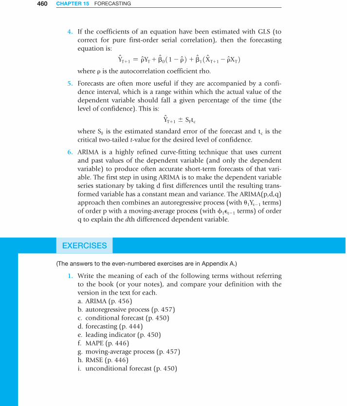
460 ChAPtER 15 Forecasting
4. If the coefficients of an equation have been estimated with GLS (to correct for pure first-order serial correlation), then the forecasting equation is:
YNT + 1 = ρNYT + βN 011 - ρN 2 + βN 11XN T + 1 - ρNXT2 where ρ is the autocorrelation coefficient rho.
5. Forecasts are often more useful if they are accompanied by a confi-dence interval, which is a range within which the actual value of the dependent variable should fall a given percentage of the time (the level of confidence). This is:
YNT + 1 ± SFtc
where SF is the estimated standard error of the forecast and tc is the critical two-tailed t-value for the desired level of confidence.
6. ARIMA is a highly refined curve-fitting technique that uses current and past values of the dependent variable (and only the dependent variable) to produce often accurate short-term forecasts of that vari-able. The first step in using ARIMA is to make the dependent variable series stationary by taking d first differences until the resulting trans-formed variable has a constant mean and variance. The ARIMA(p,d,q) approach then combines an autoregressive process (with θ1Yt - 1 terms) of order p with a moving-average process (with ϕ1et - 1 terms) of order q to explain the dth differenced dependent variable.
EXERCISES
(the answers to the even-numbered exercises are in appendix a.)
1. Write the meaning of each of the following terms without referring to the book (or your notes), and compare your definition with the version in the text for each.a. ARIMA (p. 456)b. autoregressive process (p. 457)c. conditional forecast (p. 450)d. forecasting (p. 444)e. leading indicator (p. 450)f. MAPE (p. 446)g. moving-average process (p. 457)h. RMSE (p. 446)i. unconditional forecast (p. 450)
M15_STUD2742_07_SE_C15.indd 460 1/16/16 12:36 PM

461ExErcisEs
2. Calculate the following unconditional forecasts:a. the median price (PR) of a new single-family house in 2014, given
the fact that the U.S. GDP in 2014 was roughly $17,400 billion and the following equation:
PRt = 12,928 + 17.08GDPt
b. the expected level of check volume at three possible future sites for new Woody’s restaurants, given Equation 3.4 and the following data. If you could only build one new eatery, in which of these three sites would you build (all else equal)?
Site Competition Population Income
Richburgh 6 58,000 38,000Nowheresville 1 14,000 27,000Slick City 9 190,000 15,000
3. To understand the difficulty of conditional forecasting, use Equa-tion 1.19 to forecast the weights of the next three males you see, using your estimates of their heights. (Ask for actual values after finishing.)
4. Some of the most interesting applications of econometric forecasting are in the political arena. Examples of regression analysis in politics range from part-time marketing consultants who help local candi-dates decide how best to use their advertising dollars to a fairly rich professional literature on U.S. presidential elections.13
In 2008, Haynes and Stone14 added to this literature with an article that specified (among others) the following equation:
VOTEi = β0 + β1Pi + β21DUR*P2i + β31DOW*P2i + β41GROWTH*P2i
+ β51INFLATION*P2i + β61ARMY*P2i + β71SPEND*P2i + ei
(15.20)
13. See, particularly, the work of Ray Fair: “The Effect of Economic Events on Votes for President,” Review of Economics and Statistics, Vol. 60, pp. 159–173, and “Econometrics and Presidential Elections,” Journal of Economic Perspectives, Vol. 10, pp. 89–102.
14. Stephen Haynes and Joe Stone, “A Disaggregate Approach to Economic Models of Voting in U.S. Presidential Elections: Forecasts of the 2008 Election,” Economics Bulletin, Vol. 4, No. 28 (2008), pp. 1–11.
M15_STUD2742_07_SE_C15.indd 461 21/01/16 1:59 PM

462 ChAPtER 15 Forecasting
where: VOTEi = the Democratic share of the popular two-party presidential vote
Pi = 1 if the incumbent is a Democrat and -1 if the incumbent is a Republican
DURi = the number of consecutive terms the incumbent party has held the presidency
DOWi = the annual rate of change in the Dow Jones Industrial Average between January and October of the election year
GROWTHi = the annual percent growth of real per cap-ita GDP in the second and third quarters of the election year
INFLATIONi = the absolute value of the annualized infla-tion rate in the two-year period prior to the election
ARMYi = the annualized percent change of the pro-portion of the population in the armed forces in the two-year period prior to the election
SPENDi = the annualized percentage change in the proportion of government spending devoted to national security in the two-year period prior to the election
a. What kind of variable is P? Is it a dummy variable? If not, what is it?b. The authors specified their equation as a series of interaction vari-
ables between P and the other variables of interest. Look at the equation carefully. Why do you think that these interaction vari-ables were required?
c. Using the data15 in Table 15.1 (datafile = ELECTION15) estimate Equation 15.20 for the years 1916–1996.
d. Create and test appropriate hypotheses on the coefficients of your estimated equation at the 5-percent level. Do any of the coefficients have unexpected signs? Which ones?
e. Create unconditional forecasts for the years 2000 and 2004 and compare your forecasts with the actual figures in Table 15.1. How did you do?
15. These data are from Haynes and Stone, ibid., p. 10, but similar tables are available from a variety of sources, including: fairmodel.econ.yale.edu/vote2008/pres.txt.
M15_STUD2742_07_SE_C15.indd 462 1/16/16 12:36 PM

463exercises
f. The authors wrote their article before the 2008 election. Create an unconditional forecast for that election using the data in Table 15.1. Who did the model predict would win? How did the model do?
Table 15.1 data for the presidential election exercise
YEAR VOtE P DUR DOW GROWth INFLAtION ARMY SPEND
1916 51.682 1 1 12.00 6.38 7.73 2.33 4.04
1920 36.119 1 2 -23.50 -6.14 8.01 -107.60 11.24
1924 41.756 -1 1 6.00 -2.16 0.62 -3.38 -23.05
1928 41.240 -1 2 31.30 -0.63 0.81 -0.48 10.15
1932 59.140 -1 3 -25.00 -13.98 10.01 -2.97 -37.56
1936 62.458 1 1 24.90 13.41 1.36 7.60 28.86
1940 54.999 1 2 -12.90 6.97 0.53 16.79 8.33
1944 53.774 1 3 9.00 6.88 1.98 53.10 17.16
1948 52.370 1 4 6.30 3.77 10.39 -38.82 -86.56
1952 44.595 1 5 -1.80 -0.34 2.66 43.89 71.59
1956 42.240 -1 1 2.40 -0.69 3.59 -9.93 -14.34
1960 50.090 -1 2 -13.90 -1.92 2.16 -4.10 -8.44
1964 61.344 1 1 15.80 2.38 1.73 -3.68 -5.88
1968 49.596 1 2 10.00 4.00 3.94 0.06 6.28
1972 38.210 -1 1 5.40 5.05 5.17 -11.91 -19.71
1976 51.050 -1 2 3.00 0.78 7.64 -2.56 -20.15
1980 44.697 1 1 12.40 -5.69 8.99 -1.37 -0.44
1984 40.830 -1 1 -6.90 2.69 3.68 -0.22 7.38
1988 46.070 -1 2 12.60 2.43 3.30 -1.58 -1.09
1992 53.455 -1 3 -0.90 1.34 3.15 -7.33 -10.11
1996 54.736 1 1 24.54 3.08 1.95 -5.62 -12.67
2000 50.265 1 2 -5.02 2.95 1.80 -2.00 1.83
2004 48.586 -1 1 -8.01 3.49 2.50 -0.51 14.91
2008 ? -1 2 30.70 2.10 3.70 -0.87 0.41
source: stephen haynes and Joe stone, “a disaggregate approach to economic Models of Voting in u.s. presidential elections: Forecasts of the 2008 election,” Economics Bulletin, Vol. 4, no. 8 (2008), p. 10.
datafile = election15
M15_STUD2742_07_SE_C15.indd 463 1/16/16 12:36 PM

464 ChAPtER 15 Forecasting
5. Suppose you have been given two different ARIMA (1,0,0) fitted time-series models of the variable Yt:
Model A: Yt = 15.0 + 0.5Yt - 1 + et
Model T: Yt = 45.0 - 0.5Yt - 1 + et
where et is a normally distributed error term with mean 0 and stan-dard deviation equal to 1.a. The final observation in the sample (time period 06) is Y06 = 31.
Determine forecasts for periods 07, 08, and 09 for both models.b. Suppose you now find out that the actual Y07 was equal to 33.
Revise your forecasts for periods 08 and 09 to take the new infor-mation into account.
c. Based on the fitted time series and your two forecasts, which model (model A or model T) do you expect to exhibit smoother behavior? Explain your reasoning.
M15_STUD2742_07_SE_C15.indd 464 1/16/16 12:36 PM