crooked volatility smiles: evidence from leveraged … article crooked volatility smiles: evidence...

Original Article

Crooked volatility smiles: Evidence from leveraged

and inverse ETF optionsReceived (in revised form): 7th January 2014

Geng Deng

is the Director of Research at Securities Litigation and Consulting Group, Inc. He specializes in the fields ofderivatives, credit modeling, structured finance, mutual fund and hedge fund investment analysis. He holds aPhD in Operations Research, an MA in Mathematics and an MS in Statistics, all from the University of Wisconsin–Madison. He also holds a BS in Applied Mathematics from Tsinghua University in China. He was the recipient ofseveral best paper awards when he was in graduate school. He holds a Financial Risk Manager (FRM)designation and is a CFA® charterholder.

Tim Dulaney

is a senior financial economist at Securities Litigation and Consulting Group (SLCG). He earned a PhD inTheoretical Physics from the California Institute of Technology, specializing in early Universe cosmology andparticle physics. He graduated Summa Cum Laude and Phi Beta Kappa from the University of Maryland with a BSin Mathematics with High Honors and a BS in Physics with High Honors. At SLCG, he has analyzed and valuedcomplex financial products such as fixed and indexed annuities, interest rate swaps, options, structured productsincluding structured CDs, and exchange-traded products.

Craig McCann

has extensive experience in securities class action litigation, financial analysis, investment management andvaluation disputes. Prior to founding the Securities Litigation and Consulting Group, he was Director at LECG andManaging Director, Securities Litigation at KPMG. He was a senior financial economist at the Securities andExchange Commission, where he focused on investment management issues and contributed financial analysisto numerous investigations involving alleged insider trading, securities fraud, personal trading abuses and broker–dealer misconduct. In addition, he is a CFA® charterholder.

Mike Yan

is a senior financial economist at Securities Litigation and Consulting Group, Inc. He holds a PhD in AppliedMathematics from the University of California at Davis. He specializes in the fields of applied mathematics,including stochastic analysis, ordinary/partial differential equations, time series analysis, statistics and probability.His doctoral work focused on the stability and resolution analysis in imaging science. He also taught severalnumerical analysis courses when he served as von Karman Instructor of Applied and Computational Mathematicsat the California Institute of Technology.

Correspondence: Geng Deng, Securities Litigation and Consulting Group, Inc., 3998 Fair Ridge Drive, Suite 250,Fairfax, VA 22033, USAE-mail: [email protected]

ABSTRACT We find that leverage in exchange traded funds (ETFs) can affect the ‘crook-edness’ of volatility smiles. This observation is consistent with the intuition that returnshocks are inversely correlated with volatility shocks – resulting in more expensive out-of-the-money put options and less expensive out-of-the-money call options. We show that theprices of options on leveraged and inverse ETFs can be used to better calibrate models of

© 2013 Macmillan Publishers Ltd. 1753-9641 Journal of Derivatives & Hedge Funds Vol. 19, 4, 278–294www.palgrave-journals.com/jdhf/

stochastic volatility. In particular, we study a sextet of leveraged and inverse ETFs based onthe S&P 500 index. We show that the Heston model can reproduce the crooked smilesobserved in the market price of options on leveraged and inverse leveraged ETFs. We showfurther that the model predicts a leverage-dependent moneyness, consistent with empiricaldata, at which options on positively and negatively leveraged ETFs (LETF) have the sameprice. Finally, by analyzing the asymptotic behavior for the implied variances at extremestrikes, we observe an approximate symmetry between pairs of LETF smiles empiricallyconsistent with the predictions of the Heston model.

Journal of Derivatives & Hedge Funds (2013) 19, 278–294. doi:10.1057/jdhf.2014.3

Keywords: exchange traded funds (ETFs); leveraged ETFs; stochastic volatility; volatility smiles;options

INTRODUCTION

Empirical motivation

By relating option prices to observables (suchas strike prices, time-to-expiration, spot priceand so on) and one unknown parameter(implied volatility of the underlying asset returndynamics), Black and Scholes (1973) allowedpractitioners to more systematically studyobserved option prices. Furthermore, thisunknown parameter allowed researchers tonormalize comparisons between options withdifferent observables.For all of the success of the Black-Scholes

model and for its near-ubiquity today, there areseveral shortcomings of the model. For example,Rubinstein (1985) pointed out strike price biasesand close-to-maturity biases by studying theprices of the most active option on the CBOE.1

In subsequent works, Rubinstein (1994) andJackwerth and Rubinstein (1996) showed thatoptions on stocks and stock options exhibitvolatility skew and that foreign currency optionsexhibit a volatility smile (at-the-money optionsare cheaper than in-the-money or out-of-the-money options).

In Figure 1, we show a typical volatility smilefor call options on equities and equity indices.2

The volatilities implied by the prices of in-the-money options is higher than the volatilityimplied by the prices of at-the-money optionswhich is higher than the volatility implied bythe prices of out-of-the-money options.In this article, we study the implied volatility

surface of options on leveraged ETFs (LETFs)and inverse leveraged ETFs (ILETFs). Inparticular, we consider members of a sextet ofexchange traded funds (ETFs) tracking the S&P500 index. See Table 1 for the names, tickers andcorresponding leverage factor (ℓ ).The dailypercentage change in the net asset value of anETF with leverage factor ℓ is ℓ times the dailypercentage change of the underlying index.3

LETFs have leverage factor ℓ⩾1, whereasILETFs have leverage factor ℓ⩽−1.4

According to the Black-Scholes model, anoption on an LETF with leverage factor ℓ⩾1should have the same price as an option on anILETF with leverage factor (−ℓ ) if both optionsshare the same strike price and expiration – ifthese ETFs share the same underlying index.5

This is intuitive because, in risk-neutral

Crooked volatility smiles

279© 2013 Macmillan Publishers Ltd. 1753-9641 Journal of Derivatives & Hedge Funds Vol. 19, 4, 278–294

valuation, the only difference between theevolution of the LETF or ILETF is the leveragefactor that proportionally increases the volatility.Since the option price is dependent on the squareof the volatility, the price of options on LETFsand ILETFs with the same strike and expirationshould have the same price.In Figure 2(a), we show the volatility smile for

options on an LETF with ℓ= 3 and an ILETFwith ℓ=−3. The pattern of implied volatilitiesfor ProShares UltraPro S&P 500 ETF (UPRO) issimilar to the pattern of implied volatilies inFigure 1(a), with the volatilities of UPROroughly three times the implied volatilities fromoptions on SPY. On the other hand, the optionson the inverse ETF (SPXU) have impliedvolatilities that are a decreasing function of the

moneyness. Figure 2(a) shows that the predictionof the option prices under the Black-Scholesmodel is not consistent with empirical data.Figure 2(b) shows the price of call options

on these LETFs as a function of the normalizedstrike price. These observations suggest that thecrookedness of the volatility smile is dependenton the leverage factor ℓ.The prices of in-the-money call options on

positively LETFs (ℓ1⩾1) imply lower volatilitiesthan the prices of in-the-money call options onILETFs (ℓ2⩽0) for the same level of leverage(ℓ1= |ℓ2|) and moneyness. Similarly, the prices ofout-of-the-money call options on positivelyLETFs imply lower volatilities than the prices ofout-of-the-money call options on ILETFs forthe same level of leverage and moneyness.6

Intuitively, we expect stock returns to benegatively correlated with volatility shocks – forexample, large price decline and an increase involatility. As a result, far from the money putoptions are more expensive than one may naivelyexpect. As a result, the volatility implied byoption market prices is increasing with decreasingmoneyness, as shown in Figure 2(a). For aninverse ETF, stock returns would be positivelycorrelated with volatility shocks – for example,large price declines in the underlying lead to largeprice increases in the inverse ETF. As a result, the

15%

20%

25%

30%

90% 95% 100% 105% 110%

Imp

lied

Vo

lati

lity

Strike Price/Asset Price

a b

0%

5%

10%

15%

90% 95% 100% 105% 110%

Op

toin

Prc

e/A

sset

Pri

ce


Figure 1: Market observed (a) implied volatilities and (b) market prices of 3-month call options

on SPDR S&P 500 ETF (SPY) on 19 October 2009.

Table 1: Sextet of LETFs tracking the S&P 500

index

Fund name Ticker ℓ

ProShares UltraPro Short S&P 500 ETF SPXU −3ProShares UltraShort S&P 500 ETF SDS −2ProShares Short S&P 500 ETF SH −1SPDR S&P 500 ETF SPY 1ProShares Ultra S&P 500 ETF SSO 2ProShares UltraPro S&P 500 ETF UPRO 3

Deng et al

280 © 2013 Macmillan Publishers Ltd. 1753-9641 Journal of Derivatives & Hedge Funds Vol. 19, 4, 278–294

volatility implied by option market prices oninverse ETFs should be increasing with increasingmoneyness. The combination of these twoarguments implies that low moneyness optionson positively LETFs will be more expensive thansimilar options on negatively LETFs.We explore this phenomenon, as well as the

crossing phenomena shown in Figure 2(b), bothempirically and theoretically in this article.7

Although this phenomenon is intuitive, therehas been no study of the crossing behaviordepicted in Figure 2(b) and this article seeks tofill this gap.

Observable implications

We use the stochastic volatility model in Heston(1993) to explain the ‘crooked smiles’ in theoptions market. This Heston model, similar tothe Black-Scholes model, has closed-formsolutions for the valuation of European put andcall options but incorporates stochastic volatility.Unlike the constant implied volatility in the

Black-Scholes model, the dynamics of thevolatility is correlated with the dynamics of thestock price or index level in the Heston model.This stochastic volatility model is better equipped

to account for observed skewness and kurtosis ofreturn distributions.8

Volatility smiles have often been explainedeither by jump-diffusion models as suggested byMerton (1976) or with stochastic volatility as inmodels proposed by Hull and White (1987) andHeston (1993). We consider the Heston modelhere because of the convenient analyticproperties.Option pricing in the context of LETFs has

recently gained interest in the literature. Ahnet al (2012) and Zhang (2010) use standardtransformation methods to price options on ETFsand LETFs within the Heston stochastic volatilityframework. We extended their research byderiving the dynamics of LETFs. The closed-form solutions use a Green function approachfollowing the method in Lipton (2001). Ournumerical simulations show that the Hestonmodel can explain the patterns in option priceson LETFs and ILETFs. We observe that thecrooked smile is present only when there existsnon-zero correlation between the Brownianmotions for the asset returns and the variance.9

Furthermore, we show that the model predicts amoneyness – dependent on the level of leverage– for which the prices of positively and negatively

45%

60%

75%

90%

75% 95% 115% 135% 155% 175%

Imp

lied

Vo

lati

lity


a bSPXU (l = -3) UPRO (l = 3)

0%

5%

10%

15%

20%

25%

30%

75% 95% 115% 135% 155% 175%

Op

tio

n P

rice

/Ass

et P

rice


SPXU (l = -3) UPRO (l = 3)

Figure 2: Market observed (a) implied volatilities and (b) market prices of 3-month call options

on ProShares UltraPro Short S&P 500 ETF (SPXU) and ProShares UltraPro S&P 500 ETF

(UPRO) for different strike prices on 19 October 2009.



LETF options have the same price and that thisprediction is consistent with empirical data.We also study the asymptotic behavior of

implied variance curves for options on LETFand ILETF. This analysis relies heavily on themoment expansion framework in Lee (2004) andRollin et al (2009). Subsequent analyses – Frizet al (2011) and de Marco and Martini (2012) –refined the volatility smile expansion within theHeston model. Building on Lee’s work, Benaimand Friz (2009) showed how the tail asymptoticsof risk-neutral returns can be directly related tothe asymptotics of the volatility smile and theyapplied this approach to time-changed Lévymodels and the Heston model (Benaim and Friz,2008).We provide empirical evidence that the

asymptotic slopes of the implied variance curvesfor options on LETF and ILETF show anapproximate symmetry and that this approximatesymmetry is consistent with the Heston model.In particular, we show that the large-strikeasymptotic slopes of the implied variancecurves for LETFs are related to the small-strikeasymptotic slopes of the implied variance curvesfor ILETFs. Both simulated examples and marketdata are presented.The rest of the article is organized as

follows: In the second section, we review theBlack-Scholes model and Heston stochasticvolatility model. The closed-form solution ofthe call options of LETF and ILETF is derivedunder Heston dynamics. In the third section,the asymptotic behaviors of the option pricesare studied as the moneyness goes extremelylarge and small. In the fourth section, wesimulate the option prices under Hestondynamics, and compare the prices acrossdifferent leverage numbers ℓ. In addition, wecalibrate our model using the empirical data in

the fifth section. The article is concluded in thesixth section.

LEVERAGED AND INVERSE ETF

OPTION PRICES

The Black-Scholes model

If an asset price St follows a geometric Brownianmotion then its dynamics are described by theclassic stochastic differential equation

dStSt

¼ ðμ - qÞdt + σdWt;

where μ, q and σ are expected return, dividendyield and implied volatility of the asset,respectively. All three parameters are assumedto be constant and continuously compounded.The price of an LETF or ILETF Lt, whichtracks ℓ times daily return of the underlying asset,satisfies

dLt

Lt¼ ðμ‘ - q‘Þdt + σ‘dWt:

where μℓ=ℓμ and σℓ=ℓσ. This implies that thevolatilities of the returns are leveraged |ℓ | times.Under risk-neutral assumptions, the expected

return of the LETFs μl is the risk-free rate r,independent of ℓ. Therefore, the option priceC(t, L) satisfies the following Black-Scholesequation:10

∂C∂t

+12σ2‘2L2 ∂

2C∂L2

+ ðr - q‘ÞL ∂C∂L

- rC ¼ 0; (1)

where r is the constant risk-free rate.In this model, the volatility (the standard

deviation for the instantaneous ETF returndLt/Lt) is always |ℓ |σ, and is independent of thestrike price of the option contract, as well as thesign of the leverage number ℓ. If both LETF andILETF have the same leverage factor in absolutevalue and the same dividend yield qℓ, we shouldobserve the same implied volatility and same

Deng et al


option price under the Black-Scholes model.Figure 2(b) shows that this theoretical predictionis inconsistent with observed market optionprices.

Heston’s stochastic volatility model

Since the Black-Scholes model is not able toadequately describe the phenomena observed inthe option prices on the sextet of LETFs in thesection ‘The Black-Scholes Model’, we turn toalternative models of asset dynamics. We chooseto discuss the Heston model (Heston, 1993) inparticular because of the closed-form solutionsfor European option prices and the depth ofliterature analyzing the details of the model.In the risk-neutral framework, we write Lt as

the price of the LETF or ILETF, vt as the varianceof the underlying stock. These variables aregoverned by the dynamics

dLt

Lt¼ ðr - q‘Þdt + ‘ ffiffiffiffi

vtp

dW1t; (2)

dvt ¼ κðθ - vtÞdt + ε ffiffiffiffivt

pdW2t: (3)

where W1t and W2t are two Brownian motionswith a correlation value ρ, that is,

E dW1tdW2t½ � ¼ ρdt (4)

A simple derivation shows that the stochasticprocess Lt is linked to the underlying stock priceprocess St and the realized variance ∫0tvtdt

Lt

L0¼ St

S0

� �‘

exp‘ - ‘2

2

Zt0

vsds + ð1 - ‘Þr0@

1A (5)

The equation implies that a higher realizedvariance implies a larger deviation between theholding period returns of LETFs and those of theunderlying stock. Although the equation cannotbe directly used in valuing options on LETFs, itshows the necessity of using stochastic volatility

models since dynamic variance is an importantcomponent of the return of LETFs.11

Utilizing the following theorem, we derive thecall option value for LETFs.

Theorem 1 The value of an European calloption with strike K for an LETF in theHeston model is in the form

CðLt; v0; τÞ ¼ KeXt2 - rτUðτ;Xt; v0Þ; (6)

where v0 is the initial variance value at time0 and τ is the time to maturity τ=T−t. Xt isdefined as ln(Ft)/(K), where Ft is the for-ward price of LETF and is defined as Ft=Lte

(r−q)τ. The function U(τ,Xt, v0) is givenby equation (A.6) in Appendix.

Proof: See proof in Appendix. □Alternatively, a single set of change variables

could simplify the valuation approach. If weintroduce the following change of variables12

v̂t ¼ ‘2vt;

θ̂ ¼ ‘2θ;

ε̂ ¼j ‘ j ε;ρ̂ ¼ Signð‘Þρ; ð7Þ

The stochastic differential equations inequation (2) and equation (3) are converted intothe following standard Heston model

dLt

Lt¼ ðr - qÞdt +

ffiffiffiffiv̂t

pdW1t; (8)

dv̂t ¼ κðθ̂ - v̂tÞdt + ε̂ffiffiffiffiv̂t

pdW2t: (9)

Note that the new equations are free of theleverage factor ℓ thus we can use the Liptonsolution or Heston solution given ℓ= 1. Havingderived the dynamics of leveraged and inverseETFs based on the dynamics of the underlyingindex, we move on to consider the pricing ofoptions on leveraged and inverse ETFs.



SYMMETRY IN IMPLIED

VARIANCES FOR LETF OPTIONS

In this section, we study the implications ofAndersen and Piterbarg (2007) to the extremestrike behavior of option prices on leveraged andinverse ETFs.13 Our results build heavily on thework by Lee (2004), wherein the author showedthat the extreme strike behavior is related to thenumber of finite moments of the returndistribution.14

In particular, at large strikes the Black-Scholesimplied variance becomes a linear function of thelogarithm of the strike price. Lee (2004) showedthat the small-strike asymptotic behavior is also alinear function of the logarithm of the strike priceusing the properties of the inverse price process.Following Friz and Keller-Ressel (2009), a

model is said to exhibit moment explosion atorder α>1 if there exists some finite T*(α)such that E SαT *

� � ¼ 1. The time of momentexplosion T*(α) depends on the moment underconsideration and is the smallest time such thatE[St

α ]<∞. If, for some β, E[Stβ ] is finite for all t

then T*(β)=∞.Lee (2004) showed that the large-strike

(K≫F0) Black-Scholes implied variance isrelated to the degree of moment explosionthrough the following theorem.15

Theorem 2 If p*= sup{p|E[ST1+p]<∞} and

βR= limsupx→∞(σBS2 (x))/(|x|/T), then

βR ¼ 2 - 4ffiffiffiffiffiffiffiffiffiffiffiffiffiffiffiffiffiffiffip*ðp* + 1Þ

p- p*

� �(10)

Lee (2004) showed further that the extremesmall-strike (K≪F0) asymptotic behavior of theBlack-Scholes implied volatility can be relatedto the degree of moment explosion of theinverse price process through the followingtheorem.

Theorem 3 If q*= sup{q|E[ST−q]<∞} and

βL= lim supx→∞(σBS2 (x))/(|x|/T), then

BL ¼ 2 - 4ffiffiffiffiffiffiffiffiffiffiffiffiffiffiffiffiffiffiffiq* q* + 1ð Þ

p- q*

� �: (11)

When βL or βR is 0, the underlying modeldoes not exhibit moment explosion. Note thatp*= α+

*−1, where α+* is the degree of moment

explosion or the critical moment for the processSt at time T and q*= α−

* , where α−* is the critical

moment for the inverse price process ST−1 at

time T.Andersen and Piterbarg (2007), in their

Proposition 3.1, show how to relate the degree ofmoment explosion α+ to the parameters in theHeston model as well as the time of momentexplosion T*(α+). Following Corollary 6.2 inAndersen and Piterbarg (2007), the criticalmoment α+

* is obtained by solving T*(α+)=T.To solve the critical moment α−

* for the inverseprice process, Rollin (2008) showed that if anasset follows a price process described by theHeston model then the inverse spot price followsa price process described by the Heston modelwith the following parameters

~κ ¼ κ - ρε; ~ρ ¼ - ρ and ~θ ¼ κθ=~κ (12)

where the parameters f~κ; ~θg represent theanalogous parameters in the inverse spot priceprocess to those in the non-inverted price process.Using these results, we can study the symmetry ofBlack-Scholes implied variances at extreme strikesfor options on LETFs and ILETFs.Referring to the parameter translations in

equation (7), we see that the LETF price processLt, ℓ is closely linked to the inverse of the ILETFprice process Lt,−ℓ, Lt, ℓ≈Lt, ℓ−1 . The followingtable shows the corresponding parameters usedfor the two price processes when we combine theresults in equation (7) with the result in equation(12) (Table 2).

Deng et al


The Heston model parameters v̂t, ε̂ and ρ̂ arethe same for both processes. In practice, theHeston model parameters κ̂ and θ̂ are not exactlythe same, but they are close. Therefore, thecritical moments for the LETF price process α*+, ℓapproximates the critical moment for the inverseof ILETF process α*−,−ℓ. The theorems abovepredict that βR, ℓ≈ βL,−ℓ. In other words, theratio of the Black-Scholes implied variance to themoneyness of deep-in-the-money call optionson LETFs equals the ratio of the Black-Scholesimplied variance to the moneyness of deep-out-of-the-money call options on ILETFs of the sameleveraged amplitude. The asymmetry betweenthese two slopes is related to the volatility ofvariance (ϵ) and increases approximately linearlywith the degree of leverage for small values of thevolatility of variance. In the fourth and fifthsections, we will give two examples of criticalmoments and asymptotic slopes highlighting therelationships.

NUMERICAL SIMULATIONS

Simulation parameters

In this section, we present numerical simulationsto show the dependence of the leverage-skew on

model parameters. By studying this dependence,we can hope to endow the reader with anunderstanding of the patterns predicted by theHeston model. For our numerical simulations,we fix the following parameters

Initial volatility : v0 ¼ ð15% Þ2;Riskfree interest rate : r ¼ 2% ;

Dividend yield : q ¼ 1% ;

Variancemeanreversion rate : κ ¼ 2;

Longterm variance : θ ¼ ð15% Þ2;Volatility of variance : ε ¼ 0:1;

Time : T ¼ 0:5;

Initial stock price : S0 ¼ 100:

In what follows, we vary the correlation ρ

between returns and return variance, the leveragenumber ℓ, and the strike price K (or equivalently,the moneyness). By varying these parameters,we analyze the model and explain the patternimplied by market prices of options on leveragedand inverse ETFs. The model calibration on theempirical data will be discussed in the fifthsection.In Figure 3, we vary the strike price of the call

option and show the call option price for eachleverage number in {−3,−2,−1, 1, 2, 3} keepingthe correlation fixed at ρ=−0.5. The call optionprices are seen to be split into pairs, with theprices of the doublets {−ℓ, ℓ} being comparable.The Heston model with the current set of

parameters is ready to explain the volatility smile.Hull (2011) shows that the call option prices are amonotone increasing functions of the impliedvolatility. Hence, the higher the impliedvolatility, the higher the call option price.

Break-even strike prices

Call options that are deep-in-the-money, that is,K≪ S0 on the LETF with leverage number ℓ> 0

Table 2: Comparing the parameters used in

the Heston model for the LETF price process

Lt, ℓ and the inverse of ILETF price process Lt, −ℓ−1

Parameters Lt, ℓ Lt,−ℓ−1

v̂t ℓ2vt ℓ2vtε̂ |ℓ|ϵ |ℓ|ϵρ̂ Sign(ℓ)ρ −Sign(ℓ)ρκ̂ κ κ−ℓρε

θ̂ ℓ2θ ℓ2θκ/κ−lρε



are more expensive than the same-strike calloptions on the ILETF with leverage number −ℓ.For options that are deep-out-of-the-money(K≫S0), the conclusion reverses: the optionprices on the ILETF are more expensive than thaton the LETFs.16 These simulated curves are verysimilar to what we have observed in Figure 3(b).Both simulated and empirical curves imply thatthere exists a critical (or ‘break-even’) strike price(K*(|ℓ|)) at which the call option price of a LETFwith leverage number ℓ>0 equals the call optionprice on a ILETF with leverage number −ℓ.Table 3 reports those critical strike prices thatresults in equality between the prices of optionson LETFs and ILETFs within the same doublet(ℓ=±|ℓ |) for our numerical simulations. In thisparticular set of parameters, the break-even strikeprice/moneyness decreases as the leverage factorincreases.Table 3 demonstrates the dependence of the

break-even prices on the leverage |ℓ |. In Figure 4,we plot the difference between call option priceson the LETF and ILETF within the same doubletfor different values of the correlation coefficient ρ.This set of graphs shows that the price differenceof the call options is symmetric with respect to ρ.

The simulations further show that the break-evenstrike prices, when the option price differencesequal zero, are independent of ρ.Figure 4 make a few aspects of the phenomena

predicted by this model clear.

● If the correlation coefficient is 0, the differencebetween the call option prices is 0. In this case,the changes in the volatility are independentof the changes in the stock price. Hence theHeston model essentially becomes a Black-Scholes model with implied volatility beingthe expected mean volatility in the Hestonmodel.

70 80 90 100 110 120 1300

5

10

15

20

25

30

35a b

Strike Price K

Cal

l Opt

ion

Pric

e

70 80 90 100 110 120 1300.1

0.15

0.2

0.25

0.3

0.35

0.4

0.45

0.5

Strike Price K

Impl

ied

Vol

atili

ty

=−3=−2=−1=1=2=3

=−3=−2=−1=1=2=3

Figure 3: Simulated (a) call option prices and (b) implied volatilities with different strike price

K, different leverage number ℓ and correlation ρ=−0.5.

Table 3: Summary of the break-even strike

prices that lead to the same option values

for leveraged ETFs within the same doublet

(ℓ=±|ℓ |). For these simulations, we use

ρ=−0.5

Leverage number K*(|ℓ |)(in dollars)

Option price(in dollars)

ℓ=±1 99.944 4.459ℓ=±2 98.289 9.414ℓ=±3 95.592 14.794

Deng et al


● As ℓ increases, the difference between theprices of options on LETF and ILETF increasesin magnitude. That can be partially explainedthat the higher volatility of the leverage funds,the higher option premium.

● Upon changing the sign of ρ, the cheaperoption becomes the more expensive option forfixed strike within the same doublet of ETFs.17

● The break-even strike price within each doubletis independent of ρ. Although we present only ahandful of correlation examples in Figure 4, thisconclusion holds for all values of ρ.

Note that deep-out-of-the-money call optionson ILETFs are more expensive than deep-out-of-the-money call options on LETFs when ρ<0.If the correlation coefficient ρ is negative, the

volatility and the price of ILETF tend to increasesimultaneously. With the same parameters, theprice of LETF increases, while the volatility tendsto decrease. Intuitively, the ILETF option has ahigher probability of ending in-the-money thanthe analogous LETF. As a result, the call optionprices on an ILETF with high strike are oftenmore expensive than call option prices on anLETF when stock price and implied volatility arenegatively correlated.

Asymptotic implied variance slope

We explore the correspondence present betweenhigh-strike asymptotic behavior of positivelyLETFs and low-strike asymptotic behavior ofnegatively LETFs in Table 4. In this context, it is

60 80 100 120−0.1

−0.05

0

0.05

0.1

= ±1

= ±3

60 80 100 120−0.1

−0.05

0

0.05

0.1

= ±2

60 80 100 120−0.1

−0.05

0

0.05

0.1� =−1

� =−0.5

� =0

� =0.5

� =1

Relative Call Option Price Difference of LETF and ILETF

Figure 4: Difference between call option prices for leveraged and ILETFs within the same

doublet, for different values of the correlation coefficient ρ as a function of the strike price of

the option contracts. The option contracts in this figure are normalized so that initial stock

price S0= 100.



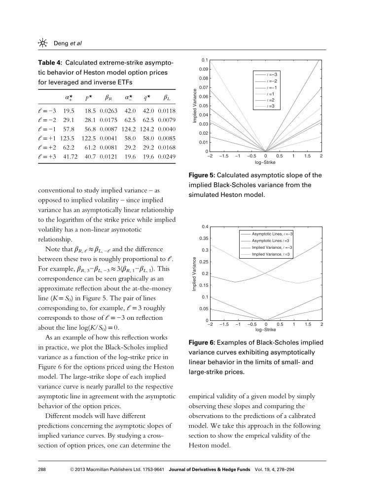
conventional to study implied variance – asopposed to implied volatility – since impliedvariance has an asymptotically linear relationshipto the logarithm of the strike price while impliedvolatility has a non-linear asymototicrelationship.Note that βR, ℓ≈ βL,−ℓ and the difference

between these two is roughly proportional to ℓ.For example, βR, 3−βL,−3≈ 3(βR, 1−βL, 1). Thiscorrespondence can be seen graphically as anapproximate reflection about the at-the-moneyline (K= S0) in Figure 5. The pair of linescorresponding to, for example, ℓ= 3 roughlycorresponds to those of ℓ=−3 on reflectionabout the line log(K/S0)= 0.As an example of how this reflection works

in practice, we plot the Black-Scholes impliedvariance as a function of the log-strike price inFigure 6 for the options priced using the Hestonmodel. The large-strike slope of each impliedvariance curve is nearly parallel to the respectiveasymptotic line in agreement with the asymptoticbehavior of the option prices.Different models will have different

predictions concerning the asymptotic slopes ofimplied variance curves. By studying a cross-section of option prices, one can determine the

empirical validity of a given model by simplyobserving these slopes and comparing theobservations to the predictions of a calibratedmodel. We take this approach in the followingsection to show the emprical validity of theHeston model.

Table 4: Calculated extreme-strike asympto-

tic behavior of Heston model option prices

for leveraged and inverse ETFs

α*+ p* βR α*− q* βL

ℓ=−3 19.5 18.5 0.0263 42.0 42.0 0.0118ℓ=−2 29.1 28.1 0.0175 62.5 62.5 0.0079ℓ=−1 57.8 56.8 0.0087 124.2 124.2 0.0040ℓ=+1 123.5 122.5 0.0041 58.0 58.0 0.0085ℓ=+2 62.2 61.2 0.0081 29.2 29.2 0.0168ℓ=+3 41.72 40.7 0.0121 19.6 19.6 0.0249 −2 −1.5 −1 −0.5 0 0.5 1 1.5 2

0

0.01

0.02

0.03

0.04

0.05

0.06

0.07

0.08

0.09

0.1

log−Strike

Impl

ied

Var

ianc

e

=−3=−2=−1=1=2=3

Figure 5: Calculated asymptotic slope of the

implied Black-Scholes variance from the

simulated Heston model.

−2 −1.5 −1 −0.5 0 0.5 1 1.5 20

0.05

0.1

0.15

0.2

0.25

0.3

0.35

0.4

log−Strike

Impl

ied

Var

ianc

e

Asymptotic Lines, =−3

Asymptotic Lines =3

Implied Variance, =−3

Implied Variance, =3

Figure 6: Examples of Black-Scholes implied

variance curves exhibiting asymptotically

linear behavior in the limits of small- and

large-strike prices.

Deng et al


EMPIRICAL OPTIONS DATA

In the previous section, we relied on simulateddata to test the Heston model’s sensitivity tomodel parameters. In this section, we calibrateour model to options data for all LETFs andILETFs listed in Table 1.There are five parameters to calibrate: mean

reversion rate κ, long-term variance θ, volatilityof variance ϵ, correlation ρ and initial volatility v0.Since all the ETFs track the same underlyingindex, their underlying processes are relatedthrough the leverage factor ℓ. The five unknownparameters to be calibrated are thereforecommon to all members of the sextet.We follow the most common approach in the

option pricing calibration literature and minimizethe difference between observed option pricesand Heston model option prices:18

minκ;θ;ϵ;ρ;v0

X‘;T

ωT ;‘

Cð‘ÞT ;market � Cð‘Þ

T ;model

Lð‘Þ0

!28<:

9=;

1=2

(13)

with the weight function ωT, l. Since the calloptions values are proportional to the initialprice L0

ℓ for each ETF, we normalize the absolutedifference of the market price and the modelprice by dividing by the initial LETF price.Other calibration approaches have been proposedaccording to the one-to-one relationshipbetween the option price and the impliedvolatility. Instead of fitting the option pricesdirectly, one could fit the model volatility/variance to the market volatility/variance impliedby the Black-Scholes model in the least squaresense (see Kjellin and Lövgren, 2006). For thecurrent article, we discuss the optimizationproblem in equation (13) with equal weightωT, l= 1.

Using the procedure outlined above, wesolved for the model parameters for over 100trading days between July and December 2009.The best-fit parameters varied each day, but over90 per cent of the days have a volatility ofvariance parameter (ε) in the range [0.5, 3.5]and a correlation parameter ( ρ) in the range[−0.45,−0.75].As an example, we again focus on the LETF

option data as of 19 October 2009. Theoptimization procedure is implemented inMATLAB using the routine lsqnonlin. Mostoptimization procedures are very efficient andrequire less than 200 function evaluations.Since in-the-money call options on

negatively LETFs have higher prices than thesame option on a positively LETFs, we expectthe correlation between the asset price andvariance to be negative. Indeed, our resultsindicate the best-fit value for the correlationis −0.565.Since our model uses more options data

(option data over a sextet of LETFs), thecalibrated parameters are more preciselydetermined and stable when compared to acalibration using only options on the unleveragedmember of the sextet (SPY, ℓ= 1).Given the calibrated model parameters in

Table 5, we can compute the asymptoticbehavior of the implied variance curves. Theresults of this computation are summarized inTable 6.

Table 5: Heston model calibration using

market prices of options on the sextet of

LETFs and ILETFs

κ θ ϵ ρ ν0

6.8791 0.0669 1.3357 −0.5649 0.0359



The difference between βR(ℓ) and βL

(−ℓ) is morepronounced here than in Table 4 as a result of thevolatility of variance ε. This calibrated parameterε is more than 10 times larger than that used forthe numerical simulations in the fourth section.We plot the implied variance curves of themarket prices as well as the asymptotic impliedvariance lines in Figure 7 for SPXU (ℓ=−3) andUPRO (ℓ=+3).The variance implied by the market prices

of options on UPRO and SPXU are plotted inbold in Figure 7. The asymptotic behavior ofthese empirical curves is explained by the calibratedHeston model.

CONCLUSION

This article was motivated by the empiricalobservations of robust and persistent crookedsmiles implied by the option prices on LETFs andILETFs. In particular, we note that deep-in-the-money call options on the LETF with leveragenumber ℓ>0 are more expensive than calloptions with the same moneyness and expirationon the ILETF with leverage number −ℓ. Since

the Black-Scholes model cannot properly explainthis phenomena, we turn to the Heston stochasticvolatility model. Since the call option price ofHeston model is given explicitly, it is convenientto analyze the Heston model than otherstochastic volatility model, which in general needMonte Carlo simulations. Following Lipton(2001), we derived the option values of LETFsand ILETFs with the same underlying via theGreen’s function approach. Here we used oneimportant fact that the dynamics of LETFs andILETFs with the same underlying index haverelated dynamics.We gathered pricing data for LETF options

on the sextet of ETFs (ℓ∈{−3,−2,−1, 1, 2, 3})with the S&P 500 as the underlying index. Weshowed that the Heston model can reproduce thecrooked smiles observed in the empirical dataand, using numerical simulations, showed howdifferent phenomena in the options data couldbe produced with different model parameters.

Table 6: Calculated extreme-strike asympto-

tic behavior of Heston model after calibration

to market prices of options on the sextet of

ETFs with the S&P 500 as the underlying

index on 19 October 2009

α*+ p* βR α*− q* βL

ℓ=−3 3.510 2.510 0.1672 9.246 9.246 0.0513

ℓ=−2 5.055 4.055 0.1101 13.348 13.348 0.0361

ℓ=−1 9.710 8.710 0.0543 25.679 25.679 0.0191

ℓ=+1 24.711 23.711 0.0207 9.973 9.973 0.0478

ℓ=+2 12.862 11.862 0.0405 5.185 5.185 0.0881

ℓ=+3 8.919 7.919 0.0594 3.597 3.597 0.1225

−2 −1.5 −1 −0.5 0 0.5 1 1.5 20

0.2

0.4

0.6

0.8

1

1.2

1.4

1.6

1.8

log−Strike

Impl

ied

Var

ianc

e

Asymptotic Lines, = −3

Asymptotic Lines =3

Implied Variance, = −3

Implied Variance, =3

SPXU Implied Variance

UPRO Implied Variance

Figure 7: Examples of Black-Scholes implied

variance curve for the market prices of

options on SPXU and UPRO (ℓ=±3) on 19

October 2009 and the asymptotic behavior of

these curves implied by the calibrated

Heston model.

Deng et al


In particular, we studied the asymptotic behaviorof Black-Scholes implied volatility curves andcompared these to the predictions given by theHeston model calibrated to the market prices ofoptions.An important contribution of this article is

that using options data of LETFs and ILETFs inaddition to options data on the underlyingindex itself can better calibrate the pricingdynamics of the index. Using the closed-formsolutions for the option prices of LETFs andILETFs derived in this article, practitioners canmore effectively and accurately determine themodel parameters.

NOTES

1 Other early empirical studies of impliedvolatilities include Latane and Rendleman(1976), Beckers (1981), Canina and Figlewski(1993) and Derman and Kani (1994).

2 For a review, see Hull (2011).3 For a recent discussion of the detrimentaleffect of daily rebalancing in LETFs andILETFs on buy-and-hold investors, seeDulaney et al (2012).

4 SPY has leverage factor of 1, and is actuallyunleveraged. In an abuse of terminology,we refer to SPY as an LETF with leveragefactor ℓ= 1.

5 In the current article, we assume the spotprices of both LEFT and ILEFT are identical,and set them as US$100. For empirical data,we use the concept of moneyness, defined asthe ratio of the strike price to the spot price ofthe ETF (see also Lee, 2004). For consistency,we also normalize the option prices by thespot price of the ETF.

6 Both of these statements make the implicitassumption that the prices are being

compared on options with the samemoneyness and maturity.

7 The strike price at which the prices of calloptions on LETFs and ILETFs are equal isanother common feature of the options data.

8 Derman and Kani (1994) discuss theconnection between the dynamics of theunderlying stock price – which determinesthe moments of the return distribution – andthe volatility smile. The Heston model hasbeen studied before as an explanation forvolatility smiles present in the Black-Scholesmodel – see, for example, Sircar andPapanicolaou (1999).

9 When the correlation is 0, the Heston modelis equivalent to the Black-Scholes model.

10 For simplicity, we drop the subscript t for theprice process Lt.

11 For a constant volatility model, the realizedvariance is simply ∫0tvdt= vt. For a morecomplete discussion of this topic, seeAvellaneda and Zhang (2010).

12 This change of variables is consistent with thatgiven by Proposition 1 in Ahn et al (2012).

13 Andersen and Piterbarg (2007) have studiedthe time of moment explosion within theHeston model.

14 See Leung and Sircar (2012) for a recentstudy of implied volatility surfaces implied bythe market prices of options on LETFs.

15 Here we use the notation x= log(K/F0)for the moneyness with respect to thestock’s forward price for contracts expiring Tyears from today.

16 Both of these statements rely on the implicitassumption that ρ<0.

17 For example, if the call option with strike Kon the positively LETF with leveragenumber ℓ is more expensive than the calloption with strike K on the negatively LETF



with leverage number −ℓ when ρ>0 then, ifρ is changed to −ρ, the negatively leveragedoption becomes more expensive.

18 For examples of other papers that have usedthis calibration procedure, see Bates (1996),Bakshi et al (1997), Carr et al (2003) andSchoutens et al (2004).

19 Again, for simplicity, we drop the subscript tfor both Lt and vt.

20 Where κθ ¼ κθ and κ ¼ κ + λ0ε.21 Zðτ; k; vÞ denotes the complex conjugation

of Z(τ, k, v).

ReferencesAhn, A., Haugh, M. and Jain, A. (2012) Consistent Pricing

of Options on Leveraged ETFs. Working Paper.Andersen, L. and Piterbarg, V. (2007) Moment explosions

in stochastic volatility models. Finance and Stochastics11(1): 29–50.

Avellaneda, M. and Zhang, S. (2010) Path-dependence ofleveraged ETF returns. SIAM Journal on FinancialMathematics 1(1): 586–603.

Bakshi, G., Cao, C. and Chen, Z. (1997) Empiricalperformance of alternative option pricing models. Journalof Finance 52(5): 2003–2049.

Bates, D. (1996) Jumps and stochastic volatility: Exchangerate process implicit in deutsche mark options. TheReview of Financial Studies 9(1): 69–107.

Beckers, S. (1981) Standard deviations implied in optionprices as predictors of future stock price variability. Journalof Banking and Finance 5(3): 363–382.

Benaim, S. and Friz, P. (2008) Smile asymptotics II: Modelswith known moment generating functions. Journal ofApplied Probability 45(1): 16–32.

Benaim, S. and Friz, P. (2009) Regular variation and smileasymptotics. Mathematical Finance 19(1): 1–12.

Black, F. and Scholes, M. (1973) The pricing of optionsand corporate liabilities. Journal of Political Economy 81(3):637–654.

Canina, L. and Figlewski, S. (1993) The informationalcontent of implied volatility. Review of Financial Studies6(3): 659–681.

Carr, P., German, H., Madan, D. and Yor, M. (2003)Stochastic volatility for lévy process. Mathematical Finance13(3): 345–382.

de Marco, S. and Martini, C. (2012) Term structure ofimplied volatility in symmetric models with applicationsto Heston. International Journal of Theoretical and AppliedFinance 15(4): 1–27.

Derman, E. and Kani, I. (1994) The volatility smile and itsimplied tree. RISK 7(2): 139–145.

Dulaney, T., Husson, T. and McCann, C. (2012)Leveraged, inverse and futures-based ETFs. PIABA BarJournal 19(1): 83–107.

Friz, P. and Keller-Ressel, M. (2009) Moment explosions instochastic volatility models. In: R. Cont (ed.) Encyclopediaof Quantitative Finance. Chichester: Wiley, pp. 1247–1253.

Friz, P., Gerhold, S., Golisashvili, A. and Sturm, A. (2011)On refined volatility smile expansion in the Hestonmodel. Quantitative Finance 11(8): 1151–1164.

Heston, S. (1993) A closed-form solution for optionswith stochastic volatility with applications to bondand currency options. Review of Financial Studies 6(2):327–343.

Hull, J. (2011) Options, Futures and Other Derivatives.New Jersey: Prentice Hall.

Hull, J. and White, A. (1987) The pricing of optionson assets with stochastic volatilities. Journal of Finance42(2): 281–300.

Jackwerth, J. and Rubinstein, M. (1996) Recoveringprobability distributions from option prices. Journal ofFinance 51(5): 1611–1631.

Kjellin, R. and Lövgren, G. (2006) Option pricing understochastic volatility. Thesis, Göteborgs Universitet,Göteborg, Sweden.

Latane, H. and Rendleman, R. (1976) Standard deviation ofstock price ratios implied in option prices. Journal ofFinance 31(2): 369–381.

Lee, R. (2004) Standard deviation of stock price ratios impliedin option prices. Mathematical Finance 14(3): 469–480.

Leung, T. and Sircar, R. (2012) Implied Volatility ofLeveraged ETF Options. Working Paper.

Lipton, A. (2001) Mathematical Methods for Foreign Exchange:A Financial Engineer’s Approach. New Jersey: WorldScientific.

Merton, R. (1976) Option pricing when underlying stockdistributions are discontinuous. Journal of FinancialEconomics 3: 125–144.

Rollin, S. (2008) Spot Inversion in the Heston Model.Working Paper.

Rollin, S., Ferreiro-Castilla, A. and Utzet, F. (2009)A New Look at the Heston Characteristic Function.Working Paper.

Rubinstein, M. (1985) Nonparametric Tests of AlternativeOption Pricing Models Using All Reported Trades andQuotes on the 30 Most Active CBOE Option Classesfrom August 23, 1976 to August 31, 1978. Journal ofFinance 40(2): 455–480.

Rubinstein, M. (1994) Implied binomial trees. Journal ofFinance 49(3): 771–818.

Schoutens, W., Simons, E. and Tistaert, J. (2004) A PerfectCalibration! Now What? Wilmott Magazine, March,pp. 66–78.

Deng et al


Sircar, K. and Papanicolaou, G. (1999) Stochastic volatility,smile & asymtotics. Applied Mathematical Finance 6(2):107–145.

Zhang, J. (2010) Path-dependence properties of leveragedexchanged-traded funds: Compounding, volatility andoption pricing. PhD thesis, NYU, New York, NY.

APPENDIX

Proof of Theorem 1We follow Lipton (2001) for modeling andsolving the call option prices on leverage ETFs.Choosing the risk premium λ ¼ λ0

ffiffiffiv

p, we find

that the option price C(L, v, τ) follows:19

Cτ -12v‘2L2CLL - ερv‘SCLv -

12ε2vCvv

- ðr - qÞLCL - κðθ - vÞCv + rC ¼ 0; ðA:1Þwhere τ=T−t is the time-to-maturity for theoption, κ is the new mean-reversion rate andθ new is mean-reversion variance level,respectively.20 To simplify the equation above,we write the equation in terms of the forwardprice (F) and introduce �Cðτ; F; vÞ, such that

�Cðτ; F; vÞ ¼ erτCðτ;L; vÞ;F ¼ Leðr - qÞτ

Then the new variable satisfies the

�Cτ -12v‘2F2 �CFF - ερv‘F �CFv

-12ε2v �Cvv - κðθ - vÞ�Cv ¼ 0; ðA:2Þ

We can write this equation in terms ofdimensionless variables by introducing

X ¼lnFK

¼ lnðS0KÞ + ðr - qÞτ

)Uðτ;X; vÞ ¼ e -X=2�Cðτ;F; vÞ

KðA:3Þ

Hence U(τ,X, v) satisfies

Uτ -12v‘2UXX - 2 ρv‘UXv -

1222 vUvv

- κðθ - vÞUv +18v‘2U ¼ 0 ðA:4Þ

Equation (A.4) can be solved by introducing aGreen’s function and applying the boundarycondition relevant for the option at interestthrough the Spectral method (Lipton, 2001). Inparticular, the solution takes the form

Uðτ;X ; vÞ ¼ 12π

Z1-1

Z1-1

eikðX0 -XÞZðτ; k; vÞ

´Uð0;X 0; vÞdkdX 0 ðA:5Þwhere

Zðτ; k;Y ; vÞ ¼ exp

(κ̂κθ

22τ + ik‘τ

ρκθ

2

-2κθ22 ζτ + ln

ð - μ + ζ + ðμ + ζÞe - 2ζτÞ2ζ

+ 2πiN

-v‘2ðk2 + 1=4Þð1 - e - 2ζτÞ2ð - μ + ζ + ðμ + ζÞe - 2ζτÞ

)

μðkÞ ¼ -12ðik‘ 2 ρ + κ̂Þ

ζðkÞ ¼ 12

ffiffiffiffiffiffiffiffiffiffiffiffiffiffiffiffiffiffiffiffiffiffiffiffiffiffiffiffiffiffiffiffiffiffiffiffiffiffiffiffiffiffiffiffiffiffiffiffiffiffiffiffiffiffiffiffiffiffiffiffiffiffiffiffiffiffiffiffiffiffiffiffiffiffik2‘222 ð1 - ρ2Þ + 2ik‘ 2 ρκ̂ + κ̂2 +

22 ‘2

4

rκ̂ ¼ κ - 2 ‘ρ=2: ðA:6Þ

The boundary condition of European calloptions is given by the payoff at maturity

Cðτ ¼ 0;L; vÞ ¼ maxðL -K ; 0Þ: (A.7)

In terms of dimensionless variables, thisboundary condition can be written as

Uð0;X ; vÞ ¼ max eX=2 - e -X=2; 0� �

: (A.8)

Since eX/2 is monotically increasing ande−X/2 is monotonically decreasing, it follows thateX/2−e−X/2⩾ 0 for all X⩾ 0. We change theorder of integration in equation (A.5) to evaluatethe X′ integral first. This integral takes the simpleform given by

Z10

eikX0 ðeX 0=2 - e -X

0=2ÞdX′: (A.9)



By evaluating the integral, we derive

U τ;X; vð Þ ¼ eX=2Z τ; i=2; vð Þ

-12π

Z1-1

e - ikXZ τ; k; vð Þk2 + 1=4

dk

¼ eX=2Z τ; i=2; vð Þ

-1π

Z10

Real e - ikXZ τ; k; vð Þð Þk2 + 1=4

dk:

In the last step we used the fact thatZðτ; - k; vÞ ¼ Zðτ; k; vÞ.21 The value of aEuropean call option in the Heston model istherefore given by equation (A.3). □

Deng et al


crooked volatility smiles: evidence from leveraged … article crooked volatility smiles: evidence...

Documents