cross road and mobile tunable infrared laser measurements of nitrous...
TRANSCRIPT

Cross road and mobile tunable infrared laser measurements ofnitrous oxide emissions from motor vehicles
J.L. Jimenez a,b,c, J.B. McManus a, J.H. Shorter a, D.D. Nelson a, M.S. Zahniser a,M. Koplow d, G.J. McRae c, C.E. Kolb a,*
a Center for Atmospheric and Environmental Chemistry, Aerodyne Research Inc., 45 Manning Road, Billerica, MA 01821-3976, USAb Department of Mechanical Engineering, Massachusetts Institute of Technology, Cambridge, MA 02139-4307, USA
c Department of Chemical Engineering, Massachusetts Institute of Technology, Cambridge, MA 02139-4307, USAd EMDOT Corporation, Woburn, MA 01801-0492, USA
Received 11 August 1999; accepted 14 September 1999
Importance of this paper: Novel tunable infrared laser techniques have been used to quantify N2O/CO2 emission factors
from large numbers of recent on-road US motor vehicles. These data show that N2O emissions from vehicles equipped with
three-way catalysts are signi®cantly lower than some previous estimates, although signi®cant uncertainty remains in the
¯eet average emissions.
Abstract
Context Abstract: Nitrous oxide (NO2) is a potent greenhouse gas whose atmospheric budget is poorly constrained.
One known atmospheric source is the formation of N2O on three-way motor vehicle catalytic converters followed by
emission with the exhaust. Previous estimates of the magnitude of this N2O source have varied widely. Two methods
employing tunable infrared lasers to measure N2O/CO2 ratios from a large number of on-road motor vehicles have been
developed. Both methods add support to lower estimates of N2O emissions from the US motor vehicle ¯eet, although
signi®cant uncertainty remains.
Main Abstract: Two tunable infrared laser di�erential absorption spectroscopy (TILDAS) techniques have been used
to measure the N2O emission levels of on-road motor vehicle exhausts. Cross road, open path laser measurements were
used to assess N2O emissions from 1361 California catalyst equipped vehicles in November, 1996 yielding an emission
ratio of �8:8� 2:8� � 10ÿ5 N2O/CO2. A van mounted TILDAS sampling system making on-road N2O measurements in
mixed tra�c in June, 1998 in Manchester, New Hampshire yielded a mean N2O/CO2 ratio of �12:8� 0:3� � 10ÿ5, based
on correlated N2O and CO2 concentration peaks attributed to motor vehicle exhaust plumes. The correlation of N2O
emissions with vehicle type, model year and NO emissions are presented for the California data set. It is found that the
N2O emission distribution is highly skewed, with more than 50% of the emissions being contributed by 10% of the
vehicles. Comparison of our results with those from four European tunnel studies reveals a wide range of derived N2O
emission indices, with the most recent studies (including this study) ®nding lower values. Ó 2000 Elsevier Science Ltd.
All rights reserved.
Keywords: Nitrous oxide; N2O; Motor vehicle exhaust; Greenhouse gas; Infrared laser; Tunable diode laser; Remote sensing;
Automobile emissions
Chemosphere ± Global Change Science 2 (2000) 397±412
* Corresponding author. Fax: +1-978-663-4918.
E-mail address: [email protected] (C.E. Kolb).
1465-9972/00/$ - see front matter Ó 2000 Elsevier Science Ltd. All rights reserved.
PII: S 1 4 6 5 - 9 9 7 2 ( 0 0 ) 0 0 0 1 9 - 2

1. Introduction
Nitrous oxide (N2O) is both a very e�cient and sig-
ni®cant greenhouse gas and the major precursor for ni-
trogen oxides (NOx) in the stratosphere. Signi®cant
uncertainties remain in the atmospheric budget of N2O,
particularly in identifying sources to balance its strato-
spheric photolysis and photochemical sinks (Cicerone,
1989; Khalil and Rasmussen, 1992; NRC, 1993; IPCC,
1996). Most atmospheric N2O is believed to be produced
by microbial action in soil, fresh water and marine en-
vironments. The growing atmospheric burden of N2O is
most likely due to the intensi®cation of agriculture,
which deposits increased burdens of both synthetic and
organic ®xed nitrogen into the biosphere (Kroeze et al.,
1999).
Motor vehicle exhaust emissions are a second, non-
agricultural, anthropogenic source of N2O which is
suspected to be increasing steadily. Nitrous oxide is
known to be produced as a byproduct of nitric oxide
(NO) reduction and carbon monoxide/unburned hy-
drocarbon (CO/HC) oxidation on noble metal three-way
catalysts utilized to reduce pollutants in motor vehicle
exhaust emissions (Cant et al., 1998). Attempts to
quantify ¯eet emissions of N2O from motor vehicle ex-
hausts have faced di�culty because N2O emissions are
dependent on driving cycle variables, catalyst composi-
tion, catalyst age, catalyst exposure to variable levels of
sulfur compounds and other poisons in the exhaust, and
to the fraction of the ¯eet equipped with catalytic con-
verters. Thus, measurements on small numbers of se-
lected vehicles may not represent ¯eet averages (e.g.,
Dasch, 1992), and ¯eet averages obtained from tunnel
studies have yielded disparate results (Berges et al., 1993;
Sj�odin et al., 1995, 1998; Becker et al., 1999, 2000).
Atmospheric N2O can be monitored with great ac-
curacy using tunable infrared laser di�erential absorp-
tion spectroscopy (TILDAS). TILDAS methods,
currently utilizing lead salt diode lasers, are routinely
used to map stratospheric N2O distributions (Poldoske
and Lowenstein, 1993; Webster et al., 1994) and to
perform micrometeorological measurement of N2O
¯uxes from agricultural biomass using eddy correlation
techniques (Zahniser et al., 1995; Hargreaves et al.,
1996). This technique has also been used to monitor
N2O levels in directly sampled automotive exhaust
(Jobson et al., 1994).
We report on the use of two di�erent TILDAS
techniques to better quantify the atmospheric emission
of N2O from large numbers of on-road motor vehicles.
Cross road (remote sensing) measurements with a laser
instrument have yielded emission values for over 1300
identi®ed vehicles. These measurements have enough
sensitivity, accuracy, and vehicle speci®city to provide
emissions distributions as well as averages, and to allow
data breakdowns by vehicle class. A second type of
measurement utilized point sampling into a closed
multipasss cell on a mobile platform, providing statistics
on N2O emissions across an urban area, under various
driving conditions. Both of these techniques can be used
to derive emissions statistics representative of real-world
conditions.
2. Experimental
Two di�erent measurement techniques are employed
in the work reported here, both using TILDAS instru-
ments. The ®rst technique is to use open path absorption
of a laser beam directed through the exhaust plume of
passing vehicles, combined with vehicle identi®cation.
This ®rst technique gives speci®c information on emis-
sions from individual vehicles under well-characterized
driving conditions. The second technique is to mount the
TILDAS instrument in a mobile lab and drive in tra�c,
extractively sampling airborne exhaust of other vehicles
into a closed-path absorption cell. This second technique
gives rapid wide area statistics on emissions from ag-
gregations of vehicles, without con®nement in a tunnel
environment. Both techniques take advantage of the fast
time response and high sensitivity of laser spectroscopic
detection.
The two di�erent techniques are complementary. The
cross road method links measurements to individual
cars, so detailed relations can be developed between
emissions and vehicle categories and operating condi-
tions. For example, sets of sampled vehicles can be
broken down by categories of model year, catalyst type,
and engine power demand. Examples of such results are
presented below. Extractive sampling with the mobile
instrument is more sensitive than the open path mea-
surements, since it works at lower pressure where the
absorption lines are narrow, and the absorption path
lengths can be 100 m or more. Although it is di�cult to
assign measurements to speci®c vehicles using mobile
extractive measurements, the aggregate emissions of a
real-world mix of vehicles under a wide range of oper-
ating conditions is readily accessible.
2.1. Cross road measurement technique
Cross road measurement of emissions from motor
vehicles (often described as ``remote sensing'') is ac-
complished by sending a sensing beam of light across the
road, through the exhaust plumes of passing vehicles,
and then analyzing the spectral absorption produced by
the exhaust gases. Non-dispersive infrared (NDIR) in-
struments to measure carbon monoxide (CO) and hy-
drocarbon (HC) emissions were pioneered by Bishop et
al. (1989). Recently, tunable lasers have been applied to
cross road emission measurements (Nelson et al.,
1998, 1999; Jimenez, 1999; Jimenez et al., 1999). Laser
398 J.L. Jimenez et al. / Chemosphere ± Global Change Science 2 (2000) 397±412
instruments o�er signi®cant increases in sensitivity (of
up to 100 times for some molecules) compared to NDIR
instruments, giving sensitivities within the range of new
low-emission vehicles (e.g., approximately 5 ppmv of the
exhaust for NO with our system). Laser systems also
o�er greater operational range (more than 85 m in our
systems) than NDIR instruments. The high sensitivity of
laser spectroscopic measurements is especially important
for the case of N2O, where exhaust concentrations are
often quite low.
We brie¯y review the laser instrument for cross road
measurements which was developed at Aerodyne Re-
search with more detail given elsewhere (Nelson et al.,
1998, 1999; Jimenez, 1999). This instrument has two
infrared diode lasers mounted in a liquid nitrogen de-
war. The light from the two lasers is combined into a
single spatially overlapped diagnostic beam, which is
sent across the road to a retrore¯ector, and back to a
telescope and detector at the instrument. The signal for
the two lasers is separated by time multiplexing the la-
sers, at approximately 2 KHz. Each laser is tuned across
individual absorption lines, and the column density of
the absorbing species is obtained from a non-linear ®t to
the absorption vs frequency data. The ultimate sensi-
tivity under ideal conditions for trace species with this
instrument is approximately 3 ppmv at the tailpipe in
�100 ms. Each laser nominally measures one chemical
species, but when close spectral coincidences allow, two
species can be measured with a single diode. One of the
measured species is always CO2, as a reference which
allows computation of the emission rate of the minor
species without knowledge of the exhaust plume location
or extent of dilution. The emission ratio is formed from
the trace species concentration (above background) and
the CO2 concentration (above background). The back-
ground levels are those measured immediately before the
passing vehicle interrupts the laser beam. The fast time
response of the instrument, 10 ms per independent
measurement, allows multiple samples of each plume
event. The assignment of an emission ratio for each
vehicle is based on a linear regression of the set of in-
dependent samples for each plume.
The N2O emissions of more than 1300 automobiles
and light-duty trucks were measured during a experi-
mental campaign in the Los Angeles area in California in
November 1996 using the Aerodyne TILDAS instru-
ment. The primary objective of this experiment was the
measurement of NO/CO2 emission indices, with one laser
dedicated to CO2 column density and the other to NO
column density. We obtained N2O column densities with
the CO2 laser by choosing a spectral region with strong,
non-overlapping N2O and CO2 transitions near
2243 cmÿ1. The N2O measurement did not have the best
possible spectral selection for that gas, so the sensitivity
for N2O (�8 ppm in the exhaust, or emission ratio
� 6� 10ÿ5) was somewhat higher than for NO (�5 ppm).
The measurements were conducted with a suite of
instruments set up beside a single lane roadway (with 4%
grade) leading to an industrial parking lot. In addition
to the TILDAS instrument, there were laser devices for
measuring vehicle speed and acceleration. We deter-
mined if a given vehicle was equipped with a three-way
catalyst by decoding the vehicle identi®cation numbers
(VINs) provided by the California Department of Mo-
tor Vehicles, based on video recorded vehicle license
plates. A commercial NDIR cross road sensing system
built and operated by Hughes provided information on
CO and HC emission ratios for each vehicle (Jack et al.,
1995).
2.2. Mobile measurement technique
The mobile measurements were performed as part of
a program to characterize urban emissions of a variety
of trace gases. It was not a focus of that program to
speci®cally measure N2O emissions of motor vehicles,
however such data could be obtained. We also collected
data that yields emission ratios for NO, NO2, CH4 and
CO. We conducted several measurement campaigns in
Manchester, NH, between November 1997 and June
1998. The goals for those campaigns were to develop
instrumentation and methodologies, both in terms of
measurement protocols and analysis strategies, and to
determine the ®ne scale spatial distributions of trace
gases emitted in urban environments (Shorter et al.,
1998). Manchester (population �100 000) was selected
as a test-site for several reasons, including its compact
size, circumferential highway system, and proximity to
Boston while being a distinct urban area. During the
June 1998 campaign, (some results of which are dis-
cussed here) we focused on measuring greenhouse gases
(CO2, N2O, CH4), as well as CO and particulates. In
August 1998 and May 1999 we measured photochemical
pollution related gases; NO, NO2, O3, as well as CO2
and particulates.
The mobile measurements were conducted with a
suite of fast response (�1 data point/s) trace gas (N2O,
CH4, CO, CO2) instruments mounted in a step van. We
measured N2O, CH4 and CO with the TILDAS instru-
ment described below. CO2 was measured by a LICOR
NDIR instrument with 1 s response time and 1 ppm
sensitivity. Calibration gas was used to periodically
check the CO2 instrument performance. A mobile GPS
allowed us to tie concentration records to location (ac-
curacy �0.3 m in 1 s), as well as to derive velocity,
acceleration and roadway slope. We conducted mea-
surements while traveling at normal roadway speeds,
sampling from a common port at a height of 2 m. Fast
response instruments allowed us to sample concentra-
tion ¯uctuations at small spatial scales, and to identify
and isolate sharp spikes in concentrations. Mobile data
was collected in a variety of conditions and locations,
J.L. Jimenez et al. / Chemosphere ± Global Change Science 2 (2000) 397±412 399

including di�erent roadway types and speeds, roadway
slopes, and degree of congestion. We could prevent data
contamination from our own vehicle by setting a mini-
mum speed sampling data cut, or by doing a more so-
phisticated comparison to the average ground wind
speed.
At the heart of the mobile instrument suite is a two-
channel TILDAS instrument developed at Aerodyne
Research (Zahniser et al., 1995; Nelson et al., 1998).
This instrument is similar in some respects to the cross
road instrument, starting with the two infrared diode
lasers mounted in a single liquid nitrogen dewar. The
lasers are scanned across distinct resolved absorption
lines, including background to either side of the line, at a
rate of 3 KHz. The absorption features are ®t in real
time using a nonlinear least squares algorithm, HI-
TRAN (Rothman et al., 1992) tabulated line parameters
and full Voigt line shapes. We record absolute concen-
trations of at least two gases, and sometimes a third or
fourth when close spectral coincidences allow. In this
instrument, the light from the lasers is directed along
separate paths through a long multipass (150 m, 5 l) low
pressure absorption cell. The instrument sensitivity
generally is approximately 1 ppbv at a data rate of 1/s,
and the gas ¯ow replacement rate is equal to the data
rate. During the June 1998 campaign we used this in-
strument to measure N2O and CO (at �2200 cmÿ1) with
one laser and CH4 (at �3000 cmÿ1) with another.
3. Results
We present in this section the results from a cross
road emission measurement experiment in California in
1996, and a mobile emission measurement experiment in
New Hampshire in 1998. We generally report data as a
molar emission ratio, ER � DN2O=DCO2 in the vehicle
exhaust, since that is a more basic measured quantity.
The emission ratio can be converted to an extrapolated
concentration as the gas leaves the tailpipe, assuming
stoichiometric gasoline combustion, which can be esti-
mated to good approximation by multiplying the emis-
sion ratio (DN2O/DCO2) by an assumed tailpipe CO2
mixing ratio of 0.143. The cross road technique yields
emission ratios for individual vehicles, while the mobile
technique yields emission ratios for variable aggrega-
tions of vehicles, weighted by the total exhaust volume.
For comparison to other studies, the results also can be
given in terms of a emission factor per unit distance
(e.g., emitted grams per kilometer), if the aggregate ve-
hicle fuel use rate is known.
We obtain su�cient sensitivity and detail in our data
to present varied statistical measures of the results. The
emission ratio from a single measurement has an un-
certainty due to the random noise limits on the mea-
surement of both the CO2 and the N2O column
densities. This uncertainty depends on both the pollu-
tant and CO2 concentrations in the exhaust, and on the
strength of the absorption in a particular plume, which
in turn depends on vehicle power demand, vehicle speed,
and wake dispersion pattern (Nelson et al., 1998; Jime-
nez, 1999). The set of emission ratios for a substantial
number of vehicles yields a value for the mean emission
ratio with a low statistical uncertainty. Other types of
uncertainty in the mean, such as systematic bias or in-
strument drift, must be estimated. The emissions from
vehicles have a real variability which is captured by the
distribution of measured values. The width of the dis-
tribution is greater than the measurement uncertainty
(noise). Other statistical measures of the distribution
may be applied, such as skewness or ®ts to standard
forms of probability distributions.
3.1. Results of cross road measurements
We obtained a total of 1361 valid N2O emissions
measurements with the cross road remote sensor in
California. The set of vehicles measured included cars
and light trucks, 99% of which had catalytic converters.
There were no heavy-duty trucks among the measured
vehicles. We estimate that few if any vehicles in cold
start condition were sampled due to the minimum dis-
tance traveled before the measurement location (1.2 km)
and the location in an industrial area away from resi-
dences. The average vehicle speed was 13:9� 2:6 m/s
and the average acceleration was 0:2� 0:5 m/s2. There
was an additional e�ective acceleration of 0.4 m/s2 due
to the 4% roadway grade at the site. Vehicle speci®c
power (VSP), or power per unit mass, is a normalized
measure of power demand which can be calculated for
each vehicle, and which has been shown to in¯uence
emissions of CO, HC, and NO (Jimenez et al., 1999;
Jimenez 1999). The average VSP at this site was
10:7� 7:7 kW/Metric Ton, which can be compared to
the maximum instantaneous level on the federal test
procedure (FTP) of 25 kW/Ton and maximum power
ratings for new vehicles in the range 50±110 kW/Ton.
We present the distribution and statistical description
of the set of measured N2O emissions, followed by a
breakdown of the data according to factors in¯uencing
the emissions. The extrapolated tailpipe N2O concen-
trations have been corrected for the CO and HC con-
centration, and are given in terms of the full mix of
exhaust gases including H2O, and not the concentration
in dry exhaust. The N2O concentrations in dry exhaust
would be about 14% larger than the values presented
here. The data reported here has been corrected for a
small systematic bias by using several consistency tests.
This bias appeared due to a small optical interference
fringe in the CO2/N2O spectra, which tended to curve
the non-linear ®t to the laser power baseline. This re-
sulted in slightly lower reported N2O concentrations.
400 J.L. Jimenez et al. / Chemosphere ± Global Change Science 2 (2000) 397±412

This problem can be completely eliminated from future
studies by using a pellicle beamsplitter or by dedicating a
laser to N2O measurement. A preliminary report on this
experiment was presented at the Seventh CRC On-Road
Vehicle Emissions Workshop before the bias had been
discovered (Jimenez et al., 1997), resulting in a lower
value for the average emissions in that paper than is
reported here. The estimated uncertainty in the bias of
�3:9 ppm (�2:8� 10ÿ5 ER) is the dominant source of
uncertainty in the mean emissions. The uncertainty
of individual measurements is estimated to be �8 ppm at
the tailpipe (ER uncertainty �6� 10ÿ5).
3.1.1. Distribution of N2O emissions
A histogram of the distribution of the N2O emissions
for 1361 vehicles is presented in Fig. 1. The distribution
is skewed, with most of the readings at low emission
values and with a long exponential tail of high values.
The maximum reading is 245 ppm (1:7� 10ÿ3 ER),
which is within the range of concentrations reported in
the literature (e.g., Prigent et al., 1994). The negative
emissions below approximately )0.3 ppm are unphysi-
cal, since that would correspond to the destruction of
more than the ambient N2O concentration. The negative
emissions in the distribution are due to measurement
noise at small emission levels, and these are retained to
avoid biasing the average. The statistics of the distri-
bution of the N2O emissions are presented in Table 1.
The mean N2O emission value of the data set is
12:6� 4:0 ppm �8:8� 2:8� 10ÿ5 ER). The standard
deviation for the distribution is 24 ppm (17� 10ÿ5 ER).
Emissions of CO, HC, and NO from catalyst-equip-
ped light-duty vehicles have been described with the
gamma distribution function, P �x� � Poxaÿ1 eÿx=b; with
x � emission ratio (Zhang et al., 1994, 1996; Jimenez
et al., 1999). Since N2O is produced during NO reduc-
tion in the catalyst, N2O could also have a gamma dis-
tribution. We can produce a good ®t to our experimental
distribution using a convolution of a normal distribu-
tion (representing measurement noise) and a gamma
distribution, as shown in Fig. 1, indicating that the
measured N2O emissions are consistent with a gamma
distribution.
A plot of the total emissions vs the fraction of the
total sample population, as shown in Fig. 2, emphasizes
the importance of the small number of high-emitters.
For our sample, in excess of 50% of the N2O emissions
are produced by the 10% highest emitters. We analyzed
the correlation between high N2O emissions and vehicle
characteristics in this dataset. We observe a small in-
crease in the high-emitter fraction with vehicle age, but
no other statistically signi®cant trends emerged, partially
due to the very small high-emitter sample size. In par-
ticular, individual high-emitters of N2O generally are
not the same vehicles as the high-emitters of NO, CO, or
HC. The large contribution by a few high-emitters is
similar to previous results for CO, HC, and NO (Zhang
et al., 1994, 1996; Jimenez et al., 1999). The positively
skewed distribution of N2O emission rates that we ob-
serve is also seen in several literature reports of driving
Table 1
Statistics of the cross road N2O emissions, in terms of tailpipe
concentrations
Parameter Value
N 1361
Mean 12.6 ppm
Median 8.0 ppm
Standard deviation 23.5 ppm
Maximum 245 ppm
Skewness 3.3
Fig. 1. Histogram of N2O emissions from cross road mea-
surements. Superimposed is a convolution of normal and
gamma distributions.
Fig. 2. Contribution to total N2O emission from each sample
decile, from cross road measurements.
J.L. Jimenez et al. / Chemosphere ± Global Change Science 2 (2000) 397±412 401

cycle tests (Smith and Black, 1980; Laurikko and Aak-
ko, 1995; Michaels 1998). The existence of high N2O
emitters is of practical importance for determining
emission factors from small vehicle samples, since the
presence or absence of a few N2O ``super-emitters'' will
heavily in¯uence the resulting average emission factor.
We have analyzed the N2O emissions as a function of
several variables, including vehicle type and model year,
vehicle speci®c power, and the emissions of other gases.
The analysis in the following sections utilizes only the
measured vehicles that the VIN-decoder identi®ed as
equipped with three-way catalysts (TWCs) (93.5% of the
measured vehicles), since this is the only catalyst type
currently produced. The remaining vehicles had oxida-
tion catalysts (5.4%) or no catalysts (1.1%) and had
similar and lower emissions than TWC-equipped vehi-
cles, respectively.
3.1.2. E�ect of vehicle type and model year
The emissions data was analyzed in terms of vehicle
type and model year (MY), two of the simplest classi®-
cation methods for the set of measured vehicles. The
average N2O emissions for vehicles equipped with TWC
for each model year is shown in Fig. 3. The vehicles have
been divided into passenger cars (PC) (713 vehicles) and
light-duty trucks (LDT) (281 vehicles), with these classes
showing distinct emission patterns. N2O exhaust con-
centrations of PCs show little variation between 1985
and 1995, increase for 1983 and 1984 and become very
small for 1980±1982. Emissions from LDTs remain
constant within the experimental uncertainty, with the
exception of MY 1988. Both PCs and LDTs of model
year 1988 have signi®cantly higher emissions than those
of adjacent model years, for no apparent reason. The
strong e�ect of catalyst aging on N2O emissions re-
ported for bench aging experiments (Prigent et al., 1991)
is not apparent in our data. This may be due to con-
current changes in catalyst technology and composition
with model year or to di�erences between real-world
catalyst aging and accelerated bench aging. Accelerated
bench aging involves very high engine power for long
periods of time which are unlikely to be encountered for
most vehicles in the real world, and which could lead to
physical and chemical changes of the catalyst.
LDTs have higher concentrations of N2O in their
exhaust, indicating that these vehicles tend to generate
more N2O per unit fuel consumed. The ratio between the
emission rates (in mg/mile), obtained by combining
the N2O/CO2 emission ratios for each model year with
the average fuel economy for each model year (Heav-
enrich and Hellman, 1996), is about a factor of 2 for MY
1990±95, compared to a factor of 1.5 for the ratio of
concentrations. Possible reasons for the higher N2O
emission per unit fuel for LDTs include slightly lower
average catalyst temperatures due to di�erences in ex-
haust system design and mass ¯ows, or di�erences in
catalyst composition and/or precious-metal loading with
respect to passenger cars.
The fraction of the total N2O emissions for each
vehicle type and model year is shown in Fig. 4. The
fraction has been calculated by adding the emission rates
(in mg/mile) of each vehicle observed at every model
year and dividing by the sum of the total emissions. All
model years from 1984 forward (except 1988) contribute
similar fractions, of �7� 2% of the total N2O. Pas-
senger cars are the dominant contributor for older
model years, while LDTs and cars contribute nearly
equal fractions from 1990 on, due to the increase in the
¯eet percentage of LDT's and their higher N2O emis-
sions.
3.1.3. E�ect of vehicle power demand on N2O emissions
We also have studied the dependence of the emission
of N2O on instantaneous VSP, or power per unit vehicle
Fig. 3. Average N2O emissions for each model year of pas-
senger cars and light duty trucks, which are equipped with
three-way catalysts, from cross road measurements.
Fig. 4. Fraction of total N2O emissions for each model year of
passenger cars and light duty trucks, which are equipped with
three-way catalysts, from cross road measurements.
402 J.L. Jimenez et al. / Chemosphere ± Global Change Science 2 (2000) 397±412

mass, which can be calculated to good approximation
from roadside measurements (Jimenez, 1999). We ob-
serve a general trend of increasing N2O emission as VSP
increases. This trend is more apparent when the data is
binned in VSP deciles, as shown in Fig. 5. The wide
scatter in the emissions on a vehicle-by-vehicle basis
makes the trend di�cult to observe without binning the
data. The general trend of increasing N2O emission with
VSP can be explained by the corresponding increase in
engine-out NO with VSP yielding a proportional in-
crease in N2O. The rate of increase of N2O with power
demand is not as large as that of NO, possibly due to the
inhibition of N2O formation by the higher exhaust
temperatures with higher power demands. When VSP
exceeds the maximum value in the FTP of 25 kW/Metric
Ton, some of the vehicles may be in commanded en-
richment operation (Jimenez, 1999; Jimenez et al., 1999).
These vehicles produce lower engine-out NO, which
means less reduction to N2O in the catalyst.
3.1.4. Correlation of N2O with NO, CO and hydrocarbon
emissions
Since N2O is a byproduct of some NO reactions on
the catalyst it is interesting to study the relationship
between the emissions of these pollutants. The correla-
tion between N2O and NO is low on a vehicle by vehicle
basis (R2 � 0:09) but is statistically signi®cant. There is a
tendency to have a larger proportion of the high N2O
emitters for larger values of exhaust NO. Fig. 6 shows
the average N2O vs the average NO binned in 5% in-
crements with respect to NO. There is a consistent trend
of increasing N2O with increasing NO, with somewhat
lower values for the last 2 bins, which correspond to the
10% highest NO emitters. This departure from the trend
may be due to the highest NO emitters having a very
degraded catalyst and/or emission control system. The
ratio of the average N2O to the average NO for the data
set is 3.9%. This ratio is heavily in¯uenced by the 10%
highest NO emitters (the 2 right-most points in the
graph) which produce 50% of the NO and have an av-
erage N2O/NO ratio of only 1.45%.
CO and hydrocarbon emission measurements were
obtained simultaneously with NO measurements with a
pair of NDIR cross road remote sensors (Jack et al.,
1995) through a collaboration with Hughes Santa Bar-
bara Research Center. The trends of N2O vs CO/HC
(described in detail in Jimenez, 1999) mimic those of NO
vs CO/HC presented in a previous publication (Jimenez
et al., 1999). The N2O emissions increased with CO and
HC for the 80% lowest CO and HC emitters, and de-
creased for the highest CO and HC emitters.
3.2. Results of mobile measurements
The use of continuous mobile concentration data for
emission ratio determination is a new technique. The
data collection was guided by the broader goal of ex-
amining concentrations of a set of gases across an urban
area on ®ne spatial scales. Determining methods of de-
riving the emission ratio has been a concern of the
analysis reported here. We have considered various
methods of grouping the data in time, and of separating
contributions of local mobile sources from di�use
sources and background.
The data contains many sharp peaks, with several
gases often correlated in time. Correlation with CO2
generally indicates a combustion source for trace gases.
We interpret the sharp peaks as being due to nearby
discrete sources, in contrast to distant or di�use sources
which would produce broadened and dispersed plumes.
Fig. 5. N2O emissions as a function of VSP, for each VSP
population decile, from cross road measurements.
Fig. 6. Average N2O emissions as a function of NO emissions,
from cross road measurements.
J.L. Jimenez et al. / Chemosphere ± Global Change Science 2 (2000) 397±412 403
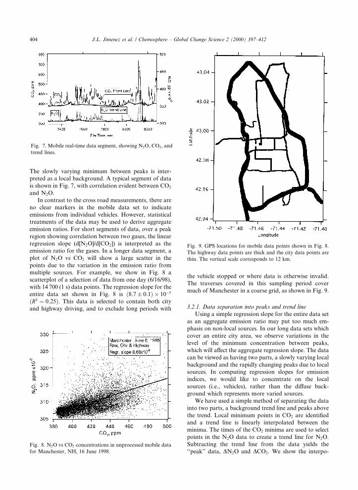
The slowly varying minimum between peaks is inter-
preted as a local background. A typical segment of data
is shown in Fig. 7, with correlation evident between CO2
and N2O.
In contrast to the cross road measurements, there are
no clear markers in the mobile data set to indicate
emissions from individual vehicles. However, statistical
treatments of the data may be used to derive aggregate
emission ratios. For short segments of data, over a peak
region showing correlation between two gases, the linear
regression slope (d[N2O]/d[CO2]) is interpreted as the
emission ratio for the gases. In a longer data segment, a
plot of N2O vs CO2 will show a large scatter in the
points due to the variation in the emission ratio from
multiple sources. For example, we show in Fig. 8 a
scatterplot of a selection of data from one day (6/16/98),
with 14 700 (1 s) data points. The regression slope for the
entire data set shown in Fig. 8 is �8:7� 0:1� � 10ÿ5
�R2 � 0:25�. This data is selected to contain both city
and highway driving, and to exclude long periods with
the vehicle stopped or where data is otherwise invalid.
The traverses covered in this sampling period cover
much of Manchester in a coarse grid, as shown in Fig. 9.
3.2.1. Data separation into peaks and trend line
Using a simple regression slope for the entire data set
as an aggregate emission ratio may put too much em-
phasis on non-local sources. In our long data sets which
cover an entire city area, we observe variations in the
level of the minimum concentration between peaks,
which will a�ect the aggregate regression slope. The data
can be viewed as having two parts, a slowly varying local
background and the rapidly changing peaks due to local
sources. In computing regression slopes for emission
indices, we would like to concentrate on the local
sources (i.e., vehicles), rather than the di�use back-
ground which represents more varied sources.
We have used a simple method of separating the data
into two parts, a background trend line and peaks above
the trend. Local minimum points in CO2 are identi®ed
and a trend line is linearly interpolated between the
minima. The times of the CO2 minima are used to select
points in the N2O data to create a trend line for N2O.
Subtracting the trend line from the data yields the
``peak'' data, DN2O and DCO2. We show the interpo-
Fig. 7. Mobile real-time data segment, showing N2O, CO2, and
trend lines.
Fig. 8. N2O vs CO2 concentrations in unprocessed mobile data
for Manchester, NH, 16 June 1998.
Fig. 9. GPS locations for mobile data points shown in Fig. 8.
The highway data points are thick and the city data points are
thin. The vertical scale corresponds to 12 km.
404 J.L. Jimenez et al. / Chemosphere ± Global Change Science 2 (2000) 397±412

lated trend lines in our typical sample of data in Fig. 7.
A similar procedure has been used in a recent aircraft
study of emissions in Athens (Klemm and Ziomas,
1997). Drawing a trend line is straightforward for iso-
lated peaks that clearly rise from and return to a ¯at
background. It is less straightforward when there are
multiple peaks close together or when there is a ¯uctu-
ating concentration without a clear background. There
is some subjectivity in the selection of minimum points,
but the method should give a more accurate represen-
tation of the contributions of local sources than the raw
data set. The raw data for CO2 (average 419:7� 30:5ppm), is separated into a trend line part (average
403:1� 15:8 ppm) and a peak part (average 16:6� 24:7ppm), where the errors given represent the standard
deviation of the data sample. Similarly, the raw data for
N2O (average 309:9� 5:3 ppm) is separated into a trend
line part (average 307:8� 1:7 ppm) and a peak part
(average 2:1� 4:5 ppm). Thus, the trend line data is the
majority of the total gas concentration, but with less
statistical variability. The peak fractions are small, with
standard deviations greater than their means.
A scatterplot (Fig. 10) of DN2O vs DCO2 for the peak
data shows a wide spread of points and a cluster of
points near DN2O � 0; DCO2 � 0, but without the
dense band of points due to varying background seen in
Fig. 8. A linear regression ®t to the peak data gives a
somewhat higher slope than the raw data set, for an
emission ratio from this data aggregation of
�10:9� 0:1� � 10ÿ5 �R2 � 0:36). A linear regression for
the slowly varying trend line data shows a smaller slope,
for a background emission ratio of �4:41� 0:09� � 10ÿ5
�R2 � 0:15�.
If each pair of DN2O and DCO2 data points is rati-
oed, we generate a set of �104 emission ratio samples,
which then can be used to form distributions as well as
averages. Selections and conditions can be applied easily
to the set of pointwise ratios, in order to ®nd the best
data subset for emission index determination and to test
dependencies. The ®rst selection is to consider the
highway plus city roadway data set used in the scatter-
plots above (Figs. 8 and 10). Next, we select data with
DCO2 greater than a minimum level (above the sub-
tracted background). The minimum DCO2 elevation
selection excludes data close to the background, which
can be negative for either DCO2 or DN2O. Thus, we
reduce contamination of the ratio distribution with
negative or spuriously large values. We empirically set
the DCO2 cuto� to be 15 ppm (close to the average for
the whole ``peaks'' set), which eliminates 52% of the data
points, with 5538 remaining. The cuto� value is selected
by observing the e�ect of increasing cuto� on the ratio
distribution. There is a large change going from zero
cuto� to 10 ppm, but quite small changes from 10 to
20 ppm.
The selected normalized distribution of emission ra-
tios (determined on a point by point basis) from mobile
measurements is shown in Fig. 11. From this distribu-
tion, we derive our reported average emission ratio of
�12:8� 0:3� � 10ÿ5. The uncertainty in the mean is pri-
marily systematic, estimated from the variation in the
mean with changes in DCO2 cuto�. The distribution has
a similar shape as that observed in cross road mea-
surements. The distribution is skewed, with a peak at
low values and an exponentially decreasing tail. The
width of the distribution in terms of standard deviation
is �10� 10ÿ5.
Fig. 10. N2O vs CO2 concentrations for the ``peak'' segment of
the mobile data.
Fig. 11. Histogram of pointwise ratios for mobile peak data,
DN2O/DCO2, city and highway, DCO2 > 15 ppm.
J.L. Jimenez et al. / Chemosphere ± Global Change Science 2 (2000) 397±412 405

The data can be segregated to test the e�ect of po-
tential controlling variables. For example, if we divide
the data contained in Fig. 11 into highway vs city roads,
then we observe a di�erence in the emission ratio:
�10:9� 0:3� � 10ÿ5 for the highway vs �15:6� 0:3��10ÿ5 for the city roads. A separation of the data into
two groups with speed less than or greater than 16 m/s
(36 mph) shows a similar di�erence in the emission ratio,
re¯ecting the tra�c speed di�erence between city and
highway roads. Thus, the grouping of data by city-
highway or slow-fast represents the same classi®cation,
with a robust di�erence in the N2O emission ratios. This
di�erence is probably due to the smaller fraction of ve-
hicles in cold start on the highway, and also to the higher
catalyst temperatures at higher speeds, both of which
result in lower N2O emissions (Rabl et al., 1997; Odaka
et al., 1998). We tested other grouping methods, (posi-
tive vs negative acceleration, positive vs negative vertical
climb rate) and found much smaller di�erences in
emission ratios.
We have considered the question of possible depen-
dence of our emission index distribution on the method
of grouping data. The data might be grouped into larger
blocks, each of which contains one (or a few) peaks. The
set of minimum points used to identify the local back-
ground provides a convenient way to segment the data
into relatively small blocks. Some of these segments are
individual peaks, and some contain clusters of peaks.
We calculated regression slopes (d[N2O]/d[CO2]) for
each of the � 250 peak segments contained in the scat-
terplot (Fig. 10). The peaks have an average width in
time of 28� 32 s, covering an average distance of
460� 680 m, so we expect that many vehicles contribute
to each peak. The set of slopes forms a distribution of
emission indices, shown in Fig. 12. Also shown in Fig. 12
is the distribution based on point by point analysis.
Similar results are obtained for the two analysis
methods, aggregation by peak-segment and point by
point ratio analysis, both in terms of average and stan-
dard deviation, and in the shape of the distribution.
Point by point analysis o�ers the advantage of the ease
of application of cuts based on instantaneous variables,
such as speed or location. The point by point ratio dis-
tribution can be interpreted as a distribution of the
probability of encountering a given emission ratio from
local sources in the urban area. Each sample point may
contain contributions from more than one vehicle, ef-
fectively averaging the measurement to some degree.
Averaging will tend to decrease the extremes of the
distribution, at both high and low values.
4. Discussion
We have presented vehicular N2O emissions data
which was collected with two di�erent TILDAS instru-
ments utilized in two di�erent experimental con®gura-
tions (cross road remote sensing and mobile extractive
sampling) and in two di�erent settings (southern Cali-
fornia and Manchester, New Hampshire). We obtain
comparable values for the ``raw'' average emissions
ratios from these two di�erent measurements, i.e.,
without extrapolating to a consistent tra�c mix by
taking into account the e�ects in the mobile data of
vehicles without catalytic converters or heavy duty
trucks. The emission ratio determined by cross road
remote sensing (corresponding to cars with catalytic
converters) is �8:8� 2:8� � 10ÿ5 and the mobile extrac-
tive sampling value (for all data points, corresponding to
mixed tra�c) is �12:8� 0:3� � 10ÿ5. The mobile data
shows a systematically higher emission ratio for the city
roads (�15:6� 0:3� � 10ÿ5) than for the highway
(�10:9� 0:3� � 10ÿ5).
The distributions of the two data sets (cross road
and mobile) are similar, especially the exponential tails
at high emission values, as seen in Fig. 13. The distri-
butions are more distinct close to zero. The cross road
distribution has a more substantial population with
``negative'' emissions, due to the sensitivity limit (and
hence random error) of 8 ppmv of the exhaust
(6� 10ÿ5 emission ratio). The mobile measurements
also have a random error, which depends in part on the
e�ect of the peak-trend separation procedure. The basic
instrumental noise of the mobile measurements is
�1 ppb for N2O and �1 ppm for CO2. The presence of
negative emission ratios in the mobile measurements
Fig. 12. Histogram of regression slopes, N2O vs CO2, for 251
segments of mobile data. The histogram of pointwise ratios is
superimposed, dotted line.
406 J.L. Jimenez et al. / Chemosphere ± Global Change Science 2 (2000) 397±412

indicates a random error for each ratio point of
�3� 10ÿ5.
More detailed comparison of our cross road and
mobile measurements will involve extrapolations, due to
incomplete information and di�erences in the mix of
vehicles, operating conditions and other experimental
variables. In the cross road measurements, practically all
the vehicles were fully warmed up, the average speed was
13:6� 2:6 m=s; �99% of the vehicles (in the complete
data set) had catalytic converters, and there were no
heavy duty trucks. The cross road study was conducted
in California, where gasoline contained only 30 ppm of
sulfur, while the mobile measurement was conducted in
an area where gasoline contained sulfur levels near
300 ppm. Michaels (1998) found that lower sulfur con-
tent of gasoline resulted in lower N2O emissions, pos-
sibly another reason for the lower result in the cross
road study. In the mobile measurements, there may have
been vehicles in ``cold start'' conditions, especially in the
city. The mix of vehicles in Manchester was not char-
acterized, but there were certainly large diesel trucks
without catalytic converters in the sample. The mobile
measurement van had an average speed of 16:5� 9:7 m/
s, moving with tra�c in the city and somewhat slower
than tra�c on the highway. The range of operating
conditions, locations and the variety of vehicles was
greater in the mobile measurements. For completeness
we note two other di�erences, the more stringent emis-
sions standards for California as compared to the rest of
the country; and the 1.5 year time di�erence between the
studies.
4.1. Comparison with previous work
In order to compare our results to previous work, we
must account for the wide variety of the literature on
nitrous oxide emissions, in terms of the types of studies,
measured quantities, number and type of measured ve-
hicles, and units to express emissions. Previous studies of
nitrous oxide emissions from motor vehicles have been
of two main types, dynamometer studies and tunnel
studies. The dynamometer studies are extensive exam-
inations of a small number of vehicles, with the advan-
tages of known vehicle characteristics and driving
conditions, but also with the disadvantage that it is
di�cult to study enough vehicles to characterize ¯eet
emissions. This is especially true if the emissions distri-
bution is skewed, as we have shown to be the case for
nitrous oxide. The tunnel studies sample the emissions
from thousands of vehicles, which allows them to ac-
quire statistically robust averages. The tunnel studies
also naturally report emission indices (molar ratios of
N2O to CO2), which are the same quantities that we
measure. We therefore focus on comparing our results to
the tunnel studies, both in terms of emission indices for
mixed tra�c and for catalyst equipped automobiles.
The comparison of our work to tunnel studies is
complicated by the e�ects of sampling mixed exhaust
from numerous vehicles. Unlike our cross road mea-
surements of individual vehicles, our mobile sampling
and previous tunnel studies cannot separate the emis-
sions of catalyst equipped automobiles from those of
automobiles and heavy duty vehicles which lack cata-
lysts. The e�ect of heavy duty trucks in mixed tra�c is
especially important, since they are strong sources of
CO2 and their N2O emissions are uncertain. They may
constitute �10% of the tra�c, but emit 25±40% of the
total exhaust due to their lower fuel economy. To derive
emission factors for catalyst equipped vehicles from
previous tunnel studies and from our mobile van mea-
surements, one must make assumptions about the N2O
emissions of automobiles without catalysts and of heavy
duty vehicles and further assumptions about the relative
fuel economy of these vehicles.
In Table 2, we compare our work to four earlier
tunnel studies (Berges et al., 1993, counted as two
studies, Sj�odin et al., 1998 and Becker et al., 2000). We
show the measured emission indices for mixed tra�c and
then derive the emission indices for catalyst equipped
vehicles, based on the reported tra�c mixtures and two
distinct sets of assumptions regarding the vehicles
without catalysts. We apply a uniform set of assump-
tions to di�erent studies in order to clarify the sensitivity
of the derived (catalyst equipped vehicle) emission in-
dices to those assumptions, and to see if the variation
Fig. 13. Normalized histograms of emission ratios from cross
road (thick line) and mobile measurements (thin line). Cross
road bin widths are 0:035� 103 and the mobile bin widths are
0:02� 103.
J.L. Jimenez et al. / Chemosphere ± Global Change Science 2 (2000) 397±412 407

between results is due in part to di�erent assumptions.
In analysis Case I, we assume that vehicles without
catalysts emit zero nitrous oxide and that the fuel
economy of heavy duty vehicles is four times smaller
than that of light duty vehicles. Case I is similar to the
analysis performed by Berges et al. (1993). In Case II, we
make the more realistic assumptions that light duty ve-
hicles without catalysts emit nitrous oxide with an
emission index of 4:5� 10ÿ5 (Jimenez, 1999), and that
heavy duty vehicles also emit nitrous oxide with an
emission index of 2:5� 10ÿ5 (Dietzmann et al., 1980),
and that the fuel economy of the heavy duty trucks is
four times smaller than that of light duty vehicles. Nei-
ther case is likely to be exactly correct, nor would any
one set of assumptions be perfectly appropriate for all
®ve studies. Still, the two cases show a range of rea-
sonable interpretations based on our current under-
standing.
The analysis presented in Table 2 produces a derived
emission factor for catalyst equipped vehicles from our
mobile measurements which is approximately twice as
large as our cross road result. Our cross road result is the
same in all three columns of the table since we know that
that value corresponds to catalyst equipped vehicles. In
a study of two tunnels with mixed tra�c, Berges et al.
(1993) derived an emission index for catalyst equipped
vehicles of �38� 22� � 10ÿ5, based on smaller measured
molar ratios (6� 10ÿ5 in Germany in 1992 and
14� 10ÿ5 in Sweden in 1992), by assuming that vehicles
lacking catalysts produced zero nitrous oxide. When we
apply our Case II analysis and assumptions to their data
we arrive at lower emission indices, but which are still
more than twice our cross road value. The more recent
studies of Sj�odin et al. (1998) and Becker et al. (2000),
report smaller emission indices of 4:6� 10ÿ5 and
4:1� 10ÿ5, and our analysis yields extrapolated emission
indices closer to our cross road results. The extrapolated
emission indices are slightly more variable than the raw
values, so uniform assumptions about tra�c mix do not
reduce the variation in the results of these studies. We
have not been able to reconcile the results of the existing
studies with other assumptions about the tra�c mixes. It
appears that either nitrous oxide emissions of catalyst
equipped vehicles are systematically di�erent in these
studies or there are signi®cant errors in some of the
measurements.
We also compare our results to dynamometer studies,
since most of the published studies of N2O emissions
from motor vehicles are of that type. In Fig. 14 we plot
the reported results from several dynamometer studies
as well as those of the studies with large vehicle samples
discussed above, using the common basis for compari-
son of N2O emission rate in mg/mile for vehicles with
aged TWCs. For the dynamometer studies in Fig. 14 we
only include data for passenger cars equipped with
TWCs, and only vehicles that have accumulated at least
a few thousand miles, if the relevant papers provide
mileage information. We have not included the study of
Ballantyne et al. (1994) since their emission rates are
overestimated due to unsubtracted ambient N2O levels
(Barton and Simpton, 1994). For the tunnel and mobile
studies we show our best estimates for aged three-way
catalyst vehicles (Case II in Table 2) and assume a fuel
economy of 25 miles/gallon (10.6 km/l). In our cross
road study, the emission rate is calculated using average
fuel consumption rates for each model year of the in-
dividual vehicles observed (Heavenrich and Hellman,
1996).
The dynamometer study results plotted in Fig. 14
show higher N2O emission rates, with an average
(weighted by the number of vehicles in each study) of
78� 50 mg/mile. The average of the four tunnel studies
and our two values (cross road and mobile) is 49� 28
mg/mile. The higher average of the dynamometer stud-
ies could be because they include cold starts in the
driving cycles. The larger apparent variability of the
Table 2
Comparison of nitrous oxide emission indices from four tunnel studies with this worka
Study Location Date Measured EIb Derived EI
Case Ic
Derived EI
Case IId
Berges (1993) Sweden 1992 14 28.0 23.5
Berges (1993) Germany 1992 6 43.9 20.9
Sj�odin (1998) Sweden 1994 4.6 13.3 6.6
Becker (2000) Germany 1997 4.1 7.6 4.9
This wsrk: Cross road California 1996 8.8 8.8 8.8
This work: Mobile New Hampshire 1998 12.8 18.5 17.4
a The earlier tunnel study by Sj�odin et al. (1995) is not included in the table because a N2O/CO2 ratio was not reported.b All emission indices (EI) are multiplied by 105, i.e., 14 corresponds to molar ratio N2O=CO2 � 14� 10ÿ5.c Case I emission factors are derived assuming that vehicles without catalysts emit zero nitrous oxide and that the fuel economy of
heavy duty trucks is four times smaller than that of light duty vehicles. The tra�c mixes are taken from the relevant publications. For
our mobile van measurements we assume that the tra�c mix is 90% catalyst equipped light duty vehicles and 10% heavy duty vehicles.d Case II emission factors use the same assumptions as Case I except that light duty vehicles without catalysts are assigned an emission
index of 4:5� 10ÿ5 (Jimenez, 1999) and heavy duty vehicles are assigned an emission index of 2:5� 10ÿ5 (Dietzmann, 1980).
408 J.L. Jimenez et al. / Chemosphere ± Global Change Science 2 (2000) 397±412

dynamometer studies in Fig. 14 can be explained by
small sample sizes. For example, the ®ve studies that
only involved one vehicle resulted in most of the extreme
(both high and low) emission rates. The study by De
Soete (1989) reports a value based on measurements of a
single vehicle which is high when compared to the
studies summarized in Fig. 14 (cf. Joumard et al., 1996;
Knapp, 1990; Koike and Odaka, 1996; Smith and Carey,
1982; Warner-Selph and Harvey, 1990). That high value
was essentially adopted as the 1996 IPCC emission
factor for the US (IPCC, 1996; Michaels, 1998). The
most recent estimates from the US EPA (Michaels,
1998) for cars with ``early'' and ``advanced'' TWCs are
also shown. Cars with ``advanced'' TWCs were phased
in during 1992±93 in California and 1994±95 in the rest
of the U.S. The estimates for both types are within the
range spanned by the tunnel, cross road, and mobile
studies.
4.2. Implications for the global N2O budget
An important question is how useful our results can
be in predicting the total N2O emissions of vehicles in
the US and throughout the world. Often the ®rst step in
such an estimation is to separately consider the contri-
butions of vehicles with and without catalysts, and to
attribute the majority of emissions to vehicles with cat-
alysts. We have generated detailed information on a
large number of catalyst equipped vehicles in our cross
road study. A model to extrapolate emissions to na-
tional or global ¯eets would take into account the nu-
merous variables which are known to a�ect N2O
emissions, including vehicle type, power demand, cata-
lyst type and aging, and the sulfur content of the fuel.
Also, the emission rate for individual vehicles varies
through driving cycles as the catalyst temperature
changes, with the highest emissions occurring during the
``cold start'' phase (Braddock, 1981; Jobson, et al., 1994;
Laurikko and Aakko, 1995). Some of these catalyst re-
lated e�ects could alter ¯eet emission estimates by a
factor of two (Jimenez, 1999). Fleet emissions also
will have an uncertain contribution from non-catalyst
vehicles.
Short of making a detailed model based estimate of
¯eet emission of N2O, our data may be useful in setting
bounds on ¯eet emissions. Berges et al. (1993) used
a simple analysis of ¯eet emissions to predict that
automobiles would be a large and growing source of
Fig. 14. Comparison of N2O emission rates for passenger cars with TWC for several dynamometer studies, tunnel studies, the work
reported here, and two o�cial estimates. The numbers above the bars indicate the number of vehicles in the studies. The bars with stars
represent the average of the dynamometer studies, weighted by the number of vehicles, and the average of the tunnel studies and our
two values, equally weighted.
J.L. Jimenez et al. / Chemosphere ± Global Change Science 2 (2000) 397±412 409

atmospheric N2O. They calculated that if the entire ¯eet
of existing automobiles were equipped with present day
catalysts, and using their emission index of
�38� 22� � 10ÿ5, then the nitrous oxide emissions from
cars could reach 6±32% of the atmospheric growth rate
of nitrous oxide. In this work we ®nd much lower
emission indices for catalyst equipped vehicles, of only
9� 10ÿ5 and 17� 10ÿ5, from cross road and mobile
measurements. An analysis similar to Berges et al. based
on our two values implies that the above scenario would
produce a less alarming result, with N2O emission rates
reaching between 4% and 7% of the atmospheric growth
rate, using our cross road and mobile emission rates,
respectively.
The best way to answer the question of estimating
¯eet emissions may be to perform many more mea-
surements of vehicles at di�erent locations and under
varying conditions. For catalyst equipped vehicles, more
work is required to better quantify the e�ects of vehicle
type, driving cycle, catalyst type and age, and fuel
chemistry, especially as they apply to real world vehicles
and driving patterns. It also is important to better
quantify the emissions of vehicles without catalytic
converters such as heavy duty diesel trucks.
5. Summary
We have used two di�erent TILDAS based tech-
niques to measure the N2O/CO2 emission ratios of on-
road motor vehicles. Cross road, open path laser mea-
surements of emissions from 1361 vehicles in California
yielded an average emission ratio (N2O/CO2) of
�8:8� 2:8� � 10ÿ5 for catalyst equipped vehicles. A van-
mounted TILDAS sampling system making on-road
N2O measurements in Manchester, New Hampshire
yielded an average ratio of �12:8� 0:3� � 10ÿ5 for mixed
tra�c, including heavy duty vehicles. The mobile data
shows a systematically higher emission ratio for the city
roads (�15:6� 0:3� � 10ÿ5) than for the highway
(�10:9� 0:3� � 10ÿ5). Average N2O/CO2 emission ratios
for each TILDAS technique are comparable, and their
distributions are similar, even though the measurement
circumstances were quite di�erent. The average emission
rates obtained in both our cross road and mobile mea-
surements are within the range of values reported in
recent tunnel studies. Our measured distributions are
skewed, with a small number of high N2O emitters and a
majority of low emitters, similar to the distributions of
CO, NO and HCs seen in previous studies.
The cross road measurements, when combined with
individual vehicle identi®cation, allow detailed analysis
of the dependence of N2O emissions on a variety of
factors, including vehicle type and model year, vehicle
speci®c power, and the emissions of other gases. LTDs
have higher emissions than passenger cars, which is only
partially explained by their lower fuel economy. We
observed no signi®cant dependence on vehicle age nor
strong correlation between high N2O emitters and NO,
CO, or HC high emitters. We also observed a general
trend of increasing N2O emission as the vehicle speci®c
power increases.
The mobile measurements provide data on the
emissions of a large number of vehicles across an urban
area in real world driving situations. Average emission
ratios and probability distributions can be derived for
di�erent conditions. The clearest distinction we see is
between emission ratios for city roads (at low speed) and
highways (at high speed), with the city emission ratio
43% higher than on the highway. Direct measurement of
many vehicles across a wide area may help to reduce the
uncertainties of model-based projections of vehicle ¯eet
emissions.
Berges et al. (1993) calculated that if the entire ¯eet of
existing automobiles were equipped with present day
catalysts the nitrous oxide emissions from cars could
reach 6±32% of the atmospheric growth rate of this
species. A similar analysis based on our measurements
implies that the above scenario would produce a less
alarming result, with N2O emission rates reaching be-
tween 4% and 7% of the atmospheric growth rate, using
our cross road and mobile emission rates, respectively.
More work is needed to understand the large di�erences
between the existing studies.
Acknowledgements
The cross road studies reported here were funded by
the US Environmental Protection Agency and Califor-
nia's South Coast Air Quality Management District.
The mobile measurements were sponsored by the EOS/
IDS program of the O�ce of Earth Sciences at the
National Aeronautics and Space Administration. The
assistance of Stephen E. Schmidt of Arthur D. Little,
Inc. in designing and executing the cross road mea-
surements, and for providing the license plate recording
system is gratefully acknowledged. We thank Michael
Gray, Jay Peterson and Michael Terorde of the Hughes
Santa Barbara Research Center, and Nelson Sorbo of
Hughes Environmental Services for their assistance
during the cross road campaign. We are grateful for the
assistance of the O�ce of the Mayor and the Depart-
ment of Public Works in Manchester, New Hampshire,
as well the New Hampshire Technical College.
References
Ballantyne, V.F., Howes, P., Stephanson, L., 1994. Nitrous
oxide emissions from light duty vehicles. Society of Auto-
motive Engineers Paper 940304.
410 J.L. Jimenez et al. / Chemosphere ± Global Change Science 2 (2000) 397±412

Barton, P., Simpson, J., 1994. The e�ects of aged catalysts and
cold ambient temperatures on nitrous oxide emissions.
MSED Report #94±21, Technology Development Direc-
torate, Environment Canada: Ottawa, Canada.
Becker, K.H., L�orzer, J.C., Kurtenbach, R., Wiesen, P., Jensen,
T., Wallington, T.J., 1999. Nitrous oxide (N2O) emissions
from vehicles. Environ. Sci. Technol. 33, 4134±4139.
Becker, K.H., L�orzer, J.C., Kurtenbach, R., Wiesen, P., Jensen,
T., Wallington, T.J., 2000. Contribution of vehicle exhaust
to the global N2O budget. Chemosphere ± Global Change
Science 2 (3±4) 387±395.
Berges, M.G.M., Hofmann, R.M., Schar�e, D., Crutzen, P.J.,
1993. Nitrous oxide emissions from motor vehicles in
tunnels and their global extrapolation. J. Geophys. Res.
98 (18), 527±531.
Bishop, G.A., Starkey, J.R., Ihlenfeldt, A., Williams, W.J.,
Stedman, D.H., 1989. IR long path photometry: a remote
sensing tool for automobile emissions. Anal. Chem. 61,
671A±677A.
Braddock, J.N., 1981. Impact of low ambient temperature on 3-
way catalyst car emissions. Society of Automotive Engineers
Paper 810280.
Cant, N.W., Angove, D.E., Chambers, D.C., 1998. Nitrous
oxide formation during the reaction of simulated exhaust
streams over rhodium, platinum and palladium catalysts.
Appl. Catalysis B 17, 63±73.
Cicerone, R.J., 1989. Analysis of sources and sinks of atmo-
spheric nitrous oxide (N2O). J. Geophys. Res. 94, 18265±
18271.
Dasch, J.M., 1992. Nitrous oxide emissions from vehicles. J. Air
Waste Manage. Assoc. 42, 63±67.
De Soete, G., 1989. Updated evaluation of nitrous oxide
emissions from industrial fossil fuel combustion. Draft ®nal
report for the European Atomic Energy Community,
Institut Francais du Petrole, Rueil-Malmaison, France.
Dietzman, H.E., Parness, M.A., Bradow, R.L.,1980. Emissions
of trucks by chassis version of 1983 transient procedure.
Society of Automotive Engineers Paper 801371.
Hargreaves, K.J., Weinhold, F.G., Klemedtsson, L., Arah,
J.R.M., Beverland, I.J., Fowler, D., Galle, B., Gri�th,
D.W.T., Skiba, U., Smith, K.A., Welling, M., Harris, G.W.,
1996. Measurement of nitrous oxide emissions from agri-
cultural land using micrometeorological methods. Atmos.
Environ. 30, 1563±1571.
Heavenrich, R.M.K.H., Hellman 1996. Light-Duty Automotive
Technology and Fuel Economy Trends Through 1996. US
Environmental Protection Agency, Ann Arbor, Michigan.
IPCC, 1996. Climate Change 1995: The Science of Climate
Change. Contribution of Working Group I to the Second
Assessment Report of the Intergovernmental Panel on
Climate Change. Cambridge University Press, Cambridge,
U.K.
Jack, M.D., et al., 1995. Remote and on-board instrumentation
for automotive emissions monitoring. Society of Automo-
tive Engineers Paper 951943.
Jimenez, J.L., Nelson, D.D., Zahniser, M.S., McManus, J.B.,
Kolb, C.E., Koplow, M.D., Schmidt, S.E., 1997. Remote
sensing measurements of on-road vehicle nitric oxide
emissions and of an important greenhouse gas: nitrous
oxide. In: Seventh CRC On-Road Vehicle Emissions
Workshop, San Diego, CA.
Jimenez, J.L., Koplow, M.D., Nelson, D.D., Zahniser, M.S.,
Smith, S.E., 1999. Characterization of on-road vehicle NO
emissions by a TILDAS remote sensor. J. Air Waste
Manage. Assoc. 49, 463±470.
Jimenez, J.L., 1999. Understanding and quantifying motor
vehicle emissions with vehicle speci®c power and TILDAS
remote sensing. Ph.D. Thesis, Massachusetts Institute of
Technology, Cambridge, MA.
Jobson, E., Smedler, G., Maimberg, P., Bernier, H., Hjortsberg,
O., 1994. Nitrous oxide formation over three-way catalyst.
Society of Automotive Engineers Paper 940926.
Joumard, R., Vidon, R., Paturel, L., DeSoete, G., 1996.
Changes in pollutant emissions from passenger cars under
cold start conditions. Society of Automotive Engineers
Paper 961133.
Khalil, M.A.K., Rasmussen, R.A., 1992. The global sources of
nitrous oxide. J. Geophys. Res. 97, 14651±14660.
Klemm, O., Ziomas, I.C., 1997. Urban emissions measured
with aircraft. J. Air Waste Manage. Assoc. 48, 16±25.
Knapp, K., 1990. Continuous FTIR measurements of mobile
source emissions. European Workshop on the emissions of
N2O, Lisbon, Portugal.
Koike, N., Odaka, M., 1996. Methane and nitrous oxide
emissions characteristics from automobiles. Society of
Automotive Engineers Paper 960061.
Kroeze, C., Mozier, A., Bouwman, L., 1999. Closing the global
N2O budget: A retrospective analysis 1500±1994. Global
Biogeochem. Cycles 13, 1±8.
Laurikko, J., Aakko, P., 1995. The e�ect of ambient temper-
ature on the emissions of some nitrogen compounds: A
comparative study on low-, medium- and high mileage
three-way catalyst vehicles. Society of Automotive Engi-
neers Paper 950933.
Michaels, H. 1998. Emissions of nitrous oxide from highway
mobile sources: comments on the draft inventory of US
greenhouse emissions and sinks 1990±96, US Environmental
Protection Agency, Ann Arbor, Michigan.
NRC, 1993. Understanding and Predicting Atmospheric Chem-
ical Change. National Research Council, National Academy
Press, Washington, DC.
Nelson, D.D., Zahniser, M.S., McManus, J.B., Kolb, C.E.,
Jimenez, J.L., 1998. A tunable diode laser system for the
remote sensing of on-road vehicle emissions. Appl. Phys. B
67, 433±441.
Nelson, D.D., McManus, J.B., Zahniser, M., Kolb, C.E., 1999.
Laser system for cross road measurement of motor vehicle
exhaust gases. US Patent No. 5,877,862.
Odaka, M., Koike, N., Suzuki, H., 1998. Deterioration e�ect of
three-way catalyst on nitrous oxide emission. Society of
Automotive Engineers Paper 980676.
Podolske, J., Lowenstein, M., 1993. Airborne tunable diode
laser spectrometer for trace-gas measurement in the lower
stratosphere. Appl. Opt. 32, 5324±5333.
Prigent, M., De Soete, G., Doziere, R., 1991. The e�ect of aging
on nitrous oxide (N2O) formation by automotive three-way
catalysts. In: A. Crucq, (Ed.), Catalysis and Automotive
Pollution Control. Elsevier, Amsterdam, The Netherlands.
Prigent, M., Castagna, F., Doziere, R., 1994. Status on nitrous
oxide emissions of three-way catalyst equipped vehicles. In:
Sixth International Workshop on Nitrous Oxide Emissions,
Turku, Finland.
J.L. Jimenez et al. / Chemosphere ± Global Change Science 2 (2000) 397±412 411

Rabl, H.-P., Gifhorn, A., Meyer-Pitro�, R., 1997. The forma-
tion of nitrous oxide (N2O) over three-way catalysts. In:
Fourth International Conference on Technologies and
Combustion for a Clean Environment, Lisbon, Portugal.
Rothman, L.S., Gamache, R.R., Tipping, R.H., Rinsland, C.P.,
Smith, M.A.H., Benner, D.C., Devi, M., Flaud, J.M.,
Camy-Peyret, C., Perrin, A., Goldman, A., Massie, A.,
Brown, L.R., Toth, R.A., 1992. The HITRAN Molecular
Database: Editions of 1991 and 1992. J. Quant. Spectrosc.
Radiat. Transf. 48, 467±507.
Shorter, J.H., McManus, J.B., Kolb, C.E., Allwine, E.J.,
O'Neill, S.M., Lamb, B.K., Scheuer, E., Crill, P.M., Talbot,
R.W., Ferreira, J. Jr., McRae, G.J., 1998. Recent measure-
ments of urban metabolism and trace gas respiration. In:
Proceedings of the 13th Conference on Biometeorology and
Aerobiology and the Second Urban Environ. Symp., Am.
Meteorol. Soc., Albuquerque, NM, pp. 49±52.
Sj�odin, A, Cooper, D.A., Andreasson, K., 1995. Estimates of
real-world N2O emissions from road vehicles by means of
measurements in a tra�c tunnel. J. Air Waste Manage.
Assoc. 45, 186±190.
Sj�odin, A., Persson, K., Andreasson, K.I., Arlander, B., Galle,
B., 1998. On-road emission factors derived from measure-
ments in a tra�c tunnel. Int. J. of Vehicle Design Vol. 20,
Nos. 1±4 (Special Issue).
Smith, L.R., Black, F.M., 1980. Characterization of exhaust
emissions from passenger cars equipped with three-way
catalyst control systems. Society of Automotive Engineers
Paper 800822.
Smith, L.R., Carey, P.M., 1982. Characterization of exhaust
emissions from high mileage catalyst equipped automobiles.
Society of Automotive Engineers Paper 820783.
Warner-Selph, M.A., Harvey, C.A., 1990. Assessment of
unregulated emissions from gasoline oxygenated blends.
Society of Automotive Engineers Paper 902131.
Webster, C.R., May, R.D., Trimble, C.A., Chave, R.G.,
Kendall, J., 1994. Aircraft (ER-2) laser infrared absorption
spectrometer (ALIAS) for in-situ atmospheric measure-
ments of HCl, N2O, CH4, NO2, and HNO3. Appl. Opt. 33,
454±472.
Zahniser, M.S., Nelson, D.D., McManus, J.B., Kebabian, P.K.,
1995. Measurement of trace gas ¯uxes using tunable diode
laser spectroscopy. Philos. Trans. R. Soc. Lond. 351, 371±
382.
Zhang, Y., Stedman, D.H., Bishop, G.A., Beaton, S.P.,
Guenther, P.L., McVey, I.F., 1996. Enhancement of remote
sensing for mobile source nitric oxide. J. Air Waste Manage.
Assoc. 46, 25±29.
Zhang, Y., Bishop, G.A., Stedman, 1994. Automobile emis-
sions are statistically c distributed. Environ. Sci. Technol.
28, 1370±1374.
Jose L. Jimenez recently received his doctorate in MechanicalEngineering from Massachusetts Institute of Technology (MIT)and is currently a research scientist at Aerodyne Research, Inc.(ARI) and a research a�liate at the MIT Chemical EngineeringDepartment; his doctoral thesis involved tunable infrared lasermeasurements and modeling of motor vehicle exhaust pollu-tants.
J. Barry McManus is a principal scientist at ARI, a physicistspecializing in the design and utilization of laser and otherelectro-optical measurement systems.
Joanne H. Shorter is a principal scientist at ARI and a physicalchemist who develops and uses laser sensors for environmentaltrace species measurements.
David D. Nelson is a principal scientist at ARI and a physicalchemist who utilizes laser spectroscopy for laboratory and ®eldstudies of atmospheric chemical kinetics and trace gas ¯uxes.
Mark S. Zahniser is a physical chemist and Director of ARI'sCenter for Atmospheric and Environmental Chemistry; hespecializes in spectroscopic and kinetic studies of atmospherictrace species.
M. Koplow is a mechanical engineer and the president of EM-DOT Corporation.
Gregory J. McRae is a professor of chemical engineering atMIT where local and regional air pollution issues are a majorfocus of his research group.
Charles E. Kolb is a physical and atmospheric chemist and ispresident of ARI.
412 J.L. Jimenez et al. / Chemosphere ± Global Change Science 2 (2000) 397±412