Cross sectional evaluation of the gut-microbiome metabolome axis in an Italian cohort of IBD patients

Maria Laura Santoru1, Cristina Piras1, Antonio Murgia2, Vanessa Palmas1, Tania Camboni1, Sonia Liggi1, Ivan Ibba3, Maria Antonia Lai4, Sandro Orrù3, Sylvain Blois1, Anna Lisa Loizedda5, Julian Leether Griffin6, Paolo Usai3, Pierluigi Caboni2, ^Luigi Atzori1, *Aldo Manzin1 1Department of Biomedical Sciences, University of Cagliari 2Department of Life and Environmental Sciences, University of Cagliari 3Department of Medical Sciences and Public Health, University of Cagliari and 4Gastroenterology Unit, University Hospital of Cagliari 5Consiglio Nazionale delle Ricerche (C.N.R.), Istituto di Ricerca Genetica e Biomedica ( I.R.G.B.), Monserrato, Cagliari, Italy 6Department of Biochemistry, University of Cambridge, Cambridge, UK

*Corresponding Author: Prof. Aldo Manzin: aldomanzin@medicina.unica.it +39-70-675 4067

AL^ and MA* contributed equally to this work.

METHODS

Gut microbiota

DNA extraction and quantification: 100-200 mg of fecal sample was mixed with 1.4-2.8 mL ASL buffer in

a 2 mL tube and vortexed until the sample was thoroughly homogenized. Lysis was carried out at a

temperature of 95°C for 5-10 minutes. Finally, DNA was extracted according to the instruction of the

QIAamp DNA stool MiniKit and eluted in 200 µL elution buffer provided in the kit. DNA concentration and

purity were measured using a NanoDrop ND-1000 spectrophotometer (Thermo Fisher Scientific), and

samples were stored at −80°C until further processing.

Real-time quantitative PCR. Primers: forward 5’-CCTACGGGNGGCWGCAG-3’; reverse 5’-

GACTACHVGGGTATCTAATCC-3’). Genomic DNA from the E. coli ATCC25922 reference isolate was

used to prepare the standard curve (1:10 dilutions from 70.5 to 0.0075 ng). The qPCR was performed using a

CFX96 Touch Real-Time System instrument (Bio-Rad) using the Bio-Rad CFX manager software, version

3.1 (Bio-Rad). Briefly, 20 µl PCR mixture contained 10 µl of SsoAdvanced Universal SYBR Green

Supermix (Bio-Rad), 8 pmol of each primer, and 5 µl of DNA elution were used for each reaction. qPCR

reactions consisted of an initial denaturation step of 5 min at 98°C, followed by 40 cycles of 15 s at 95°C,

and 20 s at 59°C. The specificity of each PCR was determined by the melting curve analysis where by the

temperature from 65°C to 95°C was increased with 0.5°C increments.

Library preparation and sequencing. For amplification reactions, fusion degenerate primer 16SF (5’-

TCGTCGGCAGCGTCAGATGTGTATAAGAGACAGCCTACGGGNGGCWGCAG-3’) and 16SR (5’-

GTCTCGTGGGCTCGGAGATGTGTATAAGAGACAGGACTACHVGGGTATCTAATCC-3’) were used,

with ligated overhang Illumina adapter consensus sequences as indicated above in the underlinedregion.

Each PCR reaction was carried out on an Applied Biosystem 9700 thermal cycler (Life Technologies) with 5

µL PCR buffer 10X, 0.5 µM each primer, 1.5 µL MgSO4 50 mM, 1 µL dNTP 10 mM each, 0.2 µL Platinum

Pfx DNA polymerase 5U/µL (Life Technologies), 12.5 ng total DNA template, and nuclease-free, DEPC-

treated water to a total volume of 50 µL. PCR reactions were performed as follows: after an initial

denaturing step at 95°C for 3 min, 35 cycles were carried out consisting of denaturation at 95°C for 30 sec,

annealing at 52°C per 30 sec, and extension at 72°C for 30 sec. After 35 cycles, the reaction was completed

with a final extension of 7 min at 72°C.

The 550 bp 16S amplicons were purified using 20 µL Agencourt AMPure XP magnetic beads (Beckman

Coulter) according to the manufacturer's instructions. For the multiplexing barcode procedure, the Illumina

Nextera XT Index kit with dual 8 bases indices were used. PCR reactions containing 25 µL of KAPA HiFi

HotStart Ready Mix 2x, 5 µL of i5 and i7 index (Illumina) each, 5 µL of purified amplicons, 5 µL Nextera

XT Index primer 2, and nuclease-free, DEPC-treated water to a final volume of 50 µL, were carried out on

an Applied Biosystem 9700 thermal cycler. PCR reactions consisted of one cycle of 95°C for 3 min,

followed by eight cycles of 95°C for 30 sec, 55°C for 30 sec, and 72°C for 30 sec, followed by a final

extension cycle of 72°C for 5 min. The barcoded amplicons were then purified using Agencourt AMPure XT

magnetic beads (Beckman Coulter, Inc.) following the instructions of the manufacturer. Afterwards, the

barcoded libraries were quantified using the Agilent High Sensitive DNA Kit (Agilent Technologies), and

normalized to ensure an equal representation of the samples. The quality and the size of the pooled libraries

were verified using Agilent DNA 1000 Analysis kit (Agilent Technologies) on the Agilent 2100 Bioanalyzer

system (Agilent Technologies), and finally sequenced on the MiSeq platform using MiSeq v3 Reagent Kit

(Illumina), with the adapter-ligated library PhiX v3 used as a control.

Metabolomics

Frozen feces (300 mg) were mixed with 800 µL of methanol containing succinic acid-2,2,3,3-d4 as an

internal standard (Sigma-Aldrich, St. Louis, MO, USA) and 200 µL of Milli-Q water and then vortexed.

After 30 min, samples were centrifuged at 14000 rpm for 10 min at 4°C. The supernatant was aliquoted as

following: GC-MS analysis (300 µL), LC-QTOF-MS analysis (50 µL) and NMR analysis (650 µL). For GC-

MS analysis 300 µL of each fecal extract were dried under vacuum with vacuum concentrator overnight and

were derivatised with 50 µL of methoxyamine dissolved in pyridine (10 mg/mL) (Sigma-Aldrich, St. Louis,

MO, USA). After 17 h 100 µL of N-Methyl-N-(trimethylsilyl)-trifluoroacetamide, (MSTFA, Sigma-Aldrich,

St. Louis, MO, USA) were added and left at room temperature for one hour. Successively, samples were re-

suspended in 400 µL of hexane (Sigma-Aldrich, St. Louis, MO, USA) and filtered with Acrodisc Syringe

Filters with 0.45 mm PTFE Membrane (SIGMA, St. Louis, MO, USA). For LC-MS QTOF analysis 50 µL of

fecal extract were transferred into an eppendorf tube and added to 316 µL methanol and 633 µL

dichloromethane. Samples were then centrifuged for 10 min at 12000 rpm. After centrifugation, the

supernatant was transferred to another eppendorf tube where 200 µL of water were added to induce phase

separation. All samples were then centrifuged at 8000 rpm for 10 min. The resulting organic phase was dried

under nitrogen, re-suspended in 300 µL methanol and then filtered with Acrodisc Syringe Filters with 0.45

mm PTFE Membrane (SIGMA, St. Louis, MO, USA) [1]. For NMR analysis, dried hydrophilic fecal

extracts were re-dissolved with 650 µL 100 mM KH2PO4/D2O buffer pH 7.2 (99,8%, Cambridge Isotope

Laboratories Inc, Andover, USA) and added with 50 µL of internal standard solution 5 mM (sodium 3-

trimethylsilyl-propionate-2,2,3,3,-d4, TSP, 98 atom % D, Sigma-Aldrich, Milan, Italy). An aliquot of 650 µL

was transferred to 5-mm NMR tubes.

GC-MS analysis. One microliter of derivatised sample was injected splitless into a 7890A gas

chromatograph coupled with a 5975C Network mass spectrometer (Agilent Technologies, Santa Clara, CA,

USA) equipped with a 30 m ×0.25 mm ID, fused silica capillary column, with a 0.25 µM TG-5MS stationary

phase (Thermo Fisher Scientific, Waltham, MA, USA). The injector and transfer line temperatures were at

250°C and 280°C, respectively. The gas flow rate through the column was 1 ml/min. For fecal samples

analysis the column initial temperature was kept at 60 °C for 3 min, then increased to 140°C at 7°C/min, held

at 140°C for 4 min, increased to 300°C at 5°C/min and kept for 1 min. Identification of metabolites was

performed using the standard NIST 08, and GMD mass spectra libraries and, when available, by comparison

with authentic standards.

1H-NMR spectroscopy analysis. 1H-NMR experiments were carried out using a Varian UNITY INOVA

500 spectrometer operating at 499.839 MHz for proton and equipped with a 5 mm double resonance probe

(Agilent Technologies, CA, USA). 1H-NMR spectra were acquired at 300K with a spectral width of 6000

Hz, a 90° pulse, an acquisition time of 2 s, a relaxation delay of 2 s, and 256 scans. The residual water signal

was suppressed by applying a presaturation technique with low power radiofrequency irradiation for 2 s. 1H

NMR spectra were imported in ACDlab Processor Academic Edition (Advanced Chemistry Development,

12.01, 2010) and pre-processed with line broadening of 0.1 Hz, zero-filled to 64K, and Fourier transformed.

Each spectrum was manually phased and baseline corrected. Chemical shifts were referred to the TSP single

resonance at 0.00 ppm. The 1H-NMR spectra were reduced into consecutive integrated spectral regions (bins)

of equal width (0.01 ppm) corresponding to the region 0.50–8.66 ppm. The spectral region between 4.74 and

4.94 ppm was excluded from the analysis to remove the effect of variations in the presaturation of the

residual water resonance. The integrated area within each bin was normalized to a constant sum of 100 for

each spectrum in order to minimize the effects of variable concentration among different samples. The final

data set was imported into the SIMCA-P+ program (Version 14.0, Umetrics, Sweden), mean-centered and

Pareto scaled column wise.

LC-QTOF-MS analysis. An Agilent 1200 series LC-QTOF-MS was used with an ESI source, operating in

the positive ion mode. The electrospray capillary, needle and shield potentials were set to 60 V, 5850 V, and

450 V respectively. Nitrogen at 48 mTorr and 375 °C was used as a drying gas. For the fecal extracts full-

scan spectra were obtained in the ranges of 100-1500 amu, scan time of 0.20 amu, scan width of 0.70 amu,

and detector at 1500 V. The organic layers were analysed by a Pheomenex Kinetek C18 column EVO (100A.

150x2.1 mm 5µ) (California, USA). The mobile phase consisted of: (A) 60% of 10 mM ammonium formate

and 40% of acetonitrile with 0.1% formic acid (v/v) and (B) a 10 mM ammonium formate solution

containing 90% of isopropanol, 10% of acetonitrile with 0.1% formic acid (v/v). The mobile phase was

pumped at a flow rate of 250 µL/min programmed as follows: initially at 68% of A for 1.30 min, then

subjected to a linear decrease from 68% to 3% of A in 30 min and was then brought back to the initial

conditions in 10 min. Putative recognition of all detected metabolites was performed using the Metlin and the

Lipid Maps databases, whereas the most statistically significant metabolites were subjected to further

identification with the means of targeted MS/MS analysis. Data were collected in the same m/z range of the

MS scan mode and collision energy was set at 30V. All the discriminant metabolites MS and MS/MS data

are reported (Supplementary table S4).

Data processing.

The R library XCMS [2, 3] was utilized for peak detection and retention time correction. Parameters utilized

for peak deconvolution for GC-MS matrices were manually optimized, whereas those used for LC-MS

matrices were optimised using the R library IPO [4]. Grouping of features into pseudospectra and annotation

of isotopes and adducts was performed using the standard parameters of the R library CAMERA [5]. The

resulting matrices were processed using an in-house python script to eliminate signals present in the blanks,

keep only the most abundant feature per molecule and modify all zeroes present in the matrix by inserting

half of the minimum value found for a feature. After manual correction of the filtered matrix to eliminate

internal standard and any possible remaining noise signal, median fold change normalization was performed

using an in-house python script in order to compensate for sample dilution biases [6].

Phyla Active vs. inactive CD

(p value)

Active vs. inactive UC

(p value)

Firmicutes 0,3099 0,8674

Bacteroidetes 0,9434 0,3410

Actinobacteria 0,1086 0,4597

Proteobacteria 0,6639 0,2723

Verrucomicrobia 0,2707 0,2584

Cyanobacteria 0,8820 0,6802

Fusobacteria 0,7204 0,3842

Table S1a Mann-Whitney test for Phyla abundance in active vs. inactive disease.

Phyla Colon vs Ileum CD (p value)

Firmicutes 0,2912

Bacteroidetes 0,9747

Actinobacteria 0,3510

Proteobacteria 0,3830

Verrucomicrobia 0,6256

Cyanobacteria 0,3816

Fusobacteria 0,0305

Table S1b Mann-Whitney test for Phyla abundance in colon vs. ileum localization of the disease.

Phyla CD therapy (p value) UC therapy (p value)

Firmicutes 0,0238 0,3431

Bacteroidetes 0,6208 0,2377

Actinobacteria 0,8172 0,0311

Proteobacteria 0,0950 0,0916

Verrucomicrobia 0,0217 0,1381

Cyanobacteria 0,8980 0,3429

Fusobacteria 0,3275 0,2222

Table S1c Kruskall-Wallis test for Phyla abundance and medications.

OPLS-DA models Permutation*

GC-MS

Groups Componentsa R2Xcumb R2Ycumc Q2cumd R2 intercept

Q2 intercept

Healthy vs IBD 1P+1O 0.112 0.663 0.439 0.333 -0.228

Healthy vs CD 1P+1O 0.144 0.778 0.519 0.478 -0.215

Healthy vs UC 1P+1O 0.119 0.734 0.504 0.408 -0.239

CD vs UC 1P+1O 0.105 0.494 0.036 0.419 -0.201

1H-NMR

Healthy vs IBD 1P+3O 0.495 0.754 0.626 0.188 -0.430

Healthy vs CD 1P+1O 0.314 0.730 0.645 0.231 -0.241

Healthy vs UC 1P+2O 0.458 0.805 0.688 0.181 -0.327

CD vs UC 1P+1O 0.202 0.440 0.140 0.257 -0.235

LC-MS/MS QTOF

Healthy vs IBD 1P+2O 0.429 0.504 0.393 0.270 -0.136

Healthy vs CD 1P+3O 0.429 0.786 0.433 0.587 -0.240

Healthy vs UC 1P+2O 0.451 0.620 0.494 0.345 -0.146

CD vs UC 1P+1O 0.369 0.311 0.0628 0.229 -0.056

Table S2 MVA parameters. a The number of Predictive and Orthogonal components used to create the statistical models. b,c R2X and R2Y indicated the cumulative explained fraction of the variation of the X block and Y block for the extracted components.

d Q2cum values indicated cumulative predicted fraction of the variation of the Y block for the extracted components. * R2 and Q2 intercept values are indicative of a valid model. The Permutation test was evaluated on the

corresponding partial least square discriminant analysis (PLS-DA) model.

PLS-DA models

Groups Componentsa R2Xcumb R2Ycumc Q2cumd

Active vs inactive CD 2 0.1 0.308 -0.0931

Active vs inactive UC 2 0.147 0.369 -0.21

Medications influence CD 3 0.126 0.406 -0.21

Medications influence UC 3 0.107 0.29 -0.169

Ileal vs colon CD 2 0.115 0.58 -0,19

Table S3 MVA parameters. a The number of components used to create the statistical models. b,c R2X and R2Y indicated the cumulative explained fraction of the variation of the X block and Y block for the extracted components. d Q2cum values indicated cumulative predicted fraction of the variation of the Y block for the extracted components.

Compound Parent ion m/z

Rt (min)

Adduct Product ion (m/z) Δppm

urobilin 617.3350 1.3 [M+Na] + 470 345

3

PC(16:0/3:1) 549.3461 1.4 neutral 184.0709 [Head group]+ 4 279.7294 1.7 urobilinogen 597.3670 2.2 [M+H]+ 472

347 3

508.4934 6.3 647.9453 11.0 515.3659 11.6 DG(16:0/18:2) 634.5398 12.3 [M+NH4]+ 313.2[RCOO+58]+ (FA16:0)

337.5[RCOO+58]+ (FA18:2) 1

PA (19:0/16:1) 688.5040 14.8 neutral 355 [RCOO+58] (FA19:0) 281 [RCO]+ (FA19:0)

0

PC (22.2/14:1) 783.5768 14.9 neutral 393 [RCOO+58]+ (FA22:2) 184.07 [Head group]+

0

371.3179 15.0 474.3812 15.5 465.3760 15.8 DG (18:0/22:2) 641.5974 16.4 [M+H2H2O]+ 267.0 [RCO]+

341.0 [RCOO+58]+ 14

PS (22:2/18:0) 844.6053 16.5 + H+ 341 [RCOO+58] (FA18:0) 319 [RCO]+ (FA22:2)

1

1238.874 20.8 Cer (18:1/22:0) 622.6167 22.7 +H+ 282 (FA18:1)

339 [RCOO+58] (FA18:1) 265 [RCO]+ (FA18:1)

0

1147.911 23.2 975.7294 23.2 1149.920 23.2 1076.719 23.5 465.3796 24.0 NAPE (18:1/16:1/18:0)

981.7768 25.9 neutral 265 [RCO]+ (FA18:1) 341 [RCOO+58]+ (FA18:0)

0

465.3759 29.0 Table S4 Summary of discriminant compound identified by METLIN and Lipid maps databases and confirmed with MS/MS analysis.

Crohn’s Disease

Surgery not needed 39

Quiescent/remission 12

Mild 5

Moderate 6

Severe 16

Surgery needed 11

Quiescent/remission 4

Mild 0

Moderate 1

Severe 2

Phenotype Fistulising 9

Inflammatory 28

Stenosis 13

Total 50

Table S5 Classification of disease activity. Endoscopic grading of patients that did not need surgery was made according to the CDEIS score, while for patients that underwent surgery the Rutgeerts score was used.

Ulcerative Colitis

Surgery not needed Quiescent/remission 43

Mild 15

Moderate 17

Severe 7

Total 82

Table S6 Classification of disease activity. Endoscopic grading of patients was made according to the Mayo score.

Figure S1 Microbiome taxonomic composition at order level in IBD patients and control subjects (CTLs). Relative abundance of orders and OTU frequency are shown. Significant differences with p <0.05 are shown. *= patients; ^= controls.

IBD

p=0.001

IBD CTLs

Other

Verrucomicrobiales

Thermoanaerobacterales

Sphingobacteriales

Pasteurellales

Nostocales

Natranaerobiales

Lactobacillales

Fusobacteriales

Flavobacteriales

Erysipelotrichales

Enterobacteriales

Desulfovibrionales

Coriobacteriales

Clostridiales

Chroococcales

Caldilineales

Burkholderiales

Bifidobacteriales

Bacteroidales

Bacillales

Alteromonadales

AcJnomycetales

OTU

freq

uency(orderlevel)

Actinomycetales

Alteromonadales

Bacillales

Bacteroidales

Bifidobacteriales

Burkholderiales

Caldilineales

Chroococcales

Clostridiales

Coriobacteriales

Desulfovibrionales

Enterobacteriales

Erysipelotrichales

Flavobacteriales

Fusobacteriales

Lactobacillales

Natranaerobiales

Nostocales

Pasteurellales

Sphingobacteriales

Thermoanaerobacterales

Verrucomicrobiales

0

20

40

60

80

Rela8v

eab

unda

nce(%

)ofo

rder

(mean+SD

)

p=0.0002p=0.02

p=0.001

p=0.005 p=0.01

p=0.007

p=<0.0001p=0.0009

p=<0.0001p=<0.0001

p=0.001

*̂

s

Figure S2 Microbiome taxonomic composition at order level in CD, UC and controls subjects. Relative abundance of orders and OTU frequency are shown in CD (*) and UC (*) patients compared to controls (CTLs, ^). Significant differences with p <0.05 are shown.

Actinomycetales

Alteromonadales

Bacillales

Bacteroidales

Bifidobacteriales

Burkholderiales

Caldilineales

Chroococcales

Clostridiales

Coriobacteriales

Desulfovibrionales

Enterobacteriales

Erysipelotrichales

Flavobacteriales

Fusobacteriales

Lactobacillales

Natranaerobiales

Nostocales

Pasteurellales

Sphingobacteriales

Thermoanaerobacterales

Verrucomicrobiales

0

20

40

60

80

100

Actinomycetales

Alteromonadales

Bacillales

Bacteroidales

Bifidobacteriales

Burkholderiales

Caldilineales

Chroococcales

Clostridiales

Coriobacteriales

Desulfovibrionales

Enterobacteriales

Erysipelotrichales

Flavobacteriales

Fusobacteriales

Lactobacillales

Natranaerobiales

Nostocales

Pasteurellales

Sphingobacteriales

Thermoanaerobacterales

Verrucomicrobiales

0

20

40

60

80

100

p=0.008

p=0.005

p=0.02p=0.03

p=0.0001

p=0.02p=0.0003

p=0.001p=<0.0001

p=0.002p=<0.0001p=0.0004

p=0.0007

UC

Rela(v

eab

unda

nce(%

)ofo

rder

(mean+SD

)

CD CTLs

Other

Verrucomicrobiales

Thermoanaerobacterales

Sphingobacteriales

Pasteurellales

Nostocales

Natranaerobiales

Lactobacillales

Fusobacteriales

Flavobacteriales

Erysipelotrichales

Enterobacteriales

Desulfovibrionales

Coriobacteriales

Clostridiales

Chroococcales

Caldilineales

Burkholderiales

Bifidobacteriales

Bacteroidales

Bacillales

Alteromonadales

AcPnomycetales

OTU

freq

uency(orderlevel)

UC CTLs

Other

Verrucomicrobiales

Thermoanaerobacterales

Sphingobacteriales

Pasteurellales

Nostocales

Natranaerobiales

Lactobacillales

Fusobacteriales

Flavobacteriales

Erysipelotrichales

Enterobacteriales

Desulfovibrionales

Coriobacteriales

Clostridiales

Chroococcales

Caldilineales

Burkholderiales

Bifidobacteriales

Bacteroidales

Bacillales

Alteromonadales

AcPnomycetales

p=0.001

p=0.003

p=0.03

p=0.006

p=0.03

p=0.004

p<0.0001p<0.0001p=0.002

p=0.02p<0.0001

p=0.02p<0.0001

Rela(v

eab

unda

nce(%

)ofo

rder

(mean+SD

)

OTU

freq

uency(orderlevel)

s︎

s︎

*̂

^*

CD

Figure S3 Microbiome taxonomic composition at genus level in IBD patients and control subjects (CTLs). Relative abundance of genera and OTU frequency are shown. Significant differences with p <0.05 are shown. *= patients; ^= controls.

Bacteroides

Bifidobacterium

Blautia

Clostridium

Escherichia

Faecalibacterium

Flavobacterium

Lactobacillus

Oscillospira

Prevotella

Ruminococcus

Streptococcus

Sutterella

Veillonella

0

20

40

60

OTU

freq

uency(gen

uslevel)

Rela5v

eab

unda

nce(%

)ofg

enera

(mean+SD

)

p=0.009

p=<0.0001p=0.002

p=<0.0001p=0.006

p=0.001p=0.03

p=<0.0001

IBD

IBD CTLs

Veillonella

Su<erella

Streptococcus

Ruminococcus

Prevotella

Oscillospira

Lactobacillus

Flavobacterium

Faecalibacterium

Escherichia

Clostridium

BlauJa

Bifidobacterium

Bacteroides

*^

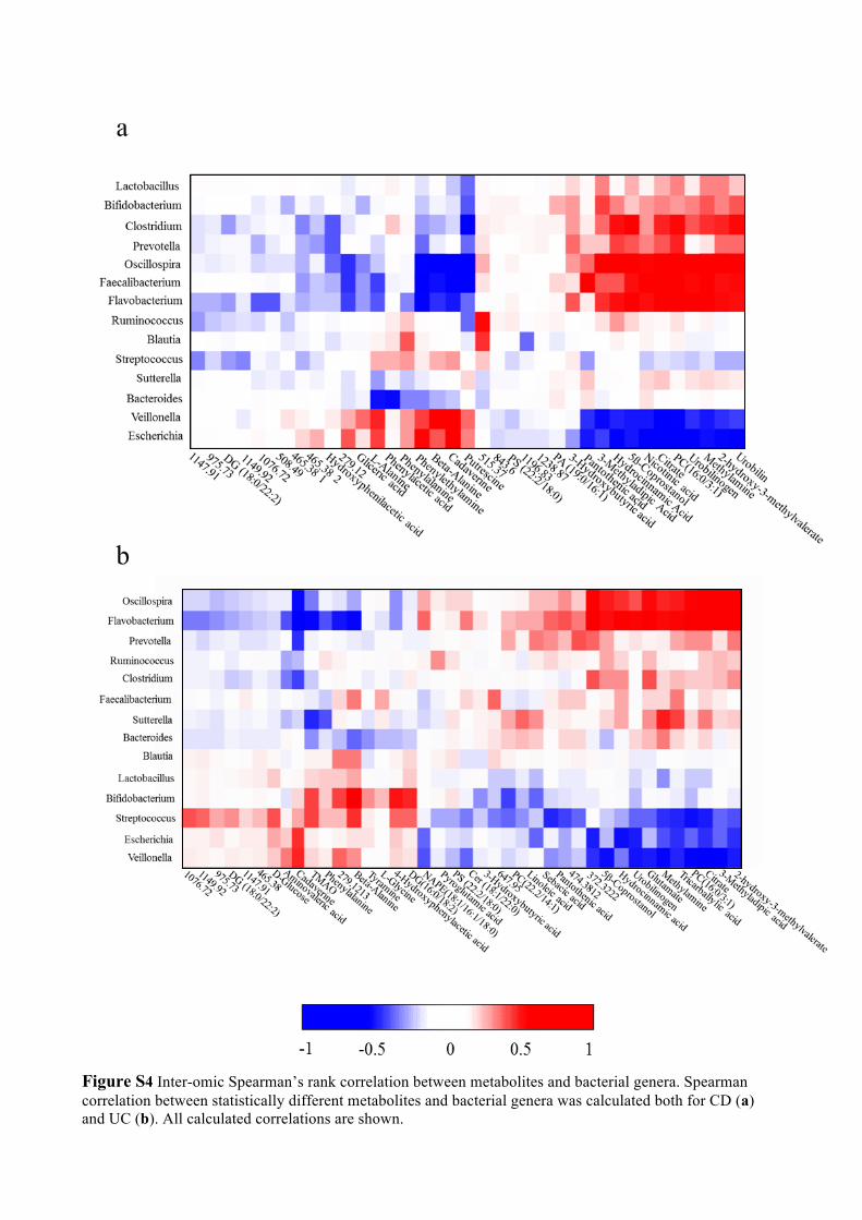
Figure S4 Inter-omic Spearman’s rank correlation between metabolites and bacterial genera. Spearman correlation between statistically different metabolites and bacterial genera was calculated both for CD (a) and UC (b). All calculated correlations are shown.

Figure S5 Inter-omic Spearman’s rank correlation between metabolites and bacterial species. Spearman correlation between statistically different metabolites and bacterial species was calculated both for CD (a) and UC (b). All calculated correlations are shown.

References

1. Gregory KE, Bird SS, Gross VS, et al. Method development for fecal lipidomics profiling. Anal Chem 2012;85(2):1114-23.

2. R Core Team. R: A language and environment for statistical computing. R Foundation for Statistical Computing. 2011. http://www.R-project.org/.

3. Smith CA, Want EJ, O'Maille G, Abagyan R, et al. XCMS: processing mass spectrometry data for metabolite profiling using nonlinear peak alignment, matching, and identification. Anal Chem 2006;78:779-87.

4. Libiseller G, Dvorzak M, Kleb U, et al. IPO: a tool for automated optimization of XCMS parameters. BMC bioinformatics 2015;16:118.

5. Kuhl C, Tautenhahn R, Böttcher C, et al. CAMERA: an integrated strategy for compound spectra extraction and annotation of liquid chromatography/mass spectrometry data sets. Anal Chem 2012; 84:283-89.

6. Veselkov KA, Vingara LK, Masson P, et al. Optimized preprocessing of ultra-performance liquid chromatography/mass spectrometry urinary metabolic profiles for improved information recovery, Anal Chem 2011;83:5864-72.