HAL Id: hal-00845446https://hal.archives-ouvertes.fr/hal-00845446v2

Preprint submitted on 21 May 2014

HAL is a multi-disciplinary open accessarchive for the deposit and dissemination of sci-entific research documents, whether they are pub-lished or not. The documents may come fromteaching and research institutions in France orabroad, or from public or private research centers.

L’archive ouverte pluridisciplinaire HAL, estdestinée au dépôt et à la diffusion de documentsscientifiques de niveau recherche, publiés ou non,émanant des établissements d’enseignement et derecherche français ou étrangers, des laboratoirespublics ou privés.

Crossed-Derivative Based Sensitivity Measures forInteraction Screening

Olivier Roustant, Jana Fruth, Bertrand Iooss, Sonja Kuhnt

To cite this version:Olivier Roustant, Jana Fruth, Bertrand Iooss, Sonja Kuhnt. Crossed-Derivative Based SensitivityMeasures for Interaction Screening. 2014. �hal-00845446v2�

Crossed-Derivative Based Sensitivity Measures for

Interaction Screening

O. Roustanta,∗, J. Fruthb, B. Ioossc, S. Kuhntb,d

aEcole Nat. Sup. des Mines, FAYOL-EMSE, LSTI, F-42023 Saint-Etienne, FrancebFaculty of Statistics, TU Dortmund University, Vogelpothsweg 87, 44227 Dortmund,

GermanycElectricite de France R&D, 6 quai Watier, F-78401, France

dDepartment of Computer Science, Dortmund University of Applied Sciences and Arts,

Emil-Figge-Strasse 42, 44227 Dortmund, Germany

Abstract

Global sensitivity analysis is used to quantify the influence of input variableson a numerical model output. Sobol’ indices are now classical sensitivitymeasures. However their estimation requires a large number of model eval-uations, especially when interaction effects are of interest. Derivative-basedglobal sensitivity measures (DGSM) have recently shown their efficiency forthe identification of non-influential inputs. In this paper, we define crossedDGSM, based on second-order derivatives of model output. By using a L2-Poincare inequality, we provide a crossed-DGSM based maximal bound forthe superset importance (i.e. total Sobol’ indices of an interaction betweentwo inputs). In order to apply this result, we discuss how to estimate thePoincare constant for various probability distributions. Several analyticaland numerical tests show the performance of the bound and allow to developa generic strategy for interaction screening.

Keywords: Sensitivity analysis, Derivative-based sensitivity measure,Sobol decomposition, Interactions, Superset importance, Additive structure

∗Corresponding author: roustant@emse.fr, Phone: +33 477426675, Fax: +33477426666

Email addresses: fruth@statistik.tu-dortmund.de (J. Fruth),bertrand.iooss@edf.fr (B. Iooss), sonja.kuhnt@fh-dortmund.de (S. Kuhnt)

Preprint submitted to Elsevier May 21, 2014

1. Introduction

In engineering studies, computer models simulating physical phenomenaand industrial systems often take as inputs a high number of numerical andphysical variables. For the development, the analysis and the uses of suchcomputer models, the global sensitivity analysis methodology is an invalu-able tool [22]. Among quantitative methods, variance-based methods areused most often [23]. The main idea of these methods is to evaluate, bythe way of so-called Sobol indices [24], how the variation of an input or agroup of inputs contributes to the model output variability. Sobol indices offirst order measure the effect of individual inputs, while second-order Sobolindices correspond to the influence of the interaction between two inputs(by excluding their individual effects). Moreover, the powerful total Sobolsensitivity index has been introduced to express the overall contribution ofone specified input, including the effects of its interactions (second order,third order, . . . ) with all the other inputs [11]. More generally, the so-calledsuperset importance of an input set I has been defined in [17] and [12] asthe sum of all Sobol’ indices relative to the supersets of I. In the particularcase of two inputs, the superset importance has been referred to as the totalinteraction index ([8]). When its value is zero, it means that there is nointeraction term containing simultaneously the two inputs. By analogy withscreening, this can be viewed as interaction screening.

However, obtaining all these Sobol sensitivity indices is rather costly interms of the number of necessary model evaluations [23]. This seriously lim-its their use because industrial computer codes often require several minutesor hours to perform one run. Moreover, for large dimension (number of in-puts larger than several tens), high-order Sobol’ indices cannot be obtainedby non-costly alternative methods based on metamodels or smoothing tech-niques [29, 18]. Introduced by [26], an alternative global sensitivity estimatorconsists, for each input, in integrating the square derivative of the model out-put over the domain of the inputs. Called later the Derivative-based GlobalSensitivity Measures (DGSM), they have been proved to be computationallymore tractable than variance-based measures [15], allowing to manage theproblem of large numbers of inputs. DGSM have only been finely studiedand applied recently [27, 21, 13]. Moreover, these indices need the computa-tion of the gradient of the model output with respect to the model inputs,which can be at least estimated by a finite-differences technique. However, ifthe computer model proposes the adjoint code to compute output derivatives

2

[5], DGSM computations will be independent of the number of input param-eters and sensitivity analysis can then be performed for models includingseveral hundreds of inputs. Automatic differentiation tools [9] can be helpfulto that purpose.

Recently, some authors have discovered links between DGSM and variance-based sensitivity indices. For an input following a uniform or normal proba-bility distribution, [27] has proved that the total Sobol’ index is bounded by aterm involving a constant and the DGSM. [16] has developed a generalizationof this inequality for a large class of continuous probability measures. Thus,it has been proved that the DGSM can be used for robust variable screen-ing. In engineering applications, this inequality allows to develop a genericstrategy to obtain global sensitivity information from DGSM and first-orderSobol indices [13].

In this paper we extend this approach to interactions, by proving a gener-alization of the inequality in the same large class of probability measures. Wealso obtain results for the class of log-concave measures. Thus, the second-order derivatives contained in the Hessian of the model output are useful toinvestigate interactions. Such a link was investigated for instance by [7] in thecontext of statistical learning, but the connection to superset indices givesan original interpretation of it. While it is rare in practice that second-orderderivatives of the model output are directly available, they can be computedby second-order finite differences or by automatic differentiation tools. Inthe same vein of [16], we also investigate by numerical tests the utility of theinequality in ranking the most influential interactions. While this rankingmay be useful at first sight for superset importances more than for second-order interactions, we can argue that in practice it is very often the case thatsecond-order interactions are the only active ones.

In [28], a similar problem has been considered by using groups of inputs.The same kind of inequality links the total Sobol index of a group with thecorresponding DGSM (equal to the integral of the square sum of the partialderivatives of each group input). If this latter measure is zero, it means thatthere is no interaction between the inputs inside the group. However, if theDGSM of a group is non zero, the total interaction index between two inputscan be zero, which is detected by the crossed DGSM.

The paper is organized as follows: Section 2 recalls some useful defini-tions of sensitivity indices (Sobol indices, superset importances, DGSM) andintroduces the crossed DGSM. Section 3 establishes an inequality betweensuperset importance and crossed DGSM. Section 4 focuses on the determi-

3

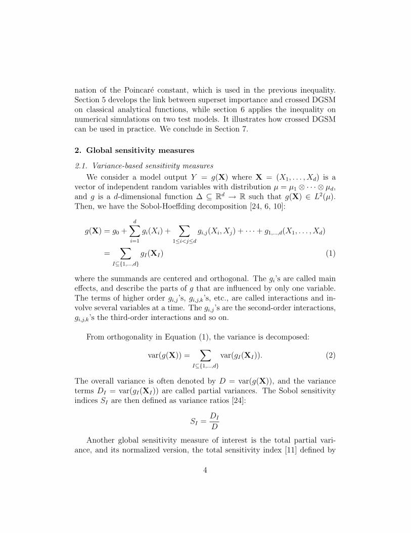
nation of the Poincare constant, which is used in the previous inequality.Section 5 develops the link between superset importance and crossed DGSMon classical analytical functions, while section 6 applies the inequality onnumerical simulations on two test models. It illustrates how crossed DGSMcan be used in practice. We conclude in Section 7.

2. Global sensitivity measures

2.1. Variance-based sensitivity measures

We consider a model output Y = g(X) where X = (X1, . . . , Xd) is avector of independent random variables with distribution µ = µ1 ⊗ · · · ⊗ µd,and g is a d-dimensional function ∆ ⊆ R

d → R such that g(X) ∈ L2(µ).Then, we have the Sobol-Hoeffding decomposition [24, 6, 10]:

g(X) = g0 +d∑

i=1

gi(Xi) +∑

1≤i<j≤d

gi,j(Xi, Xj) + · · · + g1,...,d(X1, . . . , Xd)

=∑

I⊆{1,...,d}

gI(XI) (1)

where the summands are centered and orthogonal. The gi’s are called maineffects, and describe the parts of g that are influenced by only one variable.The terms of higher order gi,j’s, gi,j,k’s, etc., are called interactions and in-volve several variables at a time. The gi,j’s are the second-order interactions,gi,j,k’s the third-order interactions and so on.

From orthogonality in Equation (1), the variance is decomposed:

var(g(X)) =∑

I⊆{1,...,d}

var(gI(XI)). (2)

The overall variance is often denoted by D = var(g(X)), and the varianceterms DI = var(gI(XI)) are called partial variances. The Sobol sensitivityindices SI are then defined as variance ratios [24]:

SI =DI

D

Another global sensitivity measure of interest is the total partial vari-ance, and its normalized version, the total sensitivity index [11] defined by

4

considering the supersets of sets of size 1:

DTi =

∑

J⊇{i}

DJ , STi =

DTi

D. (3)

The total indices allow to detect unessential variables: If DTi = 0 then g(x)

does not depend on xi. An extension to general supersets was proposed by[12, 17], who defined the superset importance:

DsuperI =

∑

J⊇I

DJ , SsuperI =

DsuperI

D, (4)

where I ⊆ {1, . . . , d}. In the case of a pair of variables {Xi, Xj}, we have:Dsuper

i,j =∑

I⊇{i,j} DI .

2.2. DGSM and crossed DGSM

Motivated by the reduction of computational cost, [15] proposed to usethe derivative-based global sensitivity measures (DGSM):

νi =

∫ (∂g(x)

∂xi

)2

dµ(x). (5)

In the equation above it is assumed that g admits a weak directional deriva-tive (i.e. in the sense of distributions) with respect to xi such that ∂g(X)

∂xi∈

L2(µ). The DGSM play a similar role to total indices in detecting unessentialvariables: If νi = 0 then g(x) does not depend on xi.

Investigating interactions, [7] used the integral of squared crossed deriva-tives. For second-order interactions, they introduced (assuming similar con-ditions on the higher-order derivatives of g):

νi,j =

∫ (∂2g(x)

∂xi∂xj

)2

dµ(x), (6)

and more generally, for I ⊆ {1, . . . , d}:

νI =

∫ (∂|I|g(x)

∂xI

)2

dµ(x),

with ∂xI =∏

i∈I ∂xi, and |I| is the size of I. By analogy to DGSM, when|I| ≥ 2 we propose to call the quantities νI crossed DGSM.

5

2.3. Utilization of superset importance and crossed DGSM

Superset importance and crossed DGSM are both useful in order to in-vestigate interactions, and discover additive structures in g. In practice, themost useful case is for a pair of indices {i, j}. If either νi,j = 0 or Dsuper

i,j = 0,then g can be written as a sum of two functions, one that does not dependon xi and the other that does not depend on xj [12, 7]:

g(x) = g−i(x−i) + g−j(x−j)

Equivalently, this means that Xi and Xj do not interact together, nor to-gether with other variables: ∀I ⊇ {i, j} : DI = 0. In particular – and this isweaker in general – it implies that Di,j = 0.

2.4. First-order analysis, second-order analysis. FANOVA graph.

In applications it is reasonable to perform sequentially so-called first-order and second-order analysis. The first-order analysis considers singleinputs and aims at detecting the non-influential ones, i.e. the Xi’s for whichST

i = 0. First-order sensitivity indices are computed, as well as total sensitiv-ity indices or DGSMs. The second-order analysis considers pairs of inputs,and aims at detecting the non-influential interactions, i.e. the pairs {i, j}for which Ssuper

i,j = 0. This can be used to detect additive structures (see theprevious section). Superset importance or crossed DGSMs are computed.The second-order analysis may generate a large amount of information cor-responding to the number of input pairs p(p − 1)/2, where p is the problemdimension. Actually p can be lowered to the number of influential variables.Indeed, if Xi is non-influential, it does not contribute to the output, neitherindividually nor in interaction with another input, and thus Ssuper

i,j = νi,j = 0for all j. Such information is conveniently visualized by the way of theso-called FANOVA graph [19], where vertices represent inputs, and edges in-dicate the presence of interactions involving two inputs simultaneously. Theedges widths can then be chosen proportionally to the quantity of interest.

3. A link between superset importance and crossed DGSM

In what follows, we consider a class of distributions that satisfy a Poincareinequality: ∫

g(x)2dµ(x) ≤ C(µ)

∫‖∇g(x)‖2dµ(x) (7)

6

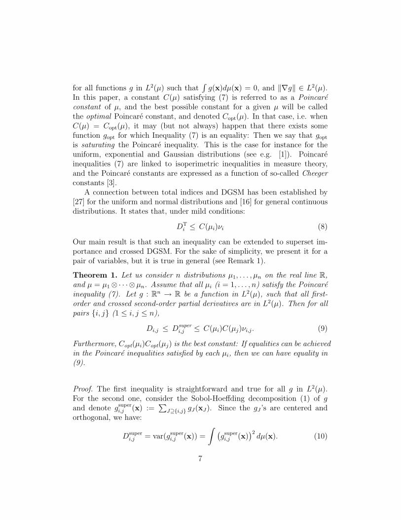
for all functions g in L2(µ) such that∫

g(x)dµ(x) = 0, and ‖∇g‖ ∈ L2(µ).In this paper, a constant C(µ) satisfying (7) is referred to as a Poincareconstant of µ, and the best possible constant for a given µ will be calledthe optimal Poincare constant, and denoted Copt(µ). In that case, i.e. whenC(µ) = Copt(µ), it may (but not always) happen that there exists somefunction gopt for which Inequality (7) is an equality: Then we say that gopt

is saturating the Poincare inequality. This is the case for instance for theuniform, exponential and Gaussian distributions (see e.g. [1]). Poincareinequalities (7) are linked to isoperimetric inequalities in measure theory,and the Poincare constants are expressed as a function of so-called Cheegerconstants [3].

A connection between total indices and DGSM has been established by[27] for the uniform and normal distributions and [16] for general continuousdistributions. It states that, under mild conditions:

DTi ≤ C(µi)νi (8)

Our main result is that such an inequality can be extended to superset im-portance and crossed DGSM. For the sake of simplicity, we present it for apair of variables, but it is true in general (see Remark 1).

Theorem 1. Let us consider n distributions µ1, . . . , µn on the real line R,and µ = µ1 ⊗· · ·⊗µn. Assume that all µi (i = 1, . . . , n) satisfy the Poincareinequality (7). Let g : R

n → R be a function in L2(µ), such that all first-order and crossed second-order partial derivatives are in L2(µ). Then for allpairs {i, j} (1 ≤ i, j ≤ n),

Di,j ≤ Dsuper

i,j ≤ C(µi)C(µj)νi,j. (9)

Furthermore, Copt(µi)Copt(µj) is the best constant: If equalities can be achievedin the Poincare inequalities satisfied by each µi, then we can have equality in(9).

Proof. The first inequality is straightforward and true for all g in L2(µ).For the second one, consider the Sobol-Hoeffding decomposition (1) of gand denote gsuper

i,j (x) :=∑

J⊇{i,j} gJ(xJ). Since the gJ ’s are centered andorthogonal, we have:

Dsuperi,j = var(gsuper

i,j (x)) =

∫ (gsuper

i,j (x))2

dµ(x). (10)

7

Furthermore we have: ∂2g(x)∂xi∂xj

=∂2gsuper

i,j(x)

∂xi∂xj, since all terms in (1) that do not

contain simultaneously xi and xj vanish by cross derivation. This leads to:

νi,j =

∫ (∂2gsuper

i,j (x)

∂xi∂xj

)2

dµ(x). (11)

The result then follows from a sequential application of 1-dimensional Poincareinequalities. Indeed, let us first fix all variables except xi. Then:

∫ (gsuper

i,j (x))2

dµi(xi) ≤ C(µi)

∫ (∂gsuper

i,j (x)

∂xi

)2

dµi(xi).

Similarly, fixing all variables except xj and considering∂gsuper

i,j(x)

∂xi, we have:

∫ (∂gsuper

i,j (x)

∂xi

)2

dµj(xj) ≤ C(µj)

∫ (∂

∂xj

∂gsuperi,j (x)

∂xi

)2

dµj(xj).

Then, integrating and combining the two inequalities above gives, togetherwith (10) and (11), the announced inequality.Finally, to see that Copt(µi)Copt(µj) is the best constant, suppose that foreach µk, (7) is saturated with a centered function gk

opt:

∫gkopt(t)

2dµk(t) = Copt(µk)

∫[(gk

opt)′(t)]2dµk(t).

Then a direct computation shows that we have equality in (9) with g(xi, xj) =giopt(xi)g

jopt(xj):

Di,j = Dsuperi,j = Copt(µi)Copt(µj)νi,j.

Remark also that g(x) =∑

k,ℓ gkopt(xk)g

ℓopt(xℓ) achieves equality in (9) simul-

taneously for all pairs {i, j}.

Remark 1. A similar proof can be used to show that for a general subset I,we have: Dsuper

I ≤ ∏i∈I C(µi)νI .

4. Computation of Poincare constants on the real line

In Theorem 1, we can see that Inequality (9) involves only Poincare con-stants on the real line (namely the C(µi)’s). There exists an abundant liter-ature on that topic, and some pointers are given in [1]. Here, following [16],

8

we assume that µ is continuous (absolutely continuous with respect to theLebesgue measure) and focus on some practical results to compute Poincareconstants. We denote by f the probability density function, F its cumula-tive density function, and q the quantile function. Finally m = q(0.5) is themedian.

First of all, there are at least two cases where optimal constants areknown: The uniform and normal distributions (see e.g. [27] or [1]). Theconstants are given in Table 1.

Distribution Optimal Poincare constant A case of equality

Uniform U [a, b] (b − a)2/π2 g(x) = cos(

π(x−a)b−a

)

Normal N (µ, σ2) σ2 g(x) = x − µ

Table 1: Optimal Poincare constants for the uniform and normal distributions.

In general, however, optimal constants are not available. Fortunatelyuseful Poincare constants can be derived for some classes of distributions,including in particular log-concave distributions [20].

Definition 1. (log-concave distribution) A continuous distribution µ is calledlog-concave if log(f) is concave.

Three main results are summarized in Table 2. The first one is commonto all continuous distributions, and can be found in [4, 3]. It gives a Poincareconstant that can be computed numerically by maximizing a 1-dimensionalfunction. For log-concave distributions, this maximum has an analyticalexpression [3], Section 4, and several examples are given in [16] includingexponential, Gumbel and Weibull distributions. The last result – useful inapplications – is derived for truncated distributions (for a proof see AppendixA).

Remark 2. (Isoperimetric, Cheeger and Poincare constants). Due to theinterpretation of Poincare inequalities as isoperimetric inequalities [3], thereare several constants that are closely linked to each other. The quantityIs(µ) := inf

x∈R

f(x)min(F (x),1−F (x))

is called isoperimetric constant [4]. Its inverse

1/Is(µ) is often called Cheeger constant [16]. Then C(µ) = 4/Is(µ)2 is aPoincare constant for the distribution µ (see [3]), as reported in Table 2.

9

Properties of µ A Poincare constant C(µ)

Continuous 4

[supx∈R

min(F (x),1−F (x))f(x)

]2

log-concave 1/f(m)2

log-concave, truncated on [a, b] (F (b) − F (a))2 /f(q(

F (a)+F (b)2

))2

Table 2: Example of (non-optimal) Poincare constants for some classes of continuousdistributions.

Remark 3. (Boltzmann distributions and erratum in [16]). Continuous dis-tributions dµ(x) = f(x)dx are sometimes expressed as Boltzmann distri-butions: f(x) = c exp[−v(x)]1∆(x), where c is a (non-unique) normalizingconstant and ∆ = {x ∈ R, f(x) 6= 0}. If f is log-concave, then the Poincareconstant of Table 2 is equal to 1/f(m)2 = exp[2v(m)]/c2, and the corre-sponding Cheeger constant (as defined in Remark 2) to exp[v(m)]/(2c). Thenormalizing constant c is sometimes missing in the text of [16]: In Theo-rem 3.2. (c was omitted in the denominator) and in Table 2, first line: Oneshould read σ/2 ×

√2π.

5. Examples for usual analytical functions

5.1. Second order polynomials

Consider a second-order polynomial given by its ANOVA decomposition:

g(X) = β0 +d∑

i=1

βi(Xi − mi) +∑

1≤i<j≤d

βi,j(Xi − mi)(Xj − mj),

where mi = E(Xi), 1 ≤ i ≤ d. Then we have immediately:

Dsuperi,j = Di,j = (βi,j)

2var(Xi)var(Xj), νi,j = (βi,j)2.

Thus, contrarily to superset importance, the crossed DGSM do not dependon the distribution of the Xk’s but only on the coefficients of the second-orderterms. Consequently, they can give only a rough indication of the interactionsimportance, but that indication is sufficient to detect the unessential ones:νi,j = 0 ⇔ Di,j = 0 (assuming that var(Xi) > 0, var(Xj) > 0).

10

5.2. Functions with separated variables

Following [27], let us consider

g(X) =d∏

i=1

ϕi(Xi),

where ϕi(Xi) and ϕ′i(Xi) are in L2(µi). By denoting Ai =

∫ϕi(t)dµi(t) and

introducing the centered function ϕi,0(.) = ϕi(.) − Ai, this is rewritten as:

g(X) =d∏

i=1

(Ai + ϕi,0(Xi)),

and the ANOVA decomposition of g is obtained by expanding the product(see [25]) and gI(XI) =

∏j /∈I Aj

∏i∈I ϕi,0(Xi). Then a direct computation

shows that:

Dsuperi,j =

∏

k/∈{i,j}

(A2k + Bk) BiBj νi,j =

∏

k/∈{i,j}

(A2k + Bk) B′

iB′j

with Bi :=∫

ϕ2i,0(t)dµi(t) and B′

i :=∫

[ϕ′i,0(t)]

2dµi(t). In particular for anon-zero interaction, we have:

νi,j

Dsuperi,j

=B′

i

Bi

B′j

Bj

. (12)

This generalizes the formula given in [27] for first-order indices:

νi

DTi

=B′

i

Bi

.

Their examples with uniform distributions on [0, 1] are also immediately ex-tended:

• For the g-function g(x) =∏d

i=1(|4xi − 2| + ai)/(1 + ai), the ratio isconstant:

νi,j

Dsuper

i,j

= 482, and much larger than π2, the bound given by

the optimal Poincare constant.

• Choosing ϕi(t) = tm, ϕj(t) = tn leads toνi,j

Dsuper

i,j

≈ (m + 1)2(n + 1)2 for

large m and n, and the ratio can be arbitrary large.

11

6. Numerical examples and applications

The aim of this section is to illustrate how DGSM and crossed DGSMcan be used in practice. More precisely, the analysis should be based on theirupper bounds, denoted by Ui and Ui,j, obtained with Inequalities (8) and (9):

Ui := C(µi)νi

D≥ ST

i (13)

Ui,j := C(µi)C(µj)νi,j

D≥ Ssuper

i,j (14)

In the following, we consider analytical examples and a case study. We per-form sequentially first-order analysis in order to detect influential inputs, anda second-order analysis in order to study interactions and discover additivestructures, as detailed in Section 2.4. These two analyses imply the estima-tion of various sensitivity indices. The estimation of variance-based sensitiv-ity indices has been intensively studied since Sobol’ formula for closed indices[24]. For total indices and superset importance, two useful formulas can beused, due to [14] and [17]:

DTi =

1

2

∫[f(x) − f(zi,x−i)]

2 dµ(x)dµi(zi) (15)

Dsuperi,j =

1

4

∫[f(x) − f(xi, zj,x−i,j)

−f(zi, xj,x−i,j) + f(zi, zj,x−i,j)]2 dµ(x)dµi(zi)dµj(zj) (16)

Accurate estimators are derived by using Monte Carlo estimates of the inte-grals above. They share good properties, studied in [8]: They are positive,unbiased and asymptotically efficient. Furthermore, they are identically zeroif the “true” index is zero.For DGSM and crossed DGSM, estimations are obtained by using also MonteCarlo estimates of the integrals in Equations (5) and (6). In addition, thederivatives should be replaced by finite differences when the gradient and/orHessian are not supplied. In this section, we use finite differences. In bothcases, it is easy to see that the estimators share the same property as above:They are identically zero if the true index is zero.Finally, notice that all the integrals could be replaced by Quasi-Monte Carloestimates rather than Monte Carlo ones, but this is beyond the scope of thepresent paper.

12

Remark 4. Formula (16) contains a crossed finite difference inside thesquare. It is thus very similar to the crossed DGSM definition (6). Thiscan be used to prove Inequality (9) from (16), as detailed in Appendix B.

6.1. Analytical examples

6.1.1. Ishigami function

The Ishigami function is a popular toy example in sensitivity analysis,due to the presence of non-linearities and a strong (non-linear) interaction.It is defined on ∆ = [−π, π]3 by:

f(x1, x2, x3) = sin(x1) + 7 sin(x2)2 + 0.1x4

3 sin(x1).

We consider f(X1, X2, X3), assuming that X1, X2, X3 are independent ran-dom variables from the uniform distribution on [−π, π]. Each index is es-timated a 100 times on different Monte Carlo samples of size 1000. Theresulting mean and standard deviation values of the sensitivity analysis arereported in Tables 3 and 4. The theoretical values, here calculable, are alsoindicated. We observe that the upper bounds are quite large, though theoptimal Poincare constant was used. No major conclusion is obtained fromTable 3, since all inputs are influential. We see, however, that the rankingof inputs is different whether it is based on ST

i or Ui. The second-orderanalysis (Table 4) shows that the non-influential interactions {2, 1}, {2, 3}are correctly detected by the Ui,j’s. Notice that the estimation is exactlyzero when the index is zero, a property of the Liu and Owen’s estimator (seeabove). This implies that there are no interactions (at any order) involvingboth X2 and X1, and no interactions (at any order) involving both X3 andX1, revealing an additive structure for f :

f(x1, x2, x3) = f1,3(x1, x3) + f2(x2)

Input Si STi m(ST

i ) sd(STi ) Ui m(Ui) sd(Ui)

X1 0.314 0.558 0.558 (0.047) 2.230 2.234 (0.146)X2 0.442 0.442 0.442 (0.015) 7.079 7.048 (0.163)X3 0 0.244 0.243 (0.016) 3.174 3.213 (0.221)

Table 3: First-order analysis for the Ishigami function (uniform inputs). Upper boundsare computed with Copt(µ) = 4. Standard deviations are obtained with 100 replicates.

13

Input pair Si,j Ssuperi,j m(Ssuper

i,j ) sd(Ssuperi,j ) Ui,j m(Ui,j) sd(Ui,j)

X1 : X2 0 0 0 (0) 0 0 (0)X1 : X3 0.244 0.244 0.241 (0.020) 12.698 12.686 (0.828)X2 : X3 0 0 0 (0) 0 0 (0)

Table 4: Second-order analysis for the Ishigami function (uniform inputs). Upper boundsare computed with Copt(µ) = 4. Standard deviations are obtained with 100 replicates.

6.1.2. A 6-dimensional block-additive function

Following [19], we consider the 6-dimensional function in L2:

a(X1, . . . , X6) = cos([1, X1, X5, X3]φ) + sin([1, X4, X2, X6]γ)

with φ = [−0.8,−1.1, 1.1, 1]T , γ = [0.5, 0.9, 1,−1.1]T , and where X1, . . . , X6

are assumed independent and uniformly distributed on ∆ = [−1, 1]6. Theresults for sensitivity analysis are reported in Tables 5 and 6. Again eachestimation is performed with a Monte Carlo sample of size 1000 and repeated100 times. Table 5 shows that all variables are influential, either by lookingat ST

i or Ui. Looking at interactions between pairs of inputs, Table 6 clearlydetects inactive interactions, either by looking at Ssuper

i,j or Ui,j. Again, the es-timation is exactly zero when the index is zero. The corresponding FANOVAgraphs (see 2.4) are represented in Figure 1, which are very similar here. Twogroups are visible: {1, 3, 5} and {2, 4, 6}, meaning that there are no interac-tions (at any order) between Xi and Xj when i belongs to the first group,and j to the second one. Thus the Sobol-Hoeffding decomposition (1) impliesthat the ‘a’ function has the block-additive form:

a(X1, . . . , X6) = a1,3,5(X1, X3, X5) + a2,4,6(X2, X4, X6)

which is the correct structure of the ‘a’ function.

6.2. A case study

We consider the flood model presented in [16]. The output is the maximalannual overflow (in meters), denoted by S:

S = Zv + H − Hd − Cb with H =

Q

BKs

√Zm−Zv

L

0.6

,

14

Input Si STi m(ST

i ) sd(STi ) Ui m(Ui) sd(Ui)

X1 0.110 0.231 0.231 (0.012) 0.329 0.329 (0.007)X2 0.143 0.214 0.215 (0.009) 0.285 0.285 (0.005)X3 0.086 0.196 0.197 (0.010) 0.272 0.272 (0.006)X4 0.112 0.176 0.176 (0.008) 0.231 0.231 (0.004)X5 0.110 0.231 0.232 (0.011) 0.329 0.329 (0.007)X6 0.180 0.256 0.256 (0.011) 0.345 0.345 (0.007)

Table 5: First-order analysis for the ‘a’ function (uniform inputs). Upper bounds arecomputed with Copt(µ) = 4/π2. Standard deviations are obtained with 100 replicates.

Input pair Si,j Ssuperi,j m(Ssuper

i,j ) sd(Ssuperi,j ) Ui,j m(Ui,j) sd(Ui,j)

X1 : X2 0 0 0 (0) 0 0 (0)X1 : X3 0.043 0.067 0.067 (0.005) 0.133 0.132 (0.003)X1 : X4 0 0 0 (0) 0 0 (0)X1 : X5 0.055 0.078 0.080 (0.006) 0.161 0.160 (0.004)X1 : X6 0 0 0 (0) 0 0 (0)X2 : X3 0 0 0 (0) 0 0 (0)X2 : X4 0.018 0.040 0.039 (0.004) 0.085 0.085 (0.002)X2 : X5 0 0 0 (0) 0 0 (0)X2 : X6 0.031 0.053 0.052 (0.005) 0.127 0.127 (0.003)X3 : X4 0 0 0 (0) 0 0 (0)X3 : X5 0.043 0.067 0.067 (0.005) 0.133 0.132 (0.003)X3 : X6 0 0 0 (0) 0 0 (0)X4 : X5 0 0 0 (0) 0 0 (0)X4 : X6 0.024 0.046 0.045 (0.004) 0.103 0.103 (0.002)X5 : X6 0 0 0 (0) 0 0 (0)

Table 6: Second-order analysis for the ‘a’ function (uniform inputs). Upper bounds arecomputed with Copt(µ) = 4/π2. Standard deviations are obtained with 100 replicates.

where H is the maximal annual height of the river (in meters). The 8 inputsare assumed to be independent random variables, with distributions recalledin Table 7.

The first-order analysis was performed in [16], and 3 nonessential inputswere detected. We base the second-order analysis on the 5 remaining ones:X1 = Q, X2 = Ks, X3 = Zv, X5 = Hd, X6 = Cb. We fix the non-influentialinputs at their mean value and estimate the Ssuper

i,j and Ui,j using a Monte

15

12

3

4

5

6

12

3

4

5

6

Figure 1: FANOVA graphs of Ssuper

i,j (left) and Ui,j (right) for the ‘a’ function.

Input Description Unit Probability distributionX1 = Q Maximal annual flowrate m3/s Gumbel G(1013, 558),

truncated on [500, 3000]X2 = Ks Strickler coefficient - Normal N (30, 8),

truncated on [15, +∞[X3 = Zv River downstream level m Triangular T (49, 50, 51)X4 = Zm River upstream level m Triangular T (54, 55, 56)X5 = Hd Dyke height m Uniform U [7, 9]X6 = Cb Bank level m Triangular T (55, 55.5, 56)X7 = L River stretch m Triangular

T (4990, 5000, 5010)X8 = B River width m Triangular T (295, 300, 305)

Table 7: Input variables of the flood model and their probability distributions.

Carlo sample size of 20,000. The true amount of variance explained by in-teractions is here very small, around 1%. The results are reported in Table8 and visualized on Figure 2. Departures are visible between the resultsobtained with variance-based sensitivity indices and derivative-based ones.One reason is that the Poincare constants used are not optimal, and do nothave the same order of magnitude. In particular one of them is very largedue to the fat tail of the Gumbel distribution. Consequently we see that theupper bounds are rather rough. The second-order analysis based on crossedDGSMs succeeds in detecting the nonessential interactions, after inspecting

16

Table 8. However this result must be considered with much care here, sinceit also corresponds to low values of Poincare constants products. Similarlywe are very lucky here to rank at first place the most influential interaction,corresponding to the highest product C(µi)C(µj).

Finally, we consider the second output, a cost estimation, proposed in[16]. The same 5 inputs are influential and again the interaction indicesare estimated on a Monte Carlo size of 20,000.. The true amount of varianceexplained by the interactions is about 10%. The second-order analysis clearlyshows a difference in ranking, as shown in Figure 3. This may be due eitherto the form of the function considered, or to the heterogeneity of distributionsas explained above. Notice however that crossed DGSM conclude correctlyto the absence of non-influential interactions.

Ssuperi,j Ui,j C(µi)C(µj)

X1 : X2 0.008235 1.837809 819887392.342X1 : X3 0.000178 0.011691 2165585.265X1 : X5 0.000000 0.001947 877678.649X1 : X6 0.000000 0.000000 541396.316X2 : X3 0.000070 0.003758 378.599X2 : X5 0.000000 0.000000 153.440X2 : X6 0.000000 0.000000 94.650X3 : X5 0.000000 0.000000 0.405X3 : X6 0.000000 0.000000 0.250X5 : X6 0.000000 0.000000 0.101

Table 8: Second-order analysis for the overflow output of the flood model, limited to theinfluential inputs.

7. Conclusion

This paper focuses on the quantification of interactions in global sensi-tivity analysis. We considered the integral of squared crossed derivativesintroduced in statistical learning [7], that we call crossed DGSM by analogyto DGSM [26]. We show that there is a Poincare-type inequality betweensuperset importance [17] and the crossed DGSM. This extends to interactionthe link between total effects and DGSM [27, 16].

17

1

2

3

5

6

1

2

3

5

6

Figure 2: FANOVA graphs of Ssuper

i,j (left) and Ui,j (right) for the overflow output of theflood model, limited to the influential inputs.

1

2

3

5

6

1

2

3

5

6

Figure 3: FANOVA graphs of Ssuper

i,j (left) and Ui,j (right) for the cost output of the floodmodel, limited to the influential inputs.

This new inequality can be used to detect additive structures in black-boxfunctions by detecting pairs of inputs that do not interact together (see[12, 19, 8]). We investigated their practical utilization with two analyticalexamples involving uniform inputs and one case study with several hetero-geneous input distributions. For that purpose, we recalled some facts aboutPoincare inequalities, and gave a new expression of a Poincare constant fortruncated log-concave distributions. The crossed DGSM performed well inthe examples, for which the optimal Poincare constant is known. In particu-lar, the additive structure of a 6-dimensional function was recovered. On theother hand, the case study showed some limitations of the crossed DGSM,

18

also shared by the usual DGSM (see [27] for a discussion). In particular,some Poincare constants used are not optimal and sometimes very large, andthe inequality was not informative for several pairs of inputs. In such cases,an idea for future research could be to investigate the use of transformationsof the inputs into uniformly or normally distributed ones, which simplifiesthe input distributions but may introduce undesirable non-linearities in thenew function obtained by composition.

Acknowledgements

Parts of this work have been backed by French National Research Agency(ANR) through COSINUS program (project COSTA BRAVA noANR-09-COSI-015), or conducted within the frame of the ReDice Consortium, gath-ering industrial (CEA, EDF, IFPEN, IRSN, Renault) and academic (Ecoledes Mines de Saint-Etienne, INRIA, and the University of Bern) partnersaround advanced methods for Computer Experiments. The financial sup-port of the DFG (SFB708: Project C3) is also gratefully acknowledged. Wethank Fabrice Gamboa and Franck Barthe for helpful discussions.

Appendix A. Poincare constants for truncated log-concave distri-butions.

Proposition 1. Let µ be a log-concave distribution. Let a, b be two realnumbers such that −∞ ≤ a < b ≤ +∞, and consider the truncated distri-bution µa,b defined on [a, b] by its cdf Fa,b(x) = F (x)−F (a)

F (b)−F (a)1[a,b](x), where 1[a,b]

denotes the indicator function. Then µa,b satisfies a Poincare inequality with

C(µa,b) = (F (b) − F (a))2 /f(q(

F (a)+F (b)2

))2

.

Proof. As a truncation of a log-concave distribution, µa,b is log-concave (seee.g. [2]), and thus satisfies a Poincare inequality with C(µa,b) = 1/fa,b(ma,b)

2,where fa,b and ma,b are respectively the pdf and the median of µa,b. Now,a direct computation shows that fa,b(x) = f(x)/(F (b) − F (a))1[a,b](x) and

ma,b = q(

F (a)+F (b)2

).

19

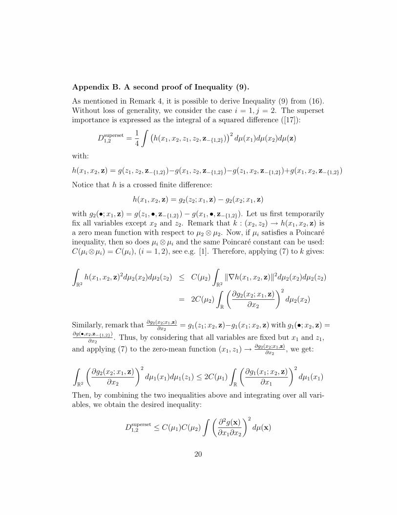
Appendix B. A second proof of Inequality (9).

As mentioned in Remark 4, it is possible to derive Inequality (9) from (16).Without loss of generality, we consider the case i = 1, j = 2. The supersetimportance is expressed as the integral of a squared difference ([17]):

Dsuperset1,2 =

1

4

∫ (h(x1, x2, z1, z2, z−{1,2})

)2dµ(x1)dµ(x2)dµ(z)

with:

h(x1, x2, z) = g(z1, z2, z−{1,2})−g(x1, z2, z−{1,2})−g(z1, x2, z−{1,2})+g(x1, x2, z−{1,2})

Notice that h is a crossed finite difference:

h(x1, x2, z) = g2(z2; x1, z) − g2(x2; x1, z)

with g2(•; x1, z) = g(z1, •, z−{1,2}) − g(x1, •, z−{1,2}). Let us first temporarilyfix all variables except x2 and z2. Remark that k : (x2, z2) → h(x1, x2, z) isa zero mean function with respect to µ2 ⊗ µ2. Now, if µi satisfies a Poincareinequality, then so does µi ⊗µi and the same Poincare constant can be used:C(µi⊗µi) = C(µi), (i = 1, 2), see e.g. [1]. Therefore, applying (7) to k gives:

∫

R2

h(x1, x2, z)2dµ2(x2)dµ2(z2) ≤ C(µ2)

∫

R2

‖∇h(x1, x2, z)‖2dµ2(x2)dµ2(z2)

= 2C(µ2)

∫

R

(∂g2(x2; x1, z)

∂x2

)2

dµ2(x2)

Similarly, remark that ∂g2(x2;x1,z)∂x2

= g1(z1; x2, z)−g1(x1; x2, z) with g1(•; x2, z) =∂g(•,x2,z−{1,2})

∂x2. Thus, by considering that all variables are fixed but x1 and z1,

and applying (7) to the zero-mean function (x1, z1) → ∂g2(x2;x1,z)∂x2

, we get:

∫

R2

(∂g2(x2; x1, z)

∂x2

)2

dµ1(x1)dµ1(z1) ≤ 2C(µ1)

∫

R

(∂g1(x1; x2, z)

∂x1

)2

dµ1(x1)

Then, by combining the two inequalities above and integrating over all vari-ables, we obtain the desired inequality:

Dsuperset1,2 ≤ C(µ1)C(µ2)

∫ (∂2g(x)

∂x1∂x2

)2

dµ(x)

20

References

[1] C. Ane, S. Blachere, D. Chafaı, P. Fougeres, I. Gentil, F. Malrieu,C. Roberto, G. Scheffer, Sur les inegalites de Sobolev logarithmiques,volume 10 of Panoramas et Syntheses, Societe Mathematique de France,Paris, 2000.

[2] M. Bagnoli, T. Bergstrom, Log-concave probability and its applications,Economic Theory 26 (2005) 445–469.

[3] S.G. Bobkov, Isoperimetric and analytic inequalities for log-concaveprobability measures, The Annals of Probability 27 (1999) 1903–1921.

[4] S.G. Bobkov, C. Houdre, Isoperimetric constants for product probabilitymeasures, The Annals of Probability 25 (1997) 184–205.

[5] D. Cacuci, Sensitivity and uncertainty analysis - Theory, Chapman &Hall/CRC, Paris, 2003.

[6] B. Efron, C. Stein, The jackknife estimate of variance, The Annals ofStatistics 9 (1981) 586–596.

[7] J. Friedman, B. Popescu, Predictive Learning via Rule Ensembles, TheAnnals of Applied Statistics 2 (2008) 916–954.

[8] J. Fruth, O. Roustant, S. Kuhnt, Total interaction index: A variance-based sensitivity index for interaction screening, Journal of StatisticalPlanning and Inference 147 (2014) 212–223.

[9] A. Griewank, G. Corliss, Automatic differentiation of algorithms: The-ory, implementation and application, SIAM, Philadelphia, 1991.

[10] W. Hoeffding, A class of statistics with asymptotically normal distribu-tions, Annals of Mathematical Statistics 19 (1948) 293–325.

[11] T. Homma, A. Saltelli, Importance measures in global sensitivity anal-ysis of nonlinear models, Reliability Engineering & System Safety 52(1996) 1–17.

[12] G. Hooker, Discovering additive structure in black box functions, in:Proceedings of KDD 2004, ACM DL, pp. 575–580.

21

[13] B. Iooss, A.L. Popelin, G. Blatman, C. Ciric, F. Gamboa, S. Lacaze,M. Lamboni, Some new insights in derivative-based global sensitivitymeasures, in: Proceedings of PSAM 11 & ESREL 2012 Conference,Helsinki, Finland, pp. 1094–1104.

[14] M. Jansen, Analysis of variance designs for model output, ComputerPhysics Communication 117 (1999) 25–43.

[15] S. Kucherenko, M. Rodriguez-Fernandez, C. Pantelides, N. Shah, Montecarlo evaluation of derivative-based global sensitivity measures, Relia-bility Engineering and System Safety 94 (2009) 1135–1148.

[16] M. Lamboni, B. Iooss, A.L. Popelin, F. Gamboa, Derivative-based globalsensitivity measures: General links with Sobol’ indices and numericaltests, Mathematics and Computers in Simulation 87 (2013) 45–54.

[17] R. Liu, A. Owen, Estimating mean dimensionality of analysis of vari-ance decompositions, Journal of the American Statistical Association101 (2006) 712–721.

[18] A. Marrel, B. Iooss, B. Laurent, O. Roustant, Calculations of the Sobolindices for the Gaussian process metamodel, Reliability Engineering andSystem Safety 94 (2009) 742–751.

[19] T. Muehlenstaedt, O. Roustant, L. Carraro, S. Kuhnt, Data-driven Krig-ing models based on FANOVA-decomposition, Statistics & Computing22 (2012) 723–738.

[20] A. Prekopa, Logarithmic concave measures with applications to stochas-tic programming, Acta Scientiarium Mathematicarum 32 (1971) 301–316.

[21] M. Rodriguez-Fernandez, J. Banga, F. Doyle, Novel global sensitivityanalysis methodology accounting for the crucial role of the distributionof input parameters: application to systems biology models, Interna-tional Journal of Robust Nonlinear Control 22 (2012) 1082–1102.

[22] A. Saltelli, K. Chan, E. Scott, Sensitivity analysis, Wiley series in prob-ability and statistics, Wiley, Chichester, 2000.

22

[23] A. Saltelli, M. Ratto, T. Andres, F. Campolongo, J. Cariboni, D. Gatelli,M. Saisana, S. Tarantola, Global Sensitivity Analysis: The Primer,Wiley-Interscience, 2008.

[24] I. Sobol, Sensitivity estimates for non linear mathematical models,Mathematical Modelling and Computational Experiments 1 (1993) 407–414.

[25] I. Sobol, Theorems and examples on high dimensional model represen-tation, Reliability Engineering and System Safety 79 (2003) 187–193.

[26] I. Sobol, A. Gershman, On an alternative global sensitivity estimator,in: Proceedings of SAMO 1995, Belgirate, Italy, pp. 40–42.

[27] I. Sobol, S. Kucherenko, Derivative-based global sensitivity measuresand the link with global sensitivity indices, Mathematics and Computersin Simulation 79 (2009) 3009–3017.

[28] I. Sobol, S. Kucherenko, A new derivative based importance criterionfor groups of variables and its link with the global sensitivity indices,Computer Physics Communications 181 (2010) 1212–1217.

[29] C. Storlie, J. Helton, Multiple predictor smoothing methods for sensi-tivity analysis: Description of techniques, Reliability Engineering andSystem Safety 93 (2008) 28–54.

23