crowd location forecasting at points of interest jorge...

Crowd Location Forecasting at Points of Interest

Jorge Alvarez-Lozano

Computer Science Department,CICESE Research CenterCarr. Ensenada-Tijuana 3918Ensenada, MexicoE-mail: [email protected]

J. Antonio Garcıa-Macıas*Computer Science Department,CICESE Research CenterCarr. Ensenada-Tijuana 3918Ensenada, MexicoE-mail: [email protected]*Corresponding author

Edgar Chavez

Institute of Mathematics, UNAMMexicoE-mail: [email protected]

Abstract: Predicting the location of a mobile user in the near future can be used for alarge number of user-centered ubiquitous applications. This can be extended to crowd-centered applications if a large number of users is included. In this paper we present aspatio-temporal prediction approach to forecast user location in a medium-term period.Our approach is based on the hypothesis that users exhibit a different mobility patternfor each day of the week. Once factored out this weekly pattern, user mobility amongpoints of interest is postulated to be markovian.

We trained a hidden Markov model to forecast user mobility and evaluated ourapproach using a public dataset. The experimental results show that our approach iseffective considering a time period of up to seven hours. We obtained an accuracy of upto 81.75 % for a period of 30 minutes, and 66.25 % considering 7 hours.

Keywords: Data mining; Data sharing; Spatio-temporal crowd location forecasting; Userlocation predictability; User mobility similarity.

Reference to this paper should be made as follows: Alvarez-Lozano, J., Garcıa-Macıas,J. A. and Chavez, E. (2013) ‘Crowd Location Forecasting at Points of Interest’, Int. J.Ad Hoc and Ubiquitous Computing, Vol. x, No. x, pp.xxx–xxx.

Biographical notes: Jorge Alvarez-Lozano is a PhD student in the Computer ScienceDepartment at CICESE Research Center, Ensenada, Baja California, Mexico. Hisresearch interests include participatory sensing, opportunistic communications, datamining, location-based services, and social networking. Alvarez-Lozano received an MScin Computer Science from CICESE.

J. Antonio Garcıa-Macıas is a researcher in the Computer Science Department at CICESEResearch Center, Ensenada, Baja California, Mexico. His research interests includeubiquitous computing, human-computer interaction, and computer networks. He receiveda PhD in Computer Science from Institut National Polytechnique de Grenoble, France.

Edgar Chavez. He received the B.S. degree in Mathematics from the UniversidadMichoacana de San Nicolas de Hidalgo, a M.S. degree in Computer Science from theUniversidad Nacional Autonoma de Mexico, and a PhD in Computer Science fromthe Centro de Investigacion en Matematicas, Mexico. He is currently a full professorin Universidad Nacional Autonoma de Mexico. He has chaired major conferences incomputer science, has been president of the Mexican Computer Science Society, andhave published over 100 technical contributions in different venues. His research interestsinclude storage, retrieval, analysis and mining of data.

Int. J.of Ad Hoc and Ubiquitous Computing, Vol. x, No. x, 2013 2

1 Introduction

The ability to forecast user location in an accurate wayis central to many research areas such as urban planning,healthcare, pervasive and ubiquitous systems, computernetworks and recommender systems, to name a few.With the increasing proliferation of mobile devices andthe huge variety of sensors incorporated on them, itis possible to register the user location on the moveand hence mobile devices become a very rich source ofcontextual data. We are interested in predicting userlocation based on her past history, in particular we areinterested in knowing if a given user will be at a pointof interest at a given time. User mobility patterns havebeen studied, and researchers have found that peopleexhibit a high degree of repetition, visiting regular placesduring their daily activities (Gonzalez et al. (2008)). Thisregularity of the past movements has been exploited toforecast the next location of the user. This approach hasbeen useful for domains where the time lapse betweenlocations is not relevant; a more complex scenario requirealso to know when the user will be at the given location.The former problem has been analyzed in Scellato et al.(2011) and Sadilek & Krumm (2012), they are ableto predict the user location in space and time (a.k.a.spatio-temporal prediction) for short and long-term timelapses respectively. We are interested in a more preciseforecasting of the user location, lets see the scenario.Assume current time is 10:00 AM (T ), what we want toknow is: Where a user will be in the next 3 to 5 hours([T, T + ∆(T )] for some ∆(T )). We have not found inthe literature a solution for this medium-term spatio-temporal prediction.

After mining individual mobility patterns, we are ableto join the individual predictions, and to serve unspecificapplications for the crowd. The general public (includingbanks, retail stores or traffic authorities) could querya location forecasting service to know the capacity ofa specific Point of Interest (POI). In one applicationscenario, a user may query the capacity of a givenPOI (think for example in a fast food location) anddecide between many different alternatives based on thatmeasure.

A more specialized service can warn the user abouta potential overcrowded POI she is about to visit in thenext few hours. This is a potential paradox, since allusers using the service may back-off and avoid the POI,which will not be overcrowded at the end. This mayhave the same effect of trying to predict the behaviorof individual stock options. Any successful forecastingalgorithm can change the behavior of a system. For thetime being we will focus on forecasting the user locationwithout worrying about paradoxical behavior.

Users should be assured about the potential usage oftheir data. Disclosing their current location implies theyare disclosing travel patterns and the individual forecastof their location. The service should provide secure waysto disclose the location of anonymous users, since the

Copyright c© 2008 Inderscience Enterprises Ltd.

objective is to infer the location of a crowd in a givenPOI.

In this work, we present a medium-term spatio-temporal prediction model based on the repetitivepatterns of people visiting some specific places that areimportant for them. We found that the user mobilityamong the POIs can be modeled as a Markovian chain.Then, considering the Markovian property among POIs,and the relation of staying time with specific timeperiods, we modeled the mobility as a hidden MarkovModel (HMM).

The proposed approach to forecast the crowd locationconsists of two steps. First, for each user we identifythe current significant places or points of interest. Then,using the records of the visits to the significant places,we define the user mobility as an HMM, with whichwe are able to predict where a user will be in a giventime period. The contribution of this paper can besummarized as follows:

• We identified the minimum time period coveringthe current mobility pattern of a user. Wecompared the daily user mobility using the cosinesimilarity and as a result, we identified currentpoints of interest. This enabled an accurateprediction model.

• We present a method to forecast the user locationusing a hidden Markov model. Our approachpostulate, and experimentally prove, a markovianproperty found in the user mobility among POIs.

• We used the public GeoLife GPS trajectory dataset(Zheng et al. (2008, 2009, 2010)) to evaluate ourapproach.

• We compared our approach with a method basedon NextPlace (Scellato et al. (2011)). With ourmethod, we report an overall prediction accuracyof up to 85 % for short prediction periods, withan accuracy of up to 70 % when the predictionperiod is 7 hours, both higher than the baseline ofNextPlace.

The rest of this paper is organized as follows:we start discussing some of the work related tospatial and spatio-temporal forecasting, and discussthe characteristics of the mobility defining the spatio-temporal prediction model. Later we present amethodology to define the spatio-temporal prediction,introducing some application scenarios, and proceedwith an experimental evaluation using a public dataset. Finally, we discuss the scope and limitation of ourapproach and give some conclusions.

2 Related work

Most of the current methods for mining and forecastinguser location are oriented to a single user instead ofa crowd. In applications where a crowd is going to be

Copyright c© 2009 Inderscience Enterprises Ltd.

Crowd Location Forecasting at Points of Interest 3

tracked at once the method should scale. We believe thatusing an automata for each user to predict her position isan scalable way to implement crowd forecasting becausethe automata related to an user can be queried inconstant time. This is the motivation of our work andour solution approach.

Mobility prediction, mobility mining or mobilityforecasting have many different sources depending on theapplication. Some authors try to characterize activitiesand traveling paths to obtain behavior patterns andto predict user mobility (Ashbrook & Starner (2003),Chon et al. (2012), Eagle & Pentland (2006), Kim et al.(2006), Sadilek & Krumm (2012), Ye et al. (2009),Yuan et al. (2011), Zheng et al. (2008), Zheng & Xie(2010)). According to our approach, we can distinguishthe related work as spatial prediction and spatio-temporalprediction.

The goal of the spatial prediction is to identify thenext place or places where the user will be. Some existingapproaches are able to forecast just the next location of auser, but not the time when the user will be at the place(Ashbrook & Starner (2003), Kim et al. (2006), Krumm& Horvitz (2006), Liao et al. (2006), Nicholson & Noble(2008), Song et al. (2006)). Krumm & Horvitz (2006)present a method to forecast the driver’s destinationusing GPS trajectories as the journey progresses andthe driver moves from a geographical region to another.A similar approach is presented in Yavas et al. (2004)where the objective is to predict in which cell of acellular network the user will be, being the restrictionthe topology, there are only a limited number of cellsthe user can reach from the current location. Anotherwork is BreadCrumbs (Nicholson & Noble (2008)), theauthors use discrete data to estimate the next userlocation providing network connectivity. In WhereNext(Monreale et al. (2009)), the authors use previoustrajectory patterns (sequences of regions), which aremodeled as a tree. Later, considering a new trajectorythe next location is predicted finding the most likelysequence path in the tree. Using the above approaches,predictions cannot be extended into the future becausethey are just focused on the next place to be visited.These previous works are based on markovian orbayesian models. A more recent work uses HMMs, andthe same dataset we use to forecast the user location.However, they define on a different way the HMM; theyare interested in the mobility among geographical regionsinstead of points of interest (Mathew et al. (2012)). Anevaluation of several techniques to forecast the next userlocation can be found in Song et al. (2003).

Regarding to spatio-temporal prediction, in Vu et al.(2011) traces of Wi-Fi and Bluetooth (the user log toa place) are used to find regular patterns in order topredict where a user will be at a given time, how long theuser will stay at that place, and also infer who the userwill meet there. To do the spatio-temporal prediction,traces are split according to different time periods. Then,for a given period the most likely location is returned.Meanwhile, Krumm & Brush (2011) present a method

to predict when a user will be at home or away, based onprevious observations of presence there. One particularapproach is NextPlace (Scellato et al. (2011)), which isgeneral enough to be significant to compare with ourapproach. The authors get as reference the sequenceof the current places visited by a user, and using thehistorical records search for a similar pattern in the pastto predict the next place the user will visit and the timeshe will stay there. In Scellato et al. (2011), the bestaccuracy (about 90 %) is obtained when the predictionperiod (∆(T )) is only about 5 minutes, if the predictionperiod increases to 60 minutes the accuracy drops to 70%. Although the above works have been useful in somedomains, they do not offer the functionality required todo the medium-term spatio-temporal prediction. Also,they do not consider just the current mobility pattern,neither they distinguish a particular pattern for each dayof the week. Finally, they do not consider the transitionamong significant places.

3 User mobility

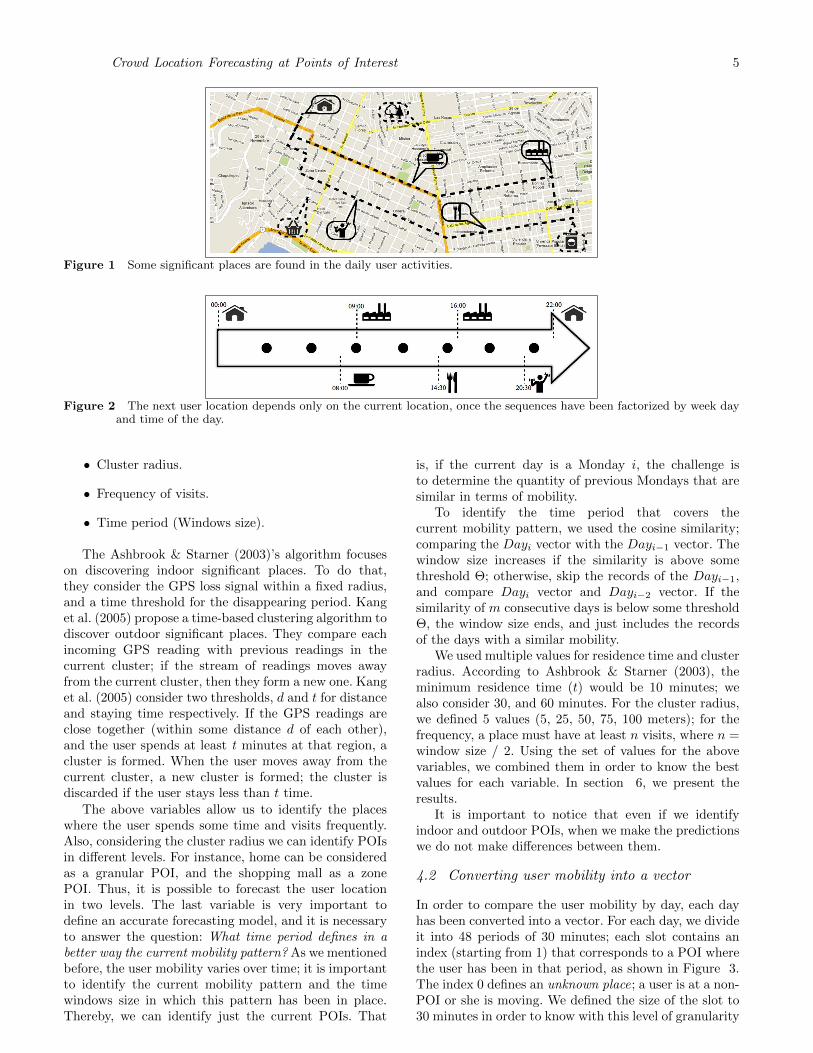
Although user mobility seems to be dynamic, mostpeople follow certain mobility patterns (Eagle &Pentland (2006), Farrahi & Gatica-Perez (2011),Gonzalez et al. (2008)); it is rare to have a completelyerratic behavior over time. Mobility is fixed by ouractivities and habits, like working, school attendance,recreational endeavors, and other activities that varyover time within certain behavior boundaries. We candistinguish between weekday, weekend, monthly orannually patterns. This is analyzed in Eagle & Pentland(2006), Motahari et al. (2012), Yavas et al. (2004). Oncerecognized the user mobility patterns, we are able topredict her spatio-temporal location. In this work wefixed our attention in three major categories of usermobility and with their interrelation we can infer theuser mobility in general, Figure 2 illustrates.

3.1 Temporal patterns

It is reasonable to assume certain periodicity inlocation/time patterns. Usually weekdays are similar,people tend to organize their life according to workor school hours, and our hypothesis is that activitiesin the same weekday will have a repetitive pattern. Acorresponding periodicity is observed during weekends.Mobility exhibits a different pattern for each day of theweek (Chon et al. (2012), Farrahi & Gatica-Perez (2011),Hsu et al. (2007), Motahari et al. (2012)). Hence, theplaces visited in a given day are postulated to be thesame for the subsequent days.

Two additional observations are that the currentlocation in a given day and hour conditions the nextplace to be visited. For example if one user is at homeat 7:00 AM on a Monday, the next place he will beat is most likely the coffee shop or the office, but notthe restaurant or a movie theater. We postulate the

4 J. Alvarez-Lozano, J. A. Garcıa-Macıas and E. Chavez

user mobility is a markovian stochastic process andcan be described with a Markov Chain. The Markovianproperty (Markov (1961)) would state that current placeis only a function of the previous place. Our main claimis that once the data is grouped by day and time, thesequence of places visited form a Markovian chain.

3.2 Markovian chain among POIs

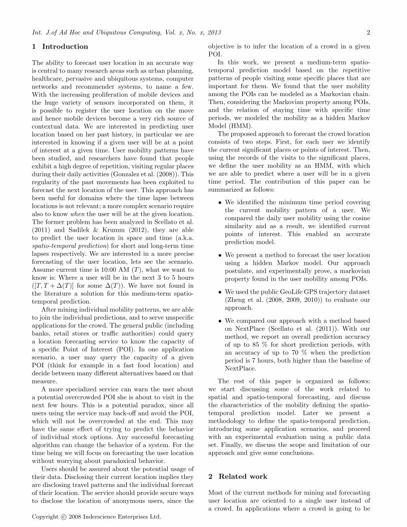
Considering our above claim, it is necessary to clarifythat the markovian property is just valid when theuser moves among certain discrete places. These discretelocations are distinguished because the user spendssome time and visit them frequently; they are knownas significant places or points of interest (POI). Forinstance, considering the user mobility on a givenMonday, after he is at home, he goes to the coffee shop,then to a super market, then to his work. After somehours, he goes to the restaurant, returns to his work,then he goes to the gym, and finally he goes back home.Next Monday, his mobility does not differ too much,after leaving home, he goes to the coffee shop, thento the laundry, and work. Around 2:00 PM, he goesto the restaurant, returns to his work, then he goes tothe gym, and finally he goes back to home. Consideringthis scenario, it is possible to identify places that arePOIs (Figure 1 black shape), and those which visitoccasionally (Figure 1 dotted line). Also, we can observethat the mobility among POIs does not change (home,coffee shop, work, restaurant, work, gym, home); just theplaces visited in the transition between POIs change. Werefer the reader to the Figure 1.

3.3 Modeling user mobility as a hidden Markovmodel

Using the above hypothesis, it is possible to modelthe user mobility as an HMM (Rabiner (1989)) (SeeFigure 5). A hidden Markov model is a finite statemachine consisting of a set of hidden states (Q), aset of observations (O), transition probabilities (A),emission probabilities (B), and initial probabilities foreach state (π). Hidden states are not directly visible,while observations (dependents on the state) are visible.Each state has a probability distribution over the setof observations (λ = (A,B, π)). In our case, the hiddenstates corresponds to POIs, which have a probabilitydistribution over times of day. Once the HMM hasbeen defined, three inference problems can be addressed,(i) finding the probability of an observed sequence(evaluation); (ii) finding the sequence of hidden statesthat most probably generated an observed sequence(decoding); (iii) generating an HMM given a sequence ofobservations (learning). For the purpose of this work, weuse the decoding approach; given a time period (sequenceof observations), we want to know the most likelysequence of locations where the user will be (hiddenstates). More detail can be found in section 4.5.

4 Methodology

To address the challenge of forecasting user mobility inspace and time, we first convert the GPS readings intoindoor and outdoor POIs. Then, using the records of thevisits to the identified POIs, an HMM is defined for eachday and for each user. Once, the HMM is defined, wemake some predictions.

4.1 Identifying points of interest

Discovering significant places for an user has been animportant research topic in several applications suchas ambient assisted living, ubiquitous computing, andothers. Mobile traces produced by the mobile devices,provide a great amount of location data useful todiscover where the user spends her time. Thereby,with this amount of location data there is a need foralgorithms that deal with the challenge of turning datainto significant places (Ashbrook & Starner (2003), Kanget al. (2005), Kim et al. (2006), Marmasse & Schmandt(2000), Palma et al. (2008), Ram et al. (2010), Zhenget al. (2009), Zhou et al. (2007)). At the moment, someworks have been focused on discovering these placesusing different approaches, and for different purposes.These can be classified as follows:

• Residence time-based algorithms. This approach isbased on the assumption that the importance of aplace is directly proportional to the permanence atit (Kang et al. (2005), Kim et al. (2006), Scellatoet al. (2011), Ye et al. (2009)).

• Density-based clustering algorithms. These arebased on the density of GPS points (Ram et al.(2010), Zhou et al. (2007)).

• Lost signal-based algorithms. This approach hasbeen used to discover indoor POIs, using the GPSsignal disappearance and reappearance (Ashbrook& Starner (2003), Marmasse & Schmandt (2000)).

The intuition behind the first two approaches offersa good functionality for some specific applications,nonetheless, for our approach they have a limitation.It is not possible to take into account just one ofthose, because maybe a given user was at a place fora long time, but that happened some months ago; or,considering the density-based algorithms, a place canbe considered significant after taking into account theGPS points of several visits. Thereby, it is necessary toconsider time and location data, as well the frequencyof visits and the time period that covers the currentmobility pattern. This way, we are enabled to identifythe places that are currently significant, and therefore,define in a better way the forecasting model.

In order to identify indoor and outdoor POIs, we haveapplied the below criterions to the algorithms of previousworks (Ashbrook & Starner (2003), Kang et al. (2005)).

• Residence time.


Figure 1 Some significant places are found in the daily user activities.

Figure 2 The next user location depends only on the current location, once the sequences have been factorized by week dayand time of the day.

• Cluster radius.

• Frequency of visits.

• Time period (Windows size).

The Ashbrook & Starner (2003)’s algorithm focuseson discovering indoor significant places. To do that,they consider the GPS loss signal within a fixed radius,and a time threshold for the disappearing period. Kanget al. (2005) propose a time-based clustering algorithm todiscover outdoor significant places. They compare eachincoming GPS reading with previous readings in thecurrent cluster; if the stream of readings moves awayfrom the current cluster, then they form a new one. Kanget al. (2005) consider two thresholds, d and t for distanceand staying time respectively. If the GPS readings areclose together (within some distance d of each other),and the user spends at least t minutes at that region, acluster is formed. When the user moves away from thecurrent cluster, a new cluster is formed; the cluster isdiscarded if the user stays less than t time.

The above variables allow us to identify the placeswhere the user spends some time and visits frequently.Also, considering the cluster radius we can identify POIsin different levels. For instance, home can be consideredas a granular POI, and the shopping mall as a zonePOI. Thus, it is possible to forecast the user locationin two levels. The last variable is very important todefine an accurate forecasting model, and it is necessaryto answer the question: What time period defines in abetter way the current mobility pattern? As we mentionedbefore, the user mobility varies over time; it is importantto identify the current mobility pattern and the timewindows size in which this pattern has been in place.Thereby, we can identify just the current POIs. That

is, if the current day is a Monday i, the challenge isto determine the quantity of previous Mondays that aresimilar in terms of mobility.

To identify the time period that covers thecurrent mobility pattern, we used the cosine similarity;comparing the Dayi vector with the Dayi−1 vector. Thewindow size increases if the similarity is above somethreshold Θ; otherwise, skip the records of the Dayi−1,and compare Dayi vector and Dayi−2 vector. If thesimilarity of m consecutive days is below some thresholdΘ, the window size ends, and just includes the recordsof the days with a similar mobility.

We used multiple values for residence time and clusterradius. According to Ashbrook & Starner (2003), theminimum residence time (t) would be 10 minutes; wealso consider 30, and 60 minutes. For the cluster radius,we defined 5 values (5, 25, 50, 75, 100 meters); for thefrequency, a place must have at least n visits, where n =window size / 2. Using the set of values for the abovevariables, we combined them in order to know the bestvalues for each variable. In section 6, we present theresults.

It is important to notice that even if we identifyindoor and outdoor POIs, when we make the predictionswe do not make differences between them.

4.2 Converting user mobility into a vector

In order to compare the user mobility by day, each dayhas been converted into a vector. For each day, we divideit into 48 periods of 30 minutes; each slot contains anindex (starting from 1) that corresponds to a POI wherethe user has been in that period, as shown in Figure 3.The index 0 defines an unknown place; a user is at a non-POI or she is moving. We defined the size of the slot to30 minutes in order to know with this level of granularity


where the user has been; we also considered slots of 15and 60 minutes; however, there is no significant differenceconsidering a slot size of 15 minutes. In contrast, using aslot of 60 minutes we obtained a lower similarity; it wasmore likely to find some POIs in a same slot.

4.3 Updating POIs

As mentioned before, the user activities vary over time,and therefore his mobility. Consider for example that agiven user is starting swimming classes on Monday, from7:30 AM to 8:30 AM at a public pool (Top of Figure 4,block D). For the subsequent Mondays, the user takeshis classes at the same time; however, the public poolis not a POI yet because it does not have the numberof visits required (the relative frequency is small). Someweeks after, the public pool has the required visits to bea POI; the HMM is updated (Bottom of Figure 4). TheHMM also is updated when a place ceases to be a POI.For instance, when the mentioned user no longer takeshis swimming classes. As Ashbrook & Starner (2003)mentioned, a limitation of using the Markov approachis that a behavior change may take a long time to bereflected. To address this challenge, we propose to updateday after day the POIs and the information related tothem (Figure 4). A feasible option would be that the userexplicitly specifies his behavior change, or that the userselects from a set of recognized patterns, the appropriateone according to the season.

4.4 Defining user prediction model

The HMM is defined as follows:

• Hidden states. These are defined by the POIs. Also,another hidden state was added to define when theuser is at a location that is not a POI.

• Observations. These are defined by the averageof the arrival and leaving time to the POIs.According to Do & Gatica-Perez (2012), the arrivaland leaving times to some places do not changemuch; for instance, considering the work or scholaractivities, there are times defined for arrival andleaving. This way, we can define in an accurate waythe time when the user will be at a POI; otherwise,considering the leaving time, we can define that heis at another POI, or at a non POI.

• Vector π. It defines the probability that the userstarts his day at a given POI.

• Transition matrix. It defines the probability thatthe user moves from a POI to another, or from aPOI to the state that corresponds to a non-POI.

• Confusion matrix. It defines the probability thatthe user is at a given POI (or at a non-POI), at agiven time.

Once the HMM is defined, we are able to forecast theuser location in a given time period (See Figure 5). Forinstance, if the current time is 11:00 AM, and we wantto know where the user will be in the period 11:00 -18:00, the vector π, transition matrix (A), and confusionmatrix (B), are used to identify the combinations ofhidden states (and their corresponding probabilities)that satisfy such time period, so later the sequence ofhidden states with the highest probability can be selected(decoding problem). In order to identify the sequence ofhidden states with the highest probability, we used theViterbi algorithm (Viterbi (2006)).

4.5 Viterbi’s algorithm

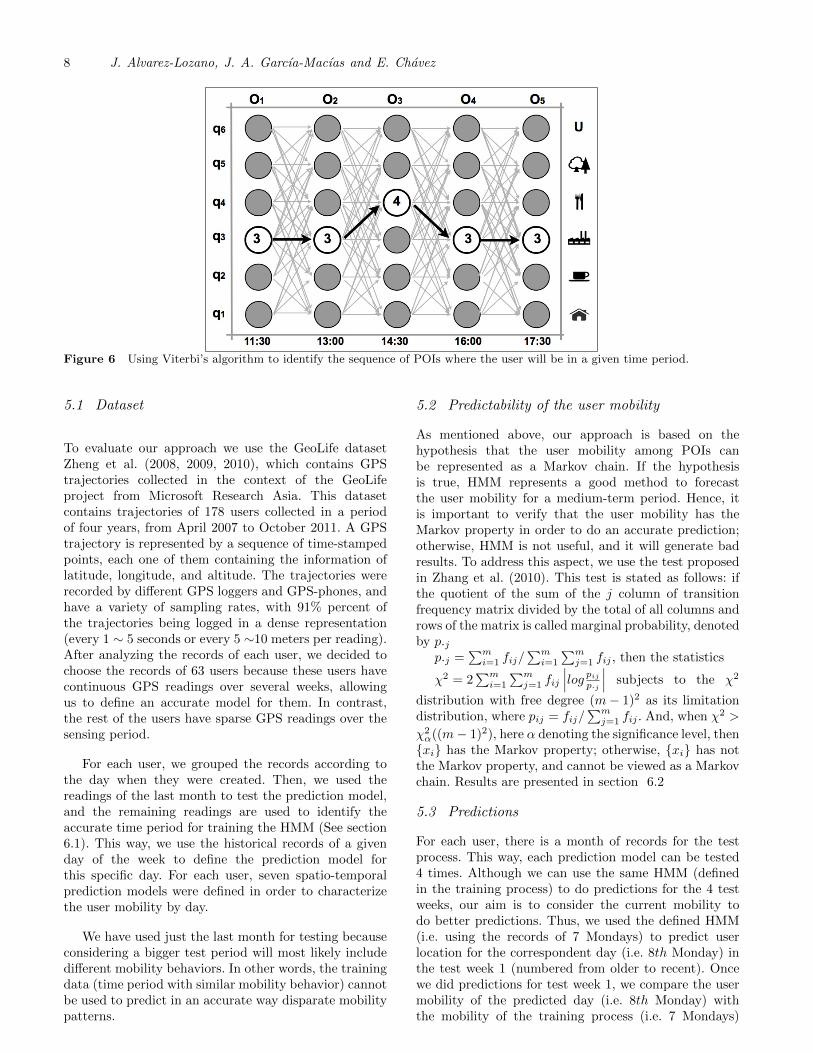
As mentioned on section 3.3, the aim of the decodingproblem is to discover the hidden state sequence thatwas most likely to have produced a given observationsequence. One solution is to use Viterbi’s algorithm tofind the single best state sequence for an observationsequence. Viterbi’s algorithm is a trellis algorithmthat is very similar to the forward algorithm usedin the evaluation problem, except that the transitionprobabilities are maximized at each step, instead ofadded (See Figure 6). Viterbi’s algorithm is as follows,first it defines:

δt(i) = maxqi,q2,...,qt−1P (qiq2...qt = si, oi, o2...ot|λ) (1)

as the probability of the most probable state path forthe partial observation sequence. Then:

Initialization:

δ1(i) = πibi(o1), 1 ≤ i ≤ N,ψ1(i) = 0 (2)

Recursion:

δts(i) = max1≤i≤N [δt−1(i)aij ] bj(ot),

2 ≤ t ≤ T, 1 ≤ j ≤ N (3)

ψt(j) = argmax1≤i≤N [δt−1(i)aij ] ,

2 ≤ t ≤ T, 1 ≤ j ≤ N (4)

Termination:

P ∗ = max1≤i≤N [δT (i))] (5)

q∗T = argmax1≤i≤N [δT (i))] (6)

Optimal state sequence backtracking:

q∗T = ψt+1q∗T+1, t = T − 1, T − 2, ...., 1 (7)

5 Evaluation

To test the efficacy of our spatio-temporal prediction,we compared our approach against a modified versionof NextPlace (hereby defined as NP*). To the best ofour knowledge, NextPlace’s results have been the best


Figure 3 User mobility as a vector.

Figure 4 The update process of POIs is made for each day of the week (e.g. Monday) considering the user mobility weekover week

Figure 5 An HMM representing some POIs and their relationship with different hours of the day.

in the literature. NextPlace includes two methods: oneto predict the user location at a given time, and anotherto predict the residence time at that place. The NP*method just includes the method to forecast the userlocation at a given time; POI selection remains the same.Our method estimates the full sequence of POIs wherethe user will be in a given time period, while NP*estimates the place where the user will be at a specifictime. For this reason, and to do a fair comparison of theperformance of both methods, for each observation inthe time period we apply the NP* method using the best

value for m (m = 3, more detail about the variable mcan be found in Scellato et al. (2011)) to predict wherethe user will be. That is, if we want to know the sequenceof POIs in the [11 : 00, 15 : 00] period, and consideringthat for this period there are 3 observations defined (e.g.11:30, 13:00,14:30), we apply the NP* method for eachone of these observations. Then, we average the resultsin order to compare them with our method.


Figure 6 Using Viterbi’s algorithm to identify the sequence of POIs where the user will be in a given time period.

5.1 Dataset

To evaluate our approach we use the GeoLife datasetZheng et al. (2008, 2009, 2010), which contains GPStrajectories collected in the context of the GeoLifeproject from Microsoft Research Asia. This datasetcontains trajectories of 178 users collected in a periodof four years, from April 2007 to October 2011. A GPStrajectory is represented by a sequence of time-stampedpoints, each one of them containing the information oflatitude, longitude, and altitude. The trajectories wererecorded by different GPS loggers and GPS-phones, andhave a variety of sampling rates, with 91% percent ofthe trajectories being logged in a dense representation(every 1 ∼ 5 seconds or every 5 ∼10 meters per reading).After analyzing the records of each user, we decided tochoose the records of 63 users because these users havecontinuous GPS readings over several weeks, allowingus to define an accurate model for them. In contrast,the rest of the users have sparse GPS readings over thesensing period.

For each user, we grouped the records according tothe day when they were created. Then, we used thereadings of the last month to test the prediction model,and the remaining readings are used to identify theaccurate time period for training the HMM (See section6.1). This way, we use the historical records of a givenday of the week to define the prediction model forthis specific day. For each user, seven spatio-temporalprediction models were defined in order to characterizethe user mobility by day.

We have used just the last month for testing becauseconsidering a bigger test period will most likely includedifferent mobility behaviors. In other words, the trainingdata (time period with similar mobility behavior) cannotbe used to predict in an accurate way disparate mobilitypatterns.

5.2 Predictability of the user mobility

As mentioned above, our approach is based on thehypothesis that the user mobility among POIs canbe represented as a Markov chain. If the hypothesisis true, HMM represents a good method to forecastthe user mobility for a medium-term period. Hence, itis important to verify that the user mobility has theMarkov property in order to do an accurate prediction;otherwise, HMM is not useful, and it will generate badresults. To address this aspect, we use the test proposedin Zhang et al. (2010). This test is stated as follows: ifthe quotient of the sum of the j column of transitionfrequency matrix divided by the total of all columns androws of the matrix is called marginal probability, denotedby p.j

p.j =∑mi=1 fij/

∑mi=1

∑mj=1 fij , then the statistics

χ2 = 2∑mi=1

∑mj=1 fij

∣∣∣log pijp.j ∣∣∣ subjects to the χ2

distribution with free degree (m− 1)2 as its limitationdistribution, where pij = fij/

∑mj=1 fij . And, when χ2 >

χ2α((m− 1)2), here α denoting the significance level, then{xi} has the Markov property; otherwise, {xi} has notthe Markov property, and cannot be viewed as a Markovchain. Results are presented in section 6.2

5.3 Predictions

For each user, there is a month of records for the testprocess. This way, each prediction model can be tested4 times. Although we can use the same HMM (definedin the training process) to do predictions for the 4 testweeks, our aim is to consider the current mobility todo better predictions. Thus, we used the defined HMM(i.e. using the records of 7 Mondays) to predict userlocation for the correspondent day (i.e. 8th Monday) inthe test week 1 (numbered from older to recent). Oncewe did predictions for test week 1, we compare the usermobility of the predicted day (i.e. 8th Monday) withthe mobility of the training process (i.e. 7 Mondays)


using the cosine similarity. If the similarity is above somethreshold Θ (Θ = 0.50), the current HMM is updatedwith the records of the predicted day. Otherwise, thecurrent HMM is used to predict the user location for thetest week 2 (i.e. 9th Monday). This process is appliedfor the subsequent weeks 3 and 4 (i.e. 10th and 11thMonday)

For each spatio-temporal prediction model, we havemade five predictions considering different values for∆T (30 minutes, 1, 3, 5, and 7 hours). A total of 140predictions for each user, 35 for each test week. Eachprediction is uniformly distributed over the [00:00,17:00]interval. We selected this interval because if T = 17 :00, it is possible to know in which POIs a user will beusing the largest value for ∆T (7 hours). In total, 8820predictions were made using 1st order HMM.

5.4 Effectiveness of the prediction model

To determine the effectiveness of the prediction, if weestimate where a user will be in the interval [T, T + ∆T ],the prediction is correct if the user is at place qi inthe interval [Tpred − θ, Tpred + θ] , θ represents an errormargin. That is, a prediction is correct when the user isat the POI defined by qi, at the time indicated by theobservation oi with certain error margin. It would alsobe correct if the prediction indicates that the user is notat a POI (in the case of the state corresponding to anunknown place). We have defined θ = 15 minutes.

Tpred = T + oi 1 ≤ i ≤ No. of obs. in the interval (8)

6 Results

6.1 POIs

To define an accurate prediction model, we identifiedthe time period that comprises the current mobilitypattern. Thus, for each user, and for each day of theweek, we identify this period. On average the time period(windows size) is about 7.3 weeks, the shorter timeperiod is 4 weeks, and the longer is 11 weeks; the timeperiod is used for training each HMM.

We want to find the values of minimum residencetime and cluster radius maximizing POI identification.Figure 7 show the amount of time the users spend atPOIs considering 3 values for residence time (10, 30, and60 minutes ), and five values for the cluster radius (5, 25,50, 75, 100 meters). As it can be seen in Figure 7, theminimum residence time does not increase significantlyPOI identification (≈ 1%) even considering a clusterradius of 50 meters. In Figure 8 (Left) we compare thepercentage that the users spend at POIs considering thecluster radius of 50 meters and the discovered minimumresidence times. The time spent at POIs is maximizedwhen a residence time of 10 minutes is considered (≈55.14%); in terms of hours this percentage indicatesthat users spent 13.23 hours at POIs (Figure 8 right).

Table 1 Number of POIs identified per user

Min Max Mean

Pois 1 7 3.69Pois on weekdays 2 7 3.91Pois on weekends 1 6 3.16

Maximizing the percentage, we ensure the identificationof the most important and significant places for the user,enabling us to define a better prediction model. Eventhough the average percentage that the user spent inPOIs is about 55 % (just the 43% of the trajectorieshave a duration longer than an hour), we obtained goodresults. It would be desirable to continuously collect theuser location as much as possible to know where theuser spends his time, and to define the prediction modelaccurately.

On average each user has 3.69 POIs; the minimumnumber of POIs found per day was 1, and the maximumwas 7. The average number of POIs corresponds to whatwas commented in Chon et al. (2012), a high degree ofregularity is found in a few places. Grouping POIs byweekdays and weekends, on average people have morePOIs on weekdays (3.91); in contrast, people have onaverage 3.16 POIs on weekends (Table 1). Finally,on average the highest number of POIs was found onTuesdays (4.11), and the lower number was found onSundays (3.00).

6.2 Predictability

Respecting to the mobility predictability, for each dayand for each user, we applied the predictability test.The significance level α was set to 0.05, as definedin Zhang et al. (2010). According to the results, onaverage for each user, 60.31 % of his prediction models(this is equivalent to ≈ 4.22 days) are predictable; thepredictions models corresponding to weekends are morepredictable than weekdays, 66.00 % in contrast to 60.00%. The day with the lowest percentage of predictabilitywas Tuesday, just 33.33 % of its prediction modelswere predictable; in contrast, 77.77 % of the predictionmodels for Friday were predictable. Finally, the lowestpercentage for a user was 14.28 % (≈ 1 day), and thehighest value was 100 % (7 days).

6.3 Prediction

We present the prediction results in two parts. First,in Figure 9 we present the accuracy obtained for thedifferent test weeks. Figure 9 a) presents the resultsobtained when we predict the user location for the testweek 1; for the second test week the 38 % of the HMMmodels were updated, the results are presented in b); inc) we present the results obtained for the third test week,where the 63 % of HMM models were updated; finally,the results for the 4th week are presented in d), the 24% of HMM were updated. We obtained results of up to


Figure 7 Comparing different cluster sizes and residence time. Percentage of the day spent at POIS considering differentcluster sizes and minimum residence times.

Figure 8 Comparing residence times using cluster radius of 50 meters. Comparing the percentage of the day (left) andhours (right) spent at POIs when we consider a cluster radius of 50 meters and different mimimum residence times.

85 %, 82 %, 78 %, 75 %, 70 %, for the time periods of30, 60, 180, 300 and 420 minutes, respectively.

In Figure 10, we show the average results of the fourtest weeks. When considering a period of 30 minutes, weobtain an accuracy of 81.75 % against 74 % for NP*; for aperiod of 60 minutes, we obtain 79 % against 66.75 % forNP*. When the value of ∆T increases, the accuracy forNP* decreases more than our model. For periods longerthan 60 minutes, the accuracy for NP* lies within therange of 45 % - 65 %. In contrast, with our proposal, weobtain an accuracy of 75 % for a period of 3 hours; aperiod of 5 hours yields an accuracy of 72 %, and finallya 7 hours period yields an accuracy of 66.25 %. However,for periods beyond 7 hours, the accuracy obtained dropsdown to 40 %. The previous evaluation shows that ourproposal can yield good accuracy to predict the usermobility in a medium-term up to 7 hours. Furthermore,we show that considering the three characteristics ofmobility (week day, time of the day, and current location)and their relationship, allow us to have a more accurateprediction model, and better results as consequence. Weshow that our method is better than the NP* method.

The fact that our approach get better results thanNP*, can be explained by some factors: (i) POIs selectionon NP* is based just on the residence time. This wayimportant places with less residence time and highnumber of visits are discarded, and as a result a nonaccurate model is defined; (ii) also, this method doesnot take into account the temporal mobility pattern.For the POI selection and training process, NP* doesnot consider the current mobility behavior; (iii) thismethod does not define a model for each day of the

week; just one spatio-temporal prediction model is usedfor all predictions. If we want to get good results, aprediction model for each day must be defined, becauseas mentioned in Chon et al. (2012), Hsu et al. (2007),Motahari et al. (2012) user mobility is different foreach day of the week; (iv) finally, this method does notconsider the transition among POIs, it is just focused onthe arrival and residence time at POIs.

7 Application scenarios

Once we have knowledge about the user mobility, it isfeasible to join the predictions of the population to createsome interesting applications for the crowd. In this workwe have focused on scenarios where the participationof the population is required, and thus bringing thembenefits. We present some possible scenarios where themedium-term prediction is required, and we can addressthem with our approach.

7.1 Avoid congestion locations

Consider that on a given Friday, John and his wife go todinner to a famous restaurant. When they arrive to theplace, there are no locations available, and several peopleare waiting for a place. After a while, they are annoyedand decided to go to another place. This situation canbe avoided, if crowd location forecasting is taking intoaccount. This way, each user can share her locationforecasting every day, in order to estimate the numberof persons in a given place at a given time. As a result,


Figure 9 Prediction accuracy using different values for ∆T

Figure 10 Prediction accuracy using different values for ∆T

John and his wife, could have queried the desired placein order to know how many people there will be, andconsidering the capacity of this place, decide if therewill be an available place; otherwise, they could look foranother place (See Figure 11).

7.2 Reserve resources

At the moment, some works have used the predictionof the next location(s) to reserve resources (Nicholson& Noble (2008)); for instance, bandwidth at a givenhotspot. Although the information about the next

location is important to do an accurate reserve, a betterreserve can be done when the arrival time to the nextlocation(s) is considered. This way, before the user arriveto the place, the resources can be assigned or used byanother user.

8 Conclusions and future work

In this work we take advantage of the Markovianproperty shown in the mobility behavior of most peoplein their everyday activities. However, we acknowledge


Figure 11 A possible mobile application to know how many people there will be in a given time at a given location.

that there is a minority of individuals that do notfollow predictable patterns (e.g. politicians, CEOs, etc.)and have constantly changing agendas; these individualswould require another type of mechanism to forecasttheir mobility. Even in the case where mobility displaysthe Markovian property, there may be exceptionalsituations where individuals deviate from their normalbehavior, for instance on mother’s day or some specialanniversary. In such special occasions, it might benecessary to consider applying a different predictionmodel, like the use of eigen-behaviors (Eagle & Pentland(2009)). These special occasions could be inferred byobtaining personal context from different sources, suchas the phone’s calendar or social networks events (e.g.Facebook, Google Plus).

There are some aspects that we will be addressingin order to improve this work: (i) due to the metricsused on the POI selection process, we identified just afew number of POIs per user, it would be interestingto consider more places, and as a result the populationwould benefit; (ii) in this work we have used continuousdata, as mentioned in a previous section it would bedesirable to combine continuous and discrete data todefine the prediction model, and then forecasting theuser location at granular and zone level. For instance,using GPS and Wi-Fi data, and also social networkspresence status (Facebook, Twitter, Foursquare, orGoogle Plus check-ins).

8.1 Limitations

With our current proposal, it is necessary to join theindividual predictions in a centralized entity, to laterquery it to know how many people will be at a givenlocation at a given time. For this reason, we required toconsider security actions to preserve the user’s privacy

and anonymity. An interesting and important aspectto define in an accurate way the mobility model, isto identify the time period that covers the currentmobility pattern. Also, identify as soon as possiblebehavior changes to update the respective model. Anatural limitation found in this and another works isthe quantity of data available for analysis (Ashbrook &Starner (2003)).

References

Ashbrook, D. & Starner, T. (2003), ‘Using gps tolearn significant locations and predict movementacross multiple users’, Personal Ubiquitous Computing7(5), 275–286.

Chon, Y., Shin, H., Talipov, E. & Cha, H. (2012),Evaluating mobility models for temporal predictionwith high-granularity mobility data, in ‘Proceedings ofthe 2012 IEEE International Conference on PervasiveComputing and Communications’, Percom, IEEE,pp. 206–212.

Do, T. M. T. & Gatica-Perez, D. (2012), Contextualconditional models for smartphone-based humanmobility prediction, in ‘Proceedings of the 2012 ACMConference on Ubiquitous Computing’, UbiComp ’12,ACM, pp. 163–172.

Eagle, N. & Pentland, A. (2006), ‘Reality mining:sensing complex social systems’, Personal UbiquitousComputing 10(4), 255–268.

Eagle, N. & Pentland, A. (2009), ‘Eigenbehaviors:identifying structure in routine’, Behavioral Ecologyand Sociobiol. 63(7), 1057–1066.


Farrahi, K. & Gatica-Perez, D. (2011), ‘Discoveringroutines from large-scale human locations usingprobabilistic topic models’, ACM Transactions onIntell. Systems and Technology 2(1), 3:1–3:27.

Gonzalez, M. C., Hidalgo, C. A. & Barabasi, A.-L.(2008), ‘Understanding individual human mobilitypatterns’, Nature 453(7196), 779–782.

Hsu, W., Spyropoulos, T., Psounis, K. & Helmy,A. (2007), Modeling time-variant user mobility inwireless mobile networks, in ‘Proceedings of the26th IEEE International Conference on ComputerCommunications’, INFOCOM, IEEE, Anchorage,Alaska, USA, pp. 758–766.

Kang, J. H., Welbourne, W., Stewart, B. & Borriello,G. (2005), ‘Extracting places from traces of locations’,SIGMOBILE Mobile Computing and CommunicationsReview 9(3), 58–68.

Kim, M., Kotz, D. & Kim, S. (2006), Extracting amobility model from real user traces, in ‘Proceedingsof the 25th IEEE International Conference onComputer Communications’, INFOCOM ’06, pp. 1 –13.

Krumm, J. & Brush, A. J. B. (2011), Learning time-based presence probabilities, in ‘Proceedings of the 9thInternational Conference on Pervasive Computing’,Pervasive’11, Springer-Verlag, pp. 79–96.

Krumm, J. & Horvitz, E. (2006), Predestination:inferring destinations from partial trajectories, in‘Proceedings of the 8th International Conferenceon Ubiquitous Computing’, UbiComp’06, Springer-Verlag, pp. 243–260.

Liao, L., Patterson, D. J., Fox, D. & Kautz, H. (2006),‘Building personal maps from gps data’, Annals of theNew York Academy of Sciences 1093, 249–265.

Markov, A. A. (1961), Theory of Algorithms, IsraelProgram for Scientific Translations, Bloomington, IN,USA.

Marmasse, N. & Schmandt, C. (2000), Location-awareinformation delivery with commotion, in ‘Proceedingsof the 2nd International Symposium on Handheld andUbiquitous Computing’, HUC ’00, Springer-Verlag,pp. 157–171.

Mathew, W., Raposo, R. & Martins, B. (2012),Predicting future locations with hidden markovmodels, in ‘Proceedings of the 2012 ACM Conferenceon Ubiquitous Computing’, UbiComp ’12, ACM,pp. 911–918.

Monreale, A., Pinelli, F., Trasarti, R. & Giannotti, F.(2009), Wherenext: a location predictor on trajectorypattern mining, in ‘Proceedings of the 15th ACMSIGKDD International Conference on KnowledgeDiscovery and Data Mining’, KDD ’09, ACM, pp. 637–646.

Motahari, S., Zang, H. & Reuther, P. (2012), Theimpact of temporal factors on mobility patterns, in‘Proceedings of the 2012 45th Hawaii InternationalConference on System Sciences’, HICSS ’12, IEEEComputer Society, pp. 5659–5668.

Nicholson, A. J. & Noble, B. D. (2008), Breadcrumbs:forecasting mobile connectivity, in ‘Proceedings ofthe 14th ACM International Conference on MobileComputing and Networking’, MobiCom ’08, ACM,pp. 46–57.

Palma, A. T., Bogorny, V., Kuijpers, B. & Alvares, L. O.(2008), A clustering-based approach for discoveringinteresting places in trajectories, in ‘Proceedings of the2008 ACM Symposium on Applied Computing’, SAC’08, ACM, pp. 863–868.

Rabiner, L. R. (1989), ‘A tutorial on hiddenMarkov models and selected applications in speechrecognition’, Proc. of the IEEE 77(2), 257–286.

Ram, A., Jalal, S., Jalal, A. S. & Kumar, M. (2010), ‘Adensity based algorithm for discovering density variedclusters in large spatial databases’, Int. J. of ComputerApplications 3(6), 1–4. Published By Foundation ofComputer Science.

Sadilek, A. & Krumm, J. (2012), Far out: Predictinglong-term human mobility, in ‘Proceedings ofthe Twenty-Sixth AAAI Conference on ArtificialIntelligence’, AAAI, AAAI Press.

Scellato, S., Musolesi, M., Mascolo, C., Latora, V.& Campbell, A. T. (2011), NextPlace: a spatio-temporal prediction framework for pervasive systems,in ‘Proceedings of the 9th International Conference onPervasive Computing’, Pervasive’11, Springer-Verlag,pp. 152–169.

Song, L., Deshpande, U., Kozat, U. C., Kotz, D. &Jain, R. (2006), Predictability of wlan mobility andits effects on bandwidth provisioning, in ‘Proceedingsof the 25th IEEE International Conference onComputer Communications, Joint Conference of theIEEE Computer and Communications Societies’,INFOCOM ’06, IEEE.

Song, L., Kotz, D., Jain, R. & He, X. (2003),‘Evaluating location predictors with extensive Wi-Fimobility data’, SIGMOBILE Mob. Computing andCommunications Review 7(4), 64–65.

Viterbi, A. J. (2006), ‘A personal history of theViterbi algorithm’, IEEE Signal Processing Magazine23(4), 120–142.

Vu, L., Do, Q. & Nahrstedt, K. (2011), Jyotish: Anovel framework for constructing predictive modelof people movement from joint wifi/bluetoothtrace, in ‘Proceedings of the 2011 IEEEInternational Conference on Pervasive Computing and


Communications’, PERCOM ’11, IEEE ComputerSociety, pp. 54–62.

Yavas, G., Katsaros, D., Ulusoy, O. & Manolopoulos,Y. (2004), ‘A data mining approach for locationprediction in mobile environments’, Data & Knowl.Engineering 54(2005), 121–146.

Ye, Y., Zheng, Y., Chen, Y., Feng, J. & Xie,X. (2009), Mining individual life pattern basedon location history, in ‘Proceedings of the 2009Tenth International Conference on Mobile DataManagement: Systems, Services and Middleware’,IEEE Computer Society, Washington, DC, USA,pp. 1–10.

Yuan, J., Zheng, Y., Zhang, L., Xie, X. & Sun, G. (2011),Where to find my next passenger, in ‘Proceedingsof the 13th International Conference on UbiquitousComputing’, UbiComp ’11, ACM, pp. 109–118.

Zhang, Y. F., Zhang, Q. F. & Yu, R. H. (2010), Markovproperty of markov chains and its test, in ‘Proceedingsof the International Conference on Machine Learningand Cybernetics (ICMLC)’, IEEE, pp. 1864 –1867.

Zheng, Y., Li, Q., Chen, Y., Xie, X. & Ma, W.-Y.(2008), Understanding mobility based on gps data, in‘Proceedings of the 10th International Conference onUbiquitous Computing’, UbiComp ’08, ACM, pp. 312–321.

Zheng, Y. & Xie, X. (2010), Learning location correlationfrom gps trajectories, in ‘Proceedings of the 2010Eleventh International Conference on Mobile DataManagement’, IEEE Computer Society, Washington,DC, USA, pp. 27–32.

Zheng, Y., Xie, X. & Ma, W.-Y. (2010), ‘Geolife: Acollaborative social networking service among user,location and trajectory’, IEEE Data EngineeringBulletin 33(2), 32–39.

Zheng, Y., Zhang, L., Xie, X. & Ma, W.-Y. (2009),Mining interesting locations and travel sequencesfrom gps trajectories, in ‘Proceedings of the 18thInternational Conference on World Wide Web’,WWW ’09, ACM, pp. 791–800.

Zhou, C., Frankowski, D., Ludford, P., Shekhar, S. &Terveen, L. (2007), ‘Discovering personally meaningfulplaces: An interactive clustering approach’, ACMTransactions on Information Systems 25(3), 56–68.

crowd location forecasting at points of interest jorge...

Documents