CS 188Fall 2012

Introduction toArtificial Intelligence Midterm II

• You have approximately 3 hours.

• The exam is closed book, closed notes except a one-page crib sheet.

• Please use non-programmable calculators only.

• Mark your answers ON THE EXAM ITSELF. If you are not sure of your answer you may wish to provide abrief explanation. All short answer sections can be successfully answered in a few sentences AT MOST.

First name

Last name

SID

EdX username

First and last name of student to your left

First and last name of student to your right

For staff use only:

Total /??

1

THIS PAGE IS INTENTIONALLY LEFT BLANK

Q1. [?? pts] December 21, 2012

A smell of sulphur (S) can be caused either by rotten eggs (E) or as a sign of the doom brought by the MayanApocalypse (M). The Mayan Apocalypse also causes the oceans to boil (B). The Bayesian network and correspondingconditional probability tables for this situation are shown below. For each part, you should give either a numericalanswer (e.g. 0.81) or an arithmetic expression in terms of numbers from the tables below (e.g. 0.9 · 0.9).

Note: be careful of doing unnecessary computation here.

P (E)+e 0.4−e 0.6

P (S|E,M)+e +m +s 1.0+e +m −s 0.0+e −m +s 0.8+e −m −s 0.2−e +m +s 0.3−e +m −s 0.7−e −m +s 0.1−e −m −s 0.9

E

S

M

B

P (M)+m 0.1−m 0.9

P (B|M)+m +b 1.0+m −b 0.0−m +b 0.1−m −b 0.9

(a) [?? pts] Compute the following entry from the joint distribution:

P (−e,−s,−m,−b) =

(b) [?? pts] What is the probability that the oceans boil?

P (+b) =

(c) [?? pts] What is the probability that the Mayan Apocalypse is occurring, given that the oceans are boiling?

P (+m|+ b) =

3

The figures and table below are identical to the ones on the previous page and are repeated here for your convenience.

P (E)+e 0.4−e 0.6

P (S|E,M)+e +m +s 1.0+e +m −s 0.0+e −m +s 0.8+e −m −s 0.2−e +m +s 0.3−e +m −s 0.7−e −m +s 0.1−e −m −s 0.9

E

S

M

B

P (M)+m 0.1−m 0.9

P (B|M)+m +b 1.0+m −b 0.0−m +b 0.1−m −b 0.9

(d) [?? pts] What is the probability that the Mayan Apocalypse is occurring, given that there is a smell of sulphur,the oceans are boiling, and there are rotten eggs?

P (+m|+ s,+b,+e) =

(e) [?? pts] What is the probability that rotten eggs are present, given that the Mayan Apocalypse is occurring?

P (+e|+m) =

4

Q2. [?? pts] Bayes’ Nets Representation(a) [?? pts] Graph Structure: Conditional Independence

Consider the Bayes’ net given below.

A B C

F HAAAG

D E

Remember that X ⊥⊥ Y reads as “X is independent of Y given nothing”, and X ⊥⊥ Y |{Z,W} reads as “X isindependent of Y given Z and W .”

For each expression, fill in the corresponding circle to indicate whether it is True or False.

(i) © True © False It is guaranteed that A ⊥⊥ B

(ii) © True © False It is guaranteed that A ⊥⊥ C

(iii) © True © False It is guaranteed that A ⊥⊥ D | {B,H}

(iv) © True © False It is guaranteed that A ⊥⊥ E|F

(v) © True © False It is guaranteed that G ⊥⊥ E|B

(vi) © True © False It is guaranteed that F ⊥⊥ C|D

(vii) © True © False It is guaranteed that E ⊥⊥ D|B

(viii) © True © False It is guaranteeed that C ⊥⊥ H|G

5

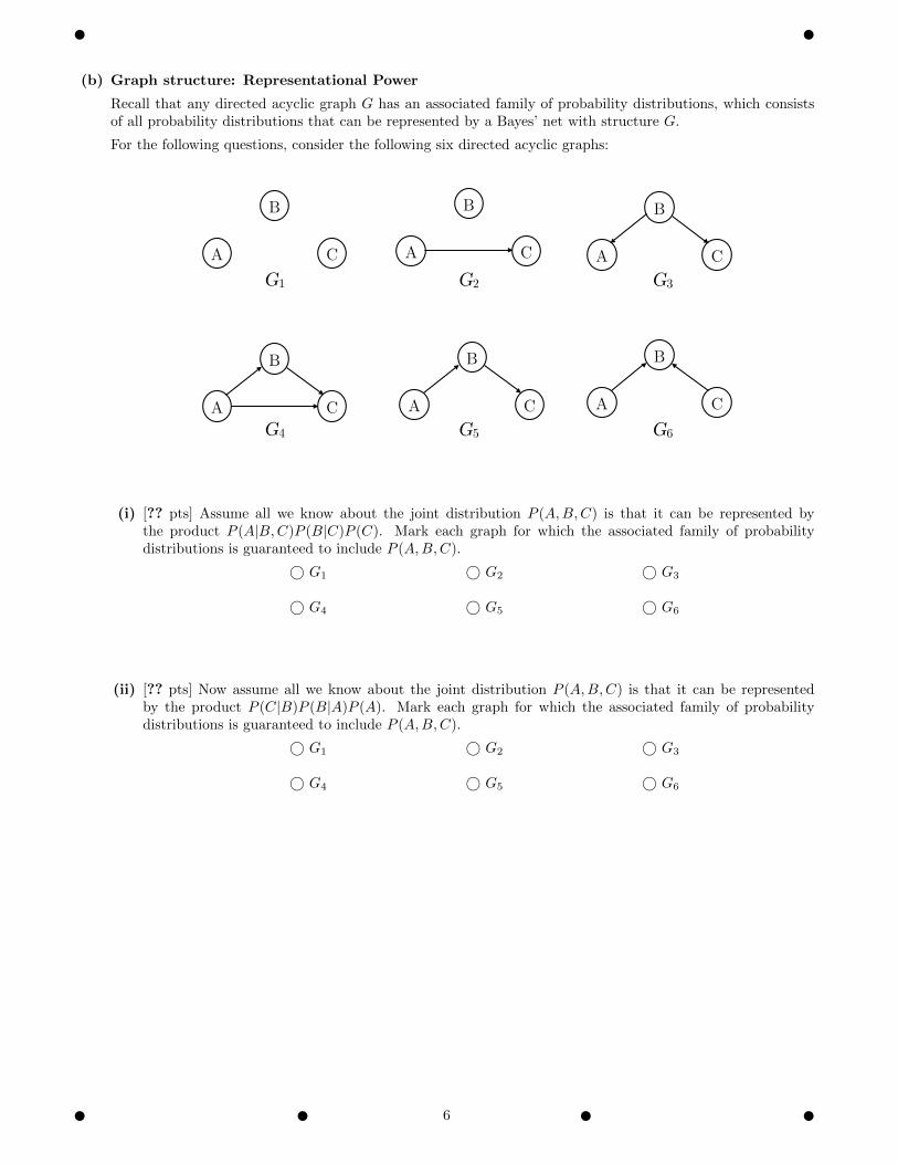
(b) Graph structure: Representational Power

Recall that any directed acyclic graph G has an associated family of probability distributions, which consistsof all probability distributions that can be represented by a Bayes’ net with structure G.

For the following questions, consider the following six directed acyclic graphs:

B

A C

B

A C

B

A C

B

A C

B

A C

B

A C

G1 G2 G3

G4 G5 G6

(i) [?? pts] Assume all we know about the joint distribution P (A,B,C) is that it can be represented bythe product P (A|B,C)P (B|C)P (C). Mark each graph for which the associated family of probabilitydistributions is guaranteed to include P (A,B,C).

© G1 © G2 © G3

© G4 © G5 © G6

(ii) [?? pts] Now assume all we know about the joint distribution P (A,B,C) is that it can be representedby the product P (C|B)P (B|A)P (A). Mark each graph for which the associated family of probabilitydistributions is guaranteed to include P (A,B,C).

© G1 © G2 © G3

© G4 © G5 © G6

6

(c) Marginalization and Conditioning

Consider a Bayes’ net over the random variables A,B,C,D,E with the structure shown below, with full jointdistribution P (A,B,C,D,E).

The following three questions describe different, unrelated situations (your answers to one question should notinfluence your answer to other questions).

BA

C

ED(i) [?? pts] Consider the marginal distribution P (A,B,D,E) =

∑c P (A,B, c,D,E), where C was eliminated.

On the diagram below, draw the minimal number of arrows that results in a Bayes’ net structure that isable to represent this marginal distribution. If no arrows are needed write “No arrows needed.”

BA

ED(ii) [?? pts] Assume we are given an observation: A = a. On the diagram below, draw the minimal number

of arrows that results in a Bayes’ net structure that is able to represent the conditional distributionP (B,C,D,E | A = a). If no arrows are needed write “No arrows needed.”

B

ED

C

(iii) [?? pts] Assume we are given two observations: D = d,E = e. On the diagram below, draw the minimalnumber of arrows that results in a Bayes’ net structure that is able to represent the conditional distributionP (A,B,C | D = d,E = e). If no arrows are needed write “No arrows needed.”

BAC

7

Q3. [?? pts] Variable Elimination

For the Bayes’ net shown on the right, we are given the query P (B,D |+f). All variables have binary domains. Assume we run variableelimination to compute the answer to this query, with the followingvariable elimination ordering: A, C, E, G.

B C

D E F G

A

(a) Complete the following description of the factors generated in this process:

After inserting evidence, we have the following factors to start out with:

P (A), P (B|A), P (C|B), P (D|C), P (E|C,D), P (+f |C,E), P (G|C,+f)

When eliminating A we generate a new factor f1 as follows:

f1(B) =∑a

P (a)P (B|a)

This leaves us with the factors:

P (C|B), P (D|C), P (E|C,D), P (+f |C,E), P (G|C,+f), f1(B)

(i) [?? pts] When eliminating C we generate a new factor f2 as follows:

This leaves us with the factors:

(ii) [?? pts] When eliminating E we generate a new factor f3 as follows:

This leaves us with the factors:

(iii) [?? pts] When eliminating G we generate a new factor f4 as follows:

This leaves us with the factors:

(b) [?? pts] Explain in one sentence how P (B,D|+ f) can be computed from the factors left in part (iii) of (a)?

(c) [?? pts] Among f1, f2, . . . , f4, which is the largest factor generated, and how large is it? Assume all variableshave binary domains and measure the size of each factor by the number of rows in the table that would representthe factor.

For your convenience, the Bayes’ net from the previous page is shown again below.

8

B C

D E F G

A

(d) [?? pts] Find a variable elimination ordering for the same query, i.e., for P (B,D | +f), for which the maximumsize factor generated along the way is smallest. Hint: the maximum size factor generated in your solutionshould have only 2 variables, for a table size of 22 = 4. Fill in the variable elimination ordering and the factorsgenerated into the table below.

Variable Eliminated Factor Generated

For example, in the naive ordering we used earlier, the first line in this table would have had the following twoentries: A, f1(B). For this question there is no need to include how each factor is computed, i.e., no need to includeexpressions of the type =

∑a P (a)P (B|a).

9

Q4. [?? pts] Bayes’ Nets SamplingAssume the following Bayes’ net, and the corresponding distributions over the variables in the Bayes’ net:

BA C DP (B|A)

�a �b 2/3�a +b 1/3+a �b 4/5+a +b 1/5

P (A)�a 3/4+a 1/4

P (C|B)�b �c 1/4�b +c 3/4+b �c 1/2+b +c 1/2

P (D|C)�c �d 1/8�c +d 7/8+c �d 5/6+c +d 1/6

(a) You are given the following samples:

+a + b − c − d+a − b + c − d−a + b + c − d−a − b + c − d

+a − b − c + d+a + b + c − d−a + b − c + d−a − b + c − d

(i) [?? pts] Assume that these samples came from performing Prior Sampling, and calculate the sampleestimate of P (+c).

(ii) [?? pts] Now we will estimate P (+c | +a,−d). Above, clearly cross out the samples that would not beused when doing Rejection Sampling for this task, and write down the sample estimate of P (+c | +a,−d)below.

(b) [?? pts] Using Likelihood Weighting Sampling to estimate P (−a | +b,−d), the following samples were obtained.Fill in the weight of each sample in the corresponding row.

Sample Weight

−a + b + c − d

+a + b + c − d

+a + b − c − d

−a + b − c − d

(c) [?? pts] From the weighted samples in the previous question, estimate P (−a | +b,−d).

(d) [?? pts] Which query is better suited for likelihood weighting, P (D | A) or P (A | D)? Justify your answer inone sentence.

10

(e) [?? pts] Recall that during Gibbs Sampling, samples are generated through an iterative process.

Assume that the only evidence that is available is A = +a. Clearly fill in the circle(s) of the sequence(s) belowthat could have been generated by Gibbs Sampling.

© Sequence 1

1 : +a −b −c +d2 : +a −b −c +d3 : +a −b +c +d

© Sequence 2

1 : +a −b −c +d2 : +a −b −c −d3 : −a −b −c +d

© Sequence 3

1 : +a −b −c +d2 : +a −b −c −d3 : +a +b −c −d

© Sequence 4

1 : +a −b −c +d2 : +a −b −c −d3 : +a +b −c +d

11

Q5. [?? pts] Probability and Decision NetworksThe new Josh Bond Movie (M), Skyrise, is premiering later this week. Skyrise will either be great (+m) or horrendous(−m); there are no other possible outcomes for its quality. Since you are going to watch the movie no matter what,your primary choice is between going to the theater (theater) or renting (rent) the movie later. Your utility ofenjoyment is only affected by these two variables as shown below:

M P(M)+m 0.5-m 0.5

M A U(M,A)+m theater 100-m theater 10

+m rent 80-m rent 40

(a) [?? pts] Maximum Expected Utility

Compute the following quantities:

EU(theater) =

EU(rent) =

MEU({}) =

Which action achieves MEU({}) =

12

(b) [?? pts] Fish and Chips

Skyrise is being released two weeks earlier in the U.K. than the U.S., which gives you the perfect opportunityto predict the movie’s quality. Unfortunately, you don’t have access to many sources of information in theU.K., so a little creativity is in order.

You realize that a reasonable assumption to make is that if the movie (M) is great, citizens in the U.K. willcelebrate by eating fish and chips (F ). Unfortunately the consumption of fish and chips is also affected by apossible food shortage (S), as denoted in the below diagram.

The consumption of fish and chips (F ) and the food shortage (S) are both binary variables. The relevantconditional probability tables are listed below:

S M F P (F |S,M)+s +m +f 0.6+s +m -f 0.4+s -m +f 0.0+s -m -f 1.0

S M F P (F |S,M)-s +m +f 1.0-s +m -f 0.0-s -m +f 0.3-s -m -f 0.7

S P (S)+s 0.2-s 0.8

You are interested in the value of revealing the food shortage node (S). Answer the following queries:

EU(theater|+ s) =

EU(rent|+ s) =

MEU({+s}) =

Optimal Action Under {+s} =

MEU({−s}) =

Optimal Action Under {−s} =

V PI(S) =

13

(c) [?? pts] Greasy Waters

You are no longer concerned with the food shortage variable. Instead, you realize that you can determinewhether the runoff waters are greasy (G) in the U.K., which is a variable that indicates whether or not fishand chips have been consumed. The prior on M and utility tables are unchanged. Given this different modelof the problem:

G F P (G|F )+g +f 0.8-g +f 0.2

+g -f 0.3-g -f 0.7

F M P (F |M)+f +m 0.92-f +m 0.08

+f -m 0.24-f -m 0.76

M P(M)+m 0.5-m 0.5

M A U(M,A)+m theater 100-m theater 10

+m rent 80-m rent 40

[Decision network] [Tables that define the model]

F P (F )+f 0.58-f 0.42

G P (G)+g 0.59-g 0.41

M G P (M |G)+m +g 0.644-m +g 0.356

+m -g 0.293-m -g 0.707

G M P (G|M)+g +m 0.760-g +m 0.240

+g -m 0.420-g -m 0.580

M F P (M |F )+m +f 0.793-m +f 0.207

+m -f 0.095-m -f 0.905

[Tables computed from the first set of tables. Some of them might be convenient to answer the questions below]

Answer the following queries:

MEU(+g) =

MEU(−g) =

V PI(G) =

14

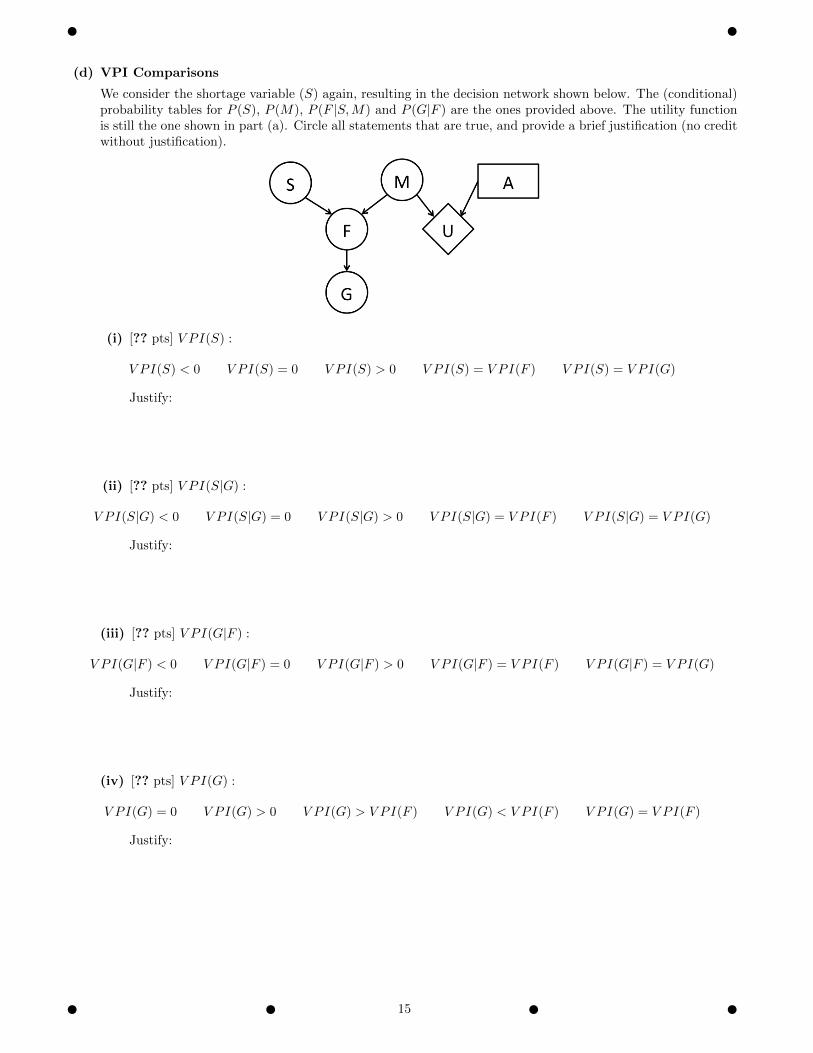
(d) VPI Comparisons

We consider the shortage variable (S) again, resulting in the decision network shown below. The (conditional)probability tables for P (S), P (M), P (F |S,M) and P (G|F ) are the ones provided above. The utility functionis still the one shown in part (a). Circle all statements that are true, and provide a brief justification (no creditwithout justification).

(i) [?? pts] V PI(S) :

V PI(S) < 0 V PI(S) = 0 V PI(S) > 0 V PI(S) = V PI(F ) V PI(S) = V PI(G)

Justify:

(ii) [?? pts] V PI(S|G) :

V PI(S|G) < 0 V PI(S|G) = 0 V PI(S|G) > 0 V PI(S|G) = V PI(F ) V PI(S|G) = V PI(G)

Justify:

(iii) [?? pts] V PI(G|F ) :

V PI(G|F ) < 0 V PI(G|F ) = 0 V PI(G|F ) > 0 V PI(G|F ) = V PI(F ) V PI(G|F ) = V PI(G)

Justify:

(iv) [?? pts] V PI(G) :

V PI(G) = 0 V PI(G) > 0 V PI(G) > V PI(F ) V PI(G) < V PI(F ) V PI(G) = V PI(F )

Justify:

15

Q6. [?? pts] ElectionThe country of Purplestan is preparing to vote on its next President! In this election, the incumbent PresidentPurple is being challenged by the ambitious upstart Governor Fuschia. Purplestan is divided into two states of equalpopulation, Redexas and Blue York, and the Blue York Times has recruited you to help track the election.

Rt+1

Bt+1Bt

Rt

SRt SB

t

SNt

SNt+1

SRt+1 SB

t+1

Drift and Error Models

x D(x) ER(x) EB(x) EN (x)5 .01 .00 .04 .004 .03 .01 .06 .003 .07 .04 .09 .012 .12 .12 .11 .051 .17 .18 .13 .240 .20 .30 .14 .40-1 .17 .18 .13 .24-2 .12 .12 .11 .05-3 .07 .04 .09 .01-4 .03 .01 .06 .00-5 .01 .00 .04 .00

To begin, you draw the dynamic Bayes net given above, which includes the President’s true support in Redexas andBlue York (denoted Rt and Bt respectively) as well as weekly survey results. Every week there is a survey of eachstate, SR

t and SBt , and also a national survey SN

t whose sample includes equal representation from both states.

The model’s transition probabilities are given in terms of the random drift model D(x) specified in the table above:

P (Rt+1|Rt) = D(Rt+1 −Rt)

P (Bt+1|Bt) = D(Bt+1 −Bt)

Here D(x) gives the probability that the support in each state shifts by x between one week and the next. Similarly,the observation probabilities are defined in terms of error models ER(x), EB(x), and EN (x):

P (SRt |Rt) = ER(SR

t −Rt)

P (SBt |Bt) = EB(SB

t −Bt)

P (SNt |Rt, Bt) = EN

(SNt −

Rt + Bt

2

)where the error model for each survey gives the probability that it differs by x from the true support; the differenterror models represent the surveys’ differing polling methodologies and sample sizes. Note that SN

t depends on bothRt and Bt, since the national survey gives a noisy average of the President’s support across both states.

(a) Particle Filtering. First we’ll consider using particle filtering to track the state of the electorate. Throughoutthis problem, you may give answers either as unevaluated numeric expressions (e.g. 0.4 · 0.9) or as numericvalues (e.g. 0.36).

(i) [?? pts] Suppose we begin in week 1 with the two particles listed below. Now we observe the first week’ssurveys: SR

1 = 51, SB1 = 45, and SN

1 = 50. Write the weight of each particle given this evidence:

Particle Weight

(r = 49, b = 47)

(r = 52, b = 48)

16

The figures and table below are identical to the ones on the previous page and are repeated here for yourconvenience.

Rt+1

Bt+1Bt

Rt

SRt SB

t

SNt

SNt+1

SRt+1 SB

t+1

Drift and Error Models

x D(x) ER(x) EB(x) EN (x)5 .01 .00 .04 .004 .03 .01 .06 .003 .07 .04 .09 .012 .12 .12 .11 .051 .17 .18 .13 .240 .20 .30 .14 .40-1 .17 .18 .13 .24-2 .12 .12 .11 .05-3 .07 .04 .09 .01-4 .03 .01 .06 .00-5 .01 .00 .04 .00

(ii) [?? pts] Now we resample the particles based on their weights; suppose our resulting particle set turns outto be {(r = 52, b = 48), (r = 52, b = 48)}. Now we pass the first particle through the transition model toproduce a hypothesis for week 2. What’s the probability that the first particle becomes (r = 50, b = 48)?

(iii) [?? pts] In week 2, disaster strikes! A hurricane knocks out the offices of the company performing the BlueYork state survey, so you can only observe SR

2 = 48 and SN2 = 50 (the national survey still incorporates

data from voters in Blue York). Based on these observations, compute the weight for each of the twoparticles:

Particle Weight

(r = 50, b = 48)

(r = 49, b = 53)

17

(iv) [?? pts] Your editor at the Times asks you for a “now-cast” prediction of the election if it were heldtoday. The election directly measures the true support in both states, so R2 would be the election resultin Redexas and Bt the result in Blue York.

To simplify notation, let I2 = (SR1 , SB

1 , SN1 , SR

2 , SN2 ) denote all of the information you observed in weeks

1 and 2, and also let the variable Wi indicate whether President Purple would win an election in week i:

Wi =

{1 if Ri+Bi

2 > 500 otherwise.

For improved accuracy we will work with the weighted particles rather than resampling. Normally wewould build on top of step (iii), but to decouple errors, let’s assume that after step (iii) you ended up withthe following weights:

Particle Weight

(r = 50, b = 48) .12

(r = 49, b = 53) .18

Note this is not actually what you were supposed to end up with! Using the weights from this table,estimate the following quantities:

• The current probability that the President would win:

P (W2 = 1|I2) ≈

• Expected support for President Purple in Blue York:

E[B2|I2] ≈

(v) [?? pts] The real election is being held next week (week 3). Suppose you are representing the currentjoint belief distribution P (R2, B2|I2) with a large number of unweighted particles. Explain using no morethan two sentences how you would use these particles to forecast the national election (i.e. how you wouldestimate P (W3 = 1|I2), the probability that the President wins in week 3, given your observations fromweeks 1 and 2).

18

Q7. [?? pts] Naive Bayes’ Modeling AssumptionsYou are given points from 2 classes, shown as rectangles and dots. For each of the following sets of points, markif they satisfy all the Naive Bayes’ modelling assumptions, or they do not satisfy all the Naive Bayes’ modellingassumptions. Note that in (c), 4 rectangles overlap with 4 dots.

−1 0 1 2 3

−1

−0.5

0

0.5

1

1.5

2

2.5

3

f1

f 2

(a) © Satisfies © Does not Satisfy

−0.5 0 0.5 1 1.5 2

−2

−1.5

−1

−0.5

0

f1

f 2

(b) © Satisfies © Does not Satisfy

0 0.5 1

−2

−1.8

−1.6

−1.4

−1.2

−1

−0.8

−0.6

−0.4

−0.2

f1

f 2

(c) © Satisfies © Does not Satisfy

−0.5 0 0.5 1 1.5 2

−2

−1.5

−1

−0.5

0

0.5

f1

f 2

(d) © Satisfies © Does not Satisfy

−1 0 1 2 3

−1

−0.5

0

0.5

1

1.5

2

2.5

3

3.5

f1

f 2

(e) © Satisfies © Does not Satisfy

−1.5 −1 −0.5 0 0.5 1 1.5 2 2.5 3

−1

−0.5

0

0.5

1

1.5

2

f1

f 2

(f) © Satisfies © Does not Satisfy

19

Q8. [?? pts] Model Structure and Laplace SmoothingWe are estimating parameters for a Bayes’ net with structure GA and for a Bayes’ net with structure GB . To estimatethe parameters we use Laplace smoothing with k = 0 (which is the same as maximum likelihood), k = 5, and k =∞.

AG BG

Let for a given Bayes’ net BN the corresponding joint distribution over all variables in the Bayes’ net be PBN thenthe likelihood of the training data for the Bayes’ net BN is given by∏

xi∈Training Set

PBN (xi)

Let L0A denote the likelihood of the training data for the Bayes’ net with structure GA and parameters learned with

Laplace smoothing with k = 0.Let L5

A denote the likelihood of the training data for the Bayes’ net with structure GA and parameters learned withLaplace smoothing with k = 5.Let L∞

A denote the likelihood of the training data for the Bayes’ net with structure GA and parameters learned withLaplace smoothing with k =∞.We similarly define L0

B , L5B , L∞

B for structure GB .

For each of the questions below, mark which one is the correct option.

(a) [?? pts] Consider L0A and L5

A

© L0A ≤ L5

A © L0A ≥ L5

A © L0A = L5

A © Insufficient information to determine the ordering.

(b) [?? pts] Consider L5A and L∞

A

© L5A ≤ L∞

A © L5A ≥ L∞

A © L5A = L∞

A © Insufficient information to determine the ordering.

(c) [?? pts] Consider L0B and L∞

B

© L0B ≤ L∞

B © L0B ≥ L∞

B © L0B = L∞

B © Insufficient information to determine the ordering.

(d) [?? pts] Consider L0A and L0

B

© L0A ≤ L0

B © L0A ≥ L0

B © L0A = L0

B © Insufficient information to determine the ordering.

(e) [?? pts] Consider L∞A and L∞

B

© L∞A ≤ L∞

B © L∞A ≥ L∞

B © L∞A = L∞

B © Insufficient information to determine the ordering.

(f) [?? pts] Consider L5A and L0

B

© L5A ≤ L0

B © L5A ≥ L0

B © L5A = L0

B © Insufficient information to determine the ordering.

(g) [?? pts] Consider L0A and L5

B

© L0A ≤ L5

B © L0A ≥ L5

B © L0A = L5

B © Insufficient information to determine the ordering.

20

Q9. [?? pts] ML: Short Question & Answer(a) Parameter Estimation and Smoothing. For the Bayes’ net drawn on the left, A can take on values +a,−a, and B can take values +b and −b. We are given samples (on the right), and we want to use them toestimate P (A) and P (B|A).

A B

(−a, +b)

(−a, −b)(−a, +b)

(−a, +b)

(−a, −b)(−a, −b)

(−a, −b)(−a, +b)

(+a, +b)

(−a, −b)

(i) [?? pts] Compute the maximum likelihood estimates for P (A)and P (B|A), and fill them in the 2 tables on the right.

A P (A)+a

-a

A B P (B|A)+a +b

+a -b

-a +b

-a -b

(ii) [?? pts] Compute the estimates for P (A) and P (B|A) usingLaplace smoothing with strength k = 2, and fill them in the2 tables on the right.

A P (A)+a

-a

A B P (B|A)+a +b

+a -b

-a +b

-a -b

(b) [?? pts] Linear Separability. You are given samples from 2 classes (. and +) with each sample being describedby 2 features f1 and f2. These samples are plotted in the following figure. You observe that these samples arenot linearly separable using just these 2 features. Circle the minimal set of features below that you could usealongside f1 and f2, to linearly separate samples from the 2 classes.

−2 −1 0 1 2−2

−1.5

−1

−0.5

0

0.5

1

1.5

2

f1

f 2

© f1 < 1.5

© f1 > 1.5

© f1 < −1.5

© f1 > −1.5

© f2 < 1

© f2 > 1

© f2 < −1

© f2 > −1

©f21

©f22

©|f1 + f2|

© Even using all these features alongside f1 and f2 will not make the sampleslinearly separable.

(c) [?? pts] Perceptrons. In this question you will perform perceptron updates. You have 2 classes, +1 and −1,and 3 features f0, f1, f2 for each training point. The +1 class is predicted if w · f > 0 and the −1 class ispredicted otherwise.

You start with the weight vector, w = [1 0 0]. In the table below, do a perceptron update for each ofthe given samples. If the w vector does not change, write No Change, otherwise write down the new w vector.

f0 f1 f2 Class Updated w

1 7 8 -1

1 6 8 -1

1 9 6 +1

21