CS 229 | Classification of Channel Bifurcation Points in Remote Sensing Imagery of River Deltas

Erik Nesvold |nesvold@stanford.edu

I. Introduction River deltas are very important landforms on Earth that are both home to about 500 million people

[1] and deliver essential nutrients and sediments to the extremely diverse ecosystems within them.

With a rising sea level due to climate change and other anthropogenic impact, such as dam

construction and river engineering, both human life and the ecosystems in deltas have become

increasingly vulnerable over the past century. There is also intense economic interest in deltaic

structural properties since they ultimately become high-quality reservoirs for groundwater,

hydrocarbons and potential CO2 storage.

The idea of characterizing river deltas based on their network properties was first introduced

in 1971 by Smart & Moruzzi, but this analysis mainly focused on the ratio between channel forks

and channel junctions. There has recently been renewed interest in a more formal graph theoretic

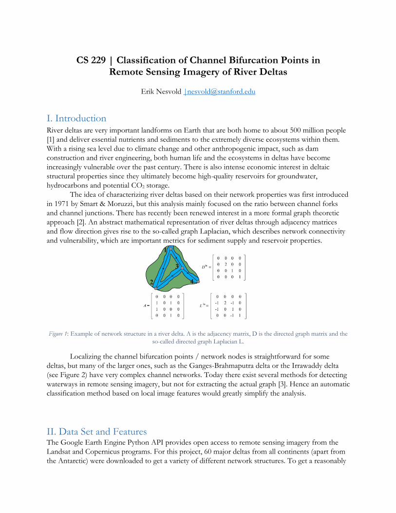
approach [2]. An abstract mathematical representation of river deltas through adjacency matrices

and flow direction gives rise to the so-called graph Laplacian, which describes network connectivity

and vulnerability, which are important metrics for sediment supply and reservoir properties.

Figure 1: Example of network structure in a river delta. A is the adjacency matrix, D is the directed graph matrix and the

so-called directed graph Laplacian L.

Localizing the channel bifurcation points / network nodes is straightforward for some

deltas, but many of the larger ones, such as the Ganges-Brahmaputra delta or the Irrawaddy delta

(see Figure 2) have very complex channel networks. Today there exist several methods for detecting

waterways in remote sensing imagery, but not for extracting the actual graph [3]. Hence an automatic

classification method based on local image features would greatly simplify the analysis.

II. Data Set and Features The Google Earth Engine Python API provides open access to remote sensing imagery from the

Landsat and Copernicus programs. For this project, 60 major deltas from all continents (apart from

the Antarctic) were downloaded to get a variety of different network structures. To get a reasonably

large training dataset, 560 bifurcation points were identified and labeled manually. In the images

where the bifurcation points were exhaustively labeled, a total of 1400 regular points were extracted

as well. A 61x61 pixel region around each point was used for classification, where the region size

was found using cross validation. Because of the different scales involved, it was expected that the

region size should vary as a function of the local channel size, but the error rate turned out to be

lower when it was fixed.

Figure 2: A subsection of the Irrawaddy Delta in South-East Asia (Landsat 8 imagery from Google Earth Engine, 53 x 55

km) with expected flow direction shown with blue vectors. Some bifurcation points are shown in the red box - which

illustrates the complexity of the channel network.

The NDWI index is the normalized difference between the green and the infrared bandwidth, and is

used to detect presence of water in remote sensing imagery. There exist several methods to find

network structures such as roads and rivers, but not to extract the topology of the graph. In this

case, a singularity index based on image gradients computed over the range of scales of interest gave

good results [3] – so these two pre-processing steps return a 2D binary image of the river network –

see figure 3. Furthermore, it is then possible to compute channel centerlines, expected flow

directions and local channel widths. These features were subsequently used as data dimensions to

traditional classification methods.

III. Machine Learning Methods and Implementation DetailsOne challenge with using images as a dataset is obviously that the dataset is not immediately in the

familiar form of rows and columns corresponding to observations and predictors. Two main

approaches were used: (i) classification based directly on features in the images and (ii) feature

engineering in combination with a ‘traditional’ classifier.

Classification Based Directly on Images

There are several methods available for recognizing template images, e.g. similarly to PCA and ICA

for facial recognition. However, there is a large variety in the visual appearance of the channel

bifurcation points, so the idea of using a template image for recognition was not pursued further. It

may be possible to create multiple templates, but this would probably also increase the false positive

rate (at least for classification methods that do not return probabilities, such as SVM).

Figure 3: Features in the local region around a manually labeled bifurcation point. The top left image is the NDWI index,

which highlights reflection of water. Troublesome features such as clouds are sometimes present.

Deep Learning / Convolutional Neural Networks is an attractive approach since it does not

require feature engineering, but due to the relatively small set of training images available and the

lack of GPU resources available, this was deemed infeasible at this point. Instead, automatic feature

descriptors such as histograms of oriented gradients (HOG) [4], GIST [5] and image features from

scale-invariant key points (SIFT) [6] were considered as a more interesting approach. These methods

are similar in several respects; e.g. they break up the original image in bins and compute image

gradients. But whereas GIST is a global image descriptor, HOG and SIFT are used to find localized

features, such as pedestrians. Figure 4 shows HOG features for the bifurcation point shown in

Figure 3.

Figure 4: From left to right; original input image, GIST features and HOG features for the same 61 x 61 pixel region as

in Figure 3.

These methods were used because there seem to be both local and global characteristics of the

bifurcation points, such as the presence of a dividing river bank, a connected water body with one or

more branches etc. In other words, much of the information should lie in abrupt gradients at fine

scales, which is precisely the motivation behind HOG. The cell sizes were found using tenfold cross-

validation. After extracting the image features, the same classifiers were used as for the manually

extracted features.

Classification Based on Features in the Images

Based on a visual inspection of the local regions around each point, there seem to be many features that can help distinguish channel bifurcation points from regular points. The following numerical features are computed in the region around each candidate point:

K-means clustering (with k = 3) of the computed flow directions in the surrounding region within the channels. The underlying assumption is that three distinct channels should generate three different distributions of the angle of flow.

The ratio of the velocity at the candidate point to the mean velocity in the region - right in front of a dividing piece of land the water velocity should be lower than in the center of the channels.

The fraction of water in the image

The number of connected water bodies within the image and the number of land bodies.

The number of bodies at the edge of the image that are connected to the candidate point

K-means clustering (with k = 3) of the channel widths. These nine features are then standardized and tested with several standard classification methods:

SVM with and without the following kernels:

o Radial basis function / Gaussian kernel: 𝐾(𝑥, 𝑦) = exp(−‖𝑥−𝑦‖2

2𝜎2)

o Polynomial kernel: 𝐾(𝑥, 𝑦) = (1 + 𝑥′𝑦)𝑑

Multinomial logistic regression: softmax(𝑘, 𝒙) =exp(βk

′ 𝑥𝑘)

1+∑exp(βi′𝑥𝑖)

Gaussian Discriminant Analysis: the probabilities are computed based on the log ratio:

logP(𝐺=1|𝑋=𝑥)

P(𝐺=0|𝑋=𝑥)= log

𝜋1

𝜋0−

1

2(𝜇1 + 𝜇0)

′𝛴−1(𝜇1 − 𝜇0) + 𝑥′𝛴−1(𝜇1 − 𝜇0), where the class

prior is computed empirically from the data.

Decision tree with boosting: Adaboost M1 [7], which adjusts adaptively to the errors of the weak hypotheses. Adaboost was developed by Freund and Schapire for the example of a gambler with several weak strategies, and is considered as a good off-the shelf version of boosted decision trees. The standard version in Matlab uses 100 trees. Intuitively, it seems like a combination of weak learners, such as whether there are three water bodies at the edge of the region around the candidate point, that might work well for this problem.

IV. ResultsThe methods were evaluated in terms of overall error rate, computational time and perhaps most

importantly, the false positive rate. This is because there are many more normal points than actual

bifurcation points. Methods that return probabilities, such as logistic regression and GDA are

advantageous because this makes it possible to plot the ROC curve. However, kernel SVM

performed much better than both GDA and logistic regression, which in all cases had error rates

over 20%. For all methods, 10-fold cross-validation was used to optimize free parameters, such as

the variance of the Gaussian kernel and the maximum tree depths. However, this type of

optimization rarely showed significant differences – changing tree depths in Adaboost and the prior

model for GDA resulted in insignificant improvements compared to the differences between

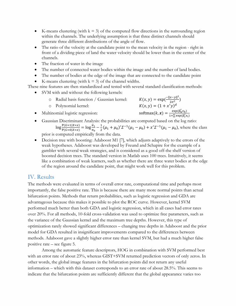
methods. Adaboost gave a slightly higher error rate than kernel SVM, but had a much higher false

positive rate – see figure 5.

Among the automatic feature descriptors, HOG in combination with SVM performed best

with an error rate of about 23%, whereas GIST+SVM returned prediction vectors of only zeros. In

other words, the global image features in the bifurcation points did not return any useful

information – which with this dataset corresponds to an error rate of about 28.5%. This seems to

indicate that the bifurcation points are sufficiently different that the global appearance varies too

much to be useful – whereas HOG, that emphasizes the local gradients gives some valuable

information. Still, the results from using the engineered features were much better; errors of 7.5%

and 11.5% for Gaussian kernel SVM and Adaboost, respectively. This seems to indicate that expert

knowledge about the physical process in combination with a good statistical classifier gives better

results than something based purely on the image characteristics.

The computational time was not too high to evaluate on the order of 104 points along the

channel centerlines for each delta for any of the methods, and by imposing a minimum distance

between bifurcation points it is possible to avoid getting on the order of 500 false positive points for

each satellite image– see the example output of the classifier in figure 6.

Figure 5: Confusion matrices for the three methods that gave the best results; from left to right (i) engineered features + kernel SVM, (ii) engineered features + Adaboost, (iii) HOG+SVM. The negative case (0) corresponds to the top row and the positive case (1) to the bottom row. SVM with a Gaussian kernel is seen to give a lower false positive rate (in red) than the other methods and had the lowest overall error rate; 7.5 %. The error is computed using randomized

permutation of the dataset, 10-fold cross validation and a 0/1 error.

V. Discussion The bulk of the work was the file creation and labeling of the data, since, to this author’s best

knowledge, no such automatic classification has been performed earlier. Once the data was in the

familiar form of a matrix of predictors X and a vector of labels y, classification was relatively

straightforward. The emphasis was on testing several different methods since the author was very

uncertain what type of approach would be optimal for this problem. Given the large variety of

bifurcation points, HOG features worked surprisingly well. Before computing the deltaic network

graphs in this research project, other automatic feature descriptors will be tested as well (such as

SIFT). Adding more engineered features is also an option, since it is not necessarily intuitive which

features distinguish the classes – e.g. somewhat surprisingly, the fraction of water in the local region

around the candidate point reduced the test error by 2 %. However, the error rate is already low

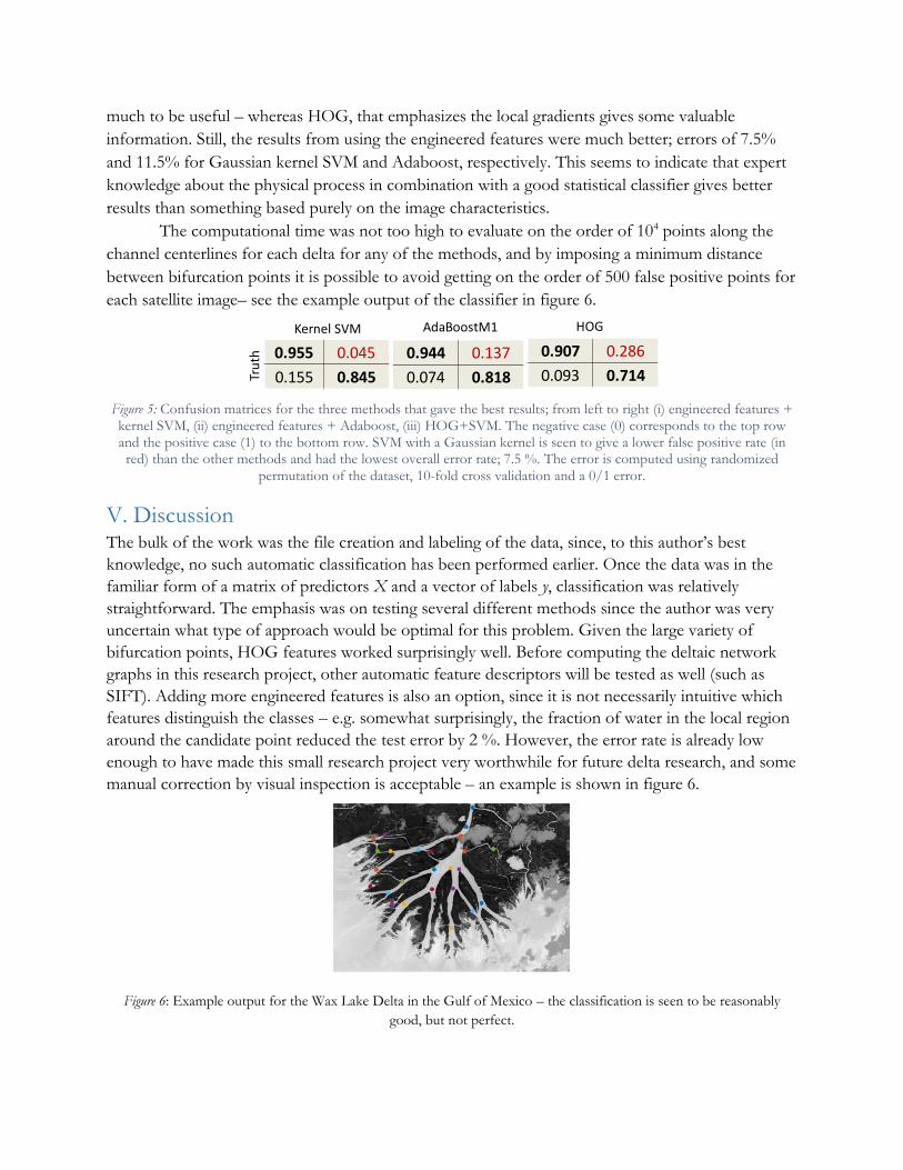
enough to have made this small research project very worthwhile for future delta research, and some

manual correction by visual inspection is acceptable – an example is shown in figure 6.

Figure 6: Example output for the Wax Lake Delta in the Gulf of Mexico – the classification is seen to be reasonably

good, but not perfect.

0.955 0.045

0.155 0.845

0.907 0.286

0.093 0.714

KernelSVM HOG

Truth 0.944 0.137

0.074 0.818

AdaBoostM1

Bibliography

[1] T. Agardi and J. Alder, "Coastal Systems," in Ecosystems and Human Well-Being: Current State and Trends, Washington DC, Island Press, 2005.

[2] A. Tejedor, "Delta channel networks: 1. A graph-theoretic approach for studying connectivity and steady state transport on deltaic surfaces," AGU Water Resources Research , pp. 3998-4020, 2015.

[3] F. Isikdogan, A. C. Bovik and P. Passalacqua, "Automatic channel network extraction from remotely sensed images by singularity analysis," IEEE Geoscience and Remote Sensing Letters, pp. 2218-2221, 2015.

[4] N. Dalal, "Histograms of Oriented Gradients for Human Detection," IEEE Computer Society Conference on Computer Vision and Pattern Recognition, vol. 1, pp. 886-893, 2005.

[5] A. Oliva and A. Torralba, "Building the gist of a scene: the role of global image features in recognition," Progress in Brain Research, no. 155, pp. 23-36, 2006.

[6] D. G. Lowe, "Distinctive Image Features from Scale-Invariant Keypoints," International Journal of Computer Vision, vol. 60, no. 2, pp. 91-110, 2004.

[7] Y. Freund and R. E. Schapire, "A decision theoretic generalization of online learning and an application to boosting," Journal of Computer and Systems Sciences, vol. 55, no. 1, pp. 119-139, 1997.