CS 237: Probability in Computing

Wayne SnyderComputer Science Department

Boston University

Lecture 15:• Continuous Distributions

• Basic Definitions

• Importance of the CDF

• Calculation of probabilities using integration

• Uniform Continuous Distribution

• Introduction to Normal Distribution

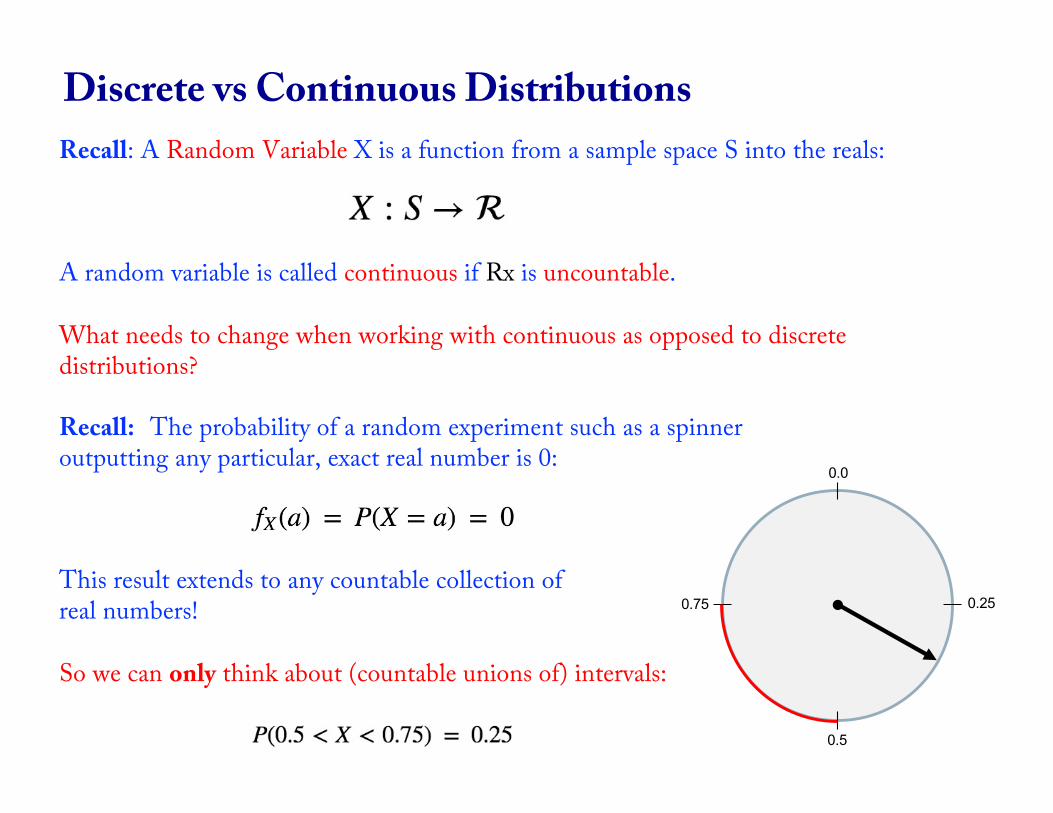
Recall: A Random Variable X is a function from a sample space S into the reals:

A random variable is called continuous if Rx is uncountable.

What needs to change when working with continuous as opposed to discrete distributions?

Recall: The probability of a random experiment such as a spinner outputting any particular, exact real number is 0:

This result extends to any countable collection ofreal numbers!

So we can only think about (countable unions of) intervals:

Discrete vs Continuous Distributions

0.5

0.75 0.25

0.0

When the sample space is uncountable, say with the spinner, it is possible for the probability function to be equiprobable or non-equiprobable.

Uncountable and Equiprobable:

Example: Spin the spinner and report the real number showing.

S = [0..1) Any point is equally likely

Uncountable and NOT Equiprobable:

Example: Heights of Human Beings:

Probability Functions: Equiprobable vs Not Equiprobable

People are more likely to be close to the average height than at the extremes!

Review: Cumulative Distribution Functions

The Cumulative Distribution Function (CDF) for a random variable X shows what happens when we keep track of the sum of the probability distribution from left to right over its range:

Example: X = “The number of dots showing on a thrown die”

Probability Distribution Function PX Cumulative Distribution Function FX

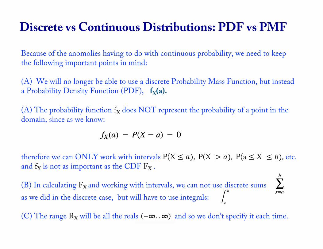
Because of the anomolies having to do with continuous probability, we need to keep the following important points in mind:

(A) We will no longer be able to use a discrete Probability Mass Function, but instead a Probability Density Function (PDF), fX(a).

(A) The probability function fX does NOT represent the probability of a point in the domain, since as we know:

therefore we can ONLY work with intervals P(X ≤ 𝑎), P(X > 𝑎), P(a ≤ X ≤ 𝑏), etc. and fX is not as important as the CDF FX .

(B) In calculating FX and working with intervals, we can not use discrete sums as we did in the discrete case, but will have to use integrals:

(C) The range RX will be all the reals and so we don’t specify it each time.

Discrete vs Continuous Distributions: PDF vs PMF

Discrete vs Continuous Distributions

Discrete Random Variables Continuous Random Variables

The Probability Mass Function (PMF) of a discrete random variable X is a function from the range of X into R :

such that

(i)

(ii)

The Probability Density Function (PDF) of a continuous random variable X is a function from R to R :

such that

(i)

(ii)

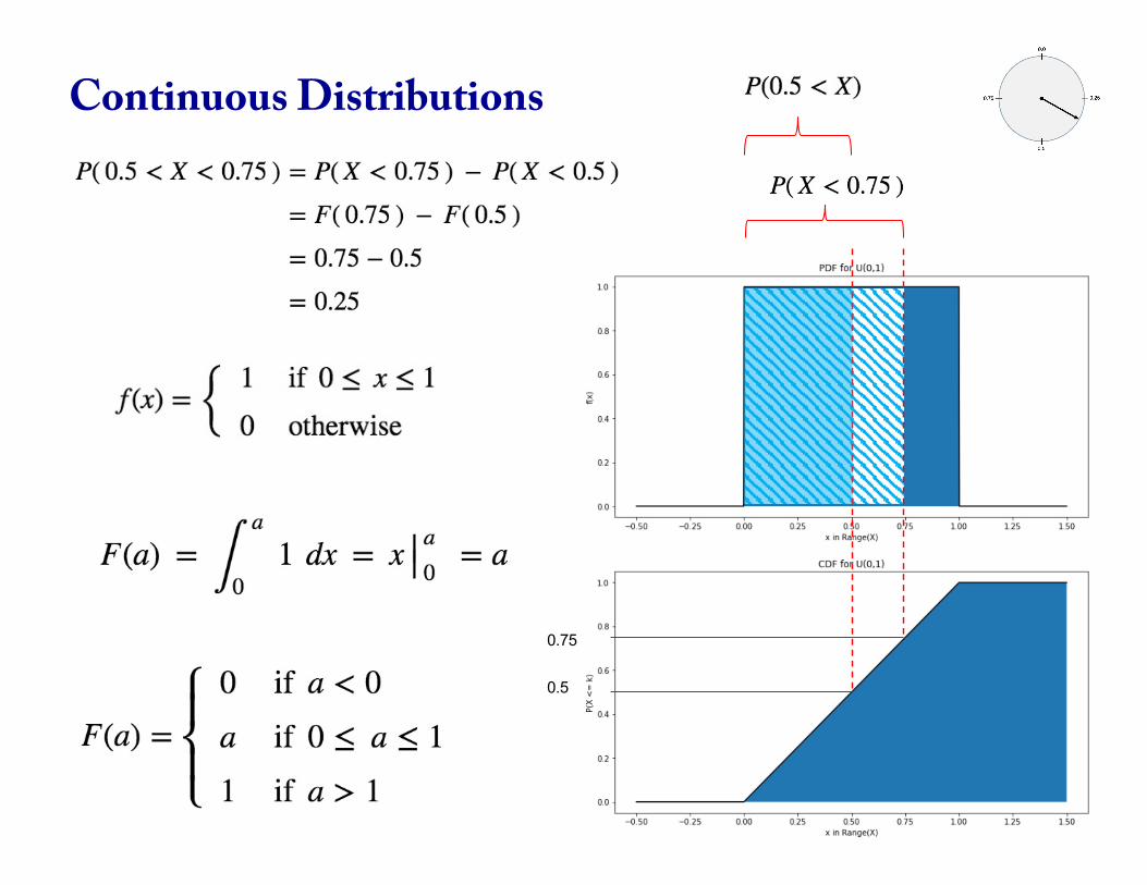
Continuous Distributions

Let’s clarify these ideas with an example....

Consider the spinner example from way back when:

X = “the real number in [0..1) that the spinner lands on”

The probability density function is:

Note that the area is 1.0 and for any 0 ≤ 𝑎 ≤ 1, we have𝑓(𝑎) = 1.0, so it is uniform across [0..1). But clearly P(X = a) = 0.0.

0.0

0.5

0.75 0.25

Continuous Distributions Now recall that the ONLY way to deal with continuous probability is to use intervals and to use area (or extent) for the probability. Hence we will calculate probabilities of intervals using the CDF:

0.75

0.75

A brief review of integration is on the YT channel!

Continuous Distributions

0.75

0.5

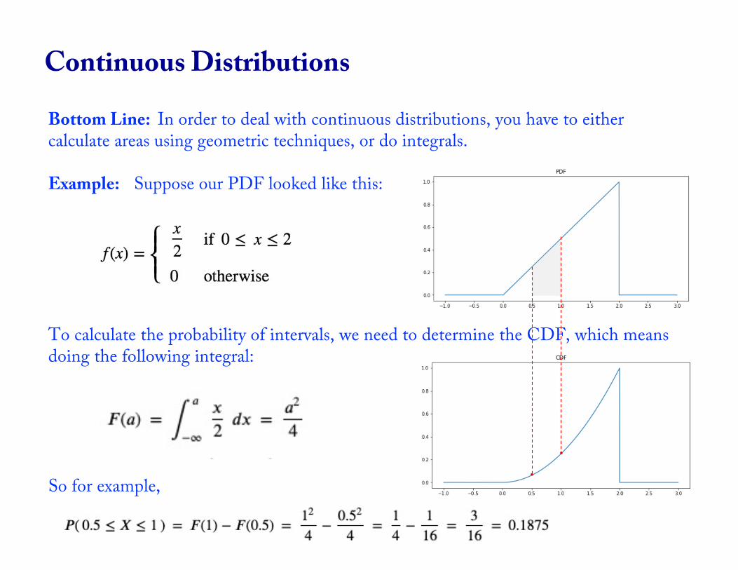
Bottom Line: In order to deal with continuous distributions, you have to either calculate areas using geometric techniques, or do integrals.

Example: Suppose our PDF looked like this:

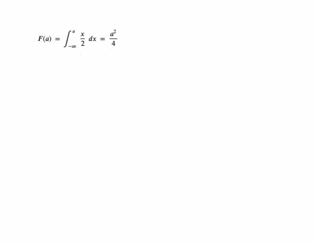
To calculate the probability of intervals, we need to determine the CDF, which means doing the following integral:

So for example,

Continuous Distributions

Continuous Distributions

Discrete Random Variables Continuous Random Variables

Same for both Discrete and Continuous Random Variables

All previous theorems about E(X) and Var(X) still hold, it does not matter whether X is continuous or discrete!

Example: Calculate the expected value of the uniform distribution over the interval [0..1):

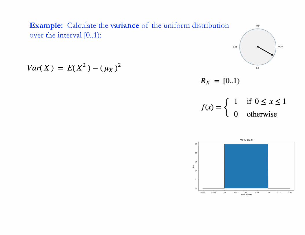
Example: Calculate the variance of the uniform distribution over the interval [0..1):

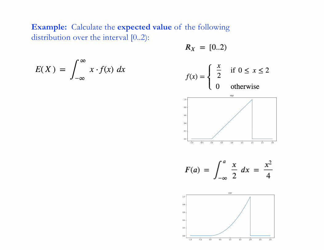
Example: Calculate the expected value of the following distribution over the interval [0..2):

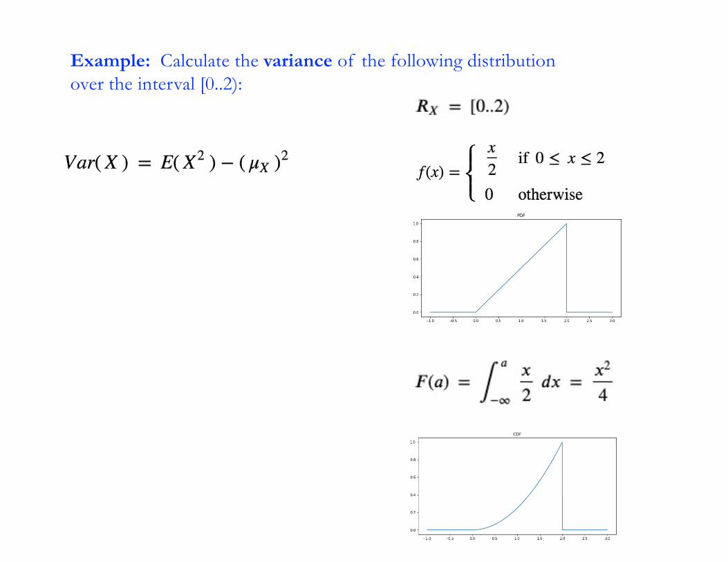
Example: Calculate the variance of the following distribution over the interval [0..2):

Uniform Distribution

19

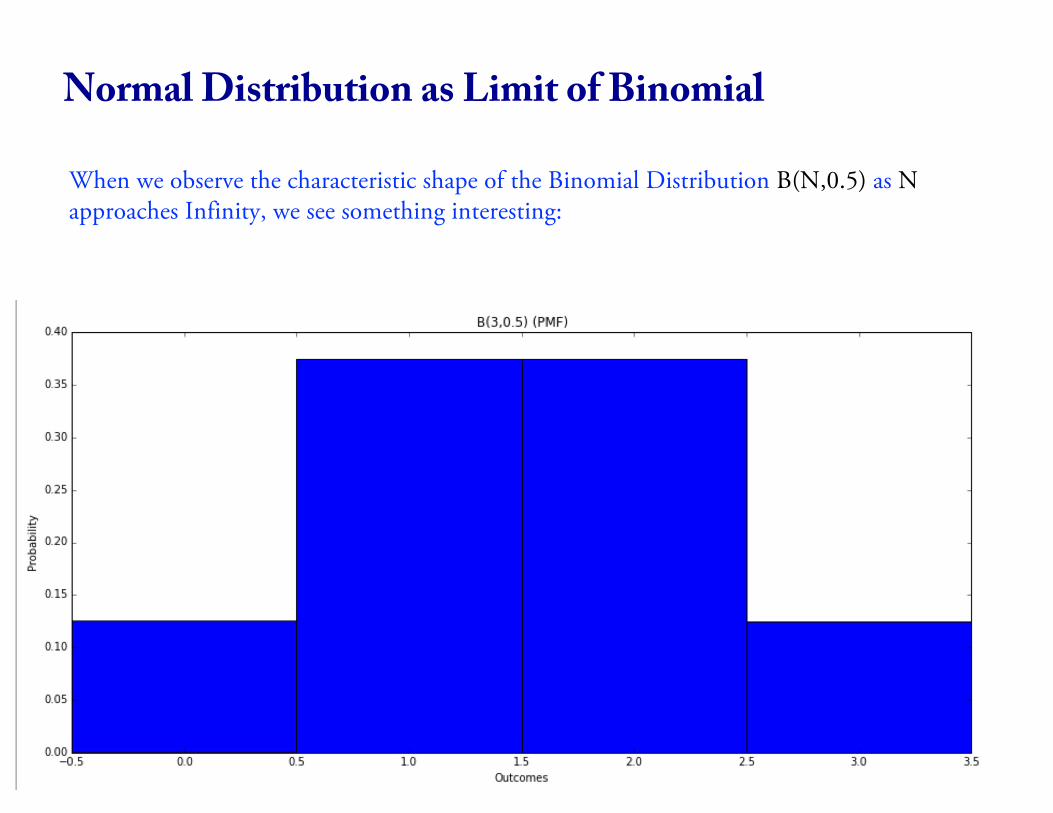
When we observe the characteristic shape of the Binomial Distribution B(N,0.5) as Napproaches Infinity, we see something interesting:

Normal Distribution as Limit of Binomial

20

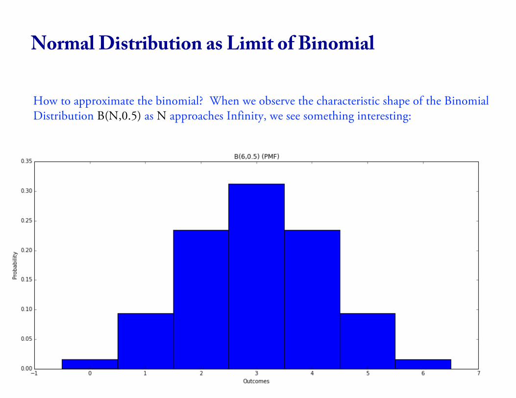
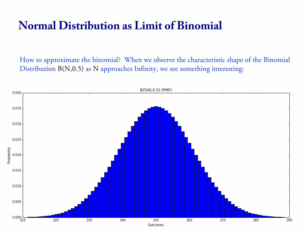
How to approximate the binomial? When we observe the characteristic shape of the Binomial Distribution B(N,0.5) as N approaches Infinity, we see something interesting:

Normal Distribution as Limit of Binomial

21

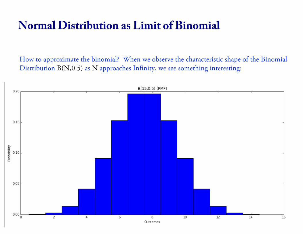
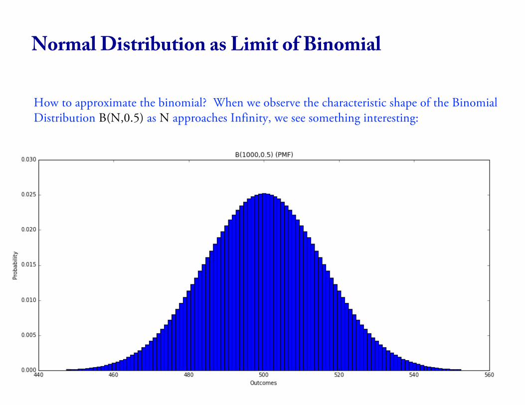
How to approximate the binomial? When we observe the characteristic shape of the Binomial Distribution B(N,0.5) as N approaches Infinity, we see something interesting:

Normal Distribution as Limit of Binomial

22

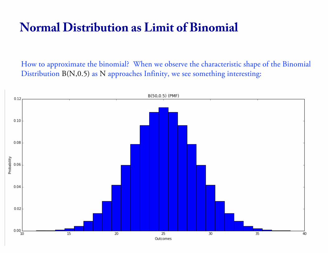
How to approximate the binomial? When we observe the characteristic shape of the Binomial Distribution B(N,0.5) as N approaches Infinity, we see something interesting:

Normal Distribution as Limit of Binomial

23

How to approximate the binomial? When we observe the characteristic shape of the Binomial Distribution B(N,0.5) as N approaches Infinity, we see something interesting:

Normal Distribution as Limit of Binomial

24

How to approximate the binomial? When we observe the characteristic shape of the Binomial Distribution B(N,0.5) as N approaches Infinity, we see something interesting:

Normal Distribution as Limit of Binomial

25

How to approximate the binomial? When we observe the characteristic shape of the Binomial Distribution B(N,0.5) as N approaches Infinity, we see something interesting:

Normal Distribution as Limit of Binomial

26

How to approximate the binomial? When we observe the characteristic shape of the Binomial Distribution B(N,0.5) as N approaches Infinity, we see something interesting:

Normal Distribution as Limit of Binomial

27

How to approximate the binomial? When we observe the characteristic shape of the Binomial Distribution B(N,0.5) as N approaches Infinity, we see something interesting:

Normal Distribution as Limit of Binomial

28

How to approximate the binomial? When we observe the characteristic shape of the Binomial Distribution B(N,0.5) as N approaches Infinity, we see something interesting:

Normal Distribution as Limit of Binomial

29

How to approximate the binomial? When we observe the characteristic shape of the Binomial Distribution B(N,0.5) as N approaches Infinity, we see something interesting:

Normal Distribution as Limit of Binomial

30

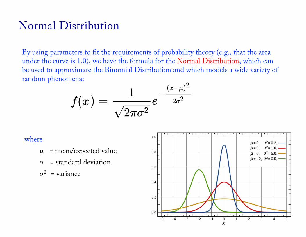
By using parameters to fit the requirements of probability theory (e.g., that the area under the curve is 1.0), we have the formula for the Normal Distribution, which can be used to approximate the Binomial Distribution and which models a wide variety of random phenomena:

where𝜇 = mean/expected value𝜎 = standard deviation𝜎2 = variance

Normal Distribution

The normal distribution, as the limit of B(N,0.5), occurs when a very large number of factors add together to create some random phenomenon.

Example: What is the height of a human being?

Normal Distribution

The normal distribution, as the limit of B(N,0.5), occurs when a very large number of factors add together to create some random phenomenon.

Example: What is the IQ of a human being?

Normal Distribution

The normal distribution, as the limit of B(N,0.5), occurs when a very large number of factors add together to create some random phenomenon.

Example: What is the distribution of measurement errors?

Normal Distribution

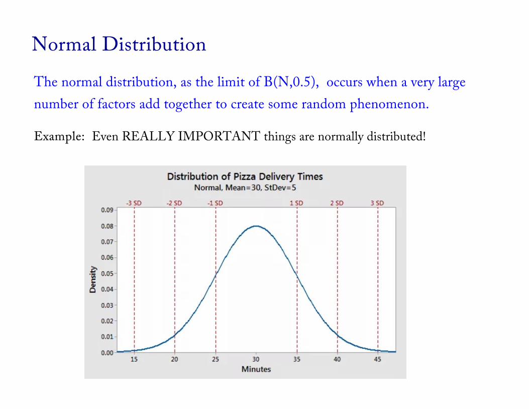
The normal distribution, as the limit of B(N,0.5), occurs when a very large number of factors add together to create some random phenomenon.

Example: Even REALLY IMPORTANT things are normally distributed!

Normal Distribution

35

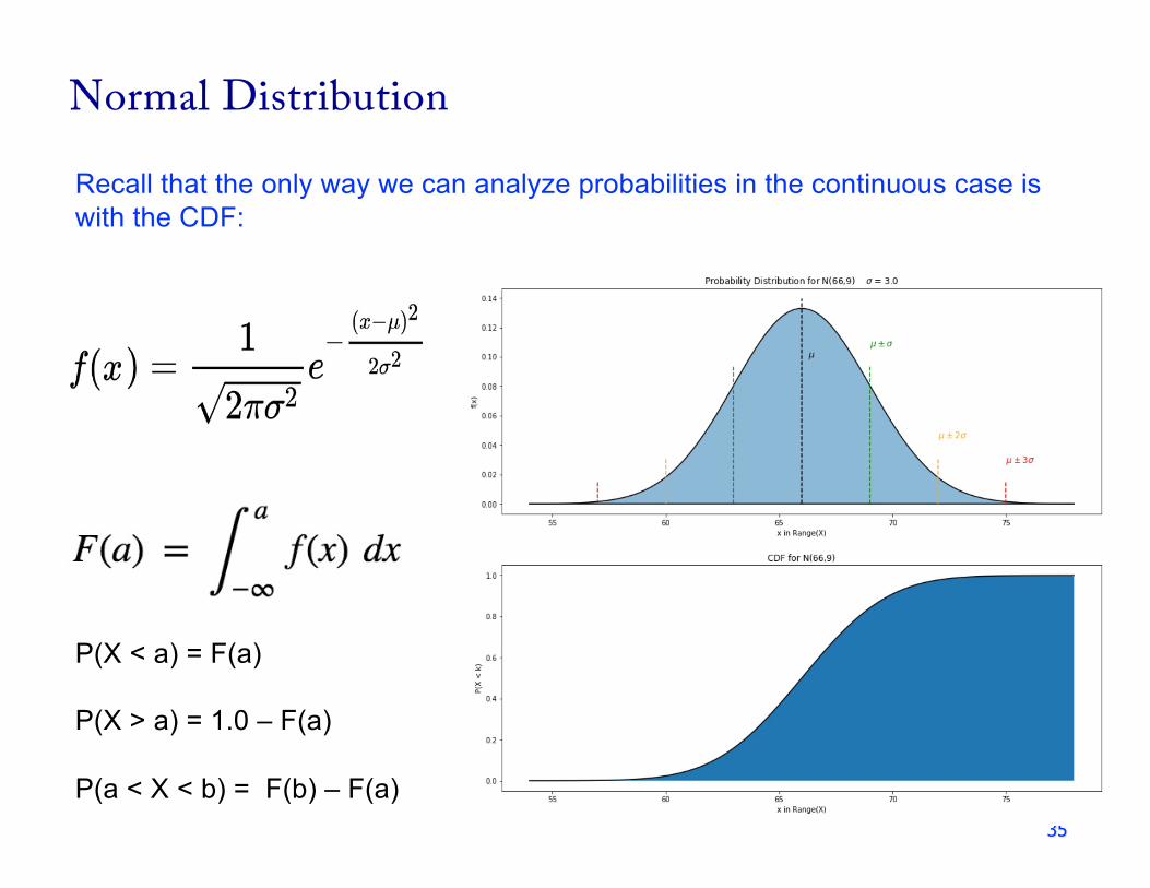
Recall that the only way we can analyze probabilities in the continuous case is with the CDF:

P(X < a) = F(a)

P(X > a) = 1.0 – F(a)

P(a < X < b) = F(b) – F(a)

Normal Distribution

36

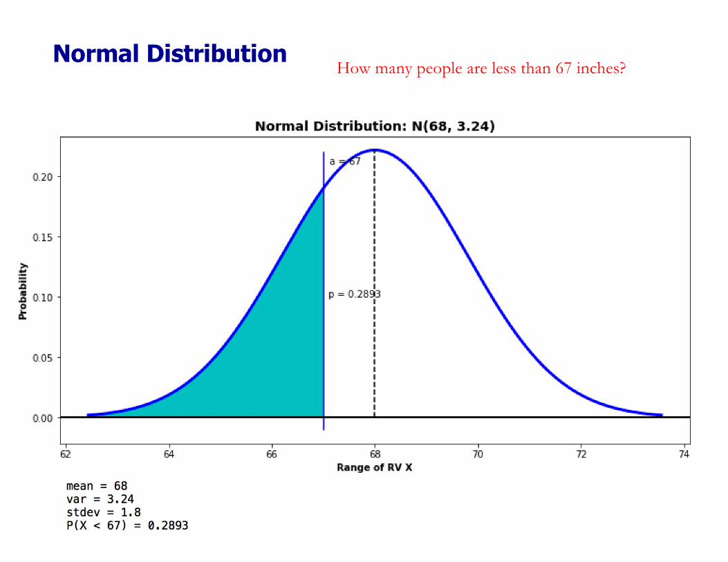
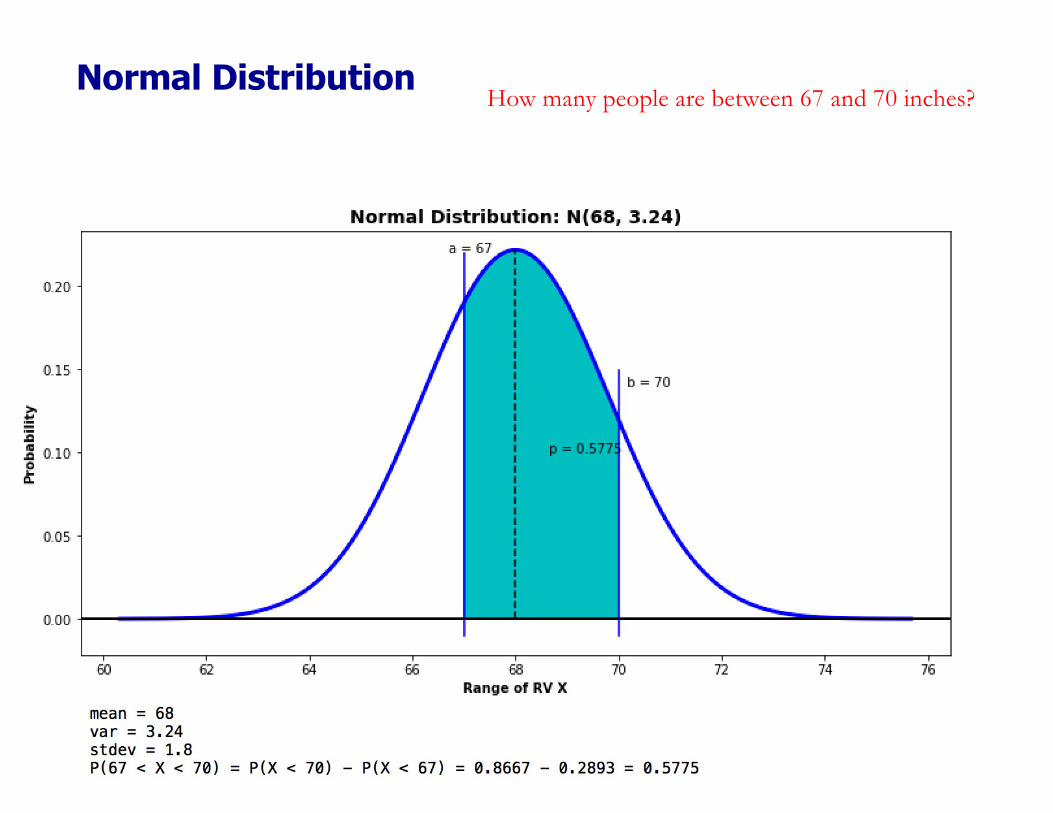
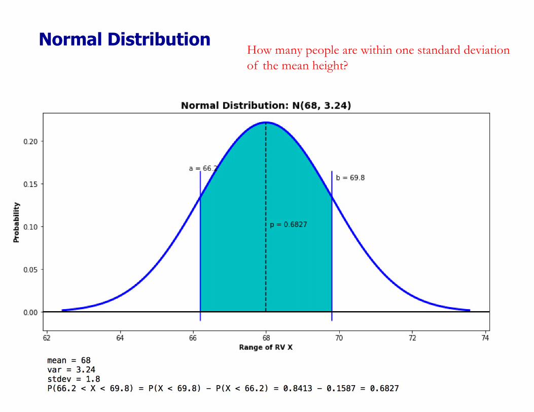
Normal Distribution Suppose heights at BU are distributed normally with a mean of 68 inches and a standard deviation of 1.8 inches.

37

Normal DistributionHow many people are of less than average height?

38

Normal DistributionHow many people are less than 70 inches?

39

Normal DistributionHow many people are less than 67 inches?

40

Normal DistributionHow many people are between 67 and 70 inches?

41

Normal DistributionHow many people are within one standard deviation of the mean height?

42

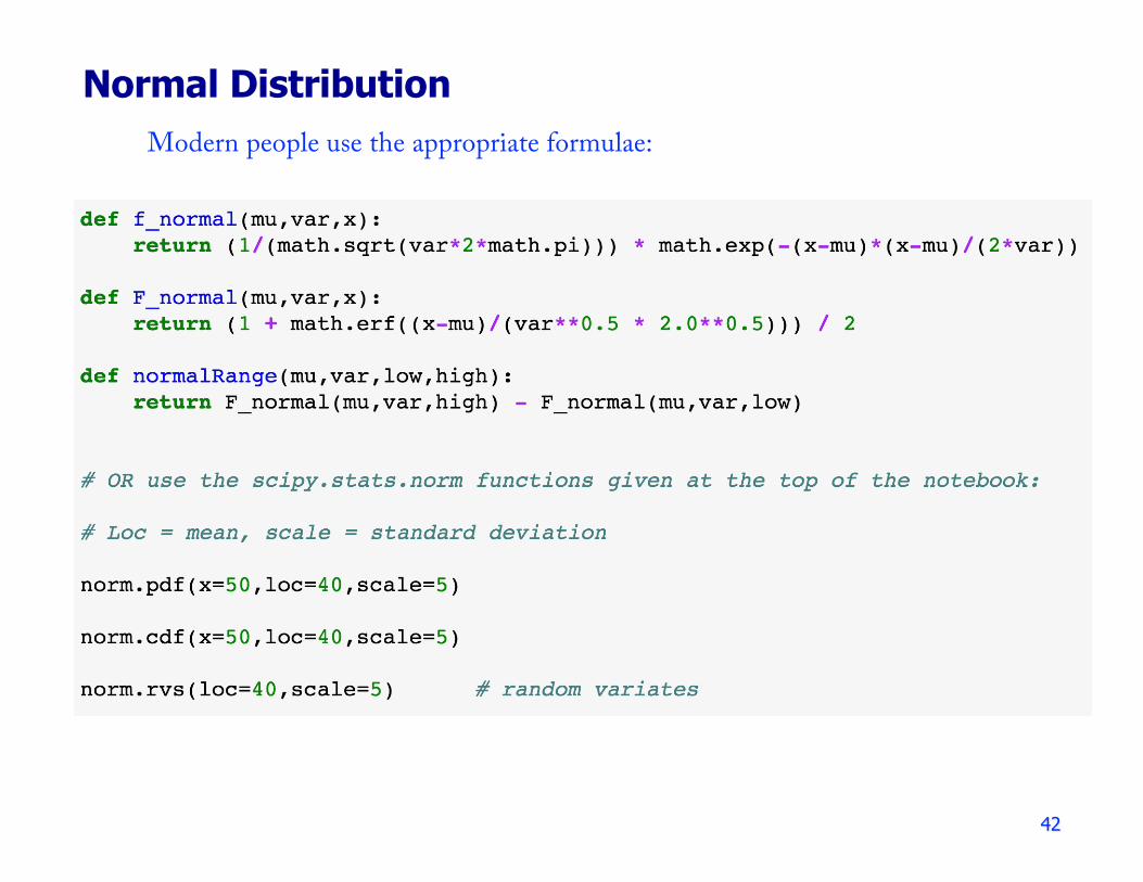
Normal DistributionModern people use the appropriate formulae:

43

Normal DistributionOr a calculator or a web site: