CS 345:Topics in Data Warehousing

Tuesday, October 19, 2004

Review of Thursday’s Class• Indexes

– B-Tree and Hash Indexes– Clustered vs. Non-Clustered– Covering Indexes

• Using Indexes in Query Plans

• Bitmap Indexes– Index intersection plans– Bitmap compression

Outline of Today’s Class

• Bitmap compression with BBC codes– Gaps and Tails– Variable byte-length encoding of lengths– Special handling of lone bits

• Speeding up star joins– Cartesian product of dimensions– Semi-join reduction– Early aggregation

Bitmap Compression

• Compression via run length encoding– Just record number of zeros between adjacent ones– 00000001000010000000000001100000– Store this as “7,4,12,0,5”

• But: Can’t just write 11110011000101– It could be 7,4,12,0,5. (111)(100)(1100)(0)(101) – Or it could be 3,25,8,2,1. (11)(11001)(1000)(10)(1)– Need structured encoding

BBC Codes

• Byte-aligned Bitmap Codes– Proposed by Antoshenkov (1994)– Used in Oracle– We’ll discuss a simplified variation

• Divide bitmap into bytes– Gap bytes are all zeros– Tail bytes contain some ones– A chunk consists of some gap bytes followed by some tail bytes

• Encode chunks– Header byte– Gap length bytes (sometimes)– Verbatim tail bytes (sometimes)

BBC Codes

• Number of gap bytes– 0-6: Gap length stored in header byte– 7-127: One gap-length byte follows header byte– 128-32767: Two gap-length bytes follow header byte

• “Special” tail– Tail of a chunk is special if:

• Tail consists of only 1 byte• The tail byte has only 1 non-zero bit

– Non-special tails are stored verbatim (uncompressed)• Number of tail bytes is stored in header byte

– Special tails are encoded by indicating which bit is set

BBC Codes• Header byte

– Bits 1-3: length of (short) gap• Gaps of length 0-6 don’t require gap length bytes• 111 = gap length > 6

– Bit 4: Is the tail special?– Bits 5-9:

• Number of verbatim bytes (if bit 4=0)• Index of non-zero bit in tail byte (if bit 4 = 1)

• Gap length bytes– Either one or two bytes– Only present if bits 1-3 of header are 111– Gap lengths of 7-127 encoded in single byte– Gap lengths of 128-32767 encoded in 2 bytes

• 1st bit of 1st byte set to 1 to indicate 2-byte case• Verbatim bytes

– 0-15 uncompressed tail bytes– Number is indicated in header

BBC Codes Example• 00000000 00000000 00010000 00000000 00000000 00000000

00000000 00000000 00000000 00000000 00000000 0000000000000000 00000000 00000000 00000000 01000000 00100010

• Consists of two chunks• Chunk 1

– Bytes 1-3– Two gap bytes, one tail byte– Encoding: (010)(1)(0100)– No gap length bytes since gap length < 7– No verbatim bytes since tail is special

• Chunk 2– Bytes 4-18– 13 gap bytes, two tail bytes– Encoding: (111)(0)(0010) 00001101 01000000 00100010– One gap length byte gives gap length = 13– Two verbatim bytes for tail

• 01010100 11100010 00001101 01000000 00100010

Expanding Query Plan Choices

• “Conventional” query planner has limited options for executing star query– Join order: In which order should the dimensions be

joined to the fact?– Join type: Hash join vs. Merge join vs. NLJ– Index selection: Can indexes support the joins?– Grouping strategy: Hashing vs. Sorting for grouping

• We’ll consider extensions to basic join plans– Dimension Cartesian product– Semi-join reduction– Early aggregation

Faster Star Queries

• Consider this scenario– Fact table has 100 million rows– 3 dimension tables, each with 100 rows– Filters select 10 rows from each dimension

• One possible query plan1. Join fact to dimension A

• Produce intermediate result with 10 million rows2. Join result to dimension B

• Produce intermediate result with 1 million rows3. Join result to dimension C

• Produce intermediate result with 100,000 rows4. Perform grouping & aggregation

• Each join is expensive– Intermediate results are quite large

Dimension Cartesian Product• Consider this alternate plan:

– “Join” dimensions A and B• Result is Cartesian product of all combinations• Result has 100 rows (10 A rows * 10 B rows)

– “Join” result to dimension C• Another Cartesian product • 1000 rows (10 A rows * 10 B rows * 10 C rows)

– Join result to fact table• Produce intermediate result with 100,000 rows

– Perform grouping and aggregation• Computing Cartesian product is cheap

– Few rows in dimension tables• Only one expensive join rather than three• Approach breaks down with:

– Too many dimensions– Too many rows in each dimension satisfy filters

Dimension Cartesian Product

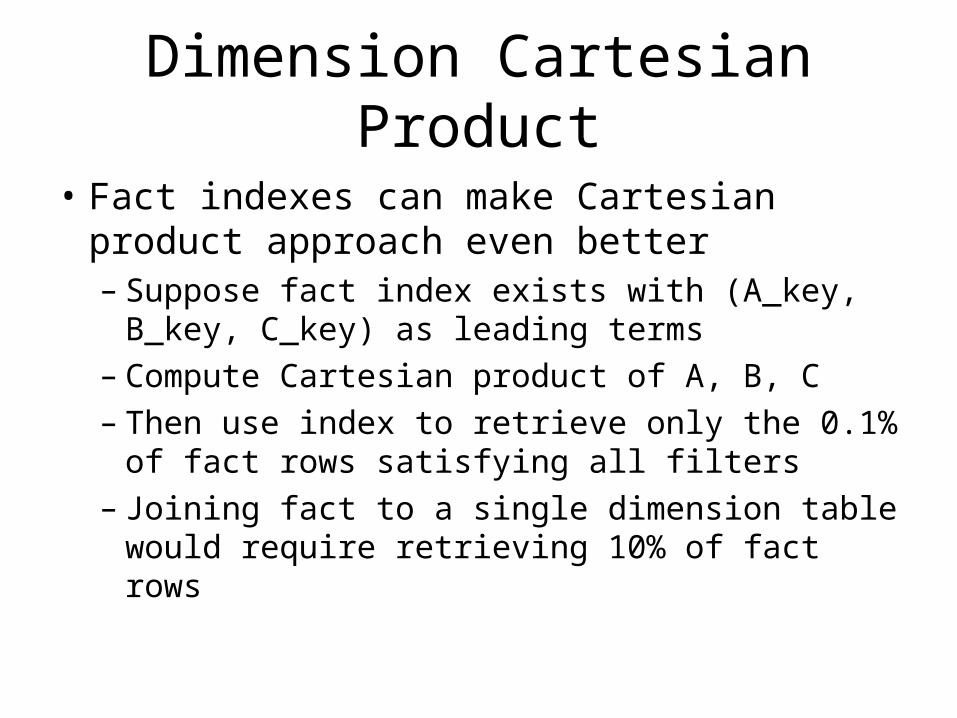
• Fact indexes can make Cartesian product approach even better– Suppose fact index exists with (A_key, B_key,

C_key) as leading terms– Compute Cartesian product of A, B, C– Then use index to retrieve only the 0.1% of

fact rows satisfying all filters– Joining fact to a single dimension table would

require retrieving 10% of fact rows

Cartesian Product Pros & Cons

• Benefits of dimension Cartesian product– Fewer joins involve fact table or its derivatives– Leverage filtering power of multi-column fact indexes

with composite keys

• Drawbacks of dimension Cartesian product– Cartesian product result can be very large– More stringent requirements on fact indexes

• Fact index must include all dimensions from Cartesian product to be useful

• Dimension-at-a-time join plans can use thin fact index for initial join

Semi-Join Reduction

• Query plans involving semi-joins are common in distributed databases

• Semi-join of A with B (A B)– All rows in A that join with at least 1 row from B– Discard non-joining rows from A– Attributes from B are not included in the result

• Semi-join of B with A (B A)– All rows in B that join with at least 1 row from A– A B != B A

• Identity: A B = A (B A)

Semi-Join Reduction• To compute join of A and B on A.C1 = B.C2:

– Server 1 sends C1 values from A to Server 2– Server 2 computes semi-join of B with A– Server 2 sends joining B tuples to Server 1– Server 1 computes join of A and B

• Better sending simply sending entire B when:– Not too many B rows join with qualifying A rows

A B

A.C1

B

Server 1 Server 2

Semi-Join Reduction for Data Warehouses

• Goal is to save disk I/O rather than network I/O– Dimension table is “Server 1”– Fact table is “Server 2”– Fact table has single-column index on each foreign key column

• Query plan goes as follows:– For each dimension table:

• Determine keys of all rows that satisfy filters on that dimension• Use single-column fact index to look up RIDs of all fact rows with

those dimension keys– Merge RID lists corresponding to each dimension– Retrieve qualifying fact rows– Join fact rows back to full dimension tables to learn grouping

attributes– Perform grouping and aggregation

Semi-Join Reduction

• Semi-join query plan reduces size of intermediate results that must be joined– Intermediate results can be sorted, hashed

more efficiently

Dim Fact

Dim Keys

Fact

Server 1 Server 2

Semi-Join Reduction

Dimension Table

Apply filters to eliminatenon-qualifying rows

Generate list of dimension keys

1 Fact Index

Dim.Keys

2

Semi-joinfact index anddimension keys

=

3

Intersect fact RID lists

Semi-Join Reduction4

Lookup fact rowsbased on RIDs

Fact Table

FactRIDs

5

Join back to dimensionsto bring in grouping attributes

Dimension Table

Fact Rows

Semi-Join Reduction Pros &Cons

• Benefits of semi-join reduction– Makes use of thin (1-column) fact indexes– Only relevant fact rows need be retrieved

• Apply all filters before retrieving any fact rows

• Drawbacks of semi-join reduction– Incur overhead of index intersection– Looking up fact rows from RIDs can be expensive

• Random I/O• Only good when number of qualifying fact rows is small

– Potential to access same dimension twice• Initially when generating dimension key list• Later when joining back to retrieve grouping columns

Early Aggregation• Query plans we’ve considered do joins first, then grouping and

aggregation• Sometimes “group by” can be handled in two phases

– Perform partial aggregation early as a data reduction technique– Finish up the aggregation after completing all joins

• Example:– SELECT Store.District, SUM(DollarSales)

FROM Sales, Store, DateWHERE Sales.Store_key = Store.Store_keyAND Sales.Date_key = Date.Date_keyAND Date.Year = 2003GROUP BY Store.District

– Lots of Sales rows, but fewer distinct (Store, Date) combinations• Early aggregation plan:

1. Group Sales by (Store, Date) & compute SUM(DollarSales)2. Join result with Date dimension, filtered based on Year3. Join result with Store dimension4. Group by District & compute SUM(DollarSales)

Compare with Conventional Plan

• Conventional plan– Join Sales and Date,

filtering based on Year• Result has 36 million rows

– Join result with Product• Result has 36 million rows

– Group by District & compute aggregate

• Early aggregation plan– Group Sales by (Date, Product)

& compute aggregate• Result has 100,000 rows

– Join result with Date• Result has 36,500 rows

– Join result with District• Result has 36,500 rows

– Group by District & compute aggregate

• Assumptions– Sales fact has 100 million rows

– Store dimension has 100 rows

– Date dimension has 1000 rows (365 in 2003)

Early Aggregation Pros & Cons

• Benefits of early aggregation– Initial aggregation can be fast with appropriate covering index

• Leverage fact index on (Date, Store, DollarSales)

– Result of early aggregation significantly smaller than fact table• Fewer rows• Fewer columns

– Joins to dimension tables are cheaper• Because intermediate result is much smaller than fact table

• Drawbacks of early aggregation– Can’t take advantage of data reduction due to filters

• Prefer joins with highly selective filters (Date.Day = 'October 20, 2004') before early aggregation

– Two aggregation steps instead of one• Adds additional overhead

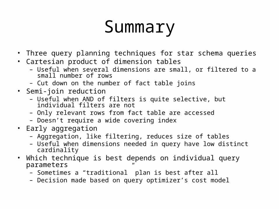
Summary• Three query planning techniques for star schema queries• Cartesian product of dimension tables

– Useful when several dimensions are small, or filtered to a small number of rows

– Cut down on the number of fact table joins• Semi-join reduction

– Useful when AND of filters is quite selective, but individual filters are not– Only relevant rows from fact table are accessed– Doesn’t require a wide covering index

• Early aggregation– Aggregation, like filtering, reduces size of tables– Useful when dimensions needed in query have low distinct cardinality

• Which technique is best depends on individual query parameters– Sometimes a “traditional” plan is best after all– Decision made based on query optimizer’s cost model