CS 376Introduction to Computer Graphics

03 / 30 / 2007

Instructor: Michael Eckmann

Michael Eckmann - Skidmore College - CS 376 - Spring 2007

Today’s Topics• Questions?

• Illumination modeling– we already covered

• ambient term• point light source

– with diffusely reflecting surfaces– with distance attenuation of light

– let's continue with• specularly reflecting surfaces• colored light• colored surfaces• multiple point light sources

– Transparent/translucent surfaces

• Shading– flat

Michael Eckmann - Skidmore College - CS 376 - Spring 2007

Illumination• Specular reflection as stated before is a property of a surface

where light is reflected in unequal intensities at different

directions.

• A perfect mirror reflects light in only one direction. Less

perfectly shiny surfaces reflect light more in one particular

direction than other directions.

• Either way, consider the angle the light and the surface

normal makes. The direction that the most intense light is

reflected is at an angle which is equal to that angle but on the

other side of the surface normal.

• The next slide has a diagram for specular reflection.

Illumination• L is a vector in the direction of the light source. N is the surface normal.

R is the vector which is in the direction of the maximum specular

reflection. V is the vector in the direction toward the viewer.

• The angle between L and N is the same as the angle between N and R.

• The angle phi, between R and V affects how much light is reflected in

V's direction.

• If the surface was a perfect mirror, then light is only reflected along R. If

the surface is shiny, but not perfect, light is reflected mostly in R's

direction but decreases reflection as we go in directions at angles away

from R.

• An illumination model that takes into account non perfect specular

reflections is the Phong model.

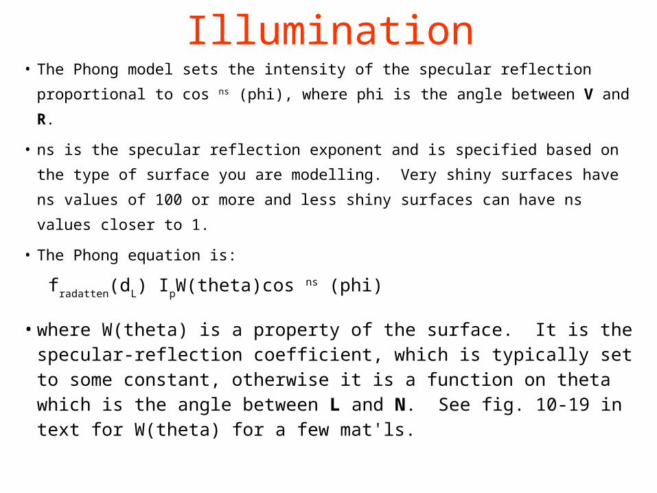
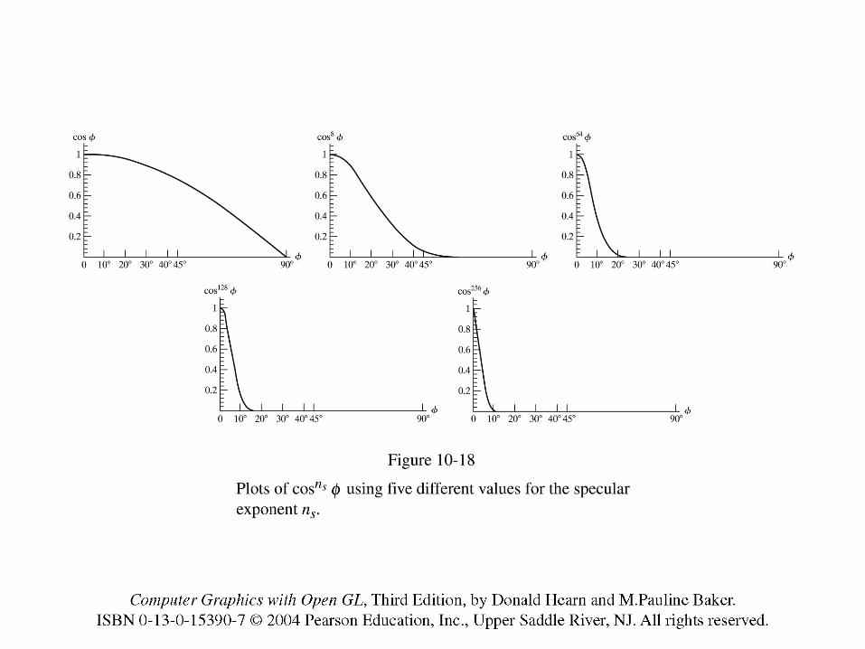
Illumination• The Phong model sets the intensity of the specular reflection proportional

to cos ns (phi), where phi is the angle between V and R.

• ns is the specular reflection exponent and is specified based on the type

of surface you are modelling. Very shiny surfaces have ns values of 100

or more and less shiny surfaces can have ns values closer to 1.

• The Phong equation is:

fradatten

(dL) I

pW(theta)cos ns (phi)

• where W(theta) is a property of the surface. It is the specular-

reflection coefficient, which is typically set to some constant,

otherwise it is a function on theta which is the angle between

L and N. See fig. 10-19 in text for W(theta) for a few mat'ls.

Illumination

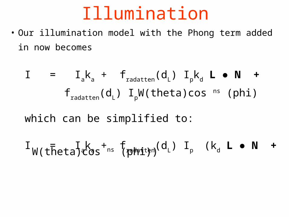
Illumination• Our illumination model with the Phong term added in now becomes

I = Iak

a + f

radatten(d

L) I

pk

d L ● N +

fradatten

(dL) I

pW(theta)cos ns (phi)

which can be simplified to:

I = Iak

a + f

radatten(d

L) I

p (k

d L ● N + W(theta)cos ns (phi))

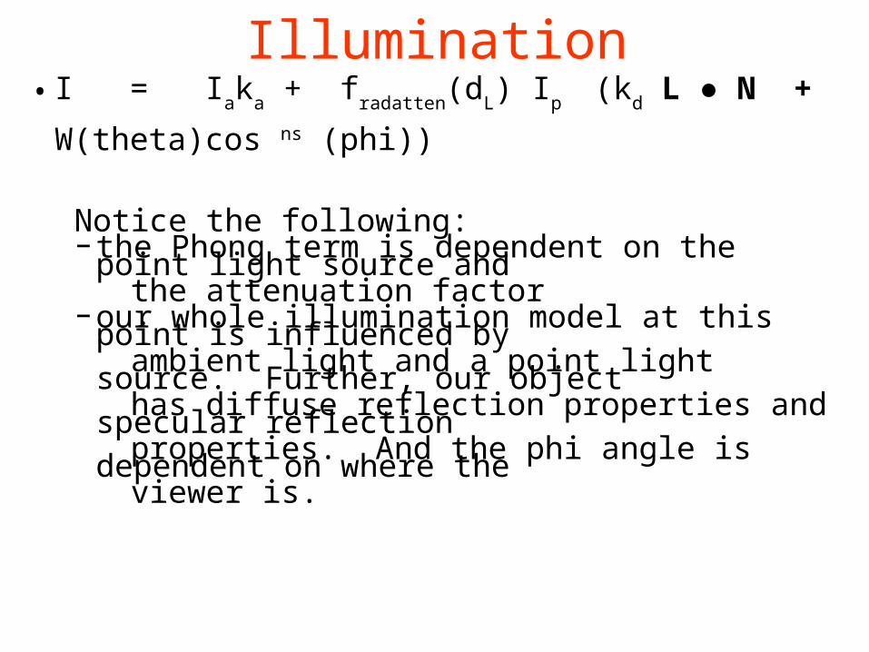
Illumination• I = I

ak

a + f

radatten(d

L) I

p (k

d L ● N + W(theta)cos ns (phi))

Notice the following:– the Phong term is dependent on the point light source and the attenuation factor– our whole illumination model at this point is influenced by ambient light and a point light source. Further, our object has diffuse reflection properties and specular reflection properties. And the phi angle is dependent on where the viewer is.

Illumination• If we have more than one point light source (which is white

light), then we sum up over all the light sources i:

I = Iak

a + Sum

all i [f

radatten(d

L) I

pi (k

d L ● N + W(theta)cos ns (phi))]

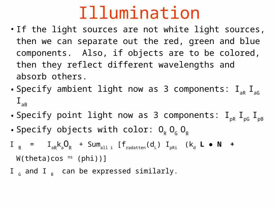
Illumination• If the light sources are not white light sources, then we can

separate out the red, green and blue components. Also, if

objects are to be colored, then they reflect different

wavelengths and absorb others.

• Specify ambient light now as 3 components: IaR

IaG

IaB

• Specify point light now as 3 components: IpR

IpG

IpB

• Specify objects with color: OR

OG

OB

I R = I

aRk

aO

R + Sum

all i [f

radatten(d

L) I

pRi (k

d L ● N + W(theta)cos ns (phi))]

I G and I

B can be expressed similarly.

Illumination• We typically want our Intensities to be in the range 0 to 1. With many

light sources that are specified as too intense, computed intensities of

objects can easily be too large (> 1).

• We can normalize the range of calculated intensities into the range 0 to 1.

• Or we can specify our light source intensities better and if any

calculations go over 1, then clip them to intensity 1.

Directional light source• The light sources that we have discussed so far were point light sources

which radiated light in all directions. Many real lights in the world do

not have this property. Instead, lights can be directional.

• A directional light source can be described as having – a position– a directional vector – an angular limit from that vector– a color

• The vector will be the axis in a cone shaped volume. This volume is the

only part of space that will be illuminated by this light. Anything outside

the cone will not be illuminated by this light.

• See diagram next slide.

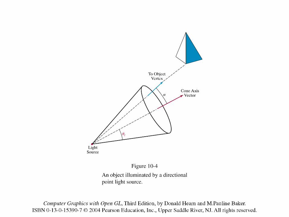
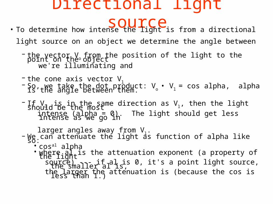
Directional light source• To determine how intense the light is from a directional light source on

an object we determine the angle between

– the vector Vo from the position of the light to the point on the object

we're illuminating and

– the cone axis vector Vl– So, we take the dot product: V

o • V

l = cos alpha, alpha is the angle

between them.

– If Vo is in the same direction as V

l, then the light should be the most

intense (alpha = 0). The light should get less intense as we go in

larger angles away from Vl.

– We can attenuate the light as function of alpha like so: • cosal alpha• where al is the attenuation exponent (a property of the light

source) --- if al is 0, it's a point light source, the smaller al is,the larger the attenuation is (because the cos is less than 1.)

Transparent/Translucent surfaces• Transparent, opaque, translucent

– Transparent refers to the quality of a surface that we can “see through”. Opaque surfaces, we cannot see through.

– some transparent objects are translucent --- light is transmitted diffusely in all directions through the material

– translucent materials make the object viewed through them blurry

Transparent/Translucent surfaces• Terminology

• index of refraction of a material

– is defined to be the ratio of the speed of light in a vacuum

to the speed of light in the material.

• Snell's Law is a relationship between angle of incidence and

refraction and indices of refraction.

Transparent/Translucent surfaces• To determine the direction of the refracted ray, the angle ( theta

r )

off of -N, we need to know several things

– the direction of the incoming ray, the angle ( thetai ) of incidence

– the index of refraction (etai ) of the material the ray is coming from

– the index of refraction (etar ) of the material the ray is entering

Transparent/Translucent surfaces• Snell's law states that

sin ( thetar ) eta

i -------------- = -----sin ( theta

i ) eta

r

• which can be written as:

sin ( thetar ) = ((eta

i ) / (eta

r )) * sin ( theta

i )

Transparent/Translucent surfaces• Assuming all of our vectors are unit vectors, using Snell's law, according

to our textbook we can compute the unit refracted ray, T, to be

T = (((etai ) / (eta

r )) cos ( theta

r ) – cos ( theta

r )) N – ((eta

i ) / (eta

r ))L

• See page 578 in our text.

• This assumes L is in the direction shown in the diagram of figure 10-30.

• Verifying that the equation above is correct is left as an exercise to the

reader. It may appear on a hw assignment.

Transparent/Translucent surfaces• Table 10-1 on page 578 in our text shows average indices of refraction

for common materials, such as

• Vacuum (1.0), Ordinary Crown Glass (1.52), Heavy Crown Glass (1.61), Ordinary Flint Glass (1.61), Heavy Flint Glass (1.92), Rock Salt (1.55), Quartz (1.54), Water (1.33), Ice (1.31)

• Different frequencies of light travel at different speeds through the same material. Therefore, each frequency has its own index of refraction. The indices of refraction above are averages.

Surface Rendering• Now that we have an illumination model built, we can use it in different

ways to do surface rendering aka shading.

Shading Models• Constant shading (aka flat shading, aka faceted shading) is the simplest

shading model.

• It is accurate when a polygon face of an object is not approximating a

curved surface, all light sources are far and the viewer is far away from

the object. Far meaning sufficiently far enough away that N • L and R •

V are constant across the polygon.

• If we use constant shading but the light and viewer are not sufficiently far

enough away then we need to choose a value for each of the dot products

and apply it to the whole surface. This calculation is usually done on the

centroid of the polygon.

• Advantages: fast & simple

• Disadvantages: inaccurate shading if the assumptions are not met.

Shading Models• Interpolated shading model

– Assume we're shading a polygon. The shading is interpolated

linearly. That is, we calculate a value at two points and interpolate

between them to get the value at the points in between --- this saves

lots of computation (over computing at each position) and results in a

visual improvement over flat shading.

– This technique was created for triangles e.g. compute the color at the

three vertices and interpolate to get the edge colors and then

interpolate across the triangle's surface from edge to edge to get the

interior colors.

– Gouraud shading is an interpolation technique that is generalized to

arbitrary polygons. Phong shading is another interpolation technique

but doesn't interpolate intensities.

Shading Models• Gouraud shading (aka Gouraud Surface Rendering) is a form of

interpolated shading.

– How to calculate the intensity at the vertices?

• we have normal vectors to all polygons so, consider all the

polygons that meet at that vertex. Drawing on the board.

• Suppose for example, n polygons all meet at one vertex. We

want to approximate the normal of the actual surface at the

vertex. We have the normals to all n polygons that meet there.

So, to approximate the normal to the vertex we take the average

of all n polygon normals.

• What good is knowing the normal at the vertex? Why do we

want to know that?

Shading Models• Gouraud shading.

– What good is knowing the normal at the vertex? Why do we want to

know that?

• so we can calculate the intensity at that vertex from the

illumination equations.

– Calculate the intensity at each vertex using the normal we estimate

there.

– Then linearly interpolate the intensity along the edges between the

vertices.

– Then linearly interpolate the intensity along a scan line for the

intensities of interior points of the polygon.

– Example on the board.

Shading Models• Advantages: easy to implement if already doing a scan line algorithm.

• Disadvantages:

– Unrealistic if the polygon doesn't accurately represent the object.

This is typical with polygon meshes representing curved surfaces.

– Mach banding problem

• when there are discontinuities in intensities at polygon edges, we

can sometimes get this unfortunate effect.

• let's see an example.

– The shading of the polygon depends on its orientation. If it rotates,

we will see an unwanted effect due to the interpolation along a

scanline. Example on board.

– Specular reflection is also averaged over polygons and therefore

doesn't accurately show these reflections.

Shading Models• Phong shading (aka Phong Surface Rendering).

– Assume we are using a polygon mesh to estimate a surface.

– Compute the normals at the vertices like we did for Gouraud.

– Then instead of computing the intensity (color) at the vertices and

interpolating the intensities, we interpolate the normals.

– So, given normals at two points of a polygon, we interpolate over the

surface to estimate the normals between the two points.

– Example picture on the board.

– Then we have to apply the illumination equation at all the points in

between to compute intensity. We didn't have to do this for Gouraud.

– Problems arise since the interpolation is done in the 3d world space

and the pixel intensities are in the image space.

Shading Models• Recap

– Flat Shading

– Gouraud Shading --- interpolates intensities

– Phong Shading --- interpolates normal vectors (before calculating

illumination.)

– For these three methods, as speed/efficiency decreases, realism

increases (as you'd expect.)

– They all have the problem of silhouetting. Edges of polygons on the

visual edge of an object are apparent.

– Let's see examples of Gouraud and Phong shading.