cs 416 artificial intelligence lecture 22 statistical learning chapter 20.5 lecture 22 statistical...
TRANSCRIPT
CS 416Artificial Intelligence
Lecture 22Lecture 22
Statistical LearningStatistical Learning
Chapter 20.5Chapter 20.5
Lecture 22Lecture 22
Statistical LearningStatistical Learning
Chapter 20.5Chapter 20.5
Perceptrons
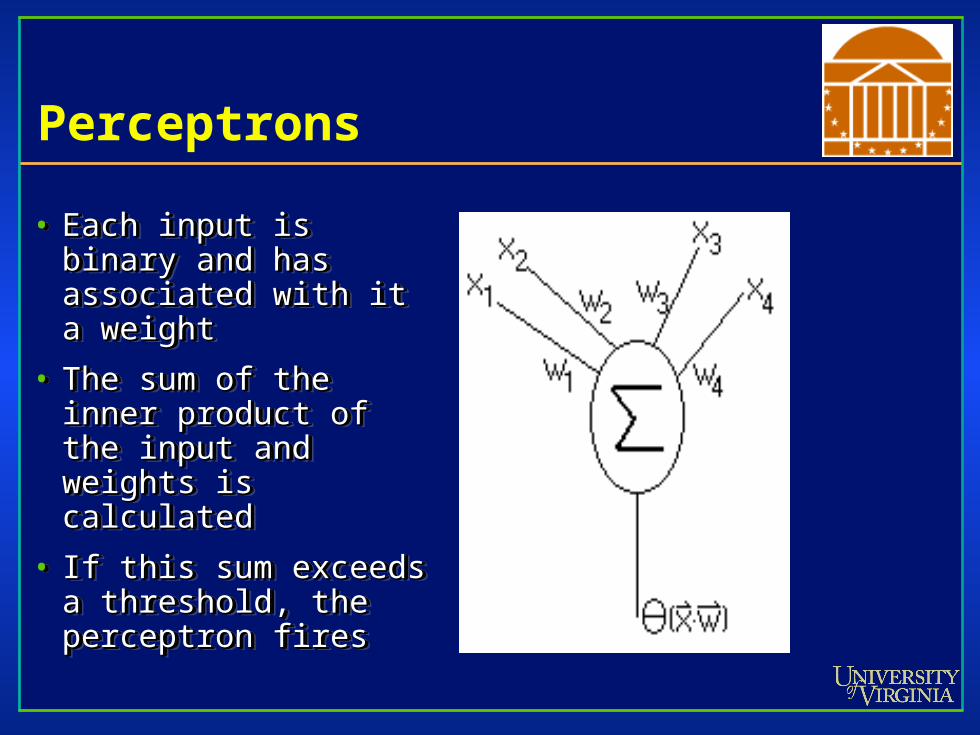
• Each input is binary and Each input is binary and has associated with it a has associated with it a weightweight
• The sum of the inner The sum of the inner product of the input and product of the input and weights is calculatedweights is calculated
• If this sum exceeds a If this sum exceeds a threshold, the perceptron threshold, the perceptron firesfires
Perceptrons are linear classifiers
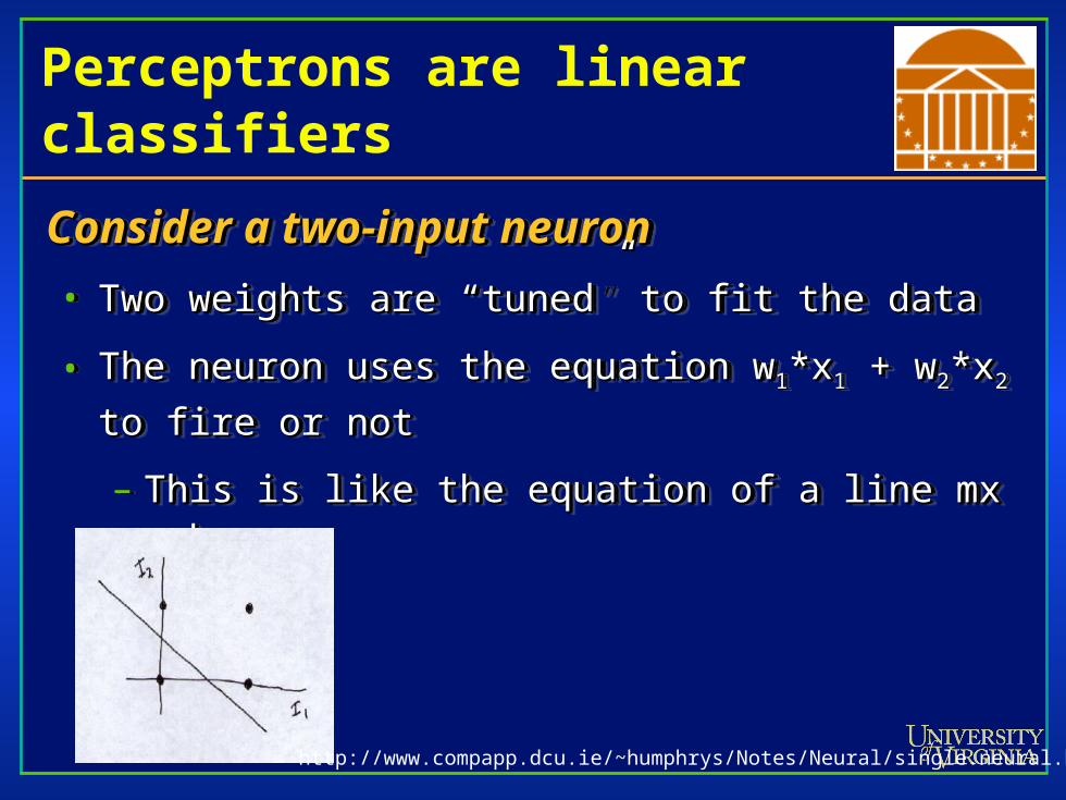
Consider a two-input neuronConsider a two-input neuron
• Two weights are “tuned” to fit the dataTwo weights are “tuned” to fit the data
• The neuron uses the equation wThe neuron uses the equation w11*x*x11 + w + w22*x*x22 to fire or to fire or
notnot
– This is like the equation of a line mx + b - yThis is like the equation of a line mx + b - y
http://www.compapp.dcu.ie/~humphrys/Notes/Neural/single.neural.html
Linearly separable
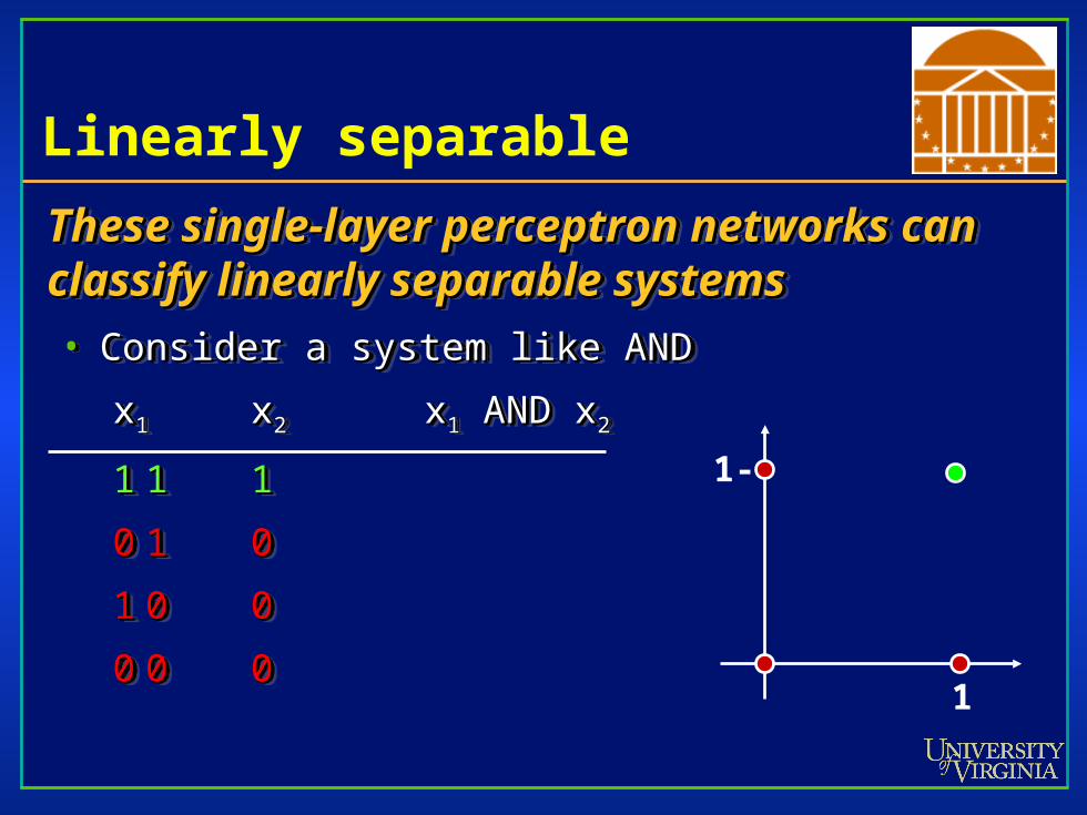
These single-layer perceptron networks can These single-layer perceptron networks can classify linearly separable systemsclassify linearly separable systems• Consider a system like ANDConsider a system like AND
xx1 1 xx22 x x11 AND x AND x22
11 11 11
00 11 00
11 00 00
00 00 00
These single-layer perceptron networks can These single-layer perceptron networks can classify linearly separable systemsclassify linearly separable systems• Consider a system like ANDConsider a system like AND
xx1 1 xx22 x x11 AND x AND x22
11 11 11
00 11 00
11 00 00
00 00 00
1-
1
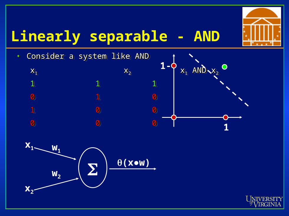
Linearly separable - AND• Consider a system like ANDConsider a system like AND
xx1 1 xx22 x x11 AND x AND x22
11 11 11
00 11 00
11 00 00
00 00 00
• Consider a system like ANDConsider a system like AND
xx1 1 xx22 x x11 AND x AND x22
11 11 11
00 11 00
11 00 00
00 00 00
1-
1
x1
x2
w1
w2
(x●w)
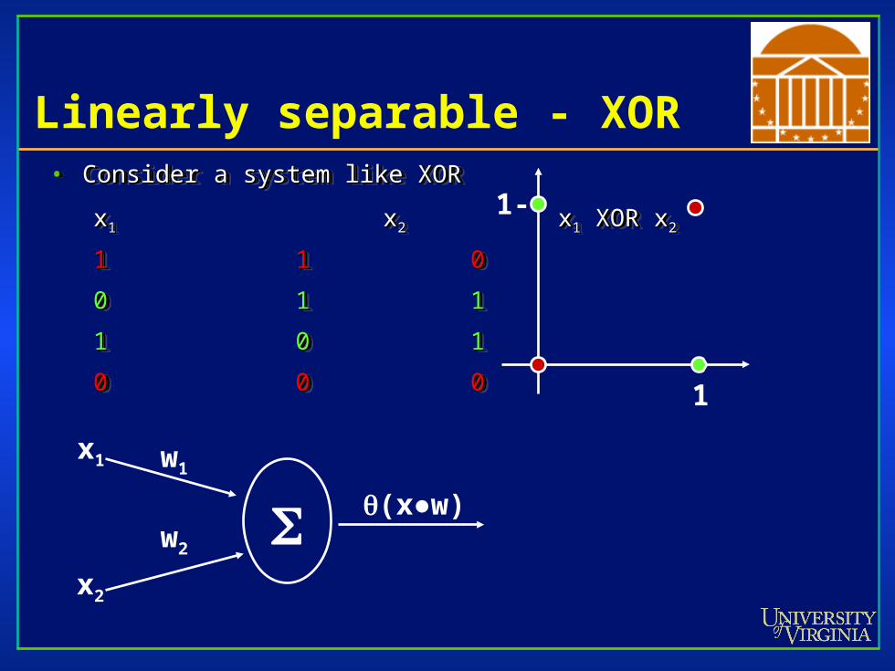
Linearly separable - XOR• Consider a system like XORConsider a system like XOR
xx1 1 xx22 x x11 XOR x XOR x22
11 11 00
00 11 11
11 00 11
00 00 00
• Consider a system like XORConsider a system like XOR
xx1 1 xx22 x x11 XOR x XOR x22
11 11 00
00 11 11
11 00 11
00 00 00
1-
1
x1
x2
w1
w2
(x●w)

Linearly separable - XOR
IMPOSSIBLE!
2nd Class Exercise
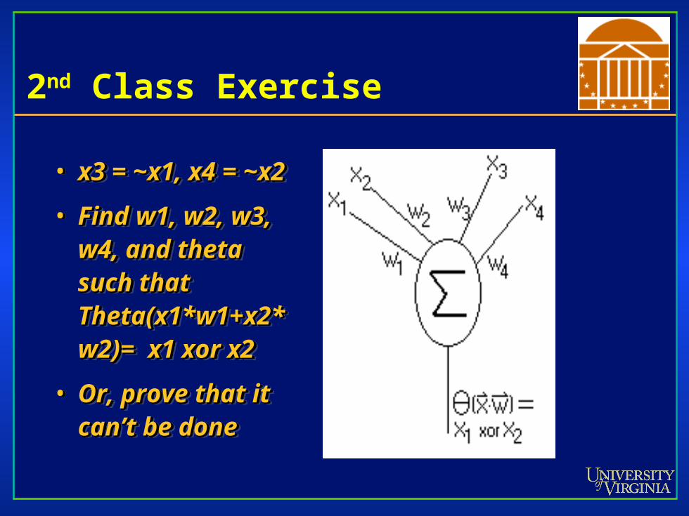
• x3 = ~x1, x4 = ~x2x3 = ~x1, x4 = ~x2
• Find w1, w2, w3, Find w1, w2, w3, w4, and theta w4, and theta such that such that Theta(x1*w1+x2*Theta(x1*w1+x2*w2)= x1 xor x2w2)= x1 xor x2
• Or, prove that it Or, prove that it can’t be donecan’t be done
• x3 = ~x1, x4 = ~x2x3 = ~x1, x4 = ~x2
• Find w1, w2, w3, Find w1, w2, w3, w4, and theta w4, and theta such that such that Theta(x1*w1+x2*Theta(x1*w1+x2*w2)= x1 xor x2w2)= x1 xor x2
• Or, prove that it Or, prove that it can’t be donecan’t be done
3rd Class Exercise
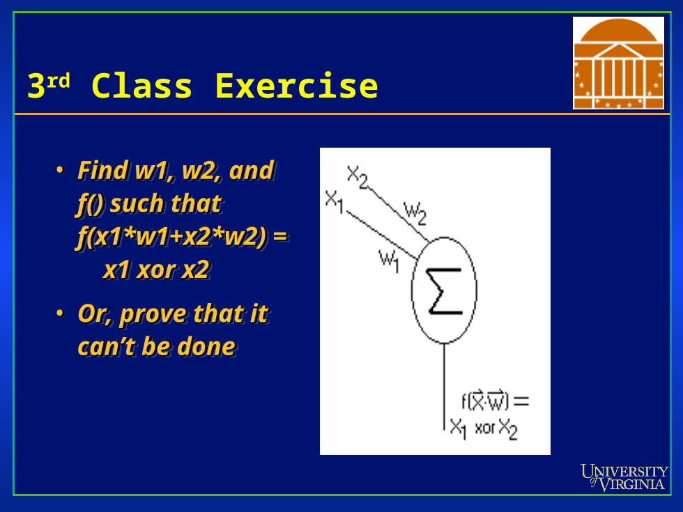
• Find w1, w2, and Find w1, w2, and f() such that f() such that f(x1*w1+x2*w2) = f(x1*w1+x2*w2) = x1 xor x2 x1 xor x2
• Or, prove that it Or, prove that it can’t be donecan’t be done
• Find w1, w2, and Find w1, w2, and f() such that f() such that f(x1*w1+x2*w2) = f(x1*w1+x2*w2) = x1 xor x2 x1 xor x2
• Or, prove that it Or, prove that it can’t be donecan’t be done
Limitations of Perceptrons
• Minsky & Papert published (1969) Minsky & Papert published (1969) “Perceptrons” stressing the limitations of “Perceptrons” stressing the limitations of perceptronsperceptrons
• Single-layer perceptrons cannot solve Single-layer perceptrons cannot solve problems that are linearly inseparable (e.g., problems that are linearly inseparable (e.g., xor)xor)
• Most interesting problems are linearly Most interesting problems are linearly inseparableinseparable
• Kills funding for neural nets for 12-15 yearsKills funding for neural nets for 12-15 years
A brief aside about Marvin Minsky
• Attended Bronx H.S. of ScienceAttended Bronx H.S. of Science
• Served in U.S. Navy during WW IIServed in U.S. Navy during WW II
• B.A. Harvard and Ph.D. PrincetonB.A. Harvard and Ph.D. Princeton
• MIT faculty since 1958MIT faculty since 1958
• First graphical head-mounted display (1963)First graphical head-mounted display (1963)
• Co-inventor of Logo (1968)Co-inventor of Logo (1968)
• Nearly killed during 2001: A Space Odyssey but survived to write Nearly killed during 2001: A Space Odyssey but survived to write paper critical of neural networkspaper critical of neural networks
• Turing Award 1970Turing Award 1970
From wikipedia.org
Single-layer networks for classification
• Single output with 0.5 as dividing line for binary Single output with 0.5 as dividing line for binary classificationclassification
• Single output with n-1 dividing lines for n-ary Single output with n-1 dividing lines for n-ary classificationclassification
• n outputs with 0.5 dividing line for n-ary classificationn outputs with 0.5 dividing line for n-ary classification
Recent History of Neural Nets
• 1969 Minsky & Papert “kill” neural nets1969 Minsky & Papert “kill” neural nets
• 1974 Werbos describes back-1974 Werbos describes back-propagationpropagation
• 1982 Hopfield reinvigorates neural nets1982 Hopfield reinvigorates neural nets
• 1986 Parallel Distributed Processing1986 Parallel Distributed Processing
Multi-layered Perceptrons
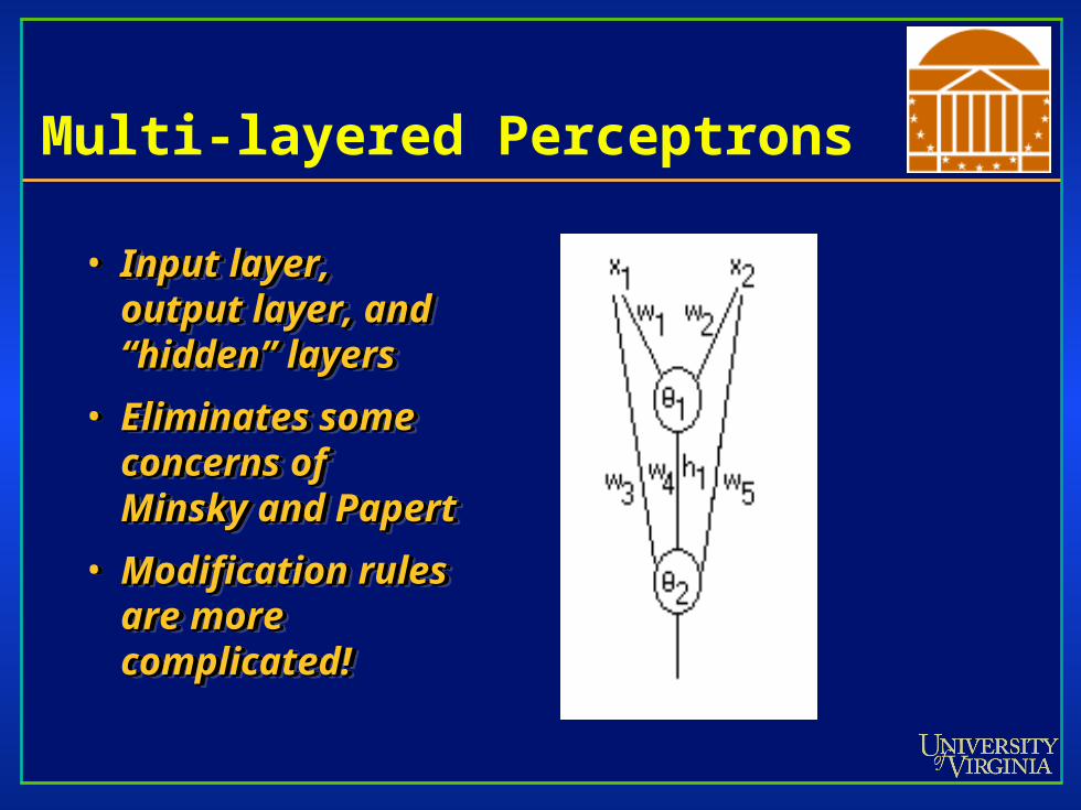
• Input layer, output Input layer, output layer, and layer, and “hidden” layers“hidden” layers
• Eliminates some Eliminates some concerns of concerns of Minsky and PapertMinsky and Papert
• Modification rules Modification rules are more are more complicated!complicated!
• Input layer, output Input layer, output layer, and layer, and “hidden” layers“hidden” layers
• Eliminates some Eliminates some concerns of concerns of Minsky and PapertMinsky and Papert
• Modification rules Modification rules are more are more complicated!complicated!
Why are modification rules more complicated?
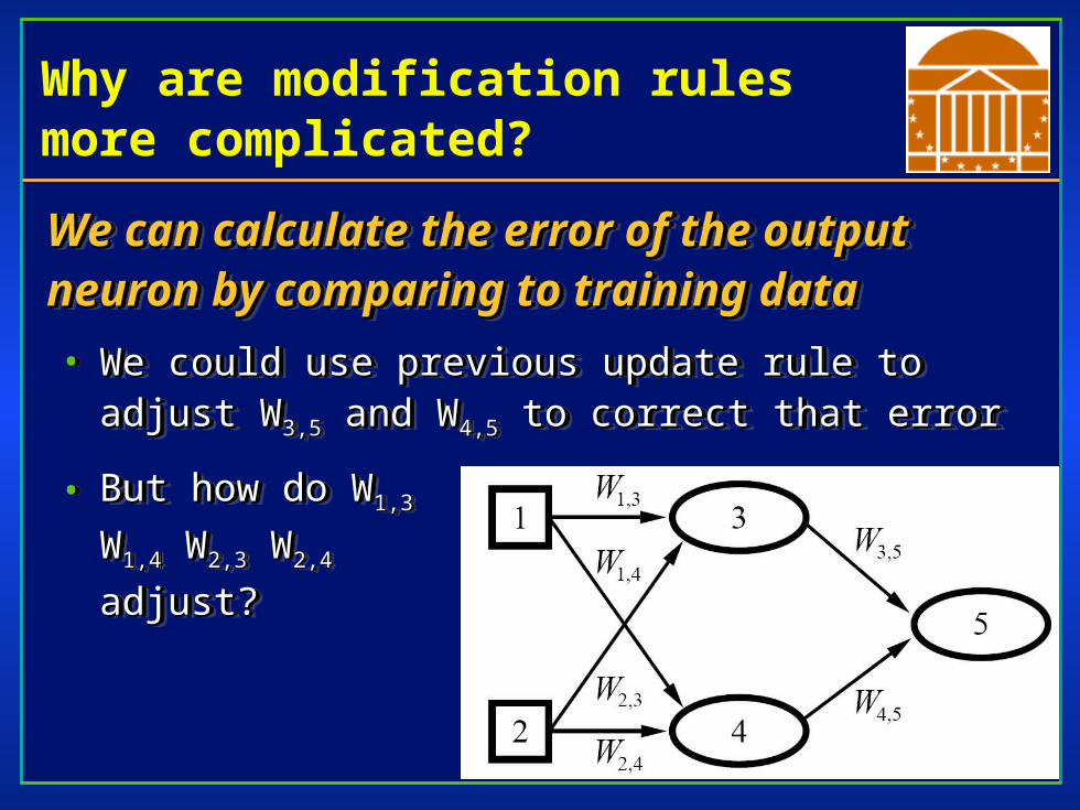
We can calculate the error of the output We can calculate the error of the output neuron by comparing to training dataneuron by comparing to training data
• We could use previous update rule to adjust WWe could use previous update rule to adjust W3,53,5 and and
WW4,54,5 to correct that error to correct that error
• But how do WBut how do W1,31,3
WW1,41,4 W W2,32,3 W W2,42,4
adjust?adjust?
First consider error in single-layer neural networks
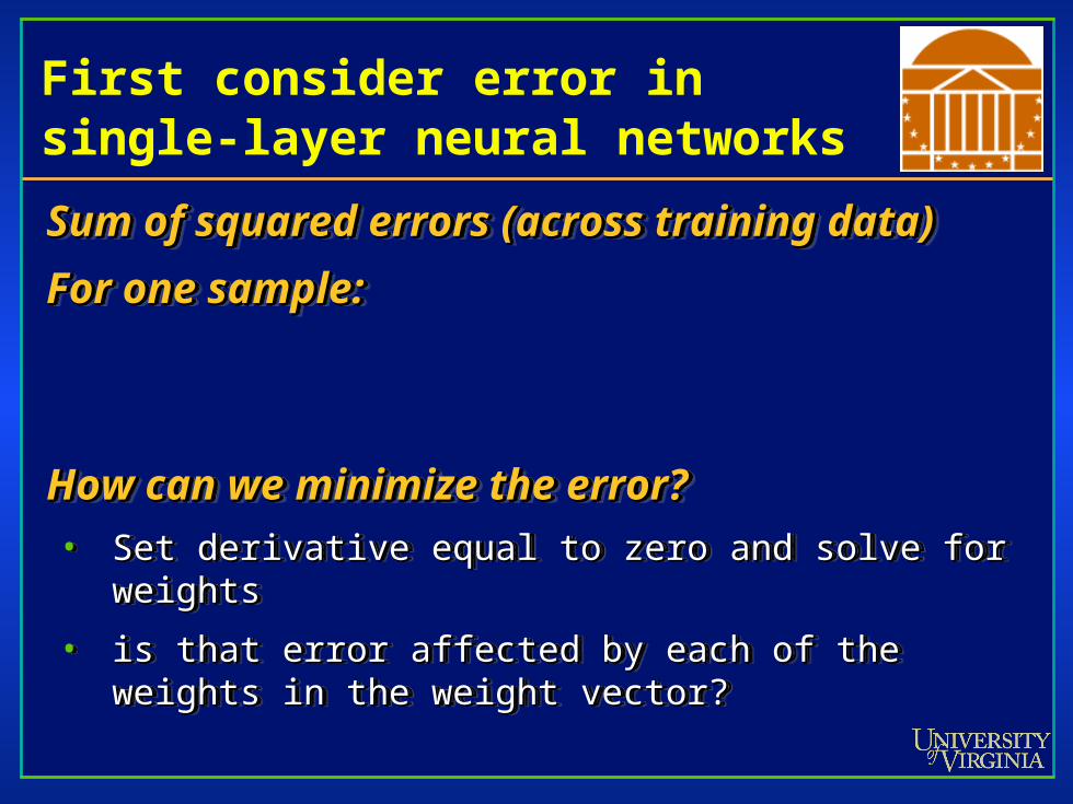
Sum of squared errors (across training data)Sum of squared errors (across training data)
For one sample:For one sample:
How can we minimize the error?How can we minimize the error?• Set derivative equal to zero and solve for weightsSet derivative equal to zero and solve for weights
• is that error affected by each of the weights in the is that error affected by each of the weights in the weight vector? weight vector?
Minimizing the error
What is the derivative?What is the derivative?
• The gradient,The gradient,
– Composed of Composed of
What is the derivative?What is the derivative?
• The gradient,The gradient,
– Composed of Composed of
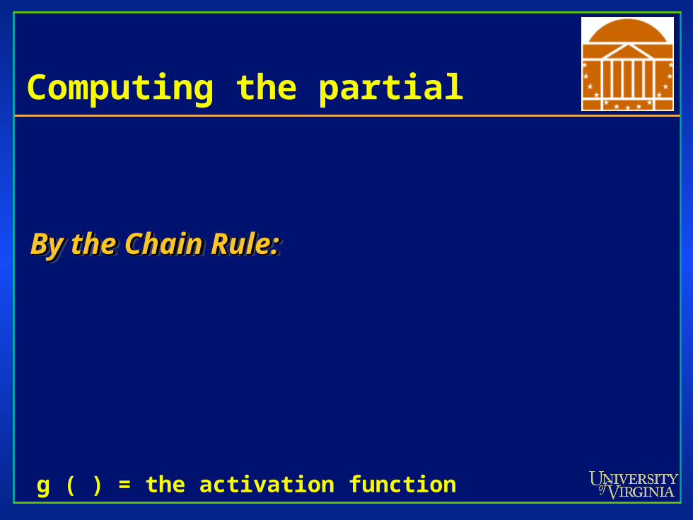
Computing the partial
By the Chain Rule: By the Chain Rule: By the Chain Rule: By the Chain Rule:
g ( ) = the activation function
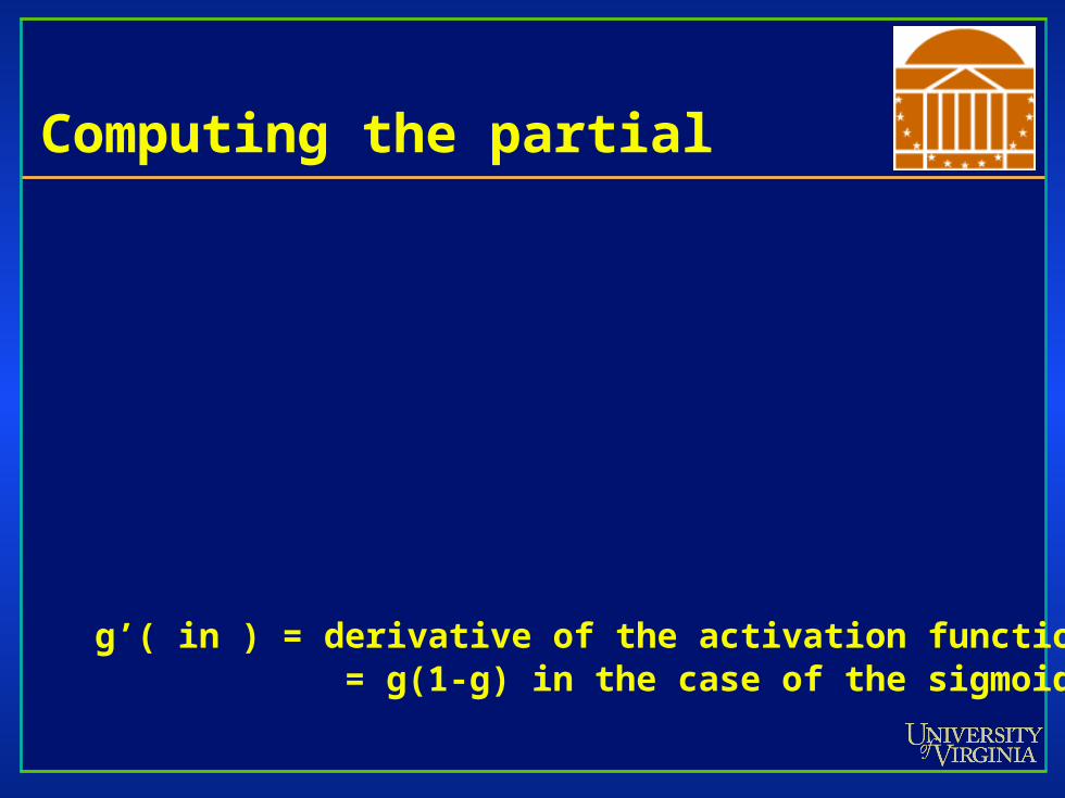
Computing the partial
g’( in ) = derivative of the activation function = g(1-g) in the case of the sigmoid
Minimizing the error
Gradient descentGradient descentGradient descentGradient descent
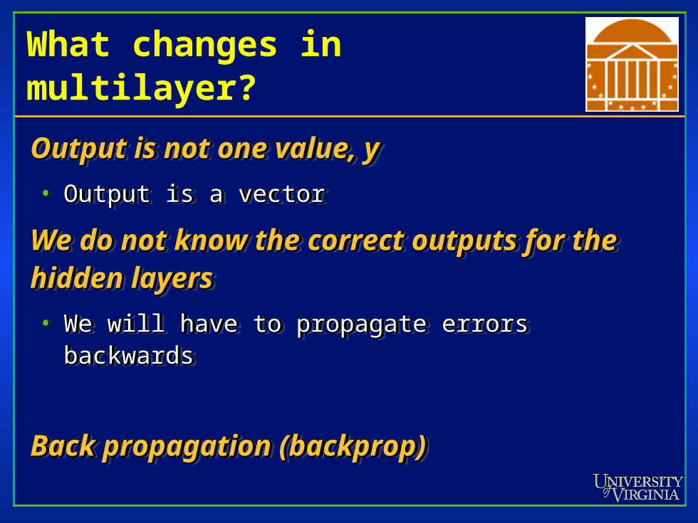
What changes in multilayer?
Output is not one value, yOutput is not one value, y
• Output is a vectorOutput is a vector
We do not know the correct outputs for the We do not know the correct outputs for the hidden layershidden layers
• We will have to propagate errors backwardsWe will have to propagate errors backwards
Back propagation (backprop)Back propagation (backprop)
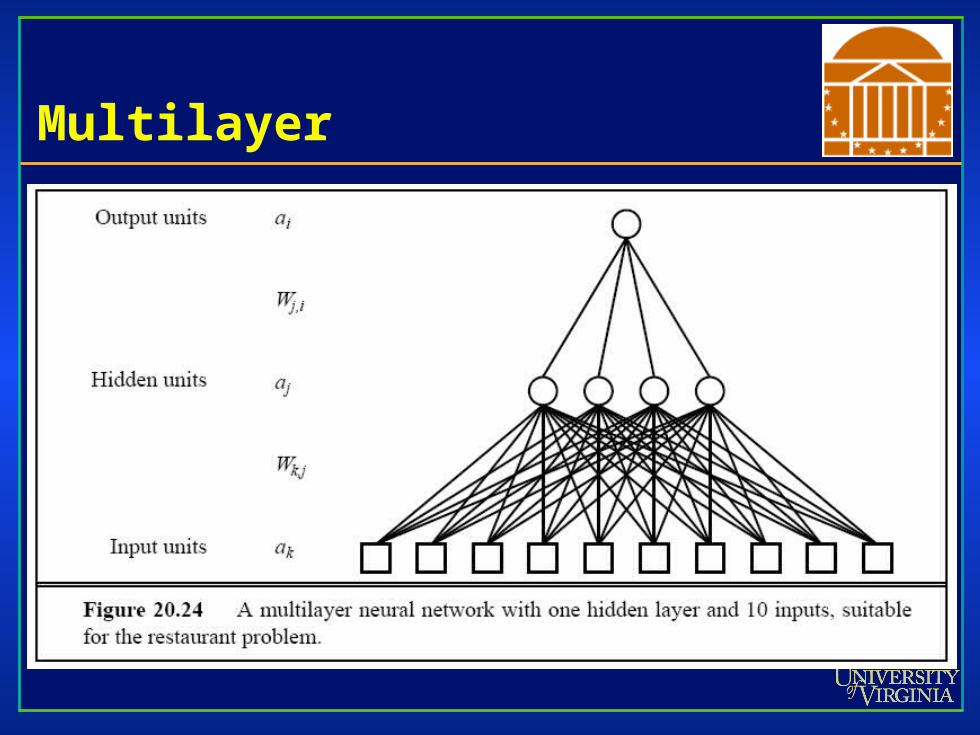
Multilayer
Backprop at the output layer
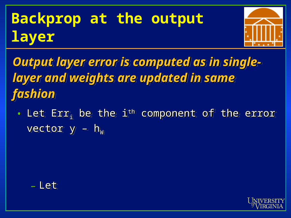
Output layer error is computed as in single-Output layer error is computed as in single-layer and weights are updated in same layer and weights are updated in same fashionfashion
• Let ErrLet Errii be the i be the ithth component of the error vector y – h component of the error vector y – hWW
– LetLet
Backprop in the hidden layer
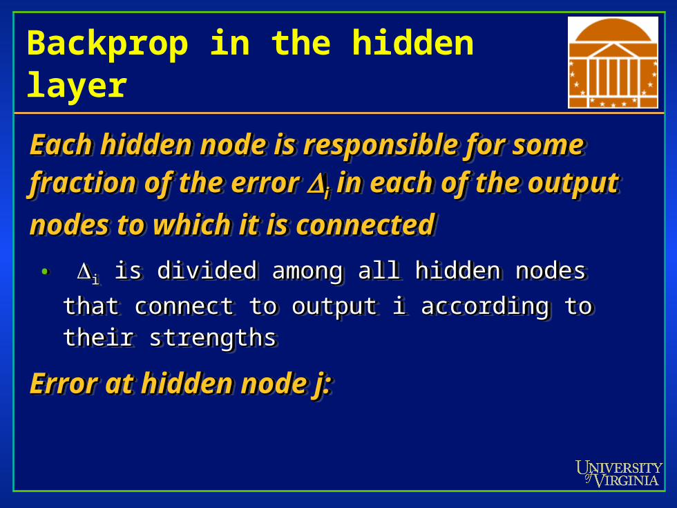
Each hidden node is responsible for some Each hidden node is responsible for some fraction of the error fraction of the error ii in each of the output in each of the output
nodes to which it is connectednodes to which it is connected
• ii is divided among all hidden nodes that connect to is divided among all hidden nodes that connect to
output i according to their strengthsoutput i according to their strengths
Error at hidden node j:Error at hidden node j:

Backprop in the hidden layer
Error is:Error is:
Correction is: Correction is:
Error is:Error is:
Correction is: Correction is:
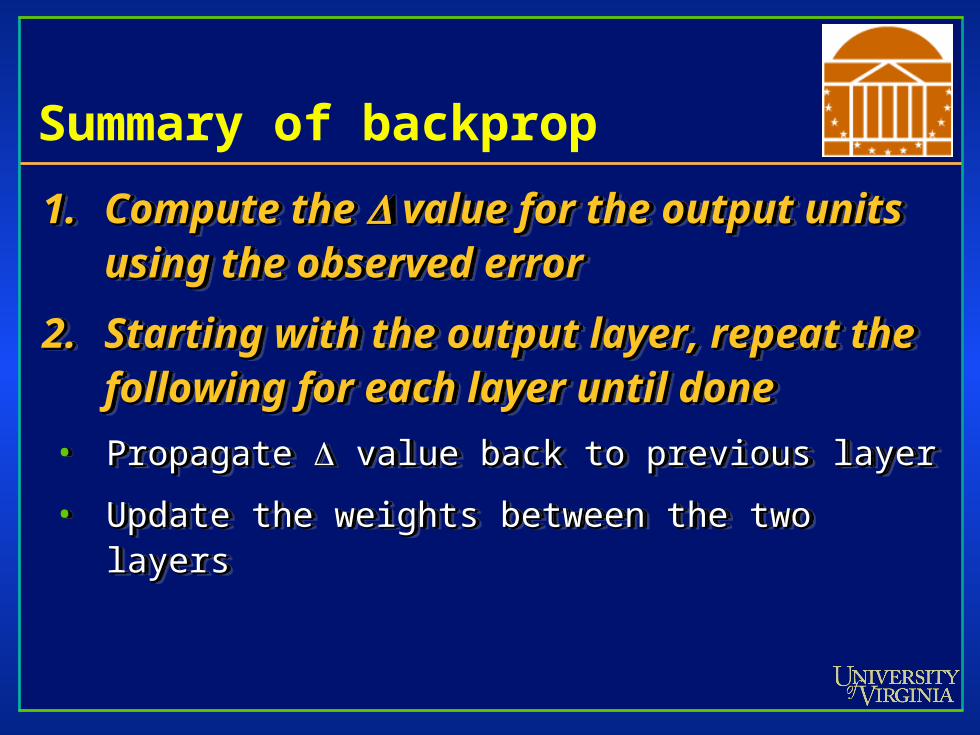
Summary of backprop
1.1. Compute the Compute the value for the output units value for the output units using the observed errorusing the observed error
2.2. Starting with the output layer, repeat the Starting with the output layer, repeat the following for each layer until donefollowing for each layer until done
• Propagate Propagate value back to previous layer value back to previous layer
• Update the weights between the two layersUpdate the weights between the two layers
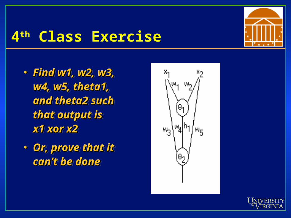
4th Class Exercise
• Find w1, w2, w3, Find w1, w2, w3, w4, w5, theta1, w4, w5, theta1, and theta2 such and theta2 such that output is that output is x1 xor x2x1 xor x2
• Or, prove that it Or, prove that it can’t be donecan’t be done
• Find w1, w2, w3, Find w1, w2, w3, w4, w5, theta1, w4, w5, theta1, and theta2 such and theta2 such that output is that output is x1 xor x2x1 xor x2
• Or, prove that it Or, prove that it can’t be donecan’t be done
Back-Propagation (xor)
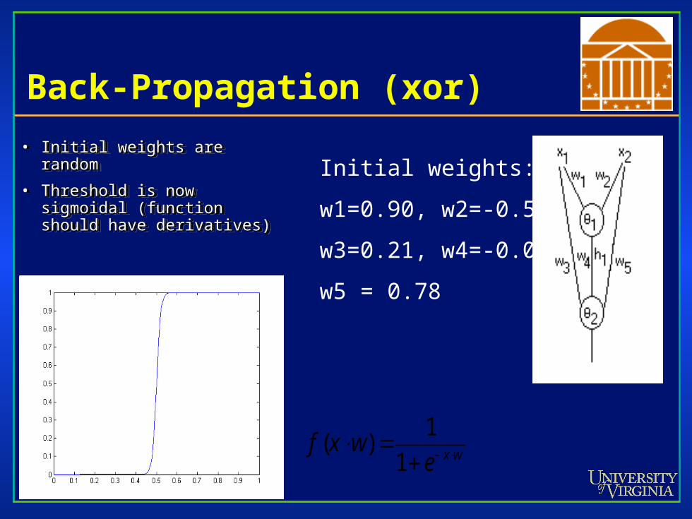
• Initial weights are randomInitial weights are random
• Threshold is now Threshold is now sigmoidal (function should sigmoidal (function should have derivatives)have derivatives)
• Initial weights are randomInitial weights are random
• Threshold is now Threshold is now sigmoidal (function should sigmoidal (function should have derivatives)have derivatives)
Initial weights:
w1=0.90, w2=-0.54
w3=0.21, w4=-0.03
w5 = 0.78
wxewxf
1
1)(
Back-Propagation (xor)
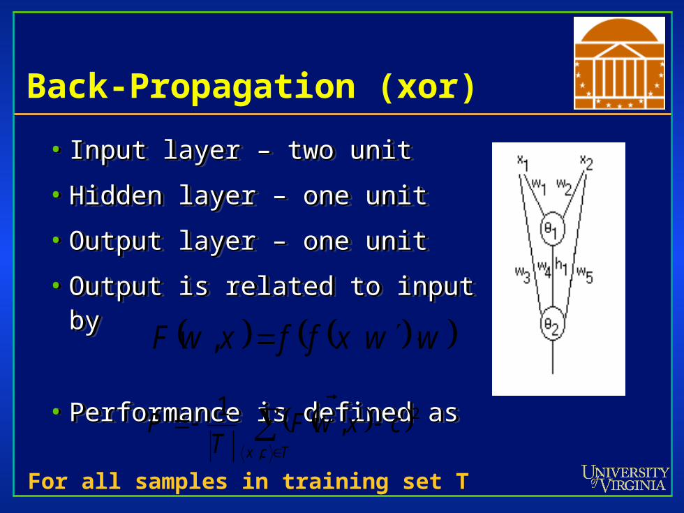
• Input layer – two unitInput layer – two unit
• Hidden layer – one unitHidden layer – one unit
• Output layer – one unitOutput layer – one unit
• Output is related to input byOutput is related to input by
• Performance is defined asPerformance is defined as
• Input layer – two unitInput layer – two unit
• Hidden layer – one unitHidden layer – one unit
• Output layer – one unitOutput layer – one unit
• Output is related to input byOutput is related to input by
• Performance is defined asPerformance is defined as
wwxffxwF ,
Tcx
cxwFT
P,
2,1
For all samples in training set T
Back-Propagation (xor)
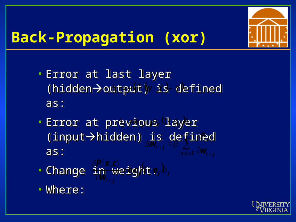
• Error at last layer (hiddenError at last layer (hiddenoutput) is output) is defined as:defined as:
• Error at previous layer (inputError at previous layer (inputhidden) hidden) is defined as:is defined as:
• Change in weight:Change in weight:
• Where:Where:
• Error at last layer (hiddenError at last layer (hiddenoutput) is output) is defined as:defined as:
• Error at previous layer (inputError at previous layer (inputhidden) hidden) is defined as:is defined as:
• Change in weight:Change in weight:
• Where:Where:
cxwF ,1
kkkkjj oow 1
Tcx ji
cx
ji w
Pw
,
,
jjjiji
ooow
cxP
1,
Back-Propagation (xor)
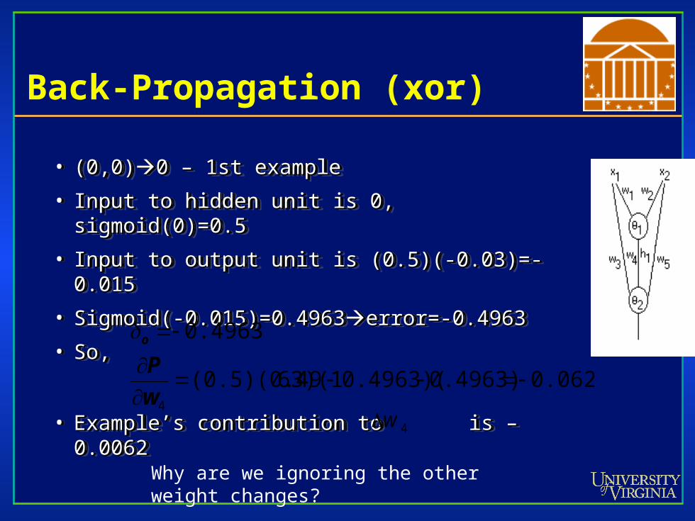
• (0,0)(0,0)0 – 1st example0 – 1st example
• Input to hidden unit is 0, sigmoid(0)=0.5Input to hidden unit is 0, sigmoid(0)=0.5
• Input to output unit is (0.5)(-0.03)=-0.015Input to output unit is (0.5)(-0.03)=-0.015
• Sigmoid(-0.015)=0.4963Sigmoid(-0.015)=0.4963error=-0.4963error=-0.4963
• So,So,
• Example’s contribution to is –0.0062Example’s contribution to is –0.0062
0.06200.4963)0.4963)(63)(1(0.5)(0.49
0.4963
4
w
Po
Why are we ignoring the other weight changes?
4w
Back-Propagation (xor)
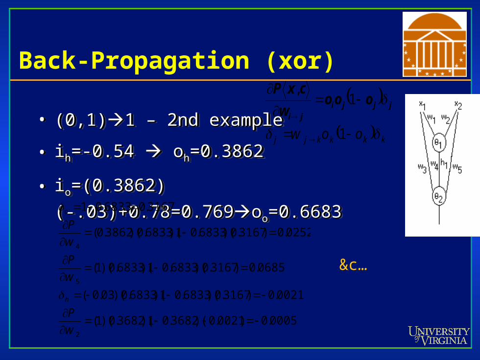
• (0,1)(0,1)1 – 2nd example1 – 2nd example
• iihh=-0.54 =-0.54 o ohh=0.3862=0.3862
• iioo=(0.3862)(-.03)+0.78=0.769=(0.3862)(-.03)+0.78=0.769oooo=0.6683=0.6683
• (0,1)(0,1)1 – 2nd example1 – 2nd example
• iihh=-0.54 =-0.54 o ohh=0.3862=0.3862
• iioo=(0.3862)(-.03)+0.78=0.769=(0.3862)(-.03)+0.78=0.769oooo=0.6683=0.6683
0005.0)0021.0)(3682.01)(3682.0)(1(
0021.0)3167.0)(6833.01)(6833.0)(03.0(
0685.0)3167.0)(6833.01)(6833.0)(1(
0252.0)3167.0)(6833.01)(6833.0)(3862.0(
3167.06833.01
2
5
4
wP
wP
wP
h
o
&c…&c…
jjjiji
ooow
cxP
1,
kkkkjj oow 1
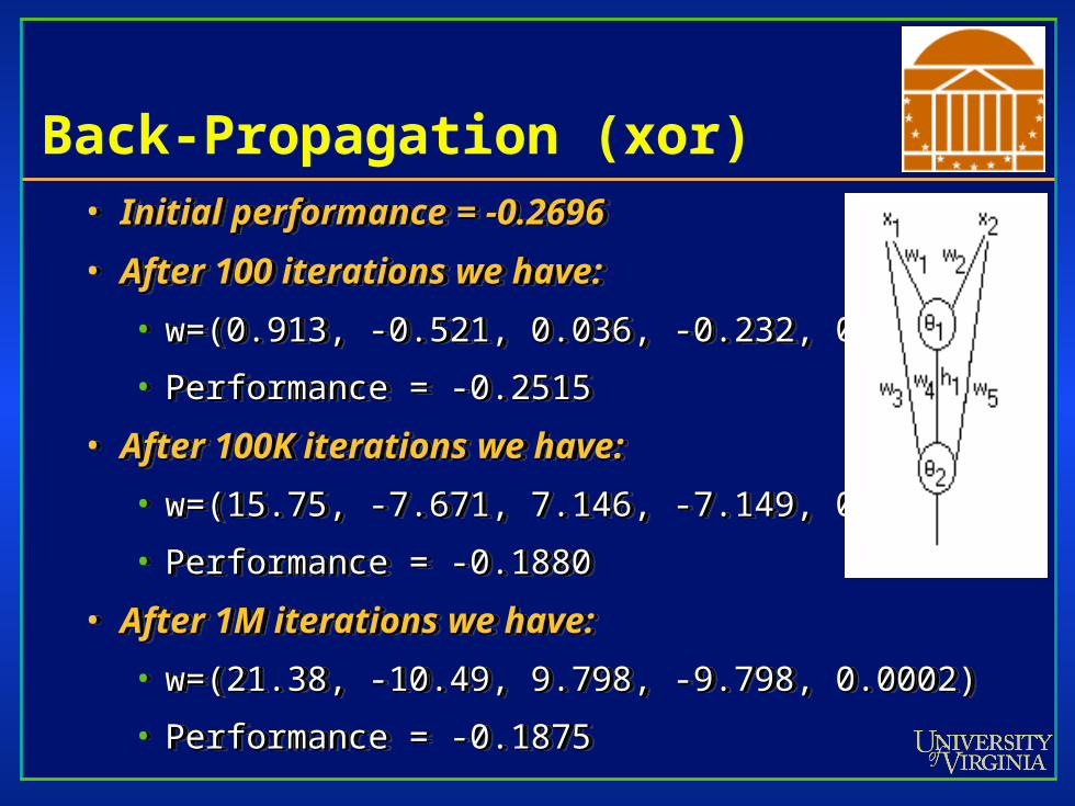
Back-Propagation (xor)• Initial performance = -0.2696Initial performance = -0.2696
• After 100 iterations we have:After 100 iterations we have:
• w=(0.913, -0.521, 0.036, -0.232, 0.288)w=(0.913, -0.521, 0.036, -0.232, 0.288)
• Performance = -0.2515Performance = -0.2515
• After 100K iterations we have:After 100K iterations we have:
• w=(15.75, -7.671, 7.146, -7.149, 0.0022)w=(15.75, -7.671, 7.146, -7.149, 0.0022)
• Performance = -0.1880Performance = -0.1880
• After 1M iterations we have:After 1M iterations we have:
• w=(21.38, -10.49, 9.798, -9.798, 0.0002)w=(21.38, -10.49, 9.798, -9.798, 0.0002)
• Performance = -0.1875Performance = -0.1875
• Initial performance = -0.2696Initial performance = -0.2696
• After 100 iterations we have:After 100 iterations we have:
• w=(0.913, -0.521, 0.036, -0.232, 0.288)w=(0.913, -0.521, 0.036, -0.232, 0.288)
• Performance = -0.2515Performance = -0.2515
• After 100K iterations we have:After 100K iterations we have:
• w=(15.75, -7.671, 7.146, -7.149, 0.0022)w=(15.75, -7.671, 7.146, -7.149, 0.0022)
• Performance = -0.1880Performance = -0.1880
• After 1M iterations we have:After 1M iterations we have:
• w=(21.38, -10.49, 9.798, -9.798, 0.0002)w=(21.38, -10.49, 9.798, -9.798, 0.0002)
• Performance = -0.1875Performance = -0.1875
Some general artificial neural network (ANN) info
• The entire network is a function g( inputs ) = outputsThe entire network is a function g( inputs ) = outputs
– These functions frequently have sigmoids in themThese functions frequently have sigmoids in them
– These functions are frequently differentiableThese functions are frequently differentiable
– These functions have coefficients (weights)These functions have coefficients (weights)
• Backpropagation networks are simply ways to tune the Backpropagation networks are simply ways to tune the coefficients of a function so it produces desired outputcoefficients of a function so it produces desired output
Function approximation
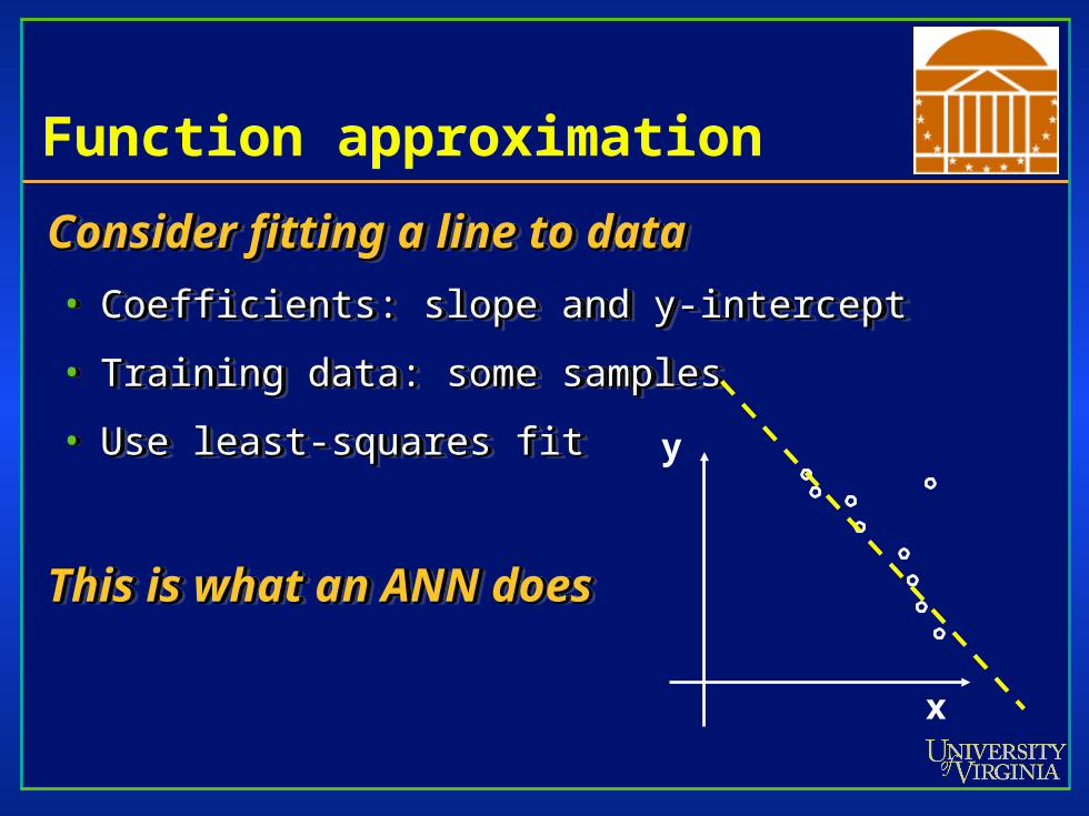
Consider fitting a line to dataConsider fitting a line to data
• Coefficients: slope and y-interceptCoefficients: slope and y-intercept
• Training data: some samplesTraining data: some samples
• Use least-squares fitUse least-squares fit
This is what an ANN doesThis is what an ANN does
Consider fitting a line to dataConsider fitting a line to data
• Coefficients: slope and y-interceptCoefficients: slope and y-intercept
• Training data: some samplesTraining data: some samples
• Use least-squares fitUse least-squares fit
This is what an ANN doesThis is what an ANN does
x
y
Function approximation
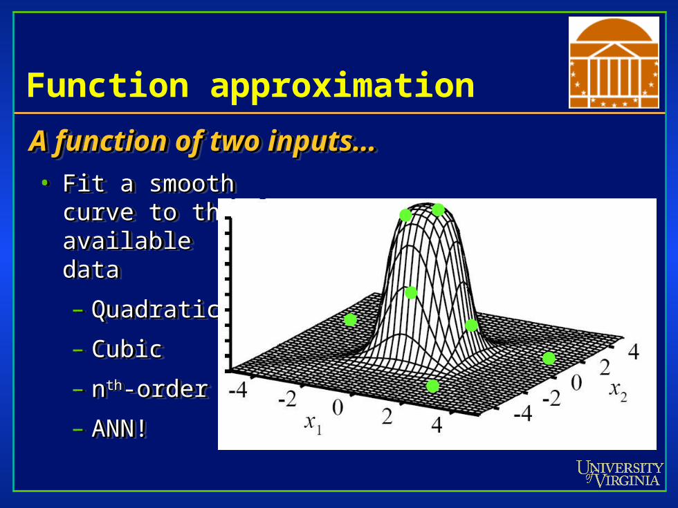
A function of two inputs…A function of two inputs…• Fit a smoothFit a smooth
curve to thecurve to theavailableavailabledatadata
– QuadraticQuadratic
– CubicCubic
– nnthth-order-order
– ANN!ANN!
A function of two inputs…A function of two inputs…• Fit a smoothFit a smooth
curve to thecurve to theavailableavailabledatadata
– QuadraticQuadratic
– CubicCubic
– nnthth-order-order
– ANN!ANN!
Curve fitting
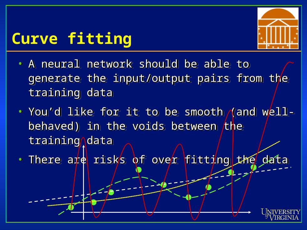
• A neural network should be able to generate the A neural network should be able to generate the input/output pairs from the training datainput/output pairs from the training data
• You’d like for it to be smooth (and well-behaved) in the You’d like for it to be smooth (and well-behaved) in the voids between the training datavoids between the training data
• There are risks of over fitting the dataThere are risks of over fitting the data
When using ANNs
• Sometimes the output layer feeds back into the input Sometimes the output layer feeds back into the input layer – recurrent neural networkslayer – recurrent neural networks
• The backpropagation will tune the weightsThe backpropagation will tune the weights
• You determine the topologyYou determine the topology
– Different topologies have different training outcomes Different topologies have different training outcomes (consider overfitting)(consider overfitting)
– Sometimes a genetic algorithm is used to explore Sometimes a genetic algorithm is used to explore the space of neural network topologiesthe space of neural network topologies
What is the Purpose of NN?
To create an Artificial Intelligence, orTo create an Artificial Intelligence, or
• Although not an invalid purpose, many people in the AI Although not an invalid purpose, many people in the AI community think neural networks do not provide anything community think neural networks do not provide anything that cannot be obtained through other techniquesthat cannot be obtained through other techniques
– It is hard to unravel the “intelligence” behind why the It is hard to unravel the “intelligence” behind why the ANN worksANN works
To study how the human brain works?To study how the human brain works?
• Ironically, those studying neural networks with this in mind Ironically, those studying neural networks with this in mind are more likely to contribute to the previous purposeare more likely to contribute to the previous purpose
Some Brain Facts
• Contains ~100,000,000,000 neuronsContains ~100,000,000,000 neurons
• Hippocampus CA3 region contains Hippocampus CA3 region contains ~3,000,000 neurons~3,000,000 neurons
• Each neuron is connected to ~10,000 other Each neuron is connected to ~10,000 other neuronsneurons
• ~ (10~ (101515)(10)(101515) connections!) connections!
• Consumes ~20-30% of the body’s energyConsumes ~20-30% of the body’s energy
• Contains about 2% of the body’s massContains about 2% of the body’s mass