CS 589Information Risk Management

30 January 2007

References for Today

• The Gaffney and Ulvila paper

• Gelman, Carlin, Stern, and Rubin, Bayesian Data Analysis. Chapman and Hall, 1998.

• Any decent statistics book that deals with Bayesian ideas

Today

• Continue with our introductory example

• Discuss the paper

• Specify Risks Using Probability Distributions

– Event Risk(s)

– Outcome Risk(s)

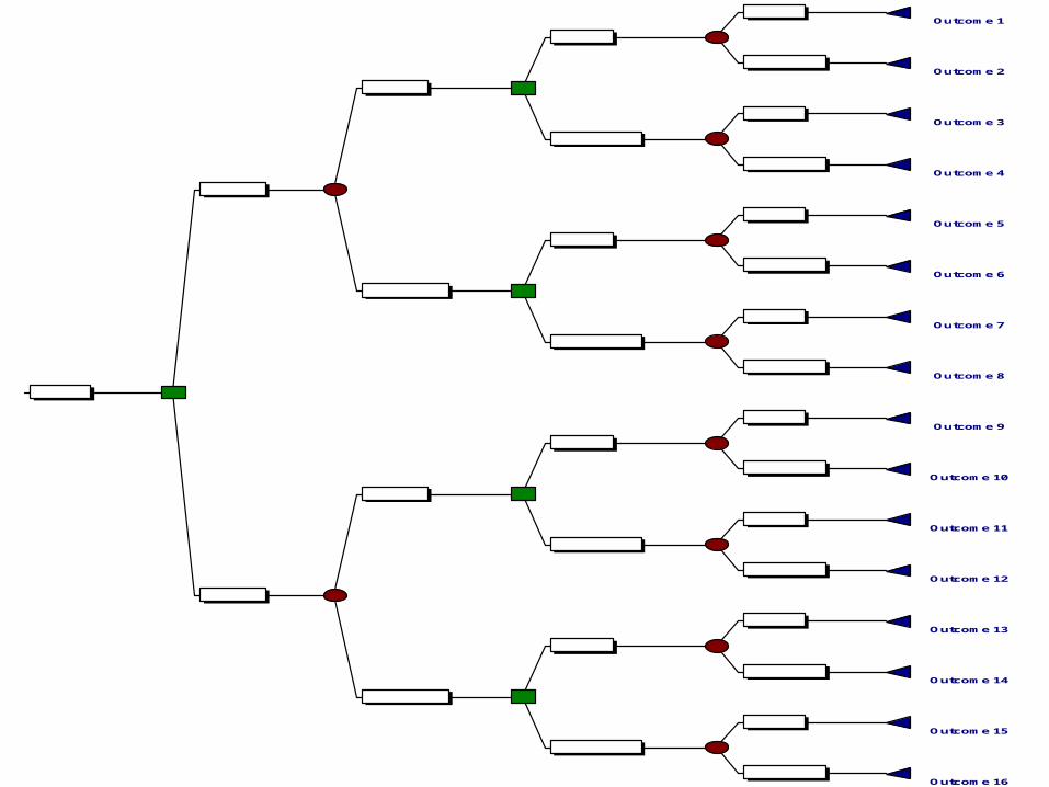
• Use our Risk Models in decision tree(s)

Outcome 1

Outcome 2

Outcome 3

Outcome 4

Outcome 5

Outcome 6

Outcome 7

Outcome 8

Outcome 9

Outcome 10

Outcome 11

Outcome 12

Outcome 13

Outcome 14

Outcome 15

Outcome 16

Example

System 1

System 2

Detection

No Detection

Respond

No Response

Respond

No Response

Intrusion

No Intrusion

Intrusion

No Intrusion

Intrusion

No Intrusion

Intrusion

No Intrusion

Detection

No Detection

Respond

No Response

Respond

No Response

Intrusion

No Intrusion

Intrusion

No Intrusion

Intrusion

No Intrusion

Intrusion

No Intrusion

What do we need to know?

• Probabilities– P(Detection|An Intrusion) P(D|I)– Associated Info– P(I)– And, finally, P(I|D)

• Outcomes– Individually, these will not be stochastic – for now– They will still lead to an expectation for each

decision node

Conditional Probability

• P(D|I) and P(D| Not I)

• P(Not D|I) and P(Not D|Not I)

• Where would we get this information?

• What about P(I)?

Bayes Rule – Simple Version

)()|(

)()|()(

)()(|

|

IPIDP

IPIDPDP

DPIPIDP

DIP

Bayes’ Rule

• Prior Idea Information Revised Idea

Information New Revision etc.

• Specific form for computing new probabilities

• Where does the prior come from? Information?

Interpretation

• Two types of Accuracy

• Two types of Error

)|()|(

)|()|(

IDPIDP

IDPIDP

Solving the Tree

• Establish the Outcomes

• Compute the Probabilities – the conditionals on the endpoints and others

• Find Expected Values and roll back the tree

Outcomes

• These will often have to be estimated

• We can follow the paper (and some convention) and incorporate costs for false positives and false negatives

• Where would we get these numbers in an actual analysis?

• What did the authors (of the paper) do?

P(I) 0.3 0.953177258 0.285

P(D|I) 0.95 0 0

P(D not|I not) 0.98 TRUE Chance

C(No Intrusion) 0 0 -0.468227425

C(Intrusion) 100 0.046822742 0.014

C(False Positive) 10 -10 -10

0.299 Decision

0 -0.468227425 0.953177258 0

-100 -100

FALSE Chance

0 -95.31772575

0.046822742 0

0 0

TRUE Chance 0 -1.64

0.021398003 0

0 0

FALSE Chance

0 -9.786019971

0.978601997 0

-10 -10

0.701 Decision 0 -2.139800285

0.021398003 0.015

-100 -100

TRUE Chance

0 -2.139800285

0.978601997 0.686

0 0

System 1

Detection

No Detection

Respond

No Response

Intrusion

No Intrusion

Respond

No Response

Intrusion

No Intrusion

Intrusion

No Intrusion

Intrusion

No Intrusion

Sensitivity Analysis

• What are the strategies given the numbers we used in the example?

• What are the key variables?

• How would we assess the base-case outcome of this example?

P(I) 0.9 0.997666278 0.855

P(D|I) 0.95 0 0

P(D not|I not) 0.98 TRUE Chance

C(No Intrusion) 0 0 -0.023337223

C(Intrusion) 100 0.002333722 0.002

C(False Positive) 10 -10 -10

0.857 Decision

0 -0.023337223 0.997666278 0

-100 -100

FALSE Chance

0 -99.76662777

0.002333722 0

0 0

TRUE Chance 0 -1

0.314685315 0.045

0 0

TRUE Chance

0 -6.853146853

0.685314685 0.098

-10 -10

0.143 Decision 0 -6.853146853

0.314685315 0

-100 -100

FALSE Chance

0 -31.46853147

0.685314685 0

0 0

System 1

Detection

No Detection

Respond

No Response

Intrusion

No Intrusion

Respond

No Response

Intrusion

No Intrusion

Intrusion

No Intrusion

Intrusion

No Intrusion

P(I) 0.9 0.997666278 0.855

P(D|I) 0.95 0 0

P(D not|I not) 0.98 TRUE Chance

C(No Intrusion) 0 0 -0.023337223

C(Intrusion) 1000 0.002333722 0.002

C(False Positive) 10 -10 -10

0.857 Decision

0 -0.023337223 0.997666278 0

-1000 -1000

FALSE Chance

0 -997.6662777

0.002333722 0

0 0

TRUE Chance 0 -1

0.314685315 0.045

0 0

TRUE Chance

0 -6.853146853

0.685314685 0.098

-10 -10

0.143 Decision 0 -6.853146853

0.314685315 0

-1000 -1000

FALSE Chance

0 -314.6853147

0.685314685 0

0 0

System 1

Detection

No Detection

Respond

No Response

Intrusion

No Intrusion

Respond

No Response

Intrusion

No Intrusion

Intrusion

No Intrusion

Intrusion

No Intrusion

P(I) 0 0 0

P(D|I) 0.95 0 0

P(D not|I not) 0.98 FALSE Chance

C(No Intrusion) 0 0 -10

C(Intrusion) 1000 1 0

C(False Positive) 10 -10 -10

0.02 Decision

0 0 0 0

-1000 -1000

TRUE Chance

0 0

1 0.02

0 0

TRUE Chance 0 0

0 0

0 0

FALSE Chance

0 -10

1 0

-10 -10

0.98 Decision 0 0

0 0

-1000 -1000

TRUE Chance

0 0

1 0.98

0 0

System 1

Detection

No Detection

Respond

No Response

Intrusion

No Intrusion

Respond

No Response

Intrusion

No Intrusion

Intrusion

No Intrusion

Intrusion

No Intrusion

Don’t Forget the Bottom Line

• Our decision criterion – Expected Cost

• We want to see what happens under different circumstances

• We can even show these situations – scenarios – graphically

• Relationships between cost ratio and P(D|I) and P(D not|I not)

Expected Costs Given Detector Accuracy and Cost Ratio

-9

-8

-7

-6

-5

-4

-3

-2

-1

0

0 0.1 0.2 0.3 0.4 0.5 0.6 0.7 0.8 0.9 1

P(Intrusion)

E(C

ost)

.95,.98,100

.95,.98,1000

.98,.95,100

.98,.95,1000

Different Conditional Information

• What if we don’t know P(D|I)?

• We can flip the tree according to what we do know

• Outcomes should remain the same

• And the decision should remain the same

Another Way – Info Dependent

)()|(

)()|()(

)(|

|

IPIDP

IPIDPDP

DPIPDIP

IDP

Modeling

• Decisions, chance events

• Probability distributions for chance events– Lack of data Bayesian methods– Expert(s)– Lots of data Distribution model(s)

• Outcomes– Financial, if possible– Multiple measures/criteria/attributes

Decision Situation

• In the context of Firm or Organization Goals, Objectives, Strategies

• A complete understanding should lead to a 1-2 sentence Problem Definition– Could be risk-centered– Could be oriented toward larger info issues

• Problem Definition should drive the selection of Alternatives and, to some degree, how they are evaluated

Information Business Issues

• Integrity and reliability of information stored and used in systems

• Preserve privacy and confidentiality

• Enhance availability of other information systems

Risk Management

• Process of defining and measuring or assessing risk and developing strategies to mitigate or minimize the risk

• Defining and assessing– Data driven– Other sources

• Developing strategies– Done in context of objectives, goals

What About the Paper?

• What is the problem/model structure?

• What are the key risks?

• How were they modeled?

• What do the authors say about the structure of the problem?

• What conclusions do you draw from the paper?

Probability Models

• For events

– Discrete Events

– Poisson Distribution

– Binomial Distribution

• For outcomes

• Combine with Bayesian analysis

Poisson Distribution

!)(

ke

kXPk

Poisson Distribution

• Independent events happen along a continuum– Time – often the case in IA– Space– Distance

• Distribution parameter is the expected number of events per unit

• Parameter is also the distribution variance

• One possible model for discrete data

Poisson Distributions

0

0.05

0.1

0.15

0.2

0.25

0.3

0.35

0.4

0 1 2 3 4 5 6 7 8k

P(X

=k|la

mbd

a)

lambda =1lambda =2lambda =3lambda =4

Using the Poisson in IRM

• Probability model of events per unit of measurement

• Expected number of events might impact technology choice

• Range of potential events might impact tech choice

• If we are risk averse, distributions help us explicitly consider event risks

Events in a 24-Hour Period

0

1

2

3

4

5

6

7

1 3 5 7 9 11 13 15 17 19 21 23

Hour

Eve

nts

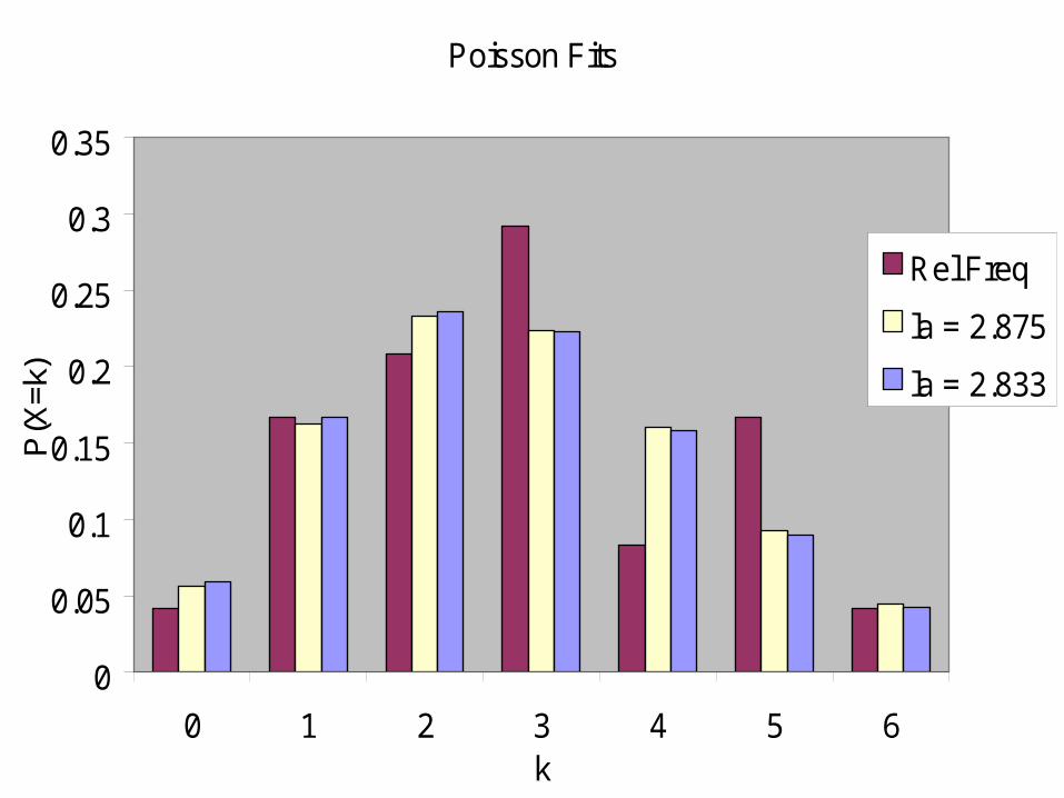
Poisson Fits

0

0.05

0.1

0.15

0.2

0.25

0.3

0.35

0 1 2 3 4 5 6k

P(X

=k)

Rel Freq

la = 2.875

la = 2.833

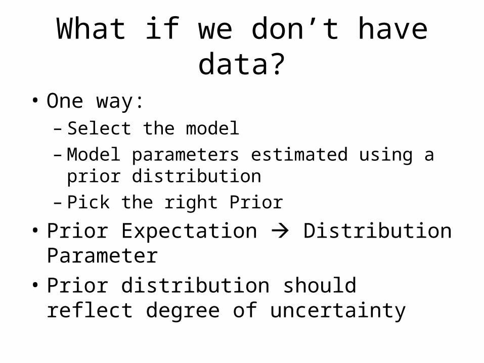
What if we don’t have data?

• One way:– Select the model– Model parameters estimated using a prior

distribution– Pick the right Prior

• Prior Expectation Distribution Parameter

• Prior distribution should reflect degree of uncertainty

Priors

• Prior for a Poisson parameter is Gamma

0,)(

)(

0)(

1)(

0

1

/1

xE

dxex

xexxf

x

x

Gamma(16, .125)

0.0

0.1

0.2

0.3

0.4

0.5

0.6

0.7

0.8

0.9

0.0

0.5

1.0

1.5

2.0

2.5

3.0

3.5

4.0

4.5

5.0

>5.0% 5.0%90.0%1.254 2.887

Gamma(2, 1)

0.00

0.05

0.10

0.15

0.20

0.25

0.30

0.35

0.40

0 1 2 3 4 5 6 7 8

>5.0%90.0%0.355 4.744

Gamma(64, .03125)

0.0

0.2

0.4

0.6

0.8

1.0

1.2

1.4

1.6

1.8

0 1 2 3 4 5 6 7 8

>5.0% 5.0%90.0%1.607 2.428

Prior Distribution

• The prior should reflect our degree of certainty, or degree of belief, about the parameter we are estimating

• One way to deal with this is to consider distribution fractiles

• Use fractiles to help us develop the distribution that reflects the synthesis of what we know and what we believe

Prior + Information

• As we collect information, we can update our prior distribution and get a – we hope – more informative posterior distribution

• Recall what the distribution is for – in this case, a view of our parameter of interest

• The posterior mean is now the estimate for the Poisson lambda, and can be used in decision-making

Information

• For our Poisson parameter, information might consist of data similar to what we already collected in our example

• We update the Gamma, take the mean, and that’s our new estimate for the average occurrences of the event per unit of measurement.

Next Time

• You guys will present your responses to the homework assignment

• We will continue with Bayesian analysis and another example or two

• Segue into other topics given our framework that we have developed