CS D6: Topics in Risk Identification and Risk Measurement for Insurers

***Property/Casualty Underwriting Risk

John KollarERM Symposium

May 3, 2005

Underlying Themes• Underwriting is the primary source of risk

for a P/C insurer.• Risk = uncertainty in results• The insurer’s risk is measured by the

stochastic distribution of possible outcomes.

• Amount of risk amount of capital.• Capital is an expense as it must be paid

for.• Develop strategy to make the most efficient

use of capital = maximize return vs. risk.

Components of Underwriting Risk• Loss volatility including

– Catastrophe and non-catastrophe risk – Risk of adverse loss development for long-

tailed lines• How long the capital has to be held to

support reserve risk• Correlation between lines (dependencies)• Pricing risk (underwriting cycle)

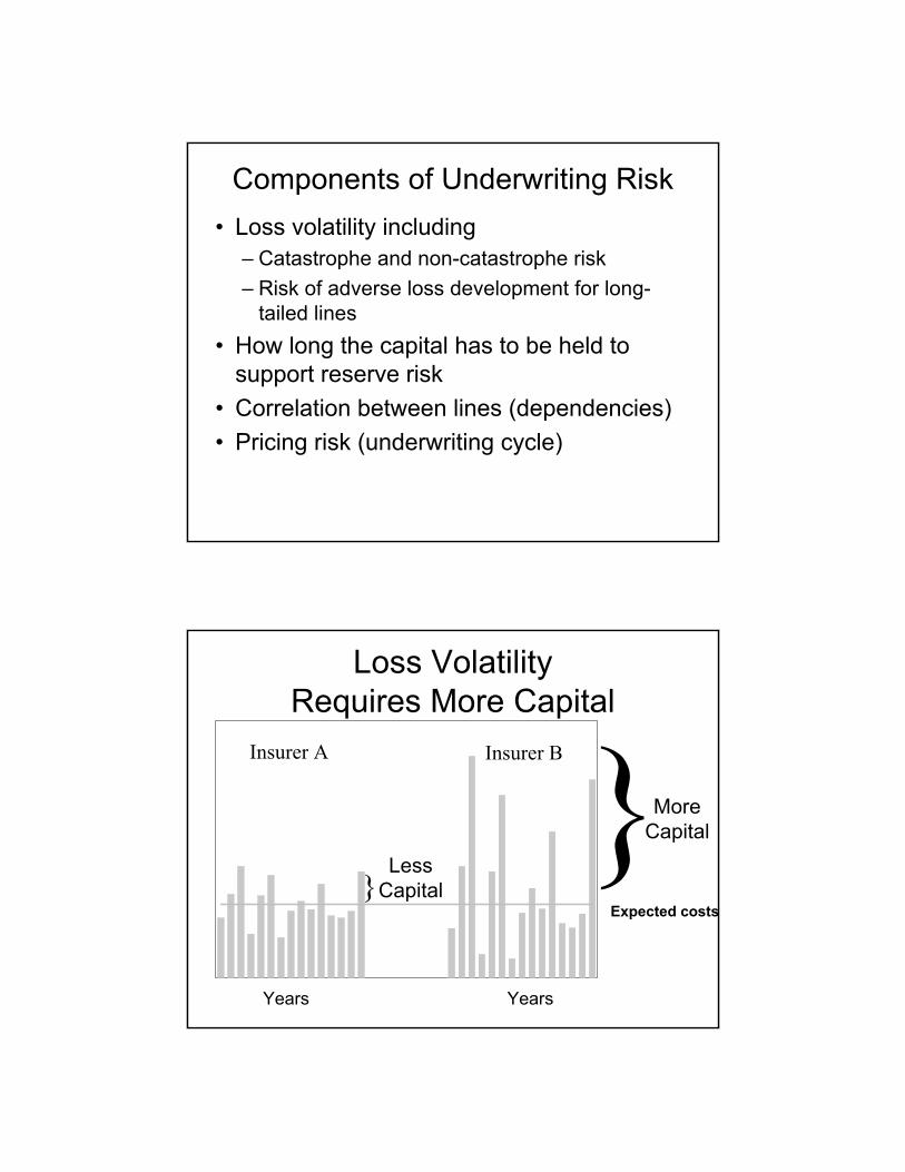
Loss Volatility Requires More Capital

}}Less

Capital

More Capital

Expected costs

Insurer A Insurer B

Years Years

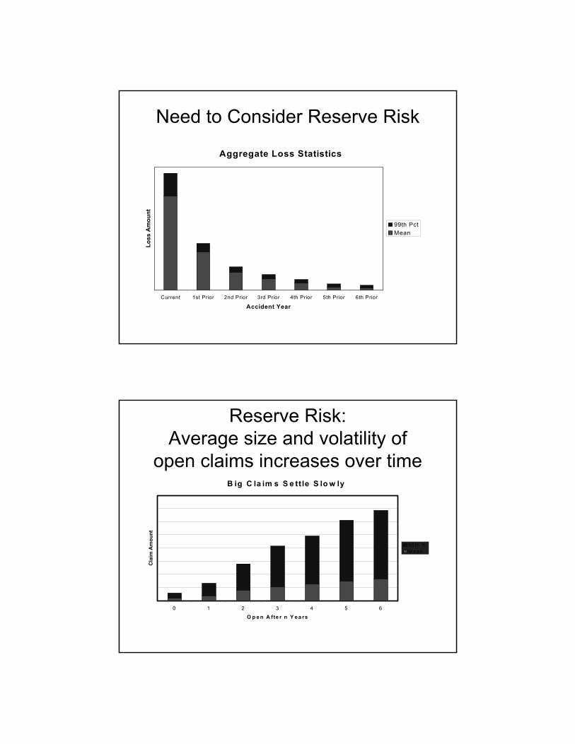
Need to Consider Reserve Risk

Aggregate Loss Statistics

Current 1st Prior 2nd Prior 3rd Prior 4th Prior 5th Prior 6th Prior

Accident Year

Loss

Am

ount

99th PctMean

Reserve Risk:Average size and volatility of

open claims increases over timeB ig C la im s S e ttle S lo w ly

0 1 2 3 4 5 6

O p e n A fte r n Y e a rs

Cla

im A

mou

nt

9 5 th %M e a n

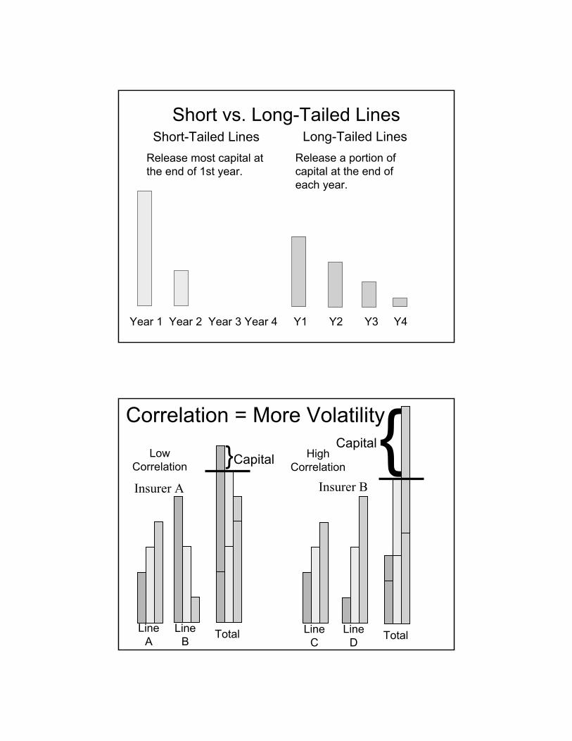
Short vs. Long-Tailed LinesShort-Tailed Lines

Release most capital at the end of 1st year.

Long-Tailed LinesRelease a portion of capital at the end of each year.

Year 1 Year 2 Year 3 Year 4 Y1 Y2 Y3 Y4

Correlation = More Volatility

LineA

LineB

LineC

LineD Total

{Capital}CapitalLow Correlation

HighCorrelation

Total

Insurer A Insurer B

Correlation• Law of Large Numbers: increased

volume (larger insurers)– Lower process risk– Higher correlation

• Greater concentration of exposures = increased catastrophe risk for property insurance, WC, group life

• Diversification– Reduced correlation/concentration– Higher expenses

Correlation increases with volume

C orre la tion and R isk S ize

0.00

0 .02

0 .04

0 .06

0 .08

0 .10

0 .12

0 .14

0 .16

0 .18

0 .20

S ize o f R isk

Cor

rela

tion

Measuring Underwriting Risk• Use industry data to develop claim

severity distributions:– By line (product)– By valuation (settlement lag)

• Use data by company (for many companies) to develop claim frequency parameters:– By line– By valuation– Measure correlations by size of insurer

using common shock models to develop covariance generators between lines.

Measuring an Insurer’s Underwriting Risk

• For each line of insurance: – Select a random claim count.– Select random claim size for each claim.– Adjust claim size for coverage limits and

reinsurance.• The aggregate loss for all lines = sum of all the

random claim amounts for all lines.– Reflect the correlation between lines (products).

• Use a Catastrophe Model to generate many years of catastrophe losses.

Measuring an Insurer’s Underwriting Risk (Cont’d)

• Generate an aggregate loss distribution.• Or simulate many years of aggregate

losses.• Or simulate many years of individual

losses.

Measuring an Insurer’s Underwriting Risk (Cont’d)

• What is the tolerance for risk?– Regulatory requirement (RBC)– “A” rating from a rating agency– Tradition, etc.

• Select a statistical measure of risk that corresponds to the tolerance for risk.– Value at risk (VAR)– Tail value at risk (TVAR)– Standard deviation, etc.

• Determine total capital for underwriting from the aggregate loss distribution using the selected measure of risk.

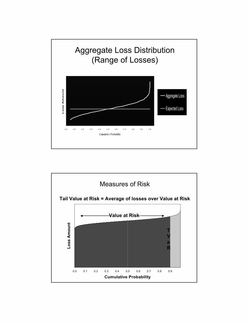
Aggregate Loss Distribution (Range of Losses)

0 . 0 0 0 . 1 0 0 . 2 0 0 . 3 0 0 . 4 0 0 . 5 0 0 . 6 0 0 . 7 0 0 . 8 0 0 . 9 0 1 . 0 0

C um ula t iv e P ro ba bility

Lo

ss A

mo

un

t

Aggregate Loss

Expected Loss

0.0 0.1 0.2 0.3 0.4 0.5 0.6 0.7 0.8 0.9

Cumulative Probability

Loss

Am

ount

Measures of Risk

Tail Value at Risk = Average of losses over Value at Risk

Value at Risk

TVaR

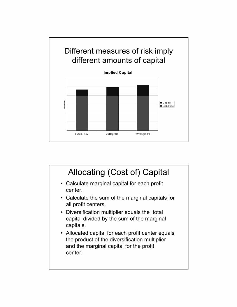
Different measures of risk imply different amounts of capital

Implied Capital

2xStd. Dev. VaR@99% TVaR@99%

Am

ount Capital

Liabilities

Allocating (Cost of) Capital• Calculate marginal capital for each profit

center.• Calculate the sum of the marginal capitals for

all profit centers.• Diversification multiplier equals the total

capital divided by the sum of the marginal capitals.

• Allocated capital for each profit center equals the product of the diversification multiplier and the marginal capital for the profit center.

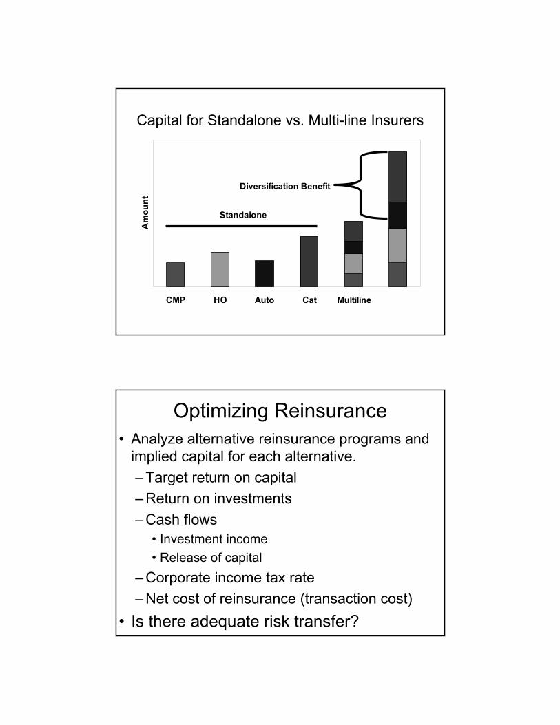
Capital for Standalone vs. Multi-line Insurers

CMP HO Auto Cat Multiline

Am

ount

Diversification Benefit

Standalone

Optimizing Reinsurance• Analyze alternative reinsurance programs and

implied capital for each alternative.– Target return on capital– Return on investments– Cash flows

• Investment income• Release of capital

– Corporate income tax rate– Net cost of reinsurance (transaction cost)

• Is there adequate risk transfer?

Consider the Time Dimension• How long must insurer hold capital?

– The longer capital is held to support a line of insurance, the greater the cost of writing the line of insurance.

– Capital can be released over time as risk is reduced.

• Investment income generated by the insurance operation– Investment income on loss reserves– Investment income on capital

Cost of Financing Risk =Cost of Capital + Net Cost of Reinsurance

• Cost of capital = target return x capital– Comparable basis to reinsurance– Discounted

• Net cost of reinsurance = Premium – Expected Recovery

• Minimize the cost of financing risk.

Optimize reinsurance by minimizing the cost of financing

Cost of Financing Insurance

No Re Cat Re All Re

Am

ount Net Cost of Reins

Cost of Capital

Setting Combined Ratio Targets by Line (Product)

• Expected losses• Expected expenses• Investment income• Cost of financing risk

– Cost of capital– Net cost of reinsurance

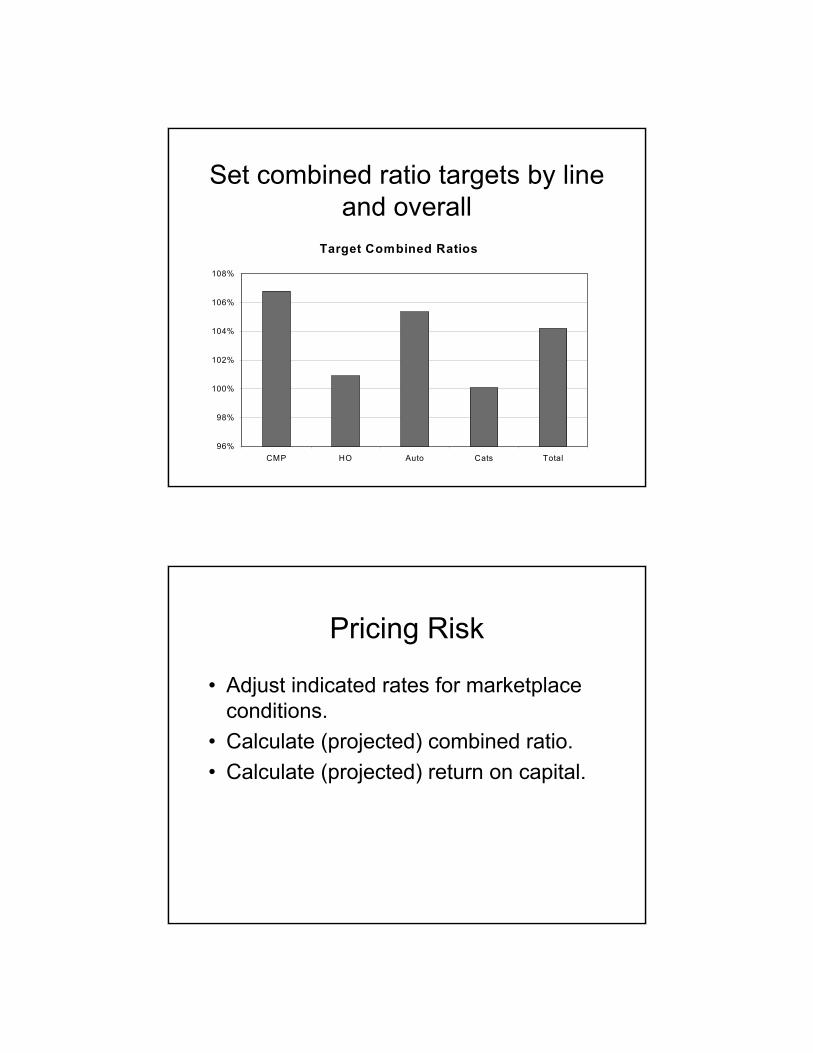
Set combined ratio targets by line and overall

Target Combined Ratios

96%

98%

100%

102%

104%

106%

108%

CMP HO Auto Cats Total

Pricing Risk

• Adjust indicated rates for marketplace conditions.

• Calculate (projected) combined ratio.• Calculate (projected) return on capital.

Planning Underwriting Strategy

• Add policies/portfolios that increase the return on capital.

• Drop policies that diminish return on capital.

• Optimize underwriting portfolio.

Reflect risk in planning growthGrowing the Business

Standalone Standalone Standalone Total Total

Req

uire

d C

apita

l

Prospect 1Prospect 2Existing

Robust Analysis of Underwriting Risk

• Board of Directors– Benchmarking

• Rating Agencies– Financial strength ratings

• Regulators– Capital requirements

• Stock Analysts– Stock recommendations

Commonalities & Differences

Property Casualty (P/C)Life

Health

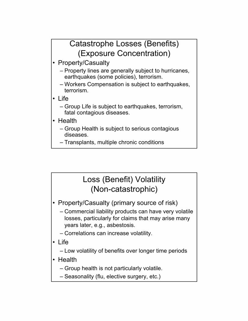
Catastrophe Losses (Benefits)(Exposure Concentration)

• Property/Casualty– Property lines are generally subject to hurricanes,

earthquakes (some policies), terrorism.– Workers Compensation is subject to earthquakes,

terrorism.• Life

– Group Life is subject to earthquakes, terrorism, fatal contagious diseases.

• Health– Group Health is subject to serious contagious

diseases.– Transplants, multiple chronic conditions

Loss (Benefit) Volatility(Non-catastrophic)

• Property/Casualty (primary source of risk)– Commercial liability products can have very volatile

losses, particularly for claims that may arise many years later, e.g., asbestosis.

– Correlations can increase volatility.• Life

– Low volatility of benefits over longer time periods• Health

– Group health is not particularly volatile.– Seasonality (flu, elective surgery, etc.)

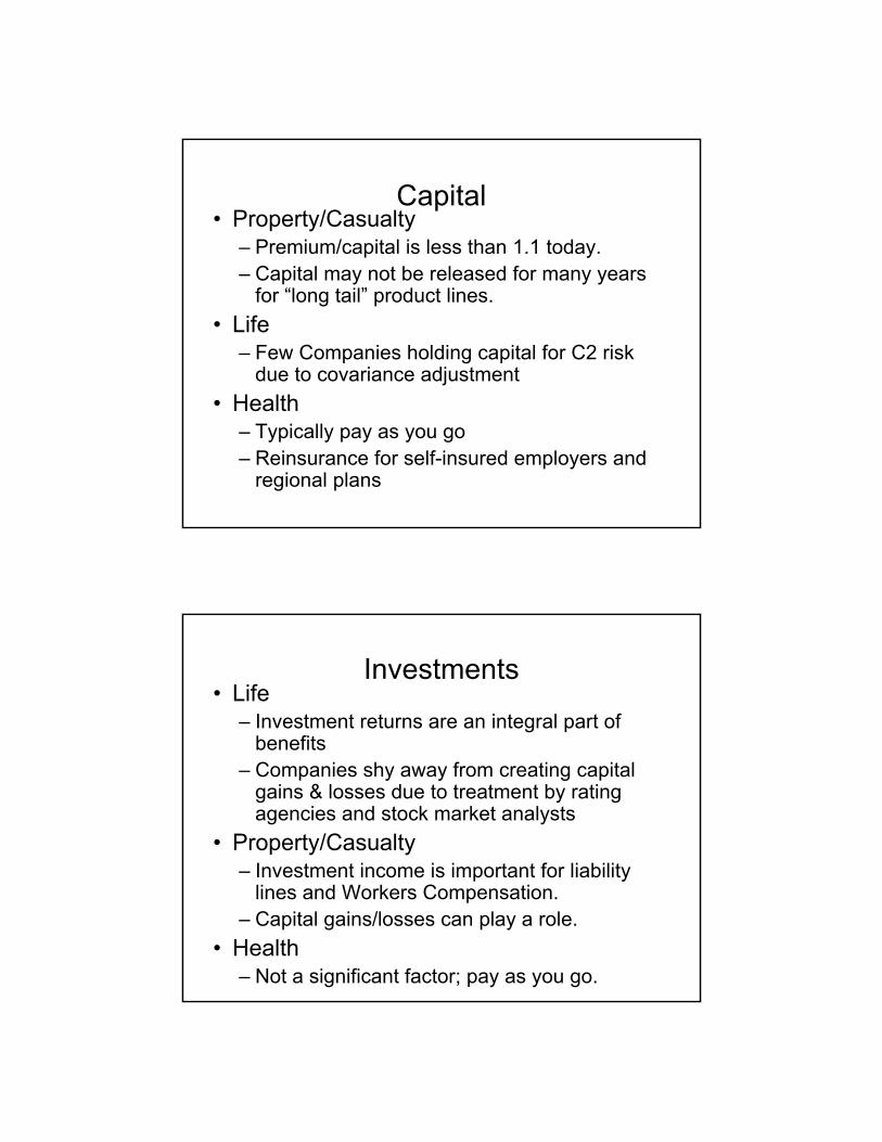
Capital• Property/Casualty

– Premium/capital is less than 1.1 today.– Capital may not be released for many years

for “long tail” product lines.• Life

– Few Companies holding capital for C2 risk due to covariance adjustment

• Health– Typically pay as you go– Reinsurance for self-insured employers and

regional plans

Investments• Life

– Investment returns are an integral part of benefits

– Companies shy away from creating capital gains & losses due to treatment by rating agencies and stock market analysts

• Property/Casualty– Investment income is important for liability

lines and Workers Compensation.– Capital gains/losses can play a role.

• Health– Not a significant factor; pay as you go.

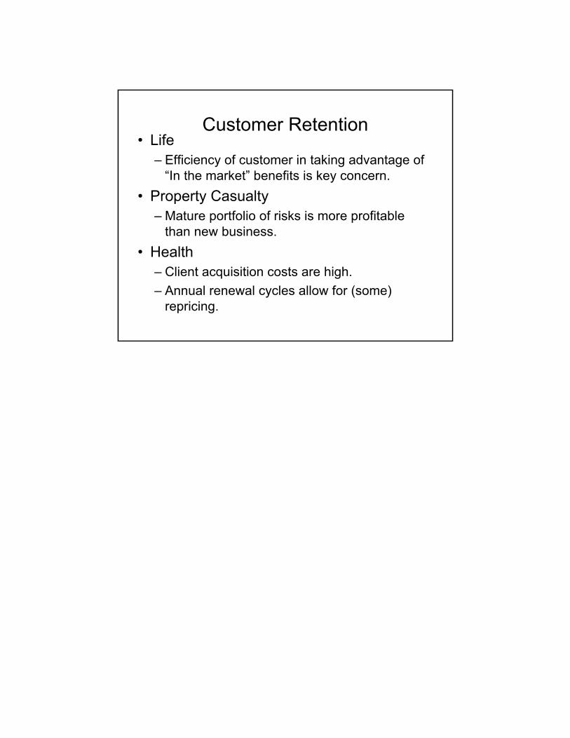
Customer Retention• Life

– Efficiency of customer in taking advantage of “In the market” benefits is key concern.

• Property Casualty– Mature portfolio of risks is more profitable

than new business.• Health

– Client acquisition costs are high.– Annual renewal cycles allow for (some)

repricing.

Mortality Risk Measurement

David Ingram, FSA, FRM, PRM

Agenda

1. Characteristics of Mortality Risk2. RBC for Mortality3. Factors that Influence Mortality Risk4. Small Group Risk5. Concentrated Group Risk6. Counterparty Risk

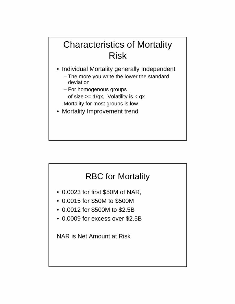
Characteristics of Mortality Risk

• Individual Mortality generally Independent– The more you write the lower the standard

deviation– For homogenous groups

of size >= 1/qx, Volatility is < qxMortality for most groups is low

• Mortality Improvement trend

RBC for Mortality

• 0.0023 for first $50M of NAR,• 0.0015 for $50M to $500M• 0.0012 for $500M to $2.5B • 0.0009 for excess over $2.5B

NAR is Net Amount at Risk

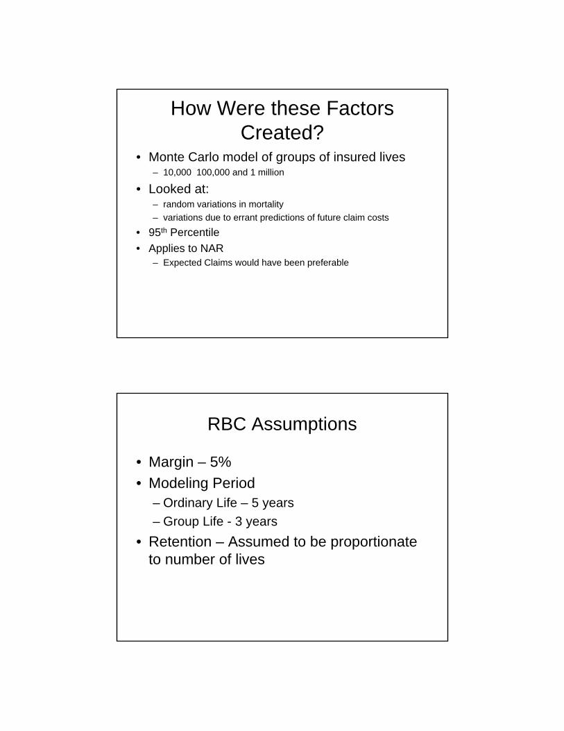
How Were these Factors Created?

• Monte Carlo model of groups of insured lives– 10,000 100,000 and 1 million

• Looked at: – random variations in mortality– variations due to errant predictions of future claim costs

• 95th Percentile• Applies to NAR

– Expected Claims would have been preferable

RBC Assumptions

• Margin – 5%• Modeling Period

– Ordinary Life – 5 years– Group Life - 3 years

• Retention – Assumed to be proportionate to number of lives

RBC Scenario Tests

• AIDS Scenarios – Variations in company AIDS exposures

• Catastrophic • Anti-Selection Lapse Spiral• Misestimation of Trend

– Competitive Risk

How accurate is RBC?

• Inaccurate for companies:– Higher or lower Average Size– Higher or lower expected claims as pct NAR– Different Spread of policy sizes– Different Retention Limit per policy– Different confidence interval on expected

claims

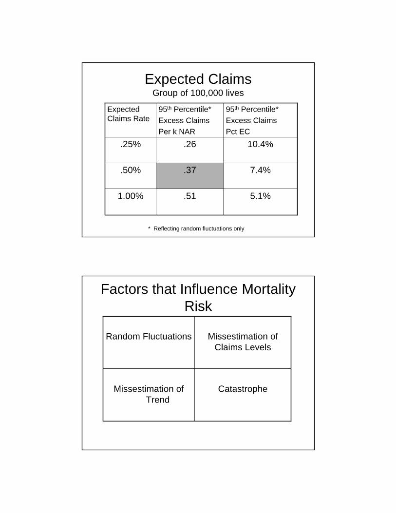
Expected ClaimsGroup of 100,000 lives

5.1%.511.00%

7.4%.37.50%

10.4%.26.25%

95th Percentile*Excess ClaimsPct EC

95th Percentile*Excess ClaimsPer k NAR

Expected Claims Rate

* Reflecting random fluctuations only

Factors that Influence Mortality Risk

CatastropheMissestimation of Trend

Missestimation of Claims Levels

Random Fluctuations

Missestimation of Mean

• Underwriting Class Assignment• Distribution within classes• Error Rate Measurement

• Experience and Testing• Use of Chi squared Test• Higher confidence in expected mortality with more

measurement periods

Missestimation of Trend

Mortality Improvement Trends in USCohort Effect in UK

US Mortality Improvement

US Male Deaths per 100,000 Age Adjusted

0

500

1000

1500

2000

2500

3000

1900

1904

1908

1912

1916

1920

1924

1928

1932

1936

1940

1944

1948

1952

1956

1960

1964

1968

1972

1976

1980

1984

1988

1992

1996

2000

US Mortality Improvement

Annual Improvement in Age Adjusted Male US Death Rate

-4.00%

-3.00%

-2.00%

-1.00%

0.00%

1.00%

2.00%

3.00%

4.00%

5.00%

6.00%

1950

1953

1956

1959

1962

1965

1968

1971

1974

1977

1980

1983

1986

1989

1992

1995

1998

2001

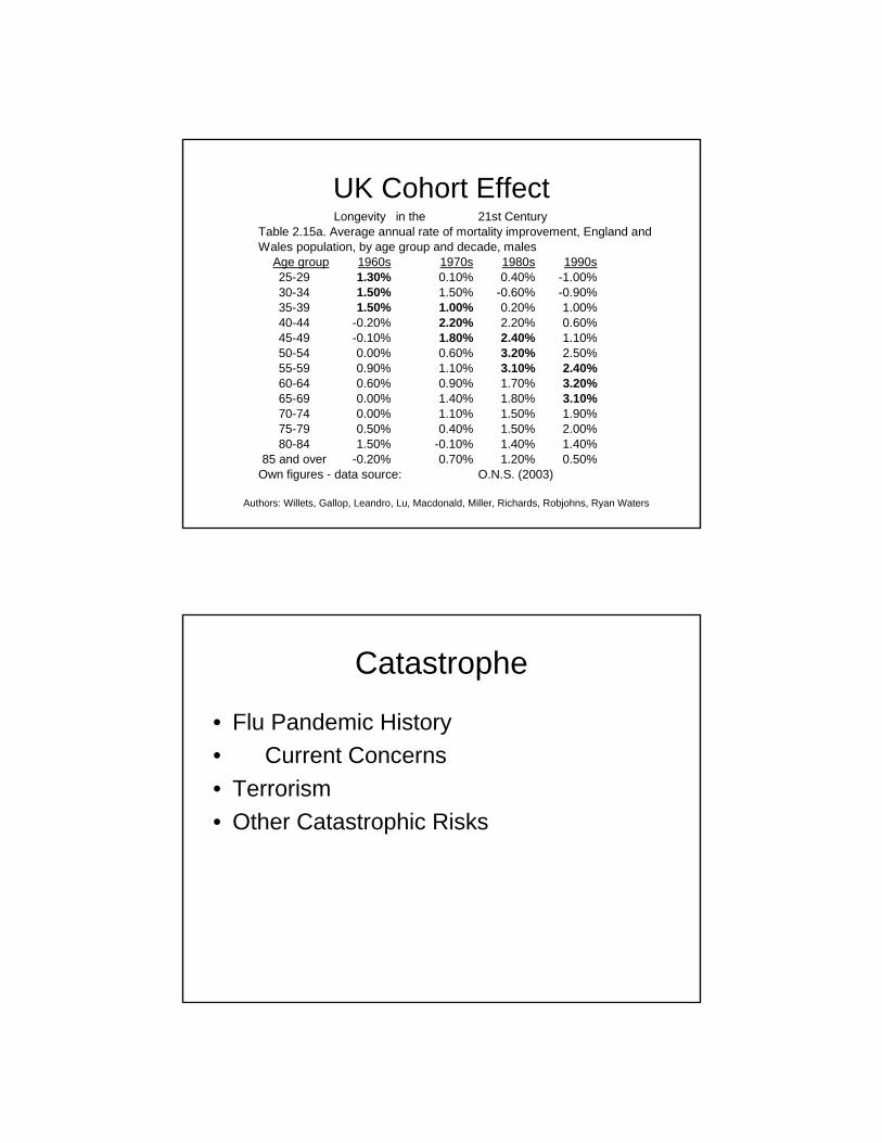
UK Cohort EffectLongevity in the 21st Century

Table 2.15a. Average annual rate of mortality improvement, England andWales population, by age group and decade, males

Age group 1960s 1970s 1980s 1990s25-29 1.30% 0.10% 0.40% -1.00%30-34 1.50% 1.50% -0.60% -0.90%35-39 1.50% 1.00% 0.20% 1.00%40-44 -0.20% 2.20% 2.20% 0.60%45-49 -0.10% 1.80% 2.40% 1.10%50-54 0.00% 0.60% 3.20% 2.50%55-59 0.90% 1.10% 3.10% 2.40%60-64 0.60% 0.90% 1.70% 3.20%65-69 0.00% 1.40% 1.80% 3.10%70-74 0.00% 1.10% 1.50% 1.90%75-79 0.50% 0.40% 1.50% 2.00%80-84 1.50% -0.10% 1.40% 1.40%

85 and over -0.20% 0.70% 1.20% 0.50%Own figures - data source: O.N.S. (2003)

Authors: Willets, Gallop, Leandro, Lu, Macdonald, Miller, Richards, Robjohns, Ryan Waters

Catastrophe

• Flu Pandemic History • Current Concerns• Terrorism• Other Catastrophic Risks

Random Fluctuations

• Impact of Size of Block of Lives• Impact of Variety of Block of lives

Mortality Risk Transfer Securities• Swiss Re Cat Bonds• Securitizations of XXX reserves• BNP Paribas Longevity Bond

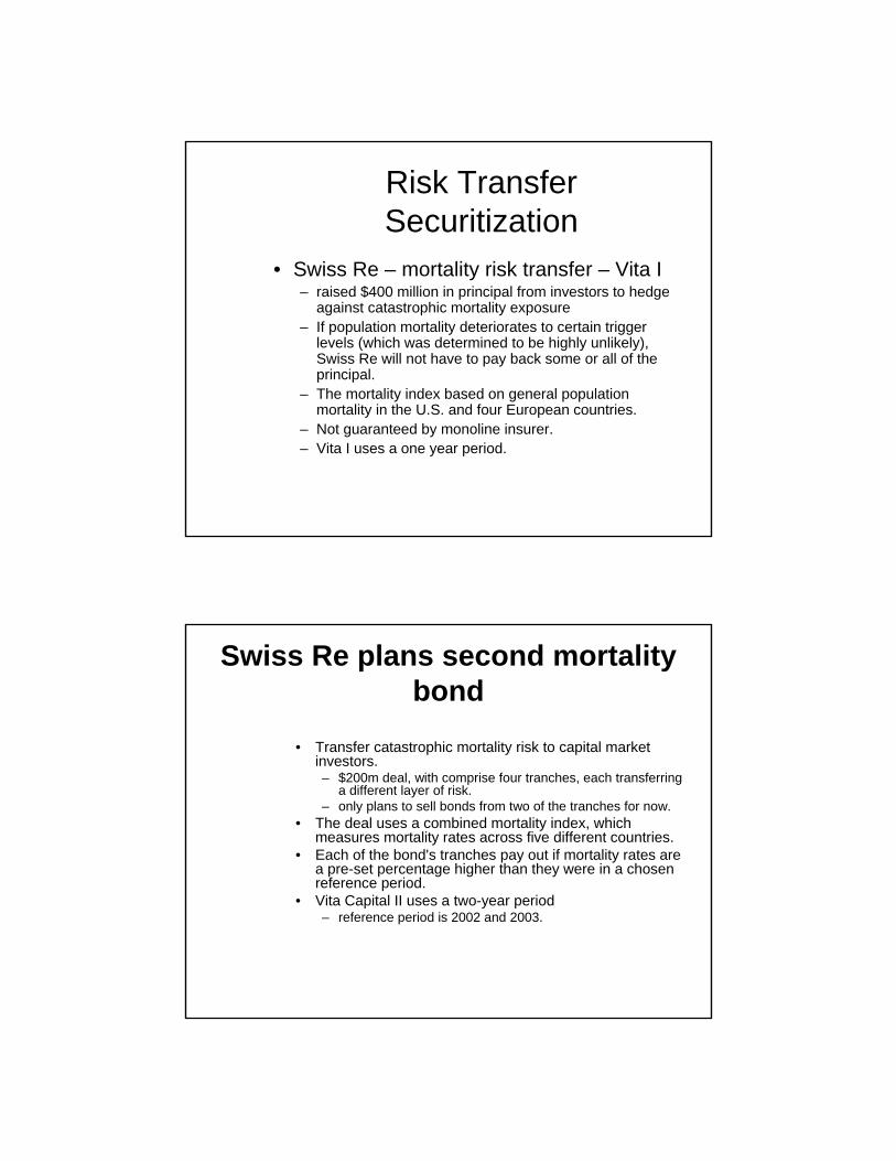
Risk Transfer Securitization

• Swiss Re – mortality risk transfer – Vita I– raised $400 million in principal from investors to hedge

against catastrophic mortality exposure – If population mortality deteriorates to certain trigger

levels (which was determined to be highly unlikely), Swiss Re will not have to pay back some or all of the principal.

– The mortality index based on general population mortality in the U.S. and four European countries.

– Not guaranteed by monoline insurer.– Vita I uses a one year period.

Swiss Re plans second mortality bond

• Transfer catastrophic mortality risk to capital market investors. – $200m deal, with comprise four tranches, each transferring

a different layer of risk. – only plans to sell bonds from two of the tranches for now.

• The deal uses a combined mortality index, which measures mortality rates across five different countries.

• Each of the bond's tranches pay out if mortality rates are a pre-set percentage higher than they were in a chosen reference period.

• Vita Capital II uses a two-year period– reference period is 2002 and 2003.

Vita Capital II• The bond's tranches are triggered if mortality rates exceed the average during this

period by certain percentages. • For example, the bond's class A notes, rated A+ by Standard & Poor's (S&P), pay out

when mortality rates during a two- year period are 125% of the average during 2002 and 2003. The notes pay out on a sliding scale until mortality rates reach 145%

• The class B notes, rated A-, are triggered when mortality rates hit 120% and they pay out up to 125%. The class C notes, rated BBB+, pay out between 115% and 120%. And the class D notes, rated BBB-, pay out between 110% and 115%.

• It would take a very serious pandemic or man-made disaster to trigger the tranches. S&P estimates that 1,077,000 more people would have to die during a two-year period than in 2002 and 2003 to trigger the class A notes. Some 860,000 more people would have to die to trigger the class B notes. It would take 646,000 more deaths to trigger the class C notes, and 430,000 more to trigger the class D notes.

Standard & Poor’s Comments

• Events such as the peak of Aids deaths in 1995, September 11 or the recent tsunami catastrophe in south-east Asia would not have triggered the bond.

• Even the 1918 influenza pandemic, which caused a 33% increase in mortality rates over a single calendar year, would not have triggered the bond.

• The rating agency believes the biggest risks are another pandemic, a full-scale ground war or several nuclear explosions. Only these types of events are likely to cause a loss for bondholders.

Vita II Structure• Swiss Re is only selling notes from class C and D for now. It will issue $100m of

bonds from each. The notes will mature in January 2010. – Swiss Re Capital Markets is the deal's lead manager and arranger. – Consultant Milliman calculated the deal's mortality risks.

• The index underpinning Vita Capital II comprises five countries.– weighted to reflect Swiss Re's exposure to these markets. – US (62.5%), the UK (17.5%), Germany (7.5%), Japan (7.5%) and Canada (5%). – also weighted to reflect the sex and age of the policyholders in Swiss Re's portfolio. A wide

range of age groups is included in the index. • The deal's structure is the same as most catastrophe bonds.

– Investors' money is held in a trust and invested in very secure short-term investments. – If the bond is triggered, the proceeds go to Swiss Re. – If it is not, the proceeds go back to investors. – The interest is paid from a combination of the return the trust makes on its safe investments

and the premium Swiss Re pays for the coverage.

Risk Transfer Securitization

• BNP Paribas – Longevity Bond– Hedges Mortality Trend Risk in UK– Partnership with EIB, BNP Paribas and

Partner Re– Bond Payoff based on ONS reported

longevity for UK 65 year old Male Cohort

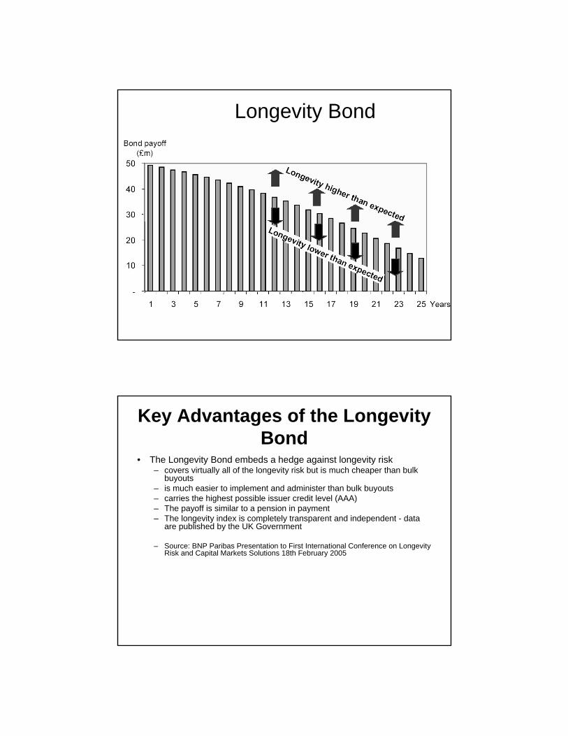
Longevity Bond

Key Advantages of the Longevity Bond

• The Longevity Bond embeds a hedge against longevity risk– covers virtually all of the longevity risk but is much cheaper than bulk

buyouts– is much easier to implement and administer than bulk buyouts– carries the highest possible issuer credit level (AAA)– The payoff is similar to a pension in payment– The longevity index is completely transparent and independent - data

are published by the UK Government

– Source: BNP Paribas Presentation to First International Conference on Longevity Risk and Capital Markets Solutions 18th February 2005

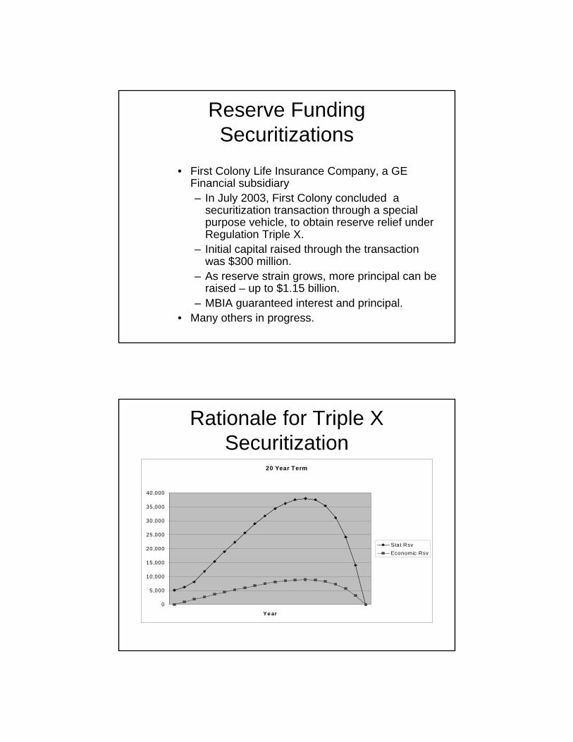
Reserve Funding Securitizations

• First Colony Life Insurance Company, a GE Financial subsidiary– In July 2003, First Colony concluded a

securitization transaction through a special purpose vehicle, to obtain reserve relief under Regulation Triple X.

– Initial capital raised through the transaction was $300 million.

– As reserve strain grows, more principal can be raised – up to $1.15 billion.

– MBIA guaranteed interest and principal.• Many others in progress.

Rationale for Triple X Securitization

20 Year Term

0

5,000

10,000

15,000

20,000

25,000

30,000

35,000

40,000

Y e ar

Stat RsvEconomic Rsv

Basics

• Assets backing redundant Triple X reserves are funded by the capital markets

• Surplus Notes issuance / redemption linked to build up / runoff of redundant reserves

• Assets backing redundant reserves invested in similar instruments used to purchase Notes

Basics

• Notes are wrapped by a monoline, with monoline agreeing to back future issuance of Notes up to specific limit as hump grows

• Includes in force business and limited amount of new business

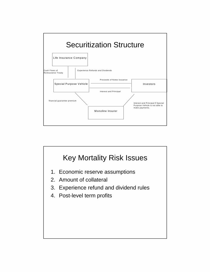
Securitization Structure

Cash Flows of Experience Refunds and D ividendsReinsurance Treaty

Proceeds of Notes Issuance

Interest and Principal

financia l guarantee prem iumInterest and Principal if SpecialPurpose Vehicle is not able to m ake paym ents.

Special Purpose Vehicle Investors

Life Insurance Com pany

M onoline Insurer

Key Mortality Risk Issues

1. Economic reserve assumptions 2. Amount of collateral3. Experience refund and dividend rules4. Post-level term profits

``

Marilyn Schlein KramerERM Symposium 2005

May 3, 2995

Promoting Fair and Efficient Health Care

Predictive Modeling in Group Health and Workers Compensation

Outline

• Compare and contrast healthcare modeling with P&C modeling

• Overview of health care model actuarial applications in group health

• Applications to Workers Comp

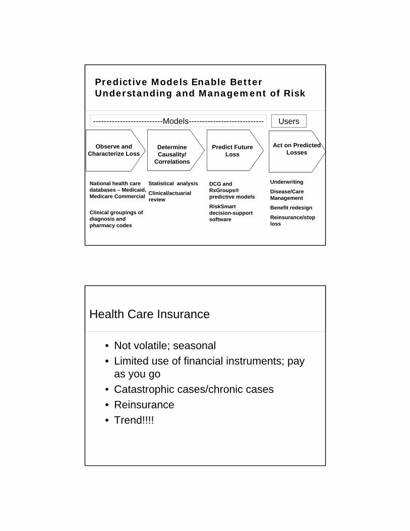
Observe and Characterize Loss

Determine Causality/

Correlations

Predict Future Loss

Act on Predicted Losses

Underwriting

Disease/Care Management

Benefit redesign

Reinsurance/stop loss

DCG and RxGroups® predictive models

RiskSmart decision-supportsoftware

Statistical analysis

Clinical/actuarialreview

National health care databases – Medicaid, Medicare Commercial

Clinical groupings of diagnosis and pharmacy codes

--------------------------Models---------------------------- Users

Predictive Models Enable Better Understanding and Management of Risk

Health Care Insurance

• Not volatile; seasonal• Limited use of financial instruments; pay

as you go • Catastrophic cases/chronic cases• Reinsurance• Trend!!!!

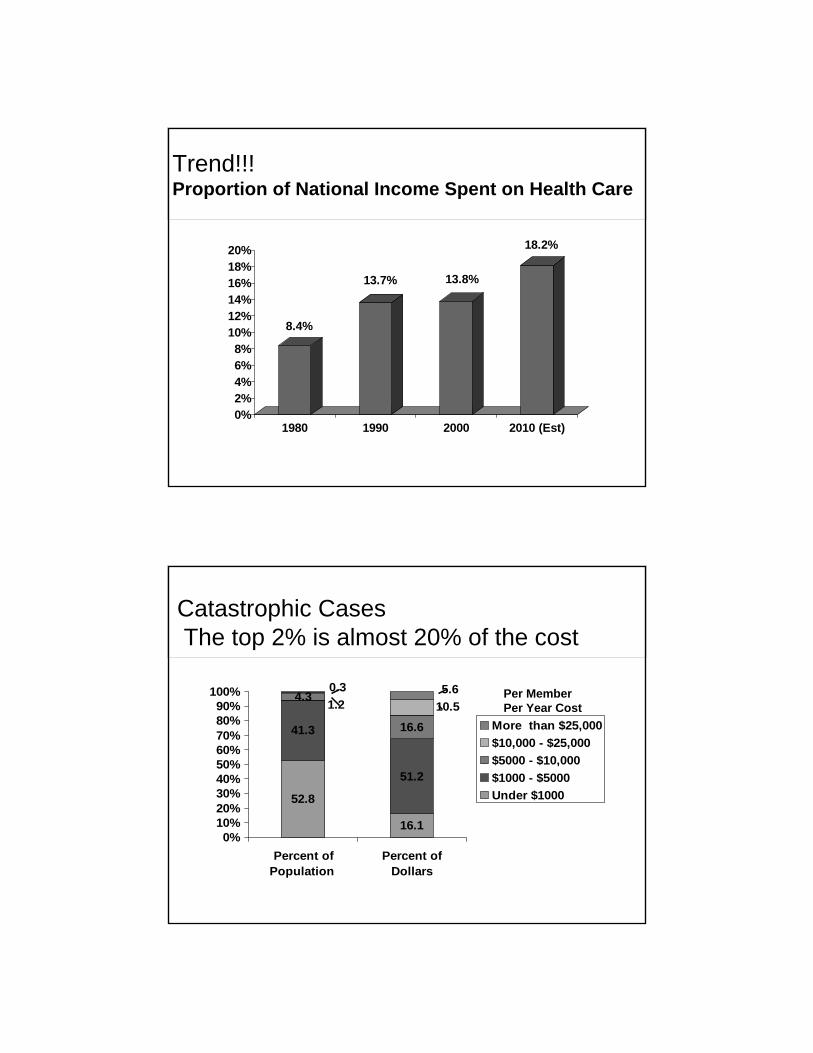
Trend!!!Proportion of National Income Spent on Health Care

8.4%

13.7% 13.8%

18.2%

0%2%4%6%8%

10%12%14%16%18%20%

1980 1990 2000 2010 (Est)

Catastrophic CasesThe top 2% is almost 20% of the cost

16.1

41.3

51.2

4.3

16.6

52.8

10.51.25.60.3

0%10%20%30%40%50%60%70%80%90%

100%

Percent ofPopulation

Percent ofDollars

More than $25,000$10,000 - $25,000$5000 - $10,000$1000 - $5000Under $1000

Per MemberPer Year Cost

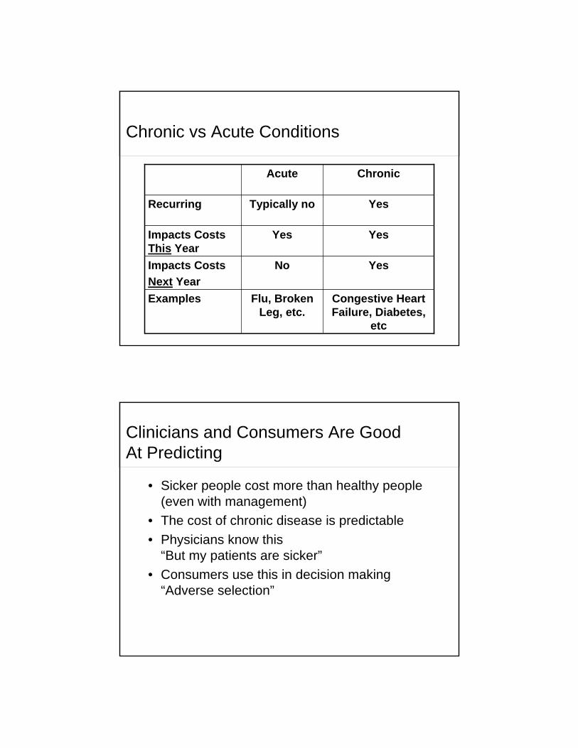
Chronic vs Acute Conditions

Congestive Heart Failure, Diabetes,

etc

Flu, Broken Leg, etc.

Examples

YesNoImpacts CostsNext Year

YesYesImpacts Costs This Year

YesTypically noRecurring

ChronicAcute

Clinicians and Consumers Are Good At Predicting

• Sicker people cost more than healthy people (even with management)

• The cost of chronic disease is predictable• Physicians know this

“But my patients are sicker”• Consumers use this in decision making

“Adverse selection”

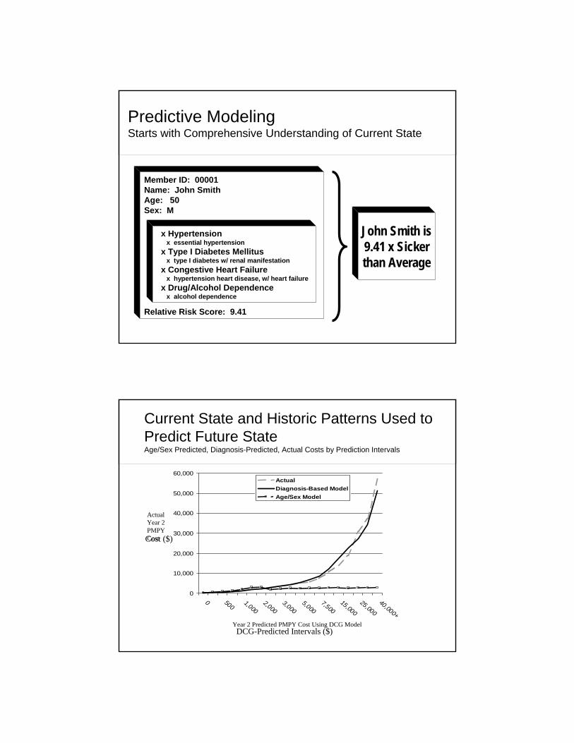
Member ID: 00001Name: John SmithAge: 50Sex: M

Relative Risk Score: 9.41

x Hypertensionx essential hypertension

x Type I Diabetes Mellitusx type I diabetes w/ renal manifestation

x Congestive Heart Failurex hypertension heart disease, w/ heart failure

x Drug/Alcohol Dependencex alcohol dependence

John Smith is9.41 x Sicker than Average

Predictive ModelingStarts with Comprehensive Understanding of Current State

Current State and Historic Patterns Used to Predict Future StateAge/Sex Predicted, Diagnosis-Predicted, Actual Costs by Prediction Intervals

0

10,000

20,000

30,000

40,000

50,000

60,000

0 5001,000

2,0003,000

5,0007,500

15,00025,000

40,000+

ActualDiagnosis-Based ModelAge/Sex Model

Cost ($)

DCG-Predicted Intervals ($)

Actual Year 2 PMPY Cost

Year 2 Predicted PMPY Cost Using DCG Model

Predictive Modeling :From Medicare-funded Research ….

Medicare Modernization Act extends use of risk adjustment to Medicare Part D (Drug Benefit) as well as in Chronic Care Improvement Programs in Part B (traditional Medicare)

2004

Balance Budget Amendment (BBA) mandates risk adjustment for Medicare Part C (Medicare+Choice later renamed Medicare Advantage)

1997

Medicare observes younger healthier beneficiaries enrolling in Medicare HMOs, resulting in higher costs Medicare funds several teams to develop alternative models to quantify impact of illness burden on expected costs

Congress enables Medicare beneficiaries to enroll in HMOs1982

…to Commercial Uses in Group Health

• Risk adjustment predictive modeling• Risk transfer payments

– Underwriting renewals High cost case identification

– Prioritization for disease/care management– Outcomes (ROI) analysis of cost

containment programs– Physician incentive programs

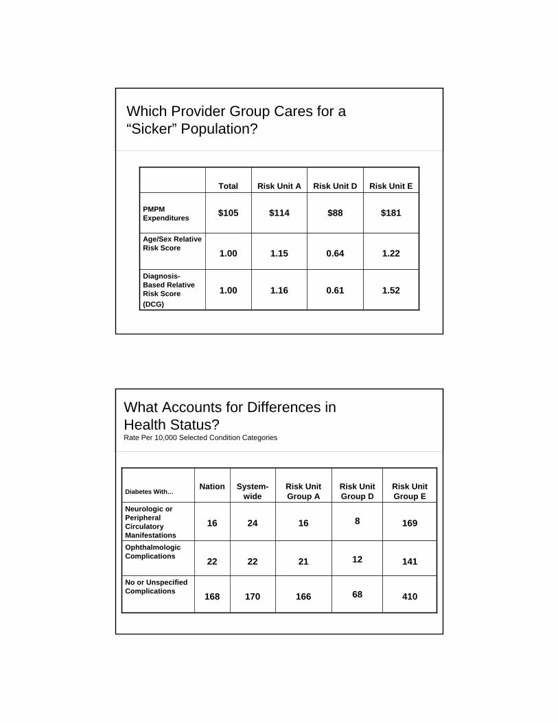
Which Provider Group Cares for a “Sicker” Population?

1.520.611.161.00Diagnosis-Based Relative Risk Score(DCG)

1.220.641.151.00Age/Sex Relative Risk Score

$181$88$114$105PMPM Expenditures

Risk Unit ERisk Unit DRisk Unit ATotal

What Accounts for Differences in Health Status?Rate Per 10,000 Selected Condition Categories

168

22

16

Nation

41068166170No or Unspecified Complications

141122122Ophthalmologic Complications

16981624Neurologic or Peripheral Circulatory Manifestations

Risk Unit Group E

Risk Unit Group D

Risk Unit Group A

System-wideDiabetes With…

Is Membership Growing “Sicker” Over Time ? (1.00 is mean risk using pharmacy-based models)

1997 2000

Continuing Enrollees (N=201, 049) New Enrollees

.80

.921.02 1.07

.45

.55

.69

Using Predictive Modeling for Reinsurance: Client Finding

• For small and mid-sized groups (up to 249 members), diagnosis-based models outperformed prior year costs at all retention levels

• For high retentions ($100K+), diagnosis-based models generally outperformed prior year costs

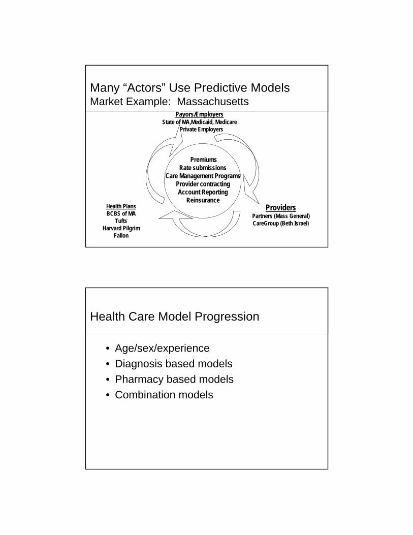
Many “Actors” Use Predictive Models Market Example: Massachusetts

Payors/EmployersState of MA,Medicaid, Medicare

Private Employers

ProvidersPartners (Mass General)CareGroup (Beth Israel)

Health PlansBCBS of MA

TuftsHarvard Pilgrim

Fallon

PremiumsRate submissions

Care Management ProgramsProvider contractingAccount Reporting

Reinsurance

Health Care Model Progression

• Age/sex/experience• Diagnosis based models • Pharmacy based models• Combination models

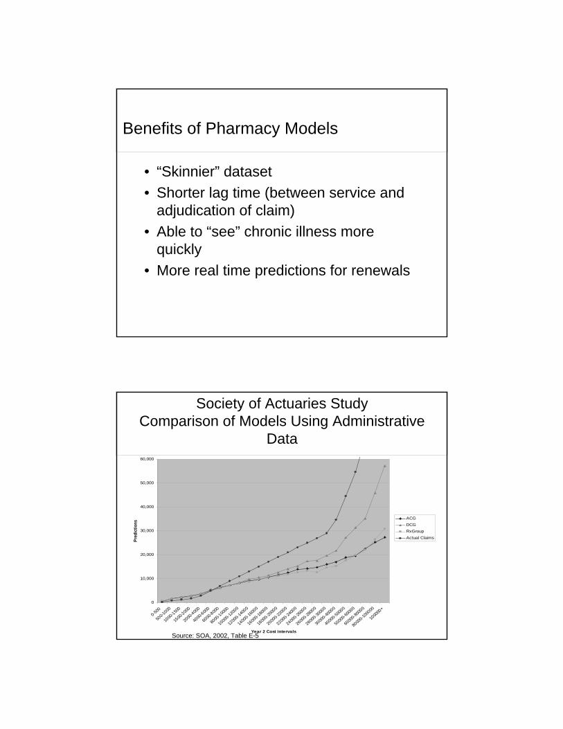
Benefits of Pharmacy Models

• “Skinnier” dataset• Shorter lag time (between service and

adjudication of claim)• Able to “see” chronic illness more

quickly• More real time predictions for renewals

Source: SOA, 2002, Table E-5

0

10,000

20,000

30,000

40,000

50,000

60,000

0-500

500-1

000

1000

-1500

1500

-2000

2000

-4000

4000

-6000

6000

-8000

8000

-10000

1000

0-120

00

1200

0-140

00

1400

0-160

00

1600

0-180

00

1800

0-200

00

2000

0-220

00

2200

0-240

00

2400

0-260

00

2600

0-280

00

2800

0-300

00

3000

0-400

00

4000

0-500

00

5000

0-600

00

6000

0-800

00

8000

0-100

000

1000

00+

Year 2 Cost intervals

Pred

ictio

ns

ACGDCGRxGroupActual Claims

Society of Actuaries Study Comparison of Models Using Administrative

Data

Beyond Administrative Data

• Health risk assessments/surveys• Lifestyle issues• Lab values • Biometric findings• Genetic markers

Why Group Health Models May Be Helpful in Workers Comp

• Small percentage of cases account for large % of claim costs

• Comordibities appear to influence costs• Proactive case management approach

has positive outcomes• Data classification and management

needed to build successful models

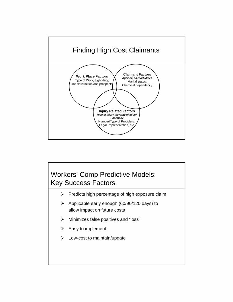
Finding High Cost Claimants

Work Place FactorsType of Work, Light duty,

Job satisfaction and prospects

Claimant FactorsAge/sex, co-morbidities

Marital status,Chemical dependency

Injury Related FactorsType of injury, severity of injury,

PharmacyNumber/Type of Providers, Legal Representation, etc.

Workers’ Comp Predictive Models: Key Success Factors

Predicts high percentage of high exposure claim

Applicable early enough (60/90/120 days) to allow impact on future costs

Minimizes false positives and “loss”

Easy to implement

Low-cost to maintain/update