cs281b/stat241b. statistical learning theory. lecture 7.bartlett/courses/2014spring-cs281... ·...
TRANSCRIPT

CS281B/Stat241B. Statistical Learning Theory. Lecture 7.Peter Bartlett
1. Uniform laws of large numbers
(a) Glivenko-Cantelli theorem proof:
Concentration. Symmetrization. Restrictions.
(b) Symmetrization: Rademacher complexity.
(c) Restrictions: growth function, VC dimension, ...
1
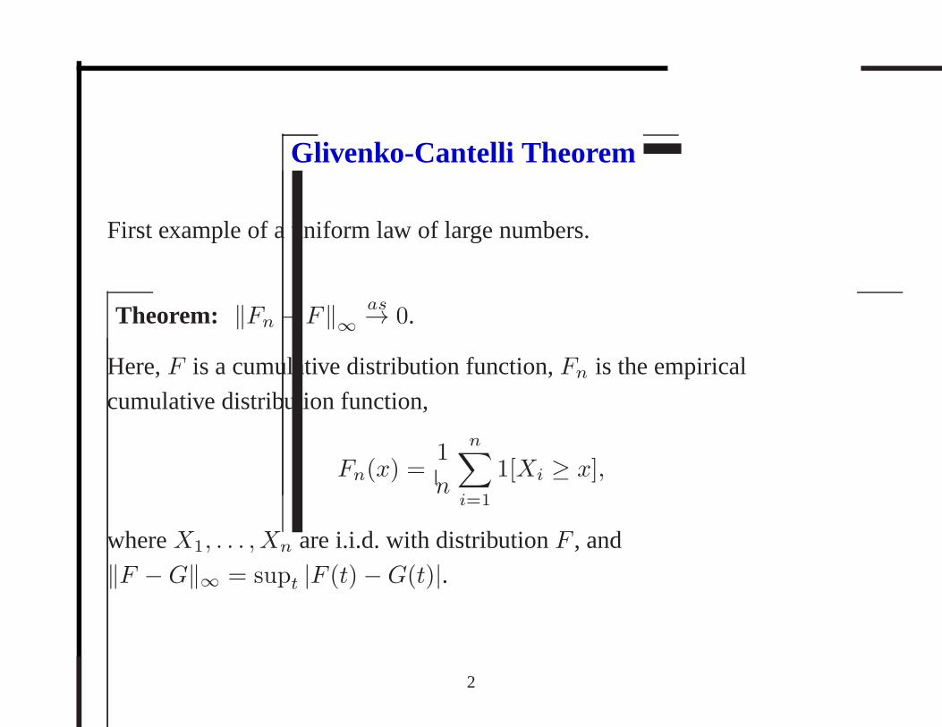
Glivenko-Cantelli Theorem
First example of a uniform law of large numbers.
Theorem: ‖Fn − F‖∞
as→ 0.
Here,F is a cumulative distribution function,Fn is the empirical
cumulative distribution function,
Fn(x) =1
n
n∑
i=1
1[Xi ≥ x],
whereX1, . . . , Xn are i.i.d. with distributionF , and
‖F −G‖∞ = supt |F (t)−G(t)|.
2

Proof of Glivenko-Cantelli Theorem
Theorem: ‖Fn − F‖∞
as→ 0.
That is,‖P − Pn‖G as→ 0, whereG = {x 7→ 1[x ≥ t] : t ∈ R}.
We’ll look at a proof that we’ll then extend to a more general sufficientcondition for a class to be Glivenko-Cantelli.
The proof involves three steps:
1. Concentration: with probability at least1− exp(−2ǫ2n),
‖P − Pn‖G ≤ E‖P − Pn‖G + ǫ.
2. Symmetrization:E‖P − Pn‖G ≤ 2E‖Rn‖G, where we’ve definedtheRademacher processRn(g) = (1/n)
∑ni=1 ǫig(Xi) (and this
leads us to consider restrictions of step functionsg ∈ G to the data),
3. Simple restrictions.
3
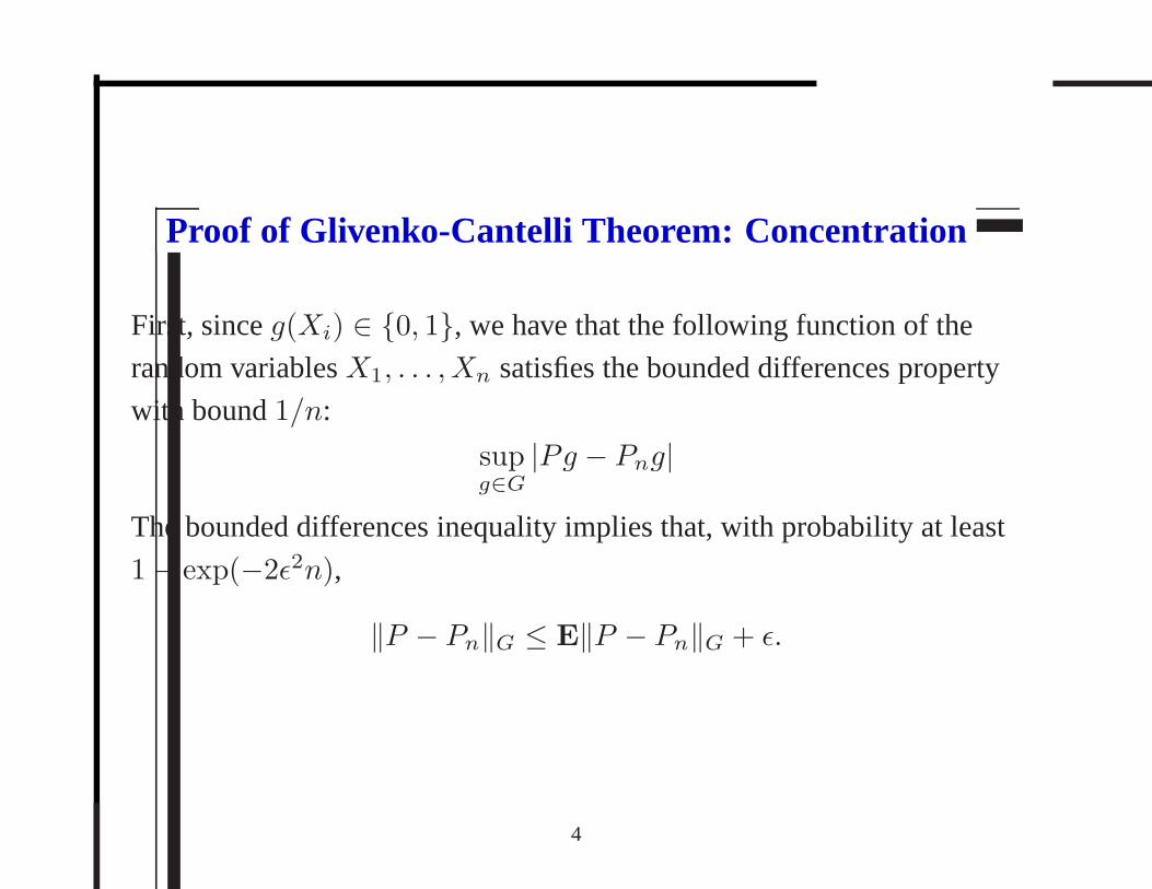
Proof of Glivenko-Cantelli Theorem: Concentration
First, sinceg(Xi) ∈ {0, 1}, we have that the following function of the
random variablesX1, . . . , Xn satisfies the bounded differences property
with bound1/n:
supg∈G
|Pg − Png|
The bounded differences inequality implies that, with probability at least
1− exp(−2ǫ2n),
‖P − Pn‖G ≤ E‖P − Pn‖G + ǫ.
4

Proof of Glivenko-Cantelli Theorem: Symmetrization
Second, we symmetrize by replacingPg by P ′ng = 1
n
∑ni=1 g(X
′i). In
particular, we have
E‖P − Pn‖G ≤ E‖P ′n − Pn‖G.
[Why?]
5

Proof of Glivenko-Cantelli Theorem: Symmetrization
Now we symmetrize again: for anyǫi ∈ {±1},
E supg∈G
∣∣∣∣∣
1
n
n∑
i=1
(g(X ′i)− g(Xi))
∣∣∣∣∣= E sup
g∈G
∣∣∣∣∣
1
n
n∑
i=1
ǫi(g(X′i)− g(Xi))
∣∣∣∣∣,
This follows from the fact thatXi andX ′i are i.i.d., and so the distribution
of the supremum is unchanged when we swap them. And so in particular
the expectation of the supremum is unchanged. And since thisis true for
anyǫi, we can take the expectation over any random choice of theǫi.
We’ll pick them independently and uniformly.
6

Proof of Glivenko-Cantelli Theorem: Symmetrization
E supg∈G
∣∣∣∣∣
1
n
n∑
i=1
ǫi(g(X′i)− g(Xi))
∣∣∣∣∣
≤ E supg∈G
∣∣∣∣∣
1
n
n∑
i=1
ǫig(X′i)
∣∣∣∣∣+ sup
g∈G
∣∣∣∣∣
1
n
n∑
i=1
ǫig(Xi)
∣∣∣∣∣
≤ 2E supg∈G
∣∣∣∣∣
1
n
n∑
i=1
ǫig(Xi)
∣∣∣∣∣
︸ ︷︷ ︸
Rademacher complexity
= 2E‖Rn‖G,
where we’ve defined theRademacher processRn(g) = (1/n)
∑n
i=1 ǫig(Xi).
7

Proof of Glivenko-Cantelli Theorem: Restrictions
We consider the set of restrictions
G(Xn1 ) = {(g(X1), . . . , g(Xn)) : g ∈ G}:
2E‖Rn‖G = 2E supg∈G
∣∣∣∣∣
1
n
n∑
i=1
ǫig(Xi)
∣∣∣∣∣= 2EE
[
supg∈G
∣∣∣∣∣
1
n
n∑
i=1
ǫig(Xi)
∣∣∣∣∣
∣∣∣∣∣Xn
1
]
.
But notice that the cardinality ofG(Xn1 ) does not change if we order the
data. That is,
|G((X1, . . . , Xn))| =∣∣G((X(1), . . . , X(n)))
∣∣
=∣∣{(1[X(1) ≥ t], . . . , 1[X(n) ≥ t]) : t ∈ R
}∣∣ ≤ n+ 1,
whereX(1) ≤ · · · ≤ X(n) is the data in sorted order (and soX(i) ≥ t
impliesX(i+1) ≥ t).
8
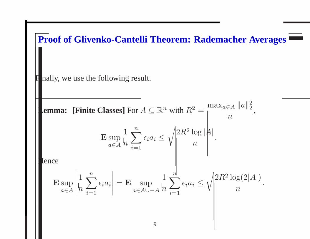
Proof of Glivenko-Cantelli Theorem: Rademacher Averages
Finally, we use the following result.
Lemma: [Finite Classes]ForA ⊆ Rn with R2 =
maxa∈A ‖a‖22n
,
E supa∈A
1
n
n∑
i=1
ǫiai ≤√
2R2 log |A|n
.
Hence
E supa∈A
∣∣∣∣∣
1
n
n∑
i=1
ǫiai
∣∣∣∣∣= E sup
a∈A∪−A
1
n
n∑
i=1
ǫiai ≤√
2R2 log(2|A|)n
.
9
Proof of Rademacher Averages Result
10

Proof of Glivenko-Cantelli Theorem
For the classG of step functions,R ≤ 1/√n and|A| ≤ n+1. Thus, with
probability at least1− exp(−2ǫ2n),
‖P − Pn‖G ≤√
8 log(2(n+ 1))
n+ ǫ.
By Borel-Cantelli,‖P − Pn‖G as→ 0.
11
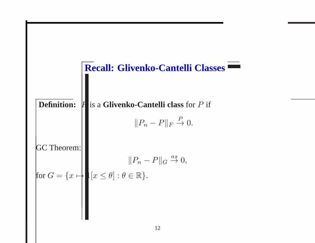
Recall: Glivenko-Cantelli Classes
Definition: F is aGlivenko-Cantelli classfor P if
‖Pn − P‖F P→ 0.
GC Theorem:
‖Pn − P‖G as→ 0,
for G = {x 7→ 1[x ≤ θ] : θ ∈ R}.
12

Uniform laws and Rademacher complexity
The proof of the Glivenko-Cantelli Theorem involved three steps:
1. Concentration of‖P − Pn‖F about its expectation.
2. Symmetrization, which boundsE‖P − Pn‖F in terms of the
Rademacher complexity ofF , E‖Rn‖F .
3. A combinatorial argument showing that the set of restrictions ofF to
Xn1 is small, and a bound on theRademacher complexityusing this
fact.
We’ll follow a similar path to prove a more general uniform law of large
numbers.
13

Uniform laws and Rademacher complexity
Definition: The Rademacher complexityof F is E‖Rn‖F , where the
empirical processRn is defined as
Rn(f) =1
n
n∑
i=1
ǫif(Xi),
where theǫ1, . . . , ǫn are Rademacher random variables: i.i.d. uniform on
{±1}.
Note that this is the expected supremum of the alignment between the
random{±1}-vectorǫ andF (Xn1 ), the set ofn-vectors obtained by
restrictingF to the sampleX1, . . . , Xn.
14

Uniform laws and Rademacher complexity
Theorem: For anyF , E‖P − Pn‖F ≤ 2E‖Rn‖F .
If F ⊂ [0, 1]X ,
1
2E‖Rn‖F −
√
log 2
2n≤ E‖P − Pn‖F ≤ 2E‖Rn‖F ,
and, with probability at least1− 2 exp(−2ǫ2n),
E‖P − Pn‖F − ǫ ≤ ‖P − Pn‖F ≤ E‖P − Pn‖F + ǫ.
Thus,E‖Rn‖F → 0 iff ‖P − Pn‖F as→ 0.
That is, the sup of the empirical processP − Pn is concentrated about its
expectation, and its expectation is about the same as the expected sup of
the Rademacher processRn.
15
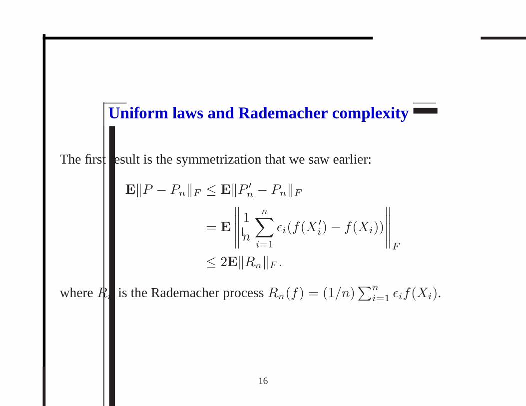
Uniform laws and Rademacher complexity
The first result is the symmetrization that we saw earlier:
E‖P − Pn‖F ≤ E‖P ′n − Pn‖F
= E
∥∥∥∥∥
1
n
n∑
i=1
ǫi(f(X′i)− f(Xi))
∥∥∥∥∥F
≤ 2E‖Rn‖F .
whereRn is the Rademacher processRn(f) = (1/n)∑n
i=1 ǫif(Xi).
16
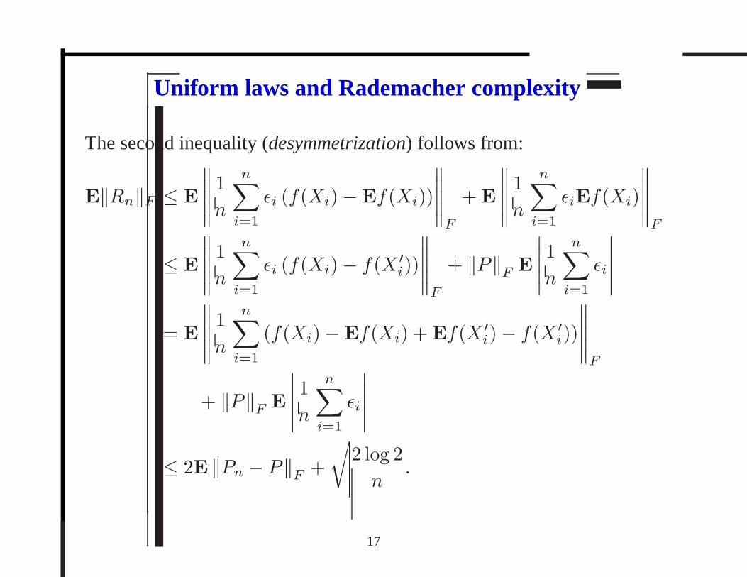
Uniform laws and Rademacher complexity
The second inequality (desymmetrization) follows from:
E‖Rn‖F ≤ E
∥∥∥∥∥
1
n
n∑
i=1
ǫi (f(Xi)−Ef(Xi))
∥∥∥∥∥F
+E
∥∥∥∥∥
1
n
n∑
i=1
ǫiEf(Xi)
∥∥∥∥∥F
≤ E
∥∥∥∥∥
1
n
n∑
i=1
ǫi (f(Xi)− f(X ′i))
∥∥∥∥∥F
+ ‖P‖F E
∣∣∣∣∣
1
n
n∑
i=1
ǫi
∣∣∣∣∣
= E
∥∥∥∥∥
1
n
n∑
i=1
(f(Xi)−Ef(Xi) +Ef(X ′i)− f(X ′
i))
∥∥∥∥∥F
+ ‖P‖F E
∣∣∣∣∣
1
n
n∑
i=1
ǫi
∣∣∣∣∣
≤ 2E ‖Pn − P‖F +
√
2 log 2
n.
17
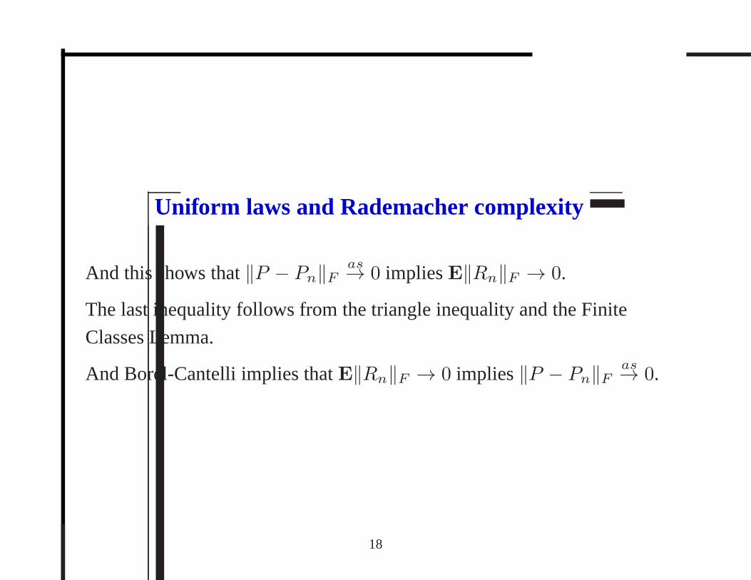
Uniform laws and Rademacher complexity
And this shows that‖P − Pn‖F as→ 0 impliesE‖Rn‖F → 0.
The last inequality follows from the triangle inequality and the Finite
Classes Lemma.
And Borel-Cantelli implies thatE‖Rn‖F → 0 implies‖P − Pn‖F as→ 0.
18
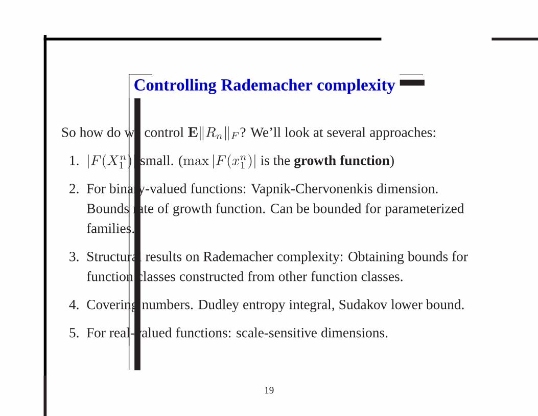
Controlling Rademacher complexity
So how do we controlE‖Rn‖F? We’ll look at several approaches:
1. |F (Xn1 )| small. (max |F (xn
1 )| is thegrowth function )
2. For binary-valued functions: Vapnik-Chervonenkis dimension.
Bounds rate of growth function. Can be bounded for parameterized
families.
3. Structural results on Rademacher complexity: Obtainingbounds for
function classes constructed from other function classes.
4. Covering numbers. Dudley entropy integral, Sudakov lower bound.
5. For real-valued functions: scale-sensitive dimensions.
19
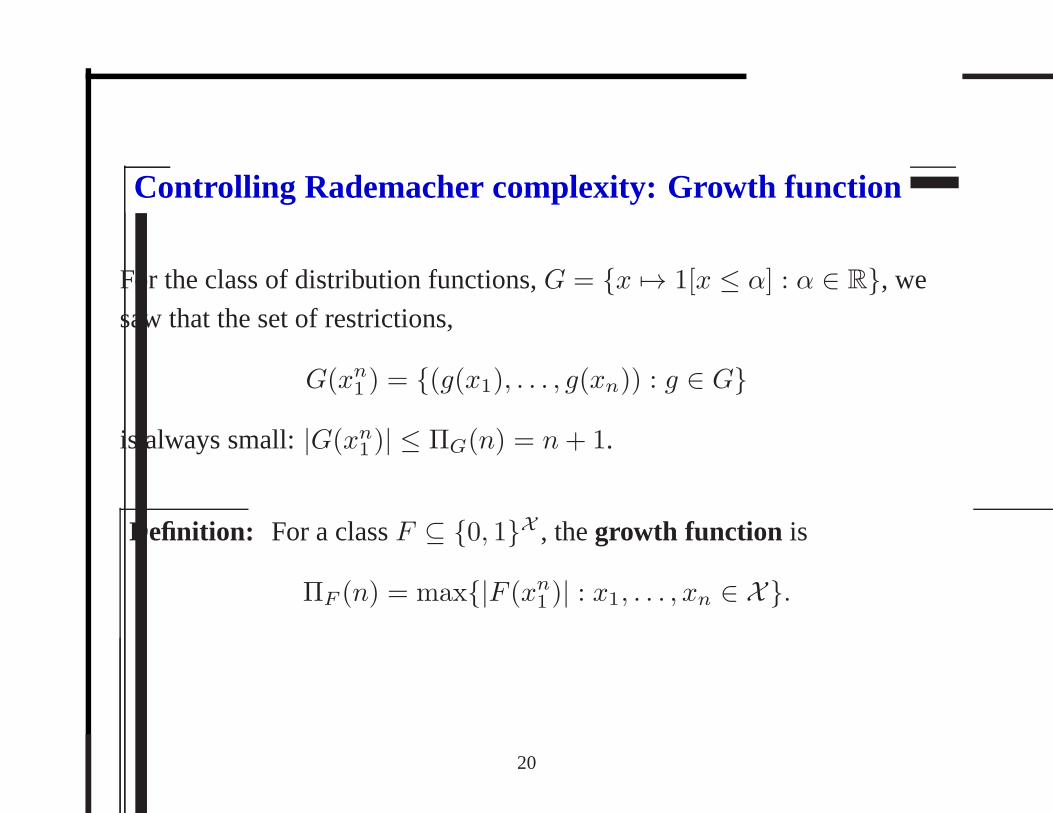
Controlling Rademacher complexity: Growth function
For the class of distribution functions,G = {x 7→ 1[x ≤ α] : α ∈ R}, we
saw that the set of restrictions,
G(xn1 ) = {(g(x1), . . . , g(xn)) : g ∈ G}
is always small:|G(xn1 )| ≤ ΠG(n) = n+ 1.
Definition: For a classF ⊆ {0, 1}X , thegrowth function is
ΠF (n) = max{|F (xn1 )| : x1, . . . , xn ∈ X}.
20

Controlling Rademacher complexity: Growth function
Lemma: [Finite Class Lemma] Forf ∈ F satisfying|f(x)| ≤ 1,
E‖Rn‖F ≤ E
√
2 log(|F (Xn1 ) ∪ −F (Xn
1 )|)n
≤√
2 log(2E|F (Xn1 )|)
n.
[whereRn is the Rademacher process:
Rn(f) =1
n
n∑
i=1
ǫif(Xi).
andF (Xn1 ) is the set of restrictions of functions inF toX1, . . . , Xn.]
21
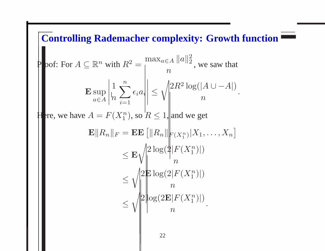
Controlling Rademacher complexity: Growth function
Proof: ForA ⊆ Rn with R2 =
maxa∈A ‖a‖22n
, we saw that
E supa∈A
∣∣∣∣∣
1
n
n∑
i=1
ǫiai
∣∣∣∣∣≤
√
2R2 log(|A ∪ −A|)n
.
Here, we haveA = F (Xn1 ), soR ≤ 1, and we get
E‖Rn‖F = EE[‖Rn‖F (Xn
1)|X1, . . . , Xn
]
≤ E
√
2 log(2|F (Xn1 )|)
n
≤√
2E log(2|F (Xn1 )|)
n
≤√
2 log(2E|F (Xn1 )|)
n.
22

Controlling Rademacher complexity: Growth function
e.g. For the class of distribution functions,G = {x 7→ 1[x ≥ α] : α ∈ R},
we saw that|G(xn1 )| ≤ n+ 1. SoE‖Rn‖F ≤
√2 log 2(n+1)
n.
e.g.F parameterized byk bits:
If g maps to[0, 1],
F ={x 7→ g(x, θ) : θ ∈ {0, 1}k
},
|F (xn1 )| ≤ 2k,
E‖Rn‖F ≤√
2(k + 1) log 2
n.
Notice thatE‖Rn‖F → 0.
23
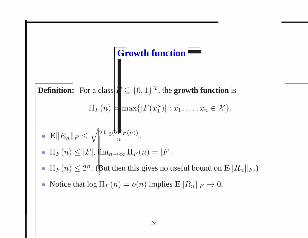
Growth function
Definition: For a classF ⊆ {0, 1}X , thegrowth function is
ΠF (n) = max{|F (xn1 )| : x1, . . . , xn ∈ X}.
• E‖Rn‖F ≤√
2 log(2ΠF (n))n
.
• ΠF (n) ≤ |F |, limn→∞ ΠF (n) = |F |.
• ΠF (n) ≤ 2n. (But then this gives no useful bound onE‖Rn‖F .)
• Notice thatlog ΠF (n) = o(n) impliesE‖Rn‖F → 0.
24
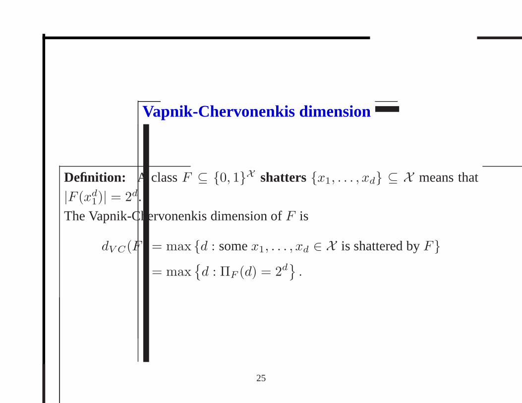
Vapnik-Chervonenkis dimension
Definition: A classF ⊆ {0, 1}X shatters{x1, . . . , xd} ⊆ X means that
|F (xd1)| = 2d.
The Vapnik-Chervonenkis dimension ofF is
dV C(F ) = max {d : somex1, . . . , xd ∈ X is shattered byF}= max
{d : ΠF (d) = 2d
}.
25
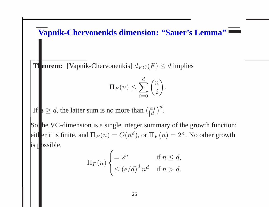
Vapnik-Chervonenkis dimension: “Sauer’s Lemma”
Theorem: [Vapnik-Chervonenkis]dV C(F ) ≤ d implies
ΠF (n) ≤d∑
i=0
(n
i
)
.
If n ≥ d, the latter sum is no more than(end
)d.
So the VC-dimension is a single integer summary of the growthfunction:
either it is finite, andΠF (n) = O(nd), orΠF (n) = 2n. No other growth
is possible.
ΠF (n)
= 2n if n ≤ d,
≤ (e/d)dnd if n > d.
26

Vapnik-Chervonenkis dimension: “Sauer’s Lemma”
Thus, fordV C(F ) ≤ d andn ≥ d, we have
E‖Rn‖F ≤√
2 log(2ΠF (n))
n≤
√
2 log 2 + 2d log(en/d)
n.
27