CS294-6Reconfigurable Computing

Day 6

September 10, 1998

Comparing Computing Devices

Today

• Finish up empirical comparisons

• Instructions and their impact

• Modeling

Multiply

FIR

IIR/Biquad

DES Keysearch

<http://www.cs.berkeley.edu/~iang/isaac/hardware/>

DNA Sequence Match

• Problem: “cost” of transform S1S2

• Given: cost of insertion, deletion, substitution

• Relevance: similarity of DNA sequences– evolutionary similarity– structure predict function

• Typically: new sequence compared to large databse

DNA Sequence Match

Floating-Point Add (single prec.)

Floating-Point Mpy (single prec.)

Summary

• Raw densities (Area-Time)– FPGA/custom = 100x– Processor/custom = 1000x

• Special-purpose functional units in processors/DSPs, much lower net benefit since need to control and interconnect

• Gap narrows (closes) as programmable can be specialized

Modeling

• Why do we model?

Terminology

• Primitive Instruction (pinst)– Collection of bits which tell a bit-processing

element what to do– Includes:

• select compute operation

• input sources in space (interconnect)

• input sources in time (retiming)

Computational Array Model

• Collection of computing elements– compute operator

– local storage/retiming

• Interconnect• Instruction

“Ideal” Instruction Control

• Issue a new instruction to every computational bit operator on every cycle

“Ideal” Instruction Distribution

• Why don’t we do this?

“Ideal” Instruction Distribution

• Problem: Instruction bandwidth (and storage area) quickly dominates everything else– Compute Block ~ 1M x– Instruction ~ 64 bits– Wire Pitch ~ – Memory bit ~

Instruction Distribution64

x8=

512

Tw

o in

stru

ctio

ns in

102

4

Instruction Distribution

Distribute from both sides = 2x

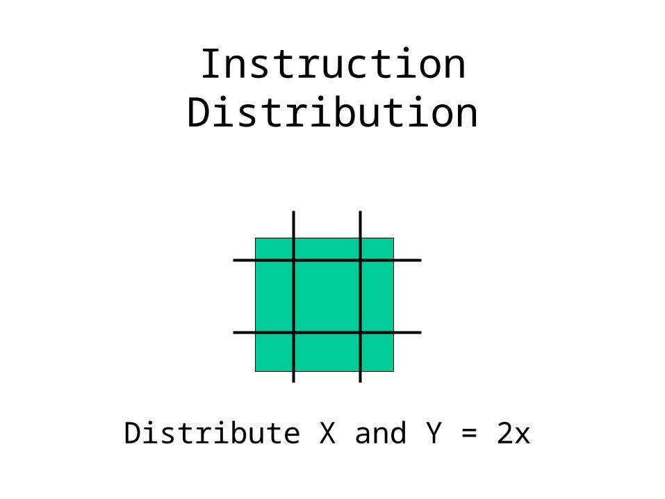
Instruction Distribution

Distribute X and Y = 2x

Instruction Distribution

• Room to distribute 2 instructions across PE per metal layer (1024 = 2x8x64)

• Feed top and bottom (left and right) = 2x

• Two complete metal layers = 2x

• => 8 instructions / PE Side

Instruction Distribution

• Maximum of 8 instructions per PE side

• Saturate wire channels at 8xN = N

• => at 64 PE– beyond this instruction distribution dominates

area

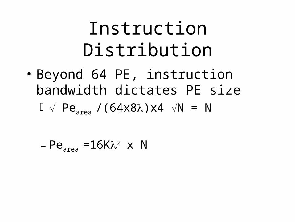
Instruction Distribution

• Beyond 64 PE, instruction bandwidth dictates PE size Pearea /(64x8)x4 N = N

– Pearea =16K x N

Instruction Memory Requirements

• Idea: put instruction memory in array

• Problem: Instruction memory can quickly dominate area, too– Memory Area = 64x1.2K/instruction

– PEarea = 1M+ (Instructions)x80K

Instruction Pragmatics

• Instruction requirements could dominate array size.

• Standard architecture trick:– Look for structure to exploit in “typical

computations”

Typical Structure?

• What structure do we usually expect?

Two Extremes

• SIMD Array (microprocessors)– Instruction/cycle

– share instruction across array of PE s

– uniform operation in space

– operation variance in time

• FPGA– Instruction/PE

– assume temporal locality of instructions (same)

– operation variance in space

– uniform operations in time

Hybrids

• VLIW (SuperScalar)– Few pinsts/cycle– Share instruction across w bits

• DPGA– Small instruction store / PE

Architecture Instr. Taxonomy

Modeling Instruction Effects

• Restrictions from “ideal” save area

• Restriction from “ideal” limits usability (yield) of PE

• Want to understand effects– area model– utilization/yield model

Efficiency/Yield Intuition

• What happens when– Datapath is too wide?– Datapath is too narrow?– Instruction memory is too deep?– Instruction memory is too shallow?

Computing Device

• Composition– Bit Processing

elements

– Interconnect• space

• time

– Instruction Memory

Computing Device Composition

• Tile basic building blocks into array

Model Area

Spot Check Area• FPGA

– w=1, d=c=1, k=4 880K

– Xilinx 4K 630K

– Altera 8K 930K

• SIMD– w=1000, c-0, d-64, k=3 170K

– Abacus 190K

• Processor– w=32, d=32, c=1024, k=2 2.6M

– MIPS-X 2.1M

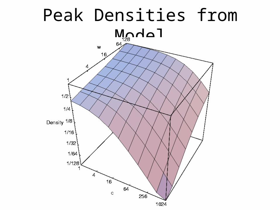
Peak Densities from Model

Empirical Peak Densities

Efficiency

• What do we want to maximize?– Useful work per unit silicon

• Yield Fraction / Area

• (or minimize (Area/Yield) )

Efficiency

• For comparison, look at relative efficiency to ideal.

• Ideal = architecture exactly matched to application requirements

• Efficiency = Aideal/Aarch

• Aarch = Area Op/Yield

Efficiency Calculation

Efficiency with fixed Width

w=1,16K PEs

FPGA vs. DPGA Compare

Robust point: when context memory area is 1/2 of total area

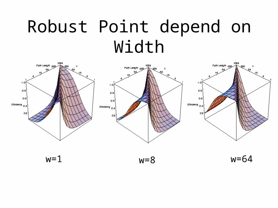
Robust Point depend on Width

w=1 w=8 w=64

Processors and FPGAs

FPGAc=d=1, w=1, k=4

“Processor”c=d=1024, w=64, k=2

Intermediate Architecture

w=8 c=6416K PEs

Caveats

• Model abstracts away many details which are important– interconnect– control– specialized functional units

• Applications are a heterogeneous mix of characteristics

Modeling Message

• Architecture space is huge

• Easy to be very inefficient

• Hard to pick one point robust across entire space

Summary

• Instruction resources can be significant• Exploit application structure to reduce

instruction requirements• Classify architectures by instruction

organization• Arch. structure and application requirements

mismatch => inefficiencies• Model => visualize efficiency trends