CS344 : Introduction to Artificial Intelligence

Pushpak BhattacharyyaCSE Dept., IIT Bombay

Lecture 30: Computing power of Perceptron;

Perceptron Training

Perceptron

recap

The Perceptron Model

A perceptron is a computing element with input lines having associated weights and the cell having a threshold value. The perceptron model is motivated by the biological neuron.

Output = y

wnWn-1

w1

Xn-1

x1

Threshold = θ

Computation of Boolean functions

AND of 2 inputsX1 x2 y0 0 00 1 01 0 01 1 1The parameter values (weights & thresholds) need to be found.

y

w1 w2

x1 x2

θ

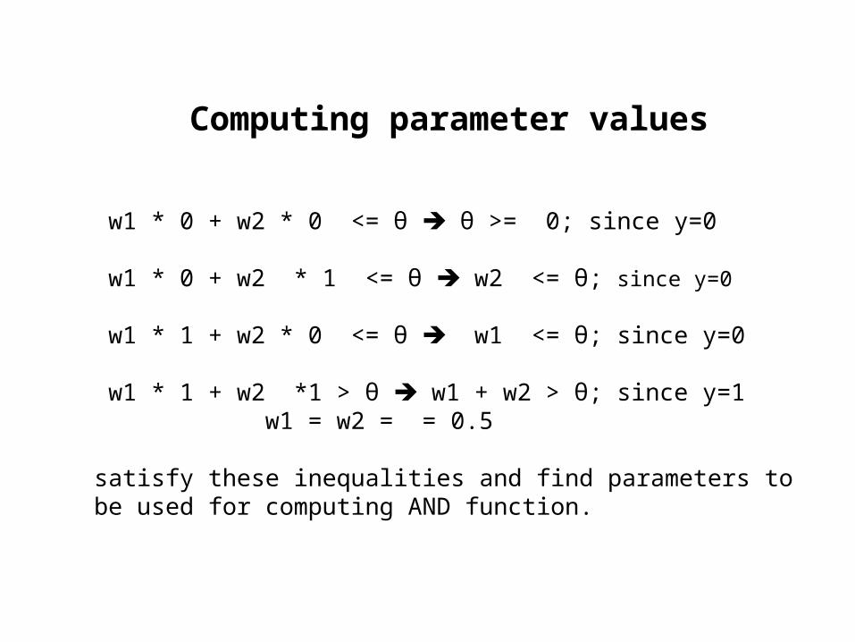
Computing parameter values

w1 * 0 + w2 * 0 <= θ θ >= 0; since y=0

w1 * 0 + w2 * 1 <= θ w2 <= θ; since y=0

w1 * 1 + w2 * 0 <= θ w1 <= θ; since y=0

w1 * 1 + w2 *1 > θ w1 + w2 > θ; since y=1w1 = w2 = = 0.5

satisfy these inequalities and find parameters to be used for computing AND function.

Threshold functions

n # Boolean functions (2^2^n) #Threshold Functions (2n2)

1 4 42 16 143 256 1284 64K 1008

• Functions computable by perceptrons - threshold functions

• #TF becomes negligibly small for larger values of #BF.

• For n=2, all functions except XOR and XNOR are computable.

Concept of Hyper-planes

• ∑ wixi = θ defines a linear surface in the (W,θ) space, where W=<w1,w2,w3,…,wn> is an n-dimensional vector.

• A point in this (W,θ) space

defines a perceptron.

y

x1

. . .

θ

w1 w2 w3 wn

x2 x3 xn

Simple perceptron contd.

10101

11000

f4f3f2f1x

θ≥0w≤θ

θ≥0w> θ

θ<0w≤ θ

θ<0W< θ

0-function Identity Function Complement Function

True-Function

Counting the number of functions for the simplest perceptron

• For the simplest perceptron, the equation is w.x=θ.

Substituting x=0 and x=1,

we get θ=0 and w=θ.

These two lines intersect to

form four regions, which

correspond to the four functions.

θ=0

w=θ

R1

R2R3

R4

θ

w

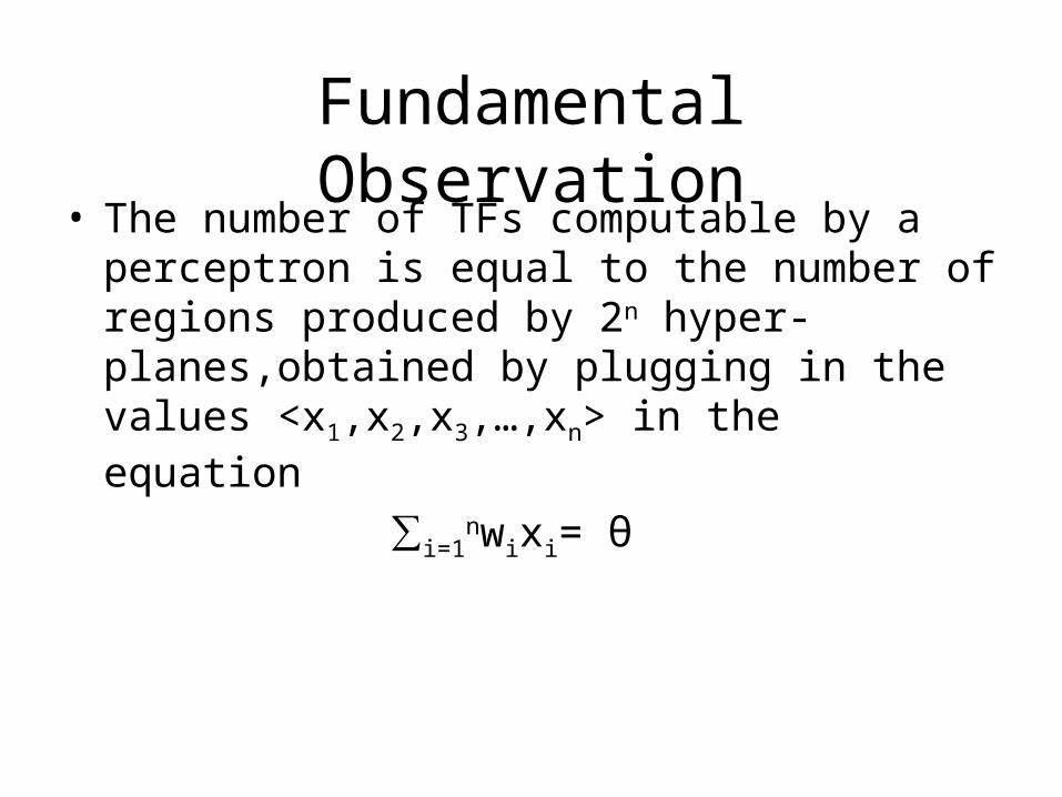
Fundamental Observation• The number of TFs computable by a perceptron is

equal to the number of regions produced by 2n hyper-planes,obtained by plugging in the values <x1,x2,x3,…,xn> in the equation

∑i=1nwixi= θ

For 2 input perceptron

• Basic equation

• w1x1+w2x2-θ=0

• Put 4 values of x1 and x2: <0,0>, <0,1>, <1,0>, <1,1>

• Defines 4 planes through the origin of the <w1, w2, θ>

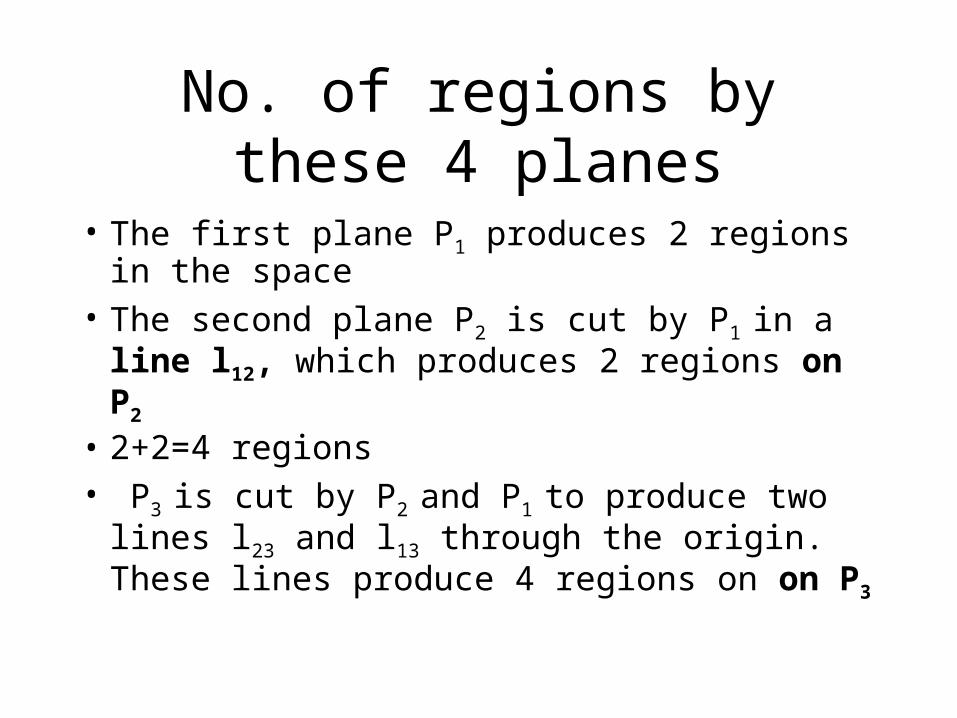
No. of regions by these 4 planes

• The first plane P1 produces 2 regions in the space

• The second plane P2 is cut by P1 in a line l12, which produces 2 regions on P2

• 2+2=4 regions• P3 is cut by P2 and P1 to produce two lines

l23 and l13 through the origin. These lines produce 4 regions on on P3

No. of regions (contd.)

• 4+4= 8 regions when P3 is introduced

• P4 is cut by P1, P2, P3 to produce 3 lines passing through origin and producing 6 regions on P4

• Total no. of regions= 8+6=14

• This is the no. of Boolean functions that 2-input perceptron will be able to compute

Perceptron Training Algorithm

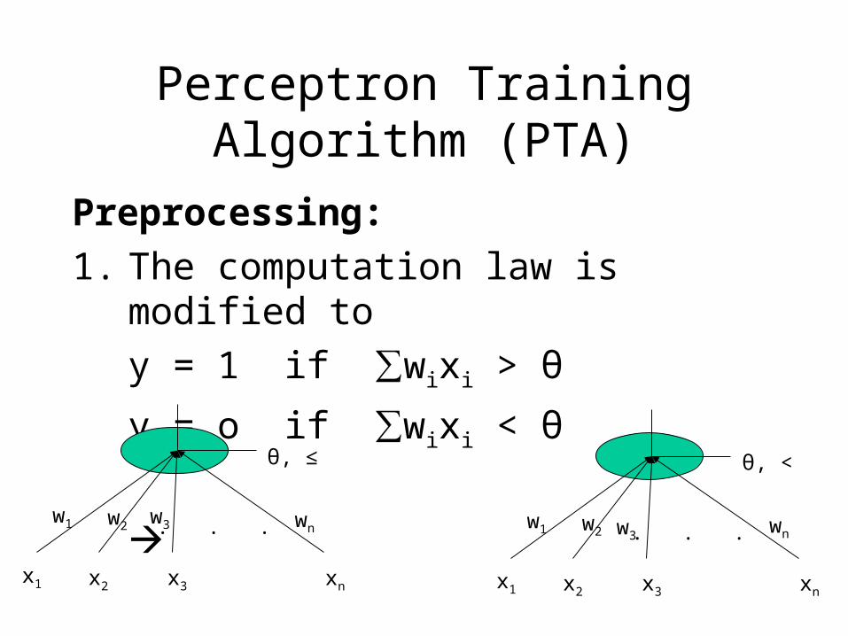
Perceptron Training Algorithm (PTA)

Preprocessing:

1. The computation law is modified to

y = 1 if ∑wixi > θ

y = o if ∑wixi < θ

. . .

θ, ≤

w1 w2 wn

x1 x2 x3 xn

. . .

θ, <

w1 w2 w3wn

x1 x2 x3 xn

w3

PTA – preprocessing cont…

2. Absorb θ as a weight

3. Negate all the zero-class examples

. . .

θ

w1 w2 w3 wn

x2 x3 xnx1

w0=θ

x0= -1

. . .

θ

w1 w2 w

3

wn

x2 x3 xnx1

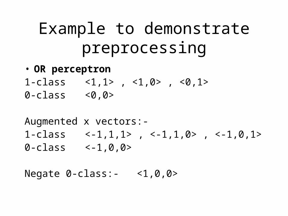
Example to demonstrate preprocessing

• OR perceptron1-class <1,1> , <1,0> , <0,1>0-class <0,0>

Augmented x vectors:-1-class <-1,1,1> , <-1,1,0> , <-1,0,1>0-class <-1,0,0>

Negate 0-class:- <1,0,0>

Example to demonstrate preprocessing cont..

Now the vectors are

x0 x1 x2

X1 -1 0 1

X2 -1 1 0

X3 -1 1 1

X4 1 0 0

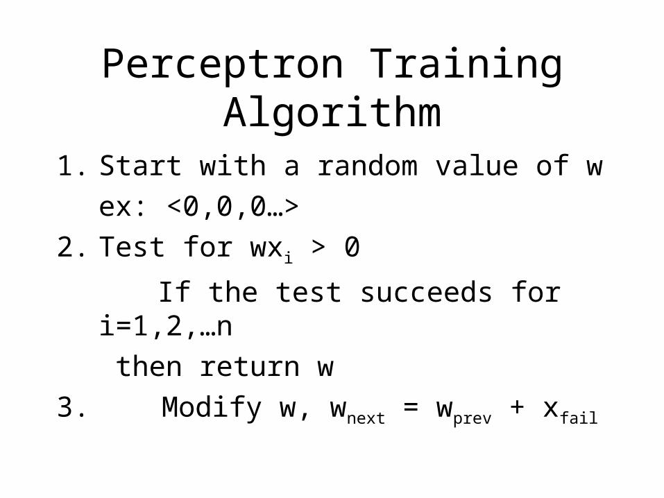
Perceptron Training Algorithm

1. Start with a random value of w

ex: <0,0,0…>

2. Test for wxi > 0

If the test succeeds for i=1,2,…n

then return w

3. Modify w, wnext = wprev + xfail

Tracing PTA on OR-example

w=<0,0,0> wx1 fails

w=<-1,0,1> wx4 fails

w=<0,0 ,1> wx2 fails

w=<-1,1,1> wx1 fails

w=<0,1,2> wx4 fails

w=<1,1,2> wx2 fails

w=<0,2,2> wx4 fails w=<1,2,2> success

Proof of Convergence of PTA

• Perceptron Training Algorithm (PTA)

• Statement:

Whatever be the initial choice of weights and whatever be the vector chosen for testing, PTA converges if the vectors are from a linearly separable function.

Proof of Convergence of PTA

• Suppose wn is the weight vector at the nth step of the algorithm.

• At the beginning, the weight vector is w0

• Go from wi to wi+1 when a vector Xj fails the test wiXj > 0 and update wi as

wi+1 = wi + Xj

• Since Xjs form a linearly separable function, w* s.t. w*Xj > 0 j

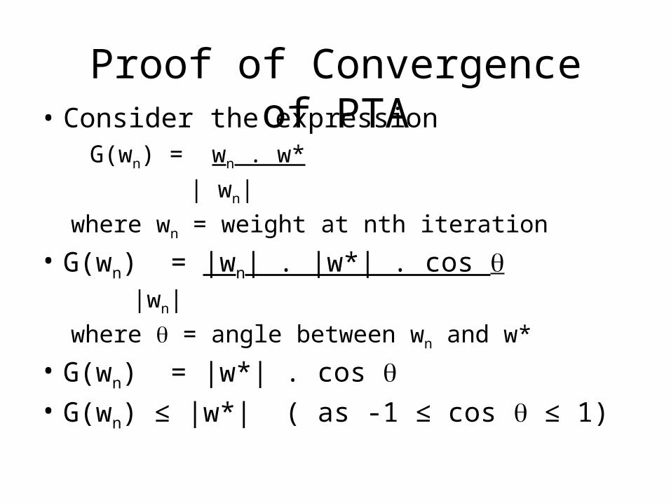
Proof of Convergence of PTA• Consider the expression

G(wn) = wn . w*

| wn|

where wn = weight at nth iteration

• G(wn) = |wn| . |w*| . cos |wn|

where = angle between wn and w*

• G(wn) = |w*| . cos • G(wn) ≤ |w*| ( as -1 ≤ cos ≤ 1)

Behavior of Numerator of Gwn . w* = (wn-1 + Xn-1

fail ) . w*wn-1 . w* + Xn-1

fail . w* (wn-2 + Xn-2

fail ) . w* + Xn-1fail . w* …..

w0 . w* + ( X0fail + X1

fail +.... + Xn-1fail ). w*

w*.Xifail is always positive: note carefully

• Suppose |Xj| ≥ , where is the minimum magnitude.

• Num of G ≥ |w0 . w*| + n . |w*| • So, numerator of G grows with n.

Behavior of Denominator of G

• |wn| = wn . wn

(wn-1 + Xn-1fail )2

(wn-1)2 + 2. wn-1. Xn-1

fail + (Xn-1fail )2

≤ (wn-1)2 + (Xn-1

fail )2 (as wn-1. Xn-1

fail ≤ 0 )

≤ (w0)2 + (X0

fail )2 + (X1fail )2 +…. + (Xn-1

fail )2

• |Xj| ≤ (max magnitude)

• So, Denom ≤ (w0)2 + n2

Some Observations

• Numerator of G grows as n

• Denominator of G grows as n

=> Numerator grows faster than denominator

• If PTA does not terminate, G(wn) values will become unbounded.

Some Observations contd.

• But, as |G(wn)| ≤ |w*| which is finite, this is impossible!

• Hence, PTA has to converge.

• Proof is due to Marvin Minsky.

Convergence of PTA

•Whatever be the initial choice of weights and whatever be the vector chosen for testing, PTA converges if the vectors are from a linearly separable function.