CS347 – Introduction toArtificial Intelligence

Dr. Daniel Tauritz (Dr. T)Department of Computer Science

tauritzd@mst.eduhttp://web.mst.edu/~tauritzd/

CS347 course website: http://web.mst.edu/~tauritzd/courses/cs347/

What is AI?

Systems that…–act like humans (Turing Test)–think like humans–think rationally–act rationally

Play Ultimatum Game

Key historical events for AI• 4th century BC Aristotle propositional logic• 1600’s Descartes mind-body connection• 1805 First programmable machine• Mid 1800’s Charles Babbage’s “difference

engine” & “analytical engine”• Lady Lovelace’s Objection• 1847 George Boole propositional logic• 1879 Gottlob Frege predicate logic

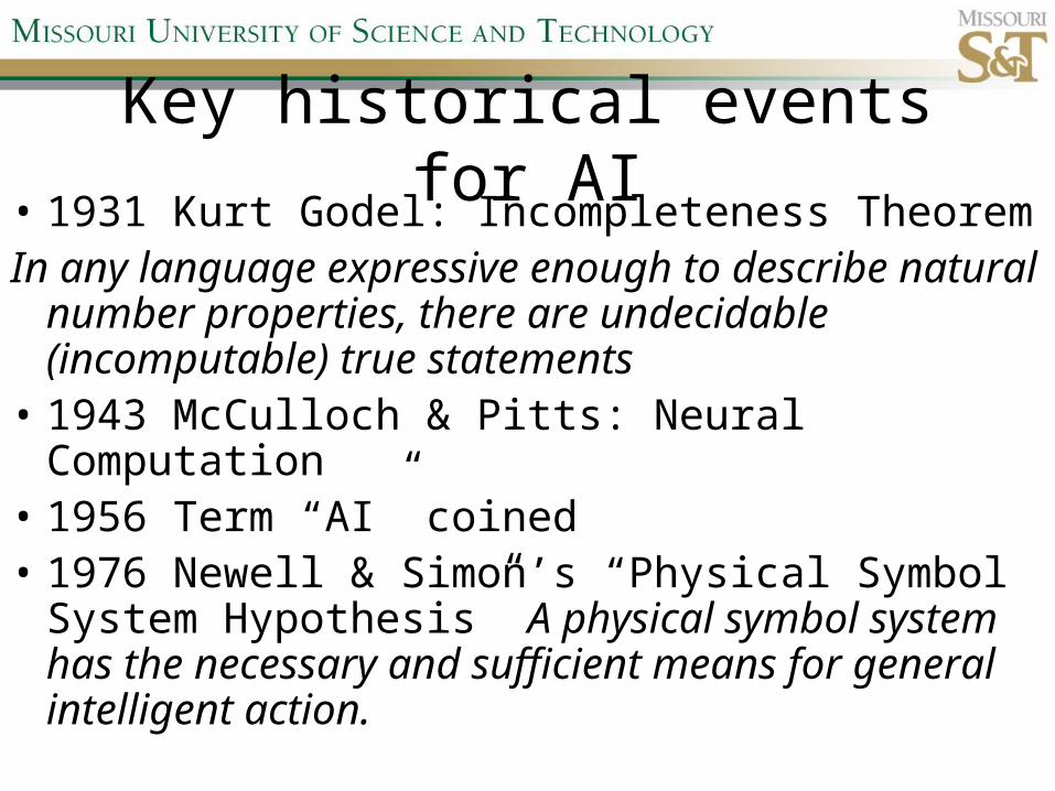
Key historical events for AI• 1931 Kurt Godel: Incompleteness TheoremIn any language expressive enough to describe

natural number properties, there are undecidable (incomputable) true statements

• 1943 McCulloch & Pitts: Neural Computation• 1956 Term “AI” coined• 1976 Newell & Simon’s “Physical Symbol

System Hypothesis” A physical symbol system has the necessary and sufficient means for general intelligent action.

How difficult is it to achieve AI?

• Three Sisters Puzzle

Rational Agents

• Environment• Sensors (percepts)• Actuators (actions)• Agent Function• Agent Program• Performance Measures

Rational Behavior

Depends on:

• Agent’s performance measure

• Agent’s prior knowledge

• Possible percepts and actions

• Agent’s percept sequence

Rational Agent Definition

“For each possible percept sequence, a rational agent selects an action that is expected to maximize its performance measure, given the evidence provided by the percept sequence and any prior knowledge the agent has.”

Task EnvironmentsPEAS description & properties:

–Fully/Partially Observable–Deterministic, Stochastic, Strategic–Episodic, Sequential–Static, Dynamic, Semi-dynamic–Discrete, Continuous–Single agent, Multiagent–Competitive, Cooperative

Problem-solving agents

A definition:

Problem-solving agents are goal based agents that decide what to do based on an action sequence leading to a goal state.

Problem-solving steps

• Problem-formulation

• Goal-formulation

• Search

• Execute solution

Well-defined problems

• Initial state• Successor function• Goal test• Path cost• Solution• Optimal solution

Example problems

• Vacuum world

• Tic-tac-toe

• 8-puzzle

• 8-queens problem

Search trees• Root corresponds with initial state• Vacuum state space vs. search tree• Search algorithms iterate through goal

testing and expanding a state until goal found

• Order of state expansion is critical!• Water jug example

Search node datastructure

• STATE• PARENT-NODE• ACTION• PATH-COST• DEPTH

States are NOT search nodes!

Fringe

• Fringe = Set of leaf nodes

• Implemented as a queue with ops:– MAKE-QUEUE(element,…)– EMPTY?(queue)– FIRST(queue)– REMOVE-FIRST(queue)– INSERT(element,queue)– INSERT-ALL(elements,queue)

Problem-solving performance

• Completeness

• Optimality

• Time complexity

• Space complexity

Complexity in AI• b – branching factor• d – depth of shallowest goal node• m – max path length in state space• Time complexity: # generated nodes• Space complexity: max # nodes stored• Search cost: time + space complexity• Total cost: search + path cost

Tree Search• Breadth First Tree Search (BFTS)

• Uniform Cost Tree Search (UCTS)

• Depth-First Tree Search (DFTS)

• Depth-Limited Tree Search (DLTS)

• Iterative-Deepening Depth-First Tree Search (ID-DFTS)

Graph Search• Breadth First Graph Search (BFGS)

• Uniform Cost Graph Search (UCGS)

• Depth-First Graph Search (DFGS)

• Depth-Limited Graph Search (DLGS)

• Iterative-Deepening Depth-First Graph Search (ID-DFGS)

Example state space

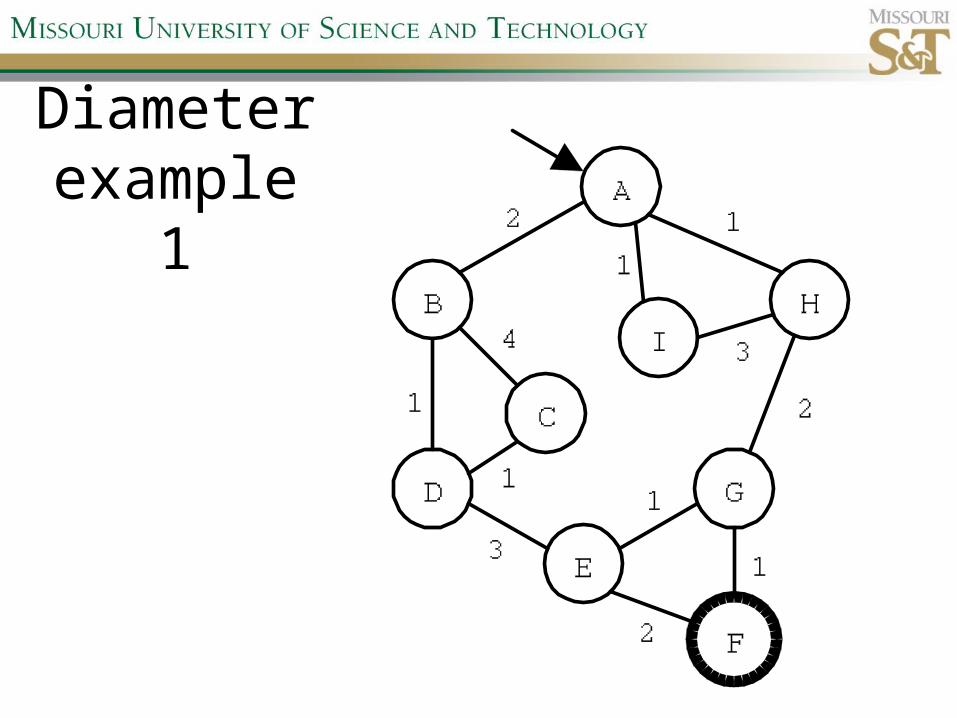
Diameter example 1

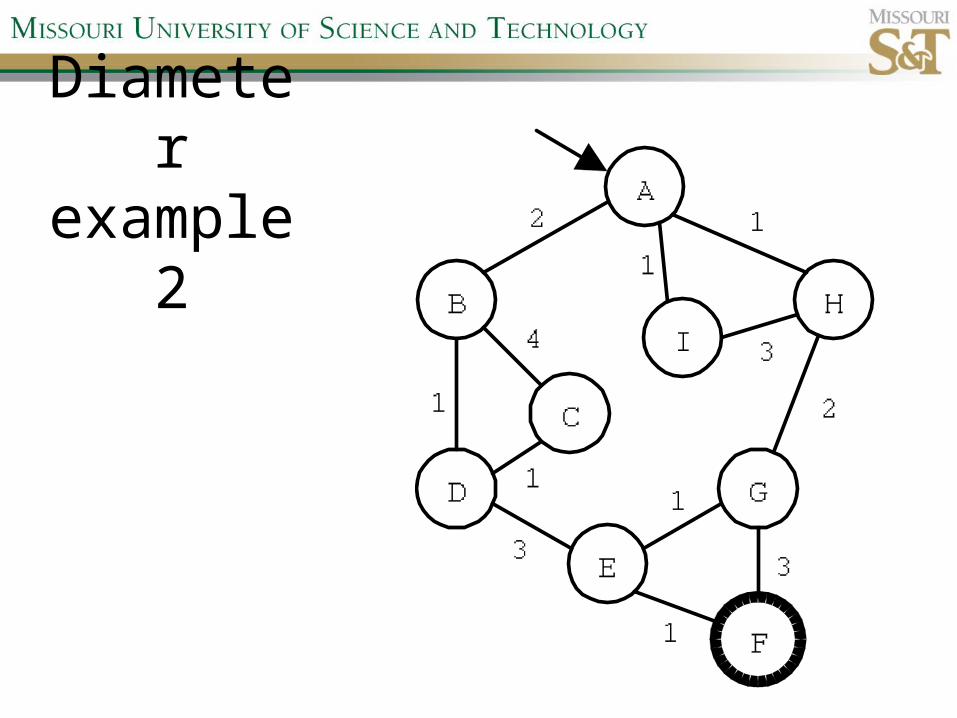
Diameter example 2

Best First Search (BeFS)• Select node to expand based on

evaluation function f(n)

• Typically node with lowest f(n) selected because f(n) correlated with path-cost

• Represent fringe with priority queue sorted in ascending order of f-values

Path-cost functions

• g(n) = lowest path-cost from start node to node n

• h(n) = estimated path-cost of cheapest path from node n to a goal node [with h(goal)=0]

Important BeFS algorithms

• UCS: f(n) = g(n)

• GBeFS: f(n) = h(n)

• A*S: f(n) = g(n)+h(n)

Heuristics

• h(n) is a heuristic function

• Heuristics incorporate problem-specific knowledge

• Heuristics need to be relatively efficient to compute

GBeFS

• Incomplete (so also not optimal)

• Worst-case time and space complexity: O(bm)

• Actual complexity depends on accuracy of h(n)

A*S

• f(n) = g(n) + h(n)

• f(n): estimated cost of optimal solution through node n

• if h(n) satisfies certain conditions, A*S is complete & optimal

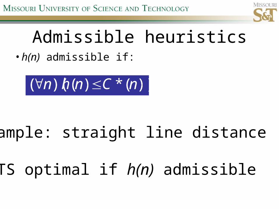
Admissible heuristics• h(n) admissible if:

Example: straight line distance

A*TS optimal if h(n) admissible

Consistent heuristics• h(n) consistent if:

Consistency implies admissibility

A*GS optimal if h(n) consistent

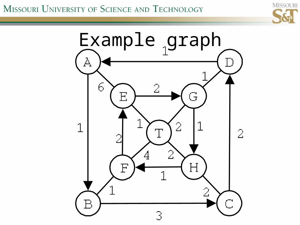
Example graph

Local Search

• Steepest-ascent hill-climbing• Stochastic hill-climbing• First-choice hill-climbing• Random-restart hill-climbing• Simulated Annealing• Deterministic local beam search• Stochastic local beam search• Evolutionary Algorithms

Adversarial SearchEnvironments characterized by:• Competitive multi-agent• Turn-taking

Simplest type: Discrete, deterministic, two-player, zero-sum games of perfect information

Search problem formulation• Initial state: board position & starting

player• Successor function: returns list of

(legal move, state) pairs• Terminal test: game over!• Utility function: associates player-

dependent values with terminal states

Minimax

Depth-Limited Minimax• State Evaluation Heuristic

estimates Minimax value of a node

• Note that the Minimax value of a node is always calculated for the Max player, even when the Min player is at move in that node!

Iterative-Deepening Minimax• IDM(n,d) calls DLM(n,1), DLM(n,2),

…, DLM(n,d)• Advantages:

–Solution availability when time is critical

–Guiding information for deeper searches

Redundant info example

Alpha-Beta Pruning• α: worst value that Max will accept at this

point of the search tree

• β: worst value that Min will accept at this point of the search tree

• Fail-low: encountered value <= α

• Fail-high: encountered value >= β

• Prune if fail-low for Min-player

• Prune if fail-high for Max-player

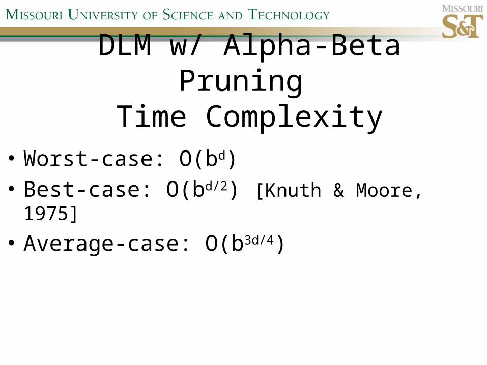
DLM w/ Alpha-Beta Pruning Time Complexity

• Worst-case: O(bd)• Best-case: O(bd/2) [Knuth & Moore, 1975]

• Average-case: O(b3d/4)

Move Ordering Heuristics

• Knowledge based

• Killer Move: the last move at a given depth that caused an AB-pruning or had best minimax value

• History Table

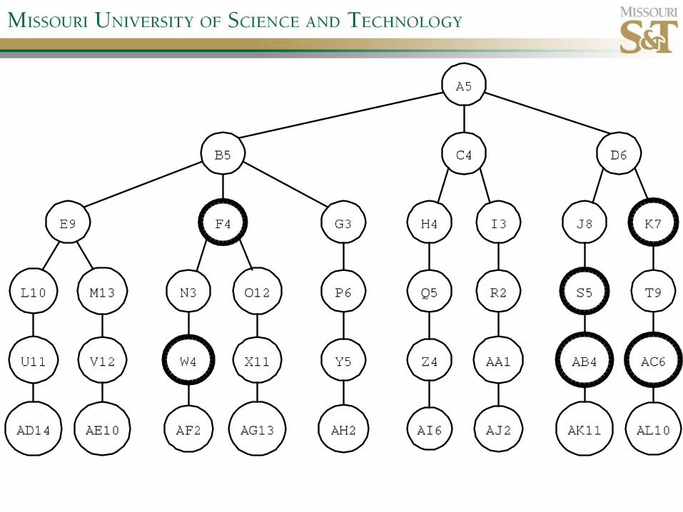
Example game tree

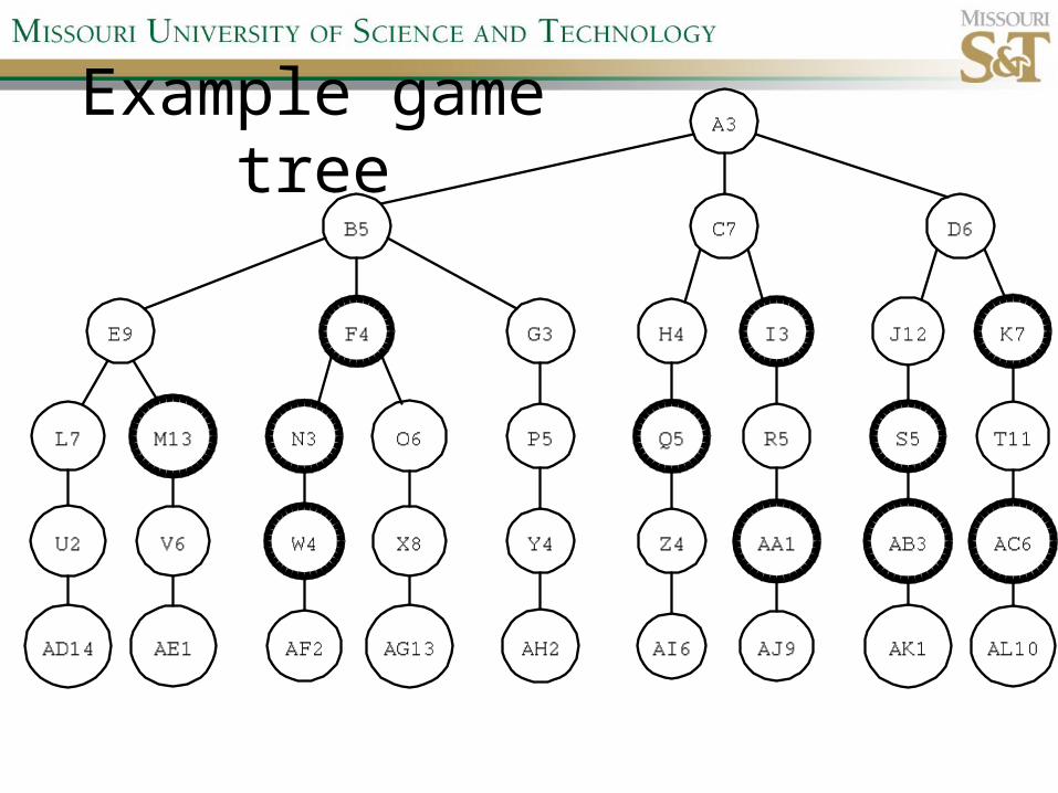
Example game tree

Example game tree

Search Depth Heuristics• Time based / State based

• Horizon Effect: the phenomenon of deciding on a non-optimal principal variant because an ultimately unavoidable damaging move seems to be avoided by blocking it till passed the search depth

• Singular Extensions / Quiescence Search

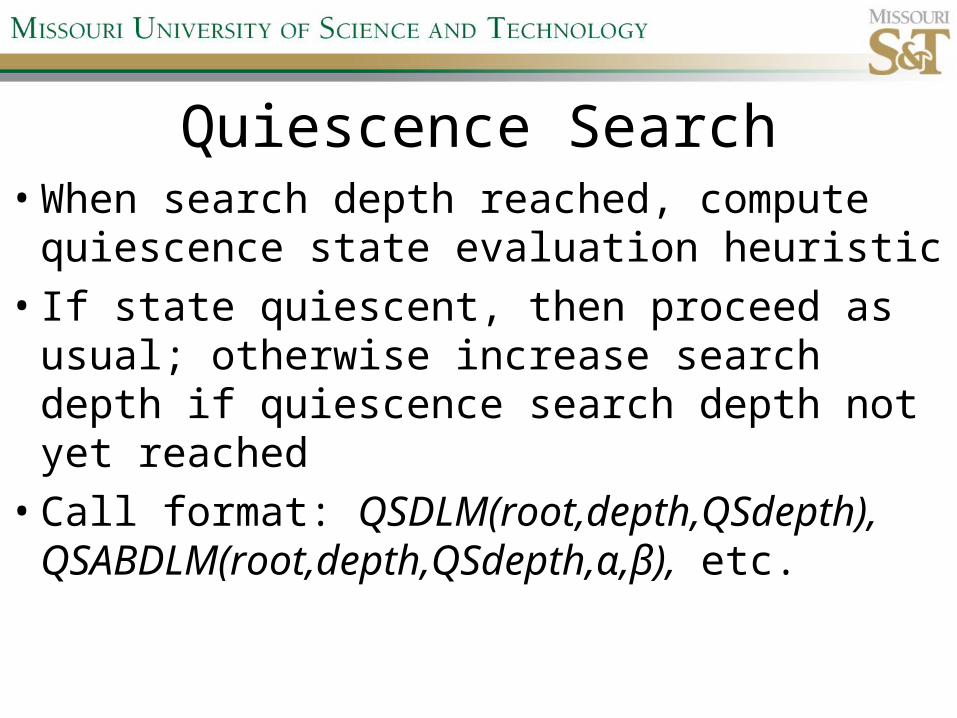
Quiescence Search• When search depth reached, compute

quiescence state evaluation heuristic

• If state quiescent, then proceed as usual; otherwise increase search depth if quiescence search depth not yet reached

• Call format: QSDLM(root,depth,QSdepth), QSABDLM(root,depth,QSdepth,α,β), etc.

Time Per Move

• Constant

• Percentage of remaining time

• State dependent

• Hybrid

Transposition Tables (1)

• Hash table of previously calculated state evaluation heuristic values

• Speedup is particularly huge for iterative deepening search algorithms!

• Good for chess because often repeated states in same search

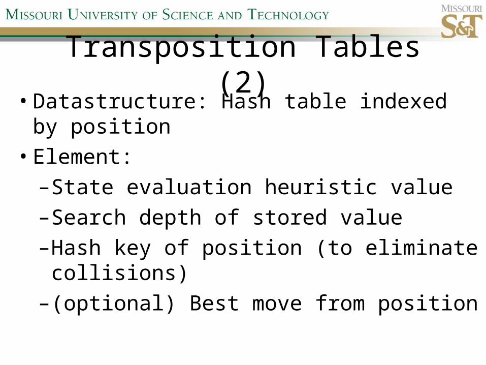
Transposition Tables (2)• Datastructure: Hash table indexed by

position

• Element:

–State evaluation heuristic value

–Search depth of stored value

–Hash key of position (to eliminate collisions)

–(optional) Best move from position

Transposition Tables (3)• Zobrist hash key

– Generate 3d-array of random 64-bit numbers (piece type, location and color)

– Start with a 64-bit hash key initialized to 0– Loop through current position, XOR’ing hash

key with Zobrist value of each piece found (note: once a key has been found, use an incremental apporach that XOR’s the “from” location and the “to” location to move a piece)

MTD(f)MTDf(root,guess,depth) {

lower = -∞;

upper = ∞;

do {

beta=guess+(guess==lower);

guess = ABMaxV(root,depth,beta-1,beta);

if (guess<beta) upper=guess; else lower=guess;

} while (lower < upper);

return guess; } // also needs to return best move

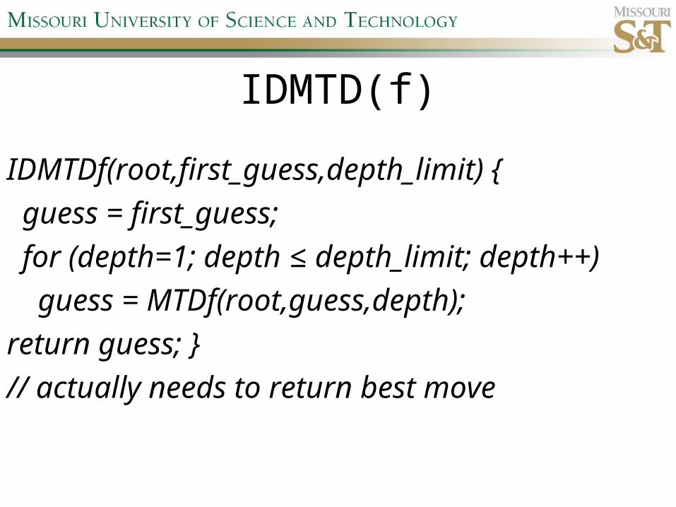
IDMTD(f)

IDMTDf(root,first_guess,depth_limit) {

guess = first_guess;

for (depth=1; depth ≤ depth_limit; depth++)

guess = MTDf(root,guess,depth);

return guess; }

// actually needs to return best move

Adversarial Search inStochastic Environments

Worst Case Time Complexity: O(bmnm) with b the average branching factor, m the deepest search depth, and n the average chance branching factor

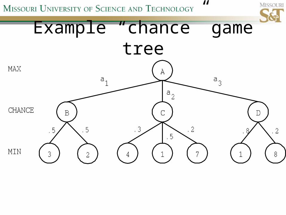
Example “chance” game tree

Expectiminimax & Pruning

• Interval arithmetic!

Null Move Forward Pruning

• Before regular search, perform shallower depth search (typically two ply less) with the opponent at move; if beta exceeded, then prune without performing regular search

• Sacrifices optimality for great speed increase

Futility Pruning

• If the current side to move is not in check, the current move about to be searched is not a capture and not a checking move, and the current positional score plus a certain margin (generally the score of a minor piece) would not improve alpha, then the current node is poor, and the last ply of searching can be aborted.

• Extended Futility Pruning

• Razoring

Online Search

• Offline search vs. online search

• Interleaving computation & action

• Exploration problems, safely explorable

• Agents have access to:– ACTIONS(s)– c(s,a,s’)– GOAL-TEST(s)

Online Search Optimality

• CR – Competitive Ratio

• TAPC – Total Actual Path Cost

• C* - Optimal Path Cost

• Best case: CR = 1

• Worst case: CR = ∞

*

TAPCCR

C

Online Search Algorithms

• Online-DFS-Agent

• Random Walk

• Learning Real-Time A* (LRTA*)

Online Search Example Graph

Particle Swarm Optimization

• PSO is a stochastic population-based optimization technique which assigns velocities to population members encoding trial solutions

• PSO update rules:

Ant Colony Optimization

• Population based

• Pheromone trail and stigmergetic communication

• Shortest path searching

• Stochastic moves