cs520: variable coefficients and nonlinear …ascher/520/chapt05.pdfcs520: variable coefficients and...
TRANSCRIPT
CS520: Variable coefficients and nonlinearproblems (Ch. 5)
Uri Ascher
Department of Computer ScienceUniversity of British Columbia
people.cs.ubc.ca/∼ascher/520.html
Uri Ascher (UBC) CPSC 520: Difference methods (Ch. 5) Fall 2012 1 / 51

Difference methods for PDEs
Outline
Freezing coefficients and dissipativity
Schemes for hyperbolic systems in 1D
Discontinuous solutions (Ch. 10)
Semi-Lagrangian methods
Nonlinear stability and energy method
Uri Ascher (UBC) CPSC 520: Difference methods (Ch. 5) Fall 2012 2 / 51
Difference methods for PDEs Dissipativity
Freezing coefficients
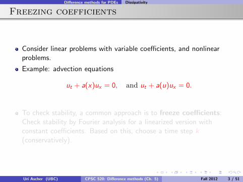
Consider linear problems with variable coefficients, and nonlinearproblems.
Example: advection equations
ut + a(x)ux = 0, and ut + a(u)ux = 0.
To check stability, a common approach is to freeze coefficients:Check stability by Fourier analysis for a linearized version withconstant coefficients. Based on this, choose a time step k(conservatively).
Uri Ascher (UBC) CPSC 520: Difference methods (Ch. 5) Fall 2012 3 / 51

Difference methods for PDEs Dissipativity
Freezing coefficients
Consider linear problems with variable coefficients, and nonlinearproblems.
Example: advection equations
ut + a(x)ux = 0, and ut + a(u)ux = 0.
To check stability, a common approach is to freeze coefficients:Check stability by Fourier analysis for a linearized version withconstant coefficients. Based on this, choose a time step k(conservatively).
Uri Ascher (UBC) CPSC 520: Difference methods (Ch. 5) Fall 2012 3 / 51
Difference methods for PDEs Dissipativity
Freezing coefficients cont.
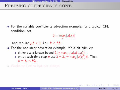
For the variable coefficients advection example, for a typical CFLcondition, set
a = maxx|a(x)|
and require µa < 1, i.e., k < ha.
For the nonlinear advection example, it’s a bit trickier:
either use a known bound a ≥ maxt,x |a(u(t, x))|,or, at each time step n use a = an = maxj |a(vn
j ))|. Thenk = kn < han.
Works well often but not always
Uri Ascher (UBC) CPSC 520: Difference methods (Ch. 5) Fall 2012 4 / 51

Difference methods for PDEs Dissipativity
Freezing coefficients cont.
For the variable coefficients advection example, for a typical CFLcondition, set
a = maxx|a(x)|
and require µa < 1, i.e., k < ha.
For the nonlinear advection example, it’s a bit trickier:
either use a known bound a ≥ maxt,x |a(u(t, x))|,or, at each time step n use a = an = maxj |a(vn
j ))|. Thenk = kn < han.
Works well often but not always
Uri Ascher (UBC) CPSC 520: Difference methods (Ch. 5) Fall 2012 4 / 51

Difference methods for PDEs Dissipativity
Example: Korteweg - de Vries (KdV)
A famous PDE: nonlinear, third derivative in x , admits solitonsolutions:
ut = α(u2)x + ρux + νuxxx
= [V ′(u)]x + νuxxx , V (u) =α
3u3 +
ρ
2u2.
Initial conditions u(0, x) = u0(x)
Boundary conditions: periodic
Set ρ = 0. Consider Eulerian finite volume/difference discretizations:on a fixed grid with step sizes k , h.
Uri Ascher (UBC) CPSC 520: Difference methods (Ch. 5) Fall 2012 5 / 51
Difference methods for PDEs Dissipativity
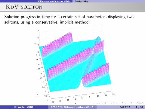
KdV soliton
Solution progress in time for a certain set of parameters displaying twosolitons, using a conservative, implicit method:
−20 −15 −10 −5 0 5 10 15 20
0
0.5
1
1.5
2
2.5
3
3.5
4
4.5
5
−5
0
5
10
x
t
u
Uri Ascher (UBC) CPSC 520: Difference methods (Ch. 5) Fall 2012 6 / 51

Difference methods for PDEs Dissipativity
Explicit numerical method
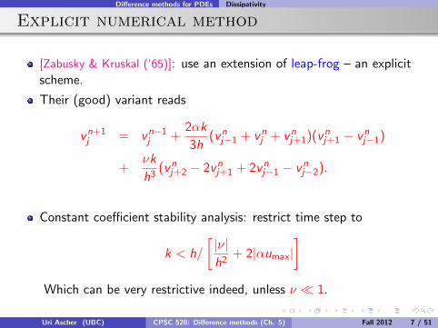
[Zabusky & Kruskal (’65)]: use an extension of leap-frog – an explicitscheme.
Their (good) variant reads
vn+1j = vn−1
j +2αk
3h(vn
j−1 + vnj + vn
j+1)(vnj+1 − vn
j−1)
+νk
h3(vn
j+2 − 2vnj+1 + 2vn
j−1 − vnj−2).
Constant coefficient stability analysis: restrict time step to
k < h/
[|ν|h2
+ 2|αumax|]
Which can be very restrictive indeed, unless ν � 1.
Uri Ascher (UBC) CPSC 520: Difference methods (Ch. 5) Fall 2012 7 / 51

Difference methods for PDEs Dissipativity
Explicit numerical method
[Zabusky & Kruskal (’65)]: use an extension of leap-frog – an explicitscheme.
Their (good) variant reads
vn+1j = vn−1
j +2αk
3h(vn
j−1 + vnj + vn
j+1)(vnj+1 − vn
j−1)
+νk
h3(vn
j+2 − 2vnj+1 + 2vn
j−1 − vnj−2).
Constant coefficient stability analysis: restrict time step to
k < h/
[|ν|h2
+ 2|αumax|]
Which can be very restrictive indeed, unless ν � 1.
Uri Ascher (UBC) CPSC 520: Difference methods (Ch. 5) Fall 2012 7 / 51

Difference methods for PDEs Dissipativity
Numerical example
[Zhao & Qin (’00), Ascher & McLachlan (’04,’05)]: take
ν = −0.0222, α = −0.5,
u0(x) = cos(πx), periodic on [0, 2].
Try various k, h satisfying linear stability bound.
Obtain blowup for t > 21/π (!)The instability takes time to develop, so results at t = 1 (say) do notindicate the trouble at a later time.
Uri Ascher (UBC) CPSC 520: Difference methods (Ch. 5) Fall 2012 8 / 51

Difference methods for PDEs Dissipativity
Solution for different times
0 0.2 0.4 0.6 0.8 1 1.2 1.4 1.6 1.8 2−1
−0.5
0
0.5
1
1.5
2
2.5T=.01T=1T=10
Uri Ascher (UBC) CPSC 520: Difference methods (Ch. 5) Fall 2012 9 / 51

Difference methods for PDEs Dissipativity
Dissipativity
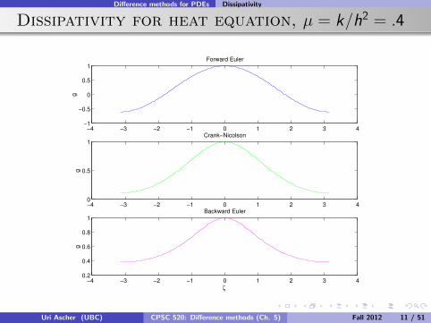
Observe that instability is caused by high wave numbers that do notnecessarily contribute to accuracy.
Hence, require damping of high wave number modes. The methodhas dissipativity of order 2r if
ρ(G (ζ)) ≤ eαk(1− δ|ζ|2r ), ∀|ζ| ≤ π.
Kreiss (60’s): This is sufficient for stability in many realistic situationsfor linear PDEs.
Generally, dissipativity is natural for parabolic PDEs but not forhyperbolic PDEs.
Uri Ascher (UBC) CPSC 520: Difference methods (Ch. 5) Fall 2012 10 / 51
Difference methods for PDEs Dissipativity
Dissipativity for heat equation, µ = k/h2 = .4
−4 −3 −2 −1 0 1 2 3 4−1
−0.5
0
0.5
1g
Forward Euler
−4 −3 −2 −1 0 1 2 3 40
0.5
1
g
Crank−Nicolson
−4 −3 −2 −1 0 1 2 3 40.2
0.4
0.6
0.8
1
ζ
g
Backward Euler
Uri Ascher (UBC) CPSC 520: Difference methods (Ch. 5) Fall 2012 11 / 51

Difference methods for PDEs Dissipativity
Dissipativity for heat equation, µ = k/h2 = 4
−4 −3 −2 −1 0 1 2 3 4−15
−10
−5
0
5g
Forward Euler
−4 −3 −2 −1 0 1 2 3 4−1
−0.5
0
0.5
1
g
Crank−Nicolson
−4 −3 −2 −1 0 1 2 3 40
0.5
1
ζ
g
Backward Euler
Uri Ascher (UBC) CPSC 520: Difference methods (Ch. 5) Fall 2012 12 / 51
Difference methods for PDEs Dissipativity
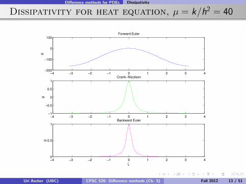
Dissipativity for heat equation, µ = k/h2 = 40
−4 −3 −2 −1 0 1 2 3 4−200
−100
0
100g
Forward Euler
−4 −3 −2 −1 0 1 2 3 4−1
−0.5
0
0.5
1
g
Crank−Nicolson
−4 −3 −2 −1 0 1 2 3 40
0.5
1
ζ
g
Backward Euler
Uri Ascher (UBC) CPSC 520: Difference methods (Ch. 5) Fall 2012 13 / 51

Difference methods for PDEs Hyperbolic systems
Outline
Freezing coefficients and dissipativity
Schemes for hyperbolic systems in 1D
Discontinuous solutions (Ch. 10)
Semi-Lagrangian methods
Nonlinear stability and energy method
Uri Ascher (UBC) CPSC 520: Difference methods (Ch. 5) Fall 2012 14 / 51

Difference methods for PDEs Hyperbolic systems
Outline: schemes for hyperbolic systems
Lax-Wendroff
Conservation laws
Leap-frog
Lax-Friedrichs
Upwind
Modified PDE
Box
Uri Ascher (UBC) CPSC 520: Difference methods (Ch. 5) Fall 2012 15 / 51

Difference methods for PDEs Hyperbolic systems
Lax-Wendroff scheme
For hyperbolic problems, “natural” discretizations do notautomatically possess dissipativity. Nonetheless, the Lax-Wendroffscheme is dissipative!
Derivation idea: Apply Taylor for u(t + k , x), viz.
u(t + k, x) = u + kut +k2
2utt + · · · ,
and replace t-derivatives by x-derivatives using the PDE.
For advection ut + aux = 0, we have ut = −aux andutt = (−aux)t = a2uxx . So, set µ = k/h and obtain
vn+1j =
(I − µ
2aD0 +
µ2
2a2D+D−
)vnj .
This gives accuracy order (2, 2).
Uri Ascher (UBC) CPSC 520: Difference methods (Ch. 5) Fall 2012 16 / 51

Difference methods for PDEs Hyperbolic systems
Lax-Wendroff scheme
vn+1j =
(I − µ
2aD0 +
µ2
2a2D+D−
)vnj .
Fourier analysis promises stability if CFL condition holds, i.e.,µ|a| ≤ 1. But what about dissipativity?
Calculating amplification factor, obtain
|g(ζ)| ≤ 1− δ|ζ|4
if the CFL condition holds.
Hence this scheme has dissipativity of order 4 and has guaranteedstability, under certain conditions, for variable coefficient problems.
Uri Ascher (UBC) CPSC 520: Difference methods (Ch. 5) Fall 2012 17 / 51

Difference methods for PDEs Hyperbolic systems
Conservation laws
Many nonlinear hyperbolic systems can be written as
ut + f(u)x = 0.
With Jacobian
A(u) =∂f
∂ucan write conservation law in non-conservation form
ut + A(u)ux = 0,
but the conservation form is often preferable.As usual, solution is constant along characteristics
dx
dt= a(u(t, x)).
So, the direction of the characteristic curves depends on the solutionthrough initial values u0(x), but the characteristic curves are straightlines.Uri Ascher (UBC) CPSC 520: Difference methods (Ch. 5) Fall 2012 18 / 51
Difference methods for PDEs Hyperbolic systems
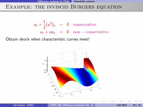
Example: the inviscid Burgers equation
ut +1
2(u2)x = 0 conservative
ut + uux = 0 non− conservative.
Obtain shock when characteristic curves meet!
Uri Ascher (UBC) CPSC 520: Difference methods (Ch. 5) Fall 2012 19 / 51

Difference methods for PDEs Hyperbolic systems
Example: Incompressible Navier-Stokes
Models incompressible fluid flow. In two space dimensions,(u, v)–velocity, p–pressure, ν–viscosity constant.
ut + uux + vuy + px = ν∆u,
vt + uvx + vvy + py = ν∆v ,
ux + vy = 0.
Use incompressibility to write material derivatives in conservationform: add u(ux + vy ) to first eqn, v(ux + vy ) to second, obtaining
ut + (u2)x + (vu)y + px = ν∆u,
vt + (uv)x + (v2)y + py = ν∆v ,
ux + vy = 0.
Uri Ascher (UBC) CPSC 520: Difference methods (Ch. 5) Fall 2012 20 / 51

Difference methods for PDEs Hyperbolic systems
Lax-Wendroff for conservation laws
Replacing 2nd time derivatives with spatial ones is trickier.
Want to avoid the Jacobian matrix A(u) if possible.
One popular variant:
vj =1
2(vnj + vnj+1)− 1
2µ(fnj+1 − fnj )
vn+1j = vnj − µ(f(vj)− f(vj−1))
Another popular variant:
vj = vnj − µ(fnj − fnj−1)
vn+1j =
1
2(vnj + vnj )− 1
2µ(f(vj+1)− f(vj)).
Uri Ascher (UBC) CPSC 520: Difference methods (Ch. 5) Fall 2012 21 / 51
Difference methods for PDEs Hyperbolic systems
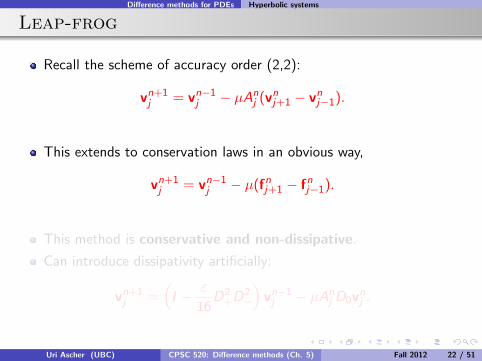
Leap-frog
Recall the scheme of accuracy order (2,2):
vn+1j = vn−1j − µAn
j (vnj+1 − vnj−1).
This extends to conservation laws in an obvious way,
vn+1j = vn−1j − µ(fnj+1 − fnj−1).
This method is conservative and non-dissipative.
Can introduce dissipativity artificially:
vn+1j =
(I − ε
16D2+D2−
)vn−1j − µAn
j D0vnj .
Uri Ascher (UBC) CPSC 520: Difference methods (Ch. 5) Fall 2012 22 / 51

Difference methods for PDEs Hyperbolic systems
Lax-Friedrichs
Recall the method for the advection equation
vn+1j =
1
2
(vnj+1 + vn
j−1)− k
2ha(vnj+1 − vn
j−1)
satisfies the strong stability bound ‖vn+1‖∞ ≤ ‖vn‖∞ provided CFLholds.
Write it for a linear hyperbolic system as
vn+1j = vnj +
1
2(vnj−1 − 2vnj + vnj+1)− µ
2Anj (vnj+1 − vnj−1),
highlighting the extra diffusion term in the modified PDE.
Method has accuracy order (1, 1) provided µ = k/h is fixed.
Uri Ascher (UBC) CPSC 520: Difference methods (Ch. 5) Fall 2012 23 / 51
Difference methods for PDEs Hyperbolic systems
Modified PDE
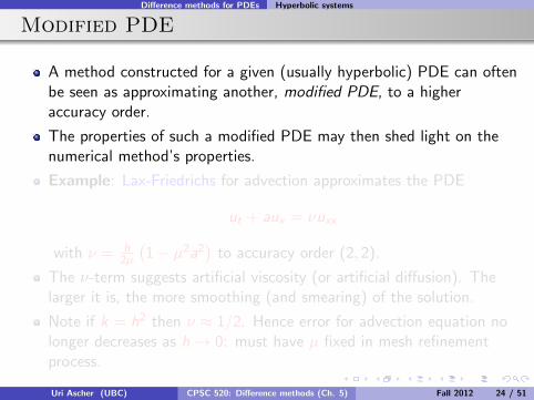
A method constructed for a given (usually hyperbolic) PDE can oftenbe seen as approximating another, modified PDE, to a higheraccuracy order.
The properties of such a modified PDE may then shed light on thenumerical method’s properties.
Example: Lax-Friedrichs for advection approximates the PDE
ut + aux = νuxx
with ν = h2µ
(1− µ2a2
)to accuracy order (2, 2).
The ν-term suggests artificial viscosity (or artificial diffusion). Thelarger it is, the more smoothing (and smearing) of the solution.
Note if k = h2 then ν ≈ 1/2. Hence error for advection equation nolonger decreases as h→ 0: must have µ fixed in mesh refinementprocess.
Uri Ascher (UBC) CPSC 520: Difference methods (Ch. 5) Fall 2012 24 / 51

Difference methods for PDEs Hyperbolic systems
Modified PDE
A method constructed for a given (usually hyperbolic) PDE can oftenbe seen as approximating another, modified PDE, to a higheraccuracy order.
The properties of such a modified PDE may then shed light on thenumerical method’s properties.
Example: Lax-Friedrichs for advection approximates the PDE
ut + aux = νuxx
with ν = h2µ
(1− µ2a2
)to accuracy order (2, 2).
The ν-term suggests artificial viscosity (or artificial diffusion). Thelarger it is, the more smoothing (and smearing) of the solution.
Note if k = h2 then ν ≈ 1/2. Hence error for advection equation nolonger decreases as h→ 0: must have µ fixed in mesh refinementprocess.
Uri Ascher (UBC) CPSC 520: Difference methods (Ch. 5) Fall 2012 24 / 51

Difference methods for PDEs Hyperbolic systems
Modified PDE for upwind and Lax-Wendroffschemes
Recall the upwind (one-sided) scheme for advection:
vn+1j = vn
j − µa
{(vnj+1 − vn
j
), a < 0(
vnj − vn
j−1), a > 0
.
This approximates the PDE ut + aux = νuxx withν = h
2µ
(µ|a| − µ2a2
)to accuracy order (2, 2).
So, both of these monotone 1st order schemes (i.e., upwind and L-F)have artificial viscosity, though upwind has less if µ|a| < 1.
The Lax-Wendroff scheme for advection has the modified PDE
ut + aux = −ah2
6
(1− µ2a2
)uxxx .
Note the 3rd rather than 2nd derivative in the added term!
Uri Ascher (UBC) CPSC 520: Difference methods (Ch. 5) Fall 2012 25 / 51
Difference methods for PDEs Hyperbolic systems
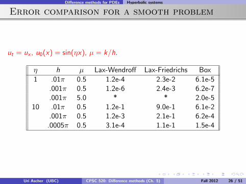
Error comparison for a smooth problem
ut = ux , u0(x) = sin(ηx), µ = k/h.
η h µ Lax-Wendroff Lax-Friedrichs Box
1 .01π 0.5 1.2e-4 2.3e-2 6.1e-5.001π 0.5 1.2e-6 2.4e-3 6.2e-7.001π 5.0 * * 2.0e-5
10 .01π 0.5 1.2e-1 9.0e-1 6.1e-2.001π 0.5 1.2e-3 2.1e-1 6.2e-4
.0005π 0.5 3.1e-4 1.1e-1 1.5e-4
Uri Ascher (UBC) CPSC 520: Difference methods (Ch. 5) Fall 2012 26 / 51

Difference methods for PDEs Hyperbolic systems
Error comparison for square wave µ = .5,h = .01π
−2 −1.5 −1 −0.5 0 0.5 1 1.5 2−0.5
0
0.5
1
1.5
u
Lax−Friedrichs scheme
−2 −1.5 −1 −0.5 0 0.5 1 1.5 2−0.5
0
0.5
1
1.5
uLax−Wendroff scheme
−2 −1.5 −1 −0.5 0 0.5 1 1.5 2−0.5
0
0.5
1
1.5
u
Leap−frog scheme
−2 −1.5 −1 −0.5 0 0.5 1 1.5 2−0.5
0
0.5
1
1.5
x
u
Leap−frog scheme with dissipation
Uri Ascher (UBC) CPSC 520: Difference methods (Ch. 5) Fall 2012 27 / 51

Difference methods for PDEs Hyperbolic systems
Error comparison for square wave µ = .5,h = .001π
−2 −1.5 −1 −0.5 0 0.5 1 1.5 2−0.5
0
0.5
1
1.5
u
Lax−Friedrichs scheme
−2 −1.5 −1 −0.5 0 0.5 1 1.5 2−0.5
0
0.5
1
1.5
uLax−Wendroff scheme
−2 −1.5 −1 −0.5 0 0.5 1 1.5 2−0.5
0
0.5
1
1.5
u
Leap−frog scheme
−2 −1.5 −1 −0.5 0 0.5 1 1.5 2−0.5
0
0.5
1
1.5
x
u
Leap−frog scheme with dissipation
Uri Ascher (UBC) CPSC 520: Difference methods (Ch. 5) Fall 2012 28 / 51

Difference methods for PDEs Hyperbolic systems
Box
Finite volume: Integrate conservation law ut + f(u)x = 0 over “box”
V = [xj , xj+1]× [tn, tn+1].
Obtainun+1j+1/2 − un
j+1/2 + fn+1/2j+1 − f
n+1/2j = 0
where quantities are line integrals.
Discretize by trapezoidal rule:
vn+1j+1 + vn+1
j − vnj+1 − vnj
+ µ(fn+1j+1 + fnj+1 − fn+1
j − fnj ) = 0.
The method is compact, conservative, implicit, unconditionallystable, and has accuracy order (2, 2).
Uri Ascher (UBC) CPSC 520: Difference methods (Ch. 5) Fall 2012 29 / 51

Difference methods for PDEs Semi-Lagrangian methods
Outline
Freezing coefficients and dissipativity
Schemes for hyperbolic systems in 1D
Discontinuous solutions (Ch. 10)
Semi-Lagrangian methods
Nonlinear stability and energy method
Uri Ascher (UBC) CPSC 520: Difference methods (Ch. 5) Fall 2012 30 / 51
Difference methods for PDEs Semi-Lagrangian methods
Outline
Freezing coefficients and dissipativity
Schemes for hyperbolic systems in 1D
Discontinuous solutions (Ch. 10)
Semi-Lagrangian methods
Nonlinear stability and energy method
Uri Ascher (UBC) CPSC 520: Difference methods (Ch. 5) Fall 2012 31 / 51

Difference methods for PDEs Semi-Lagrangian methods
Semi-Lagrangian (SL) method for advection
For the advection equation ut + aux = 0, extend the interpretation ofthe one-sided scheme as tracing the characteristic, by tracing thecharacteristic curve further back!
Imagine the one-sided scheme on a coarse grid with widths k = lkand h = lh for some l ≥ 1, but instead of interpolating between xjand xj+1 = xj + h, find ν such that xj+ν ≤ x∗ ≤ xj+ν+1 andinterpolate v n
j+ν and v nj+ν+1 linearly for v∗. Then set this value to be
v n+1j as before. The new time step is therefore l times larger, with
the same spatial mesh as before.
Explicit stability restriction is no longer binding because can increase larbitrarily for the (k , h) mesh, so, for a fixed h can take k arbitrarilylarge without stability concerns in this way!
Uri Ascher (UBC) CPSC 520: Difference methods (Ch. 5) Fall 2012 32 / 51

Difference methods for PDEs Semi-Lagrangian methods
Example: ut = ux with u0 a square wave
u0 square wave on [.25, .75], k = .9h, five times larger for SL, h = .01π
−3 −2 −1 0 1 2 3−0.5
0
0.5
1
1.5u
One−sided
−3 −2 −1 0 1 2 3−0.5
0
0.5
1
1.5
u
Leap−frog
−3 −2 −1 0 1 2 3−0.5
0
0.5
1
1.5
x
u
Semi−Lagrangian
Uri Ascher (UBC) CPSC 520: Difference methods (Ch. 5) Fall 2012 33 / 51

Difference methods for PDEs Semi-Lagrangian methods
Example: ut = ux with u0 a square wave
u0 square wave on [.25, .75], k = .9h, five times larger for SL, h = .001π
−3 −2 −1 0 1 2 3−0.5
0
0.5
1
1.5
uOne−sided
−3 −2 −1 0 1 2 3−0.5
0
0.5
1
1.5
u
Leap−frog
−3 −2 −1 0 1 2 3−0.5
0
0.5
1
1.5
x
u
Semi−Lagrangian
Uri Ascher (UBC) CPSC 520: Difference methods (Ch. 5) Fall 2012 34 / 51

Difference methods for PDEs Semi-Lagrangian methods
Second order semi-Lagrangian method:constant coefficients
The foot of the characteristic is at
x∗ = xj + ka = xj+ν + h∗, ν = fix((−a)k/h
), h∗ = wh.
The method we have seen is given by linear interpolation
vn+1j = v∗L = w ∗ vn
j+ν+1 + (1− w) ∗ vnj+ν ,
so it’s 1st order accurate.
To obtain 2nd order, can interpolate using also vj+ν+2, i.e., quadraticinterpolation:
vn+1j = v∗Q = v∗L − .5w(1− w)
(vnj+ν+2 − 2vn
j+ν+1 + vnj+ν
).
Numerical results for both smooth and square wave initial profiles:behaves essentially like Lax-Wendroff!
Uri Ascher (UBC) CPSC 520: Difference methods (Ch. 5) Fall 2012 35 / 51
Difference methods for PDEs Semi-Lagrangian methods
SL early assessment
For constant-coefficient advection the SL method looks “too good tobe true”!
Indeed, it makes heavy use of particular knowledge regarding a testequation, for which the exact solution is known.
Still, there are many fluid problems where non-constant advectionequations arise. Then, using a large time step, we are tradingaccuracy for stability.
Method is particularly useful in computer graphics and for weathersimulation applications.
Must extend the method to variable coefficient and nonlinearadvection problems.
Uri Ascher (UBC) CPSC 520: Difference methods (Ch. 5) Fall 2012 36 / 51

Difference methods for PDEs Semi-Lagrangian methods
SL for variable coefficient advection
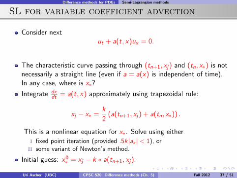
Consider nextut + a(t, x)ux = 0.
The characteristic curve passing through (tn+1, xj) and (tn, x∗) is notnecessarily a straight line (even if a = a(x) is independent of time).In any case, where is x∗?
Integrate dxdt = a(t, x) approximately using trapezoidal rule:
xj − x∗ =k
2(a(tn+1, xj) + a(tn, x∗)) .
This is a nonlinear equation for x∗. Solve using either
i fixed point iteration (provided .5k |ax | < 1), orii some variant of Newton’s method.
Initial guess: x0∗ = xj − k ∗ a(tn+1, xj).
Uri Ascher (UBC) CPSC 520: Difference methods (Ch. 5) Fall 2012 37 / 51
Difference methods for PDEs Semi-Lagrangian methods
SL for variable coefficient advection
Consider nextut + a(t, x)ux = 0.
The characteristic curve passing through (tn+1, xj) and (tn, x∗) is notnecessarily a straight line (even if a = a(x) is independent of time).In any case, where is x∗?
Integrate dxdt = a(t, x) approximately using trapezoidal rule:
xj − x∗ =k
2(a(tn+1, xj) + a(tn, x∗)) .
This is a nonlinear equation for x∗. Solve using either
i fixed point iteration (provided .5k |ax | < 1), orii some variant of Newton’s method.
Initial guess: x0∗ = xj − k ∗ a(tn+1, xj).
Uri Ascher (UBC) CPSC 520: Difference methods (Ch. 5) Fall 2012 37 / 51
Difference methods for PDEs Semi-Lagrangian methods
SL for variable coefficient advection cont.
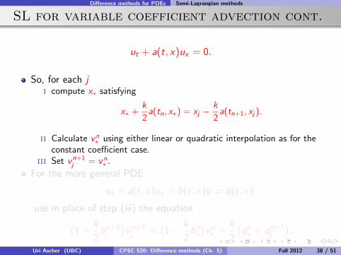
ut + a(t, x)ux = 0.
So, for each ji compute x∗ satisfying
x∗ +k
2a(tn, x∗) = xj −
k
2a(tn+1, xj).
ii Calculate vn∗ using either linear or quadratic interpolation as for the
constant coefficient case.iii Set vn+1
j = vn∗ .
For the more general PDE
ut + a(t, x)ux + b(t, x)u = q(t, x),
use in place of step (iii) the equation(1 +
k
2bn+1j
)vn+1j =
(1− k
2bn∗)vn∗ +
k
2
(qn∗ + qn+1
j
).
Uri Ascher (UBC) CPSC 520: Difference methods (Ch. 5) Fall 2012 38 / 51

Difference methods for PDEs Semi-Lagrangian methods
SL for variable coefficient advection cont.
ut + a(t, x)ux = 0.
So, for each ji compute x∗ satisfying
x∗ +k
2a(tn, x∗) = xj −
k
2a(tn+1, xj).
ii Calculate vn∗ using either linear or quadratic interpolation as for the
constant coefficient case.iii Set vn+1
j = vn∗ .
For the more general PDE
ut + a(t, x)ux + b(t, x)u = q(t, x),
use in place of step (iii) the equation(1 +
k
2bn+1j
)vn+1j =
(1− k
2bn∗)vn∗ +
k
2
(qn∗ + qn+1
j
).
Uri Ascher (UBC) CPSC 520: Difference methods (Ch. 5) Fall 2012 38 / 51
Difference methods for PDEs Semi-Lagrangian methods
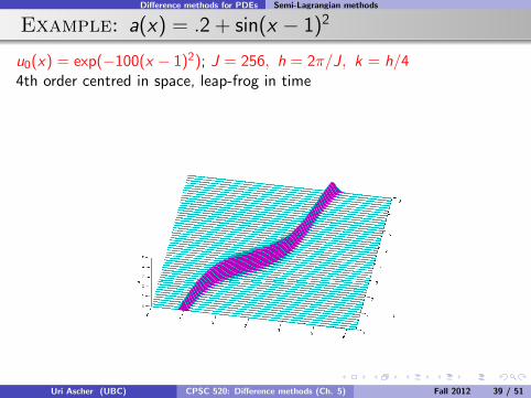
Example: a(x) = .2 + sin(x − 1)2
u0(x) = exp(−100(x − 1)2); J = 256, h = 2π/J, k = h/44th order centred in space, leap-frog in time
Uri Ascher (UBC) CPSC 520: Difference methods (Ch. 5) Fall 2012 39 / 51

Difference methods for PDEs Semi-Lagrangian methods
Example: a(x) = .2 + sin(x − 1)2
u0(x) = exp(−100(x − 1)2); J = 256, h = 2π/J, k = h/44th order centred in space, RK4 in time
Uri Ascher (UBC) CPSC 520: Difference methods (Ch. 5) Fall 2012 40 / 51
Difference methods for PDEs Semi-Lagrangian methods
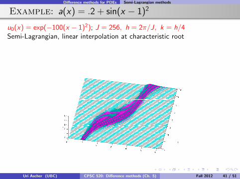
Example: a(x) = .2 + sin(x − 1)2
u0(x) = exp(−100(x − 1)2); J = 256, h = 2π/J, k = h/4Semi-Lagrangian, linear interpolation at characteristic root
Uri Ascher (UBC) CPSC 520: Difference methods (Ch. 5) Fall 2012 41 / 51

Difference methods for PDEs Semi-Lagrangian methods
Example: a(x) = .2 + sin(x − 1)2
u0(x) = exp(−100(x − 1)2); J = 256, h = 2π/J, k = h/4Semi-Lagrangian, quadratic interpolation at characteristic root
Uri Ascher (UBC) CPSC 520: Difference methods (Ch. 5) Fall 2012 42 / 51
Difference methods for PDEs Energy method
Outline
Freezing coefficients and dissipativity
Schemes for hyperbolic systems in 1D
Discontinuous solutions (Ch. 10)
Semi-Lagrangian methods
Nonlinear stability and energy method
Uri Ascher (UBC) CPSC 520: Difference methods (Ch. 5) Fall 2012 43 / 51

Difference methods for PDEs Energy method
Stability for nonlinear problems
We have seen in the KdV example that nonlinear stability can betricky: a Fourier stability analysis for the frozen coefficient problemgives (usually) necessary but not sufficient conditions: no guarantee.
Other examples exist: certainly for problems with discontinuoussolutions, but also splitting methods for the nonlinear Schrodingerequation, etc.
So instead try to bound
‖v(nk, ·)‖ ≤ ‖v(0, ·)‖
in the `2 norm, if a corresponding bound for the exact solution holds.
Uri Ascher (UBC) CPSC 520: Difference methods (Ch. 5) Fall 2012 44 / 51

Difference methods for PDEs Energy method
Energy method: PDE problem
Observe ∫ ∞−∞
2uutdx =∂
∂t
∫ ∞−∞
u2(t, x)dx .
So, for pure IVP (Cauchy) PDE
ut = f (t, x , ux , uxx , uxxx , ...),
if ∫ ∞−∞
uf (t, x , ux , uxx , uxxx , ...)dx ≤ 0
then ‖u(t)‖ ≤ ‖u(0)‖, ∀t ≥ 0, yielding L2-stability.
Uri Ascher (UBC) CPSC 520: Difference methods (Ch. 5) Fall 2012 45 / 51

Difference methods for PDEs Energy method
Energy method: PDE problem
Important tool: integration by parts. If f and g are periodic on [a, b]then
0 = f (b)g(b)− f (a)g(a) =
∫ b
a(fg)′dx =
∫ b
af ′gdx +
∫ b
afg ′dx .
Example: Cauchy problem for heat equation, or periodic BC for
ut = uxx .
Then∫
u · uxxdx = −∫
(ux(t, x))2 dx ≤ 0.So, ‖u(t)‖2 ≤ ‖u(0)‖2.
Uri Ascher (UBC) CPSC 520: Difference methods (Ch. 5) Fall 2012 46 / 51

Difference methods for PDEs Energy method
Energy method: discretized problem
For an infinite, uniform mesh, define
(v ,w) = h∞∑
j=−∞vj wj , ‖v‖2 = (v , v).
Identities:
∂
∂t(‖v‖2) = 2< (v , vt)
(v ,D0w) = −(D0v ,w), hence < (v ,D0v) = 0
(v ,D+w) = −(D−v ,w)
< (v ,Rv) = 0 ⇔ < (v ,Rw) = −< (Rw , v), ∀v ,w ∈ `2
Uri Ascher (UBC) CPSC 520: Difference methods (Ch. 5) Fall 2012 47 / 51

Difference methods for PDEs Energy method
Example: the Burgers equation
Obviously, for the pure initial value PDE
ut +1
2
(u2)x
= 0,
so long as the solution is smooth,
‖u(t)‖ = ‖u(0)‖ ∀t.
So does the KdV equation for all times.
Consider the discretizations D0
(v2)
for(u2)x
and 2vD0v for 2uux .
Obtain (v ,D0v2) = −(D0v , v2), which is different from2(v , vD0v) = 2(v2,D0v) = 2(D0v , v2).
Write Burgers as
ut +θ
2
(u2)x
+ (1− θ)uux = 0,
and discretize.Uri Ascher (UBC) CPSC 520: Difference methods (Ch. 5) Fall 2012 48 / 51

Difference methods for PDEs Energy method
Example: the Burgers equation cont.
Write Burgers as
ut +θ
2
(u2)x
+ (1− θ)uux = 0.
Discretize:
vt +1
2h
[θ
2D0v2 + (1− θ)vD0v
]= 0.
Multiply by v and sum up:
(v , vt) +1
2h
[θ
2(v ,D0v2) + (1− θ)(v , vD0v)
]= 0.
Choose θ = 2/3. Then θ/2 = 1− θ, so(‖v‖2
)t
= 0, hence
‖v(t)‖ = ‖v(0)‖ ∀t.
Obtain stability of semi-discretization so long as solution is smooth!
Uri Ascher (UBC) CPSC 520: Difference methods (Ch. 5) Fall 2012 49 / 51

Difference methods for PDEs Energy method
Example: the Burgers equation cont.
In the presence of shocks want to discretize the conservation formθ = 1.
But if solution is smooth, use θ = 2/3 for a stable semi-discretization.
Discretize in time: leap-frog may generate difficulties (recall KdVexample).
Using instead implicit midpoint, obtain method
vn+1j − vn
j +k
6h
(vn+1/2j+1 + v
n+1/2j + v
n+1/2j−1
)D0v
n+1/2j = 0.
Multiply by 2vn+1/2j and sum:
‖vn+1‖2−‖vn‖2+µ
3
(vn+1/2j , [v
n+1/2j+1 + v
n+1/2j + v
n+1/2j−1 ]D0v
n+1/2j
)= 0.
Hence ‖vn+1‖ = ‖vn‖ and the scheme is unconditionally stable.
Uri Ascher (UBC) CPSC 520: Difference methods (Ch. 5) Fall 2012 50 / 51

Difference methods for PDEs Energy method
RK for skew-symmetric semi-discretization
Consider a large constant-coefficient ODE system
vt = Lv,
where L is J × J skew-symmetric: LT = −L.
Obtain such L e.g. from symmetric (centred) semi-discretization of aconstant-coefficient hyperbolic PDE.
Note all eigenvalues of L are imaginary; and ‖v(t)‖ = ‖v(0)‖, ∀t.
Implicit midpoint in time stable for all k and conserves the invariant
‖vn‖ = ‖v0‖, ∀n.
If k ≤ 2√2
ρ(L) then the classical explicit RK4 satisfies
‖vn+1‖ ≤ ‖vn‖, ∀n.
See Example 5.12 (pp. 175–177) in the text.
Uri Ascher (UBC) CPSC 520: Difference methods (Ch. 5) Fall 2012 51 / 51