CS5263 Bioinformatics

Guest LecturePart II

Phylogenetics

Up to now we have focused onfinding similarities, now we startfocusing on differences(dissimilarities leadingto distance measures).Identifying sequences has beenThe goal so far. Now we are toarrange the sequences according totheir ancestry.

Phylogenetic trees are a graphicalrepresentation of the distancebetween sequences or species.Here we have the tree of the 3major groups of living organisms(excluding viruses).Until recently, most phylogenieswere based on rRNA sequences forprokaryotes and mitochondrialsequences for eukaryotes.

Terminology

• Phylogeny– The evolutionary relationships among organisms, based on a

common ancestor

• Phylogenetics– Area of research concerned with finding the genetic relationships

between species

(Greek: phylon = race and genetic = birth)

Terminology• Phylogenetic tree: Visual representation of evolutionary

distances between species

Introduction to terminology forphylogeny lecture

• Speciation• Gene Duplication• Homologous

– Orthologs– Paralogs

Allopatric speciation: populations are separated by a barrier.

After some time, even if the barrier is removed the two populations can nolonger form hybrids (now different species)

Sympatric speciation: the population shares the environment, mate selectioneffectively separates gene pools

Gene duplicationdiagram:

The three bands areduplicated.

Consider gene A is the ancestor species. Following duplication and modification, A1 and A2variants of gene A was fixated in the ancestor. The ancestor species diverged into species X and Y.The two variants A1 and A2 evolves independently in the two lineages into A1X - A2x, and A1Z -A2Z in species X and Z, respectively.Paralogous genes are derived from duplication, such as A1 and A2.Orthologous genes are derived from speciation, such as A1x - A1z, and A2x - A2z.

Genetic similarity among taxa should be estimated by comparing orthologoussequences. A phylogeny should be computed to determine which similar sequencesare orthologs.

Orthologues / Paralogues

Definitions

• Classic phylogenetic analysis usesmorphological features

• Anatomy, size, number of legs, beak shape…

• Modern phylogenetic analysis usesmolecular information

• Genetic material (DNA and protein sequences)

Molecular phylogenetic analysis

Phylogenetic reconstruction• Goal: given a set of species (genes), reconstruct the

tree which best explains their evolutionary history

Phylogenetic reconstruction

• “Nothing in evolution makes sense except in thelight of phylogeny.” -- Joe Felsenstein

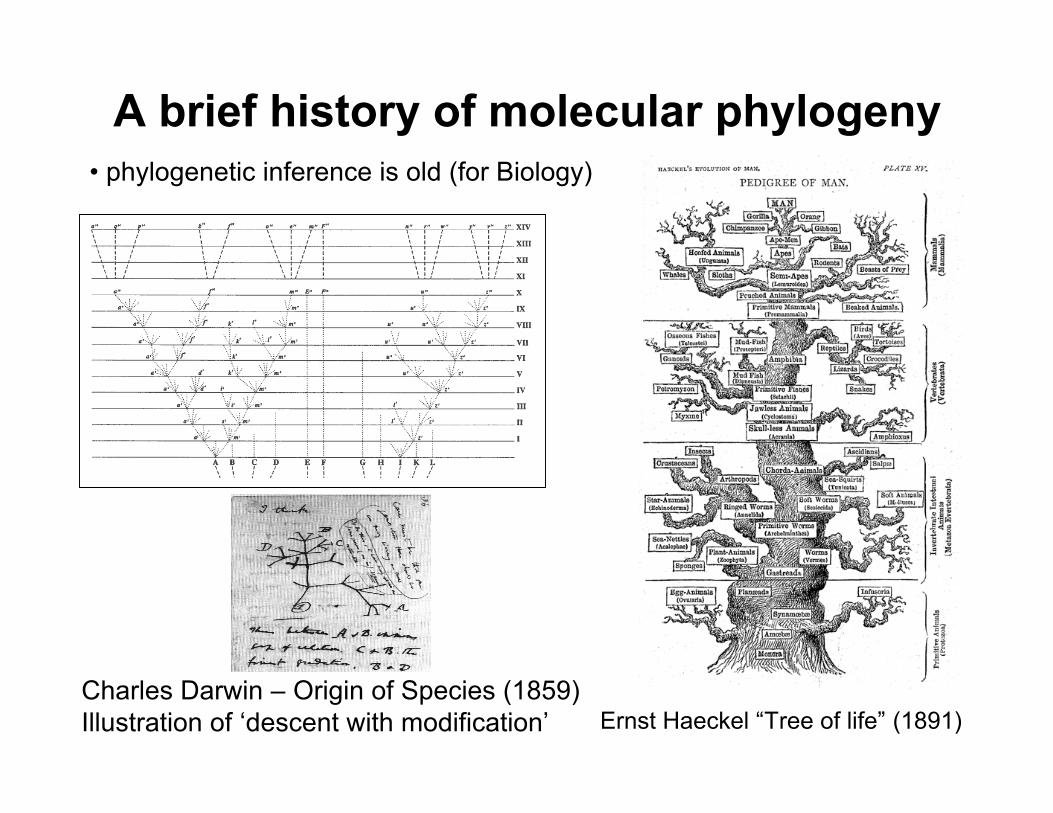
A brief history of molecular phylogeny• phylogenetic inference is old (for Biology)

Ernst Haeckel “Tree of life” (1891)Charles Darwin – Origin of Species (1859)Illustration of ‘descent with modification’

phylogeny – pattern and timing of evolutionary branchingevents (“evolutionary tree”)

Tracing evolutionary history

A B C D

common ancestorof A & B

common ancestorof C & D

common ancestorof A, B, C, D

branching happened in the past• common ancestors cannot be observed• must infer from data

internal node - commonancestor (CA)external node - operationaltaxonomic unit (OTU)order of branches define therelationships (topology)branch length defines thenumber of changes

Unrooted versus rooted phylogenies

What are phylogenies good for?(1) classification

• Systematics: a scientific field devoted toclassification of organisms– Phenetics: a classification scheme based on

grouping populations according to similarities– Cladistics: a classification scheme based on

evolutionary relationships (phylogenies)

Monophyletic vs paraphyletic

• Monophyletic group: includingall descendents of a commonancestor

• Paraphyletic group: a set ofspecies that includes acommon ancestor and some,but not all, of its descendants.

Paraphyletic groups

What are phylogenies good for?(2) detecting coevolution

• Aphid-bacteria• Mutualistic• cospeciation

What are phylogenies good for?(3) origin of pathogens

• Black plague• Pathogen: Yersinia

pestis• 36 strains

What are phylogenies good for?(4) Tree of life

Animal Kingdom

Rrooting the tree:

To root a tree mentally,imagine that the tree ismade of string. Grab thestring at the root andtug on it until the ends ofthe string (the taxa) fallopposite the root: A

BC

Root D

A B C D

RootNote that in this rooted tree, taxon A isno more closely related to taxon B thanit is to C or D.

Rooted tree

Unrooted tree

n

∏ (2i-5) • (2n-3) i=3

Number of OTUs (tips) vs.number of possible trees

# rooted trees

2 1 1 3 1 3 4 3 15 5 15 105 6 105 954 7 954 10,395 8 10,395 135,135 9 135,135 2,027,02510 2,027,025 34,459,425

true tree - true evolutionary history is one of many possibilities.difficult to infer true tree when # OTUs is large

inferred tree - obtained using data and reconstruction method.not necessarily the same as the true tree - a hypothesis

n

∏ (2i-5) i=3

# OTUs (n)# unrooted trees

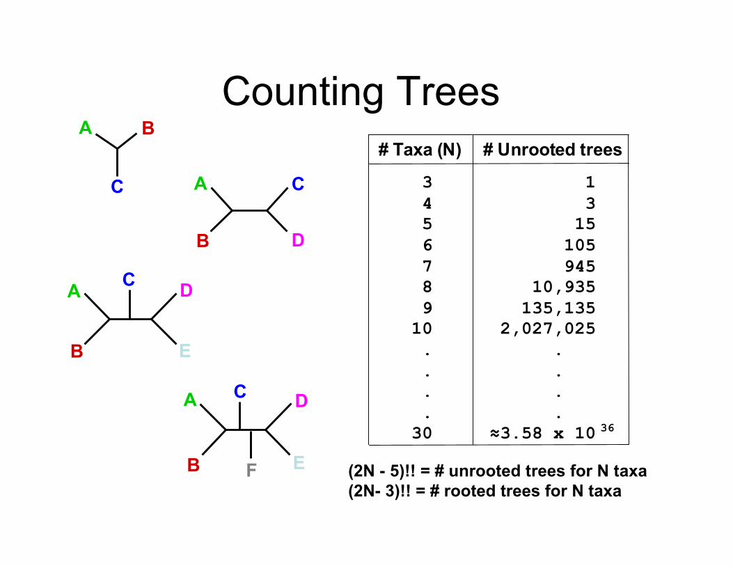
Counting Trees# Taxa (N)

3

4

5

6

7

8

9

10

.

.

.

.

30

# Unrooted trees

1

3

15

105

945

10,935

135,135

2,027,025

.

.

.

.

!3.58 x 10 36

(2N - 5)!! = # unrooted trees for N taxa(2N- 3)!! = # rooted trees for N taxa

CA

B D

A B

C

A D

B E

C

A D

B E

C

F

Reconstruct phylogenetic trees

Methods of phylogenetic reconstruction• Distance based

– pairwise evolutionary distances computed for all taxa– tree constructed using algorithm based on relationships

between distances• Maximum parsimony

– nucleotides or amino acids are considered as character states– best phylogeny is chosen as the one that minimizes the number

of changes between character states• Maximum likelihood

– statistical method of phylogeny reconstruction– explicit model for how data set generated - nucleotide or amino

acid substitution– find topology that maximizes the probability of the data given

the model and the parameter values (estimated from data)

2. Determine the evolutionarydistances and build distance matrix

• For molecular data, evolutionary distancescan be the observed number of nucleotidedifferences between the pairs of species.

• Distance matrix: simply a table showingthe evolutionary distances between allpairs of sequences in the dataset

2. Determine the evolutionary distances and builddistance matrix - A simple example using DNA

sequences

AGGCCATGAATTAAGAATAA2. AGCCCATGGATAAAGAGTAA3. AGGACATGAATTAAGAATAA4. AAGCCAAGAATTACGAATAA

Distance Matrix

In this example the evolutionarydistance is expressed as thenumber of nucleotide differencesfor each sequence pair. Forexample, sequences 1 and 2 are20 nucleotides in length and havefour differences, corresponding toan evolutionary difference of 4/20= 0.2.-4

0.2-3

0.40.25-2

0.150.050.2-1

4321

3. Phylogenetic Tree Constructionexample (UPGMA algorithm)

1. Pick smallest entry Dij

2. Join the two intersecting species and assign branch lengthsDij/2 to each of the nodes

-Seal

0.44-Weasel

0.440.42-Raccoon

0.290.340.26-Bear

SealWeaselRaccoonBearDij Bear Raccoon

0.13 0.13

UPMGA (Michener & Sokal 1957)

3. Phylogenetic Tree Constructionexample (UPGMA algorithm)

-Seal

0.44-Weasel

0.440.42-Raccoon

0.290.340.26-Bear

SealWeaselRaccoonBearDij

3. Compute new distances to the other species usingarithmetic means

365.02

44.029.0

2

38.02

42.034.0

2

)(

)(

=+

=+

=

=+

=+

=

SRSB

BRS

WRWB

BRW

DDD

DDD

Bear Raccoon

0.13 0.13

3. Phylogenetic Tree Constructionexample (UPGMA algorithm)

-Seal

0.44-Weasel

0.3650.38-BR

SealWeaselBRDij

1. Pick smallest entry Dij

2. Join the two intersecting species and assign branch lengths Dij/2 to each of the nodes

Bear Raccoon Seal

0.13 0.1825 0.1825

3. Phylogenetic Tree Constructionexample (UPGMA algorithm)

-Seal

0.44-Weasel

0.3650.38-BR

SealWeaselBRDij

3. Compute new distances to the other species usingarithmetic means

4.03

44.042.034.0

3)( =

++=

++= WSWRWB

BRSW

DDDD

Bear Raccoon Seal

0.13 0.1825 0.1825

3. Phylogenetic Tree Constructionexample (UPGMA algorithm)

-Weasel

0.4-BRS

WeaselBRSDij

1. Pick smallest entry Dij.

2. Join the two intersecting species and assign branch lengthsDij/2 to each of the nodes.

3. Done!

Bear Raccoon Seal Weasel

0.13 0.1825

0.2 0.2

UPGMA clustering can be done using protein sequences

Calculation of a phylogeny from molecularcomparisons.

Cytochrome c comparisons (from Fitchand Margoliash, Science Vol. 155, 20 Jan.1967). The selected comparisons havebeen arranged randomly (no particularorder), as this makes no difference in theapplication of UPGMA (unweighted pair-group method using arithmetic averages)clustering.

The numbers in the cells show differencesbetween the cytochrome c molecules ofvarious species: for example, there is only1 difference in the amino acid sequencesbetween man and monkey, but there are19 differences between man and turtle.

The UPGMA method

• The UPGMA method is applied to the cytochrome c data sample. Ateach cycle of the method, the smallest entry is located, and theentries intersecting at that cell are "joined." The height of the branchfor this junction is one-half the value of the smallest entry. Thus,since the smallest entry at the beginning is 1 (between B=man andF=monkey), B and F are joined with branch heights of 0.5 (=1.0/2).Then, the comparison matrix is reduced by combining cells. Thesecombinations are indicated with colors in the next slide. Forexample, the comparisons of A to B (19.0) and A to F (18.0) areconsolidated as 18.5 = (19.0+18.0)/2 (red cells), while thecomparisons of E to B (36.0) and E to F (35.0.0) are consolidatedas 35.5 = (36.0+35.0)/2 (blue cells).

• The process is repeated on the reduced comparison matrix,resulting in a smaller matrix with each cycle. When the matrix iscompletely reduced, the calculation is finished.

What makes such calculations of phylogenies interesting is the fact that the results so often agreewith evolutionary trees developed from other methods (anatomy, fossils, or other proteins orgenes). Indeed, molecular comparisons provide ample "repeat experiments" of the hypothesis ofevolution.

The final phylogeny calculated from tables. It is in perfect accord with the fossil record,showing fish ancestral to reptiles, reptiles ancestral to mammals, birds splitting fromreptiles after the reptile/mammal split, and so forth. The lengths of branches indicatetime since last common ancestry; for example, moths and tuna (18.2 branch length)separated long before turtles and chickens (4.0 branch length).

Weakness of UPGMA• UPGMA assumes a constant molecular clock

(i.e. accumulate mutations at the same rate)– All leaves in the same level

• Only constructs rooted trees

23

41 1 4 32

Correct tree UPGMA

Example: morphology-based input

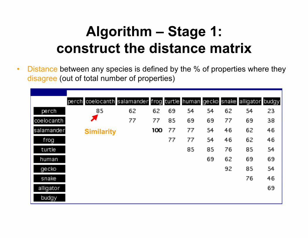
Algorithm – Stage 1:construct the distance matrix

• Distance between any species is defined by the % of properties where theydisagree (out of total number of properties)

Similarity

Algorithm – Stage 2:cluster close neighbors

• Iteration #1: identify the two closest taxa from the distancematrix

• In our case, one pair has zero distance: salamander & frog• We join them together, and update the distance matrix• Updated matrix has only 9 species (8 “old”, 1 new).

Algorithm – Stage 2:cluster close neighbors

• Iteration #2: join the gecko andsnake.

• Add the new pair to the forest,equally distributing their distance (8)

• Update the distance matrix• One must calculate the similarity of

each as-yet ungrouped taxa to thetwo groups already formed above

• Also calculate the similarity of thetwo groups to each other

Tie problem

Tie problem

• If you break ties “systematically”, according to the order ofappearance in the matrix, you will get the tree1; if you break tiesrandomly, you make get the tree 2

3 - choose pair of OTUs that minimizes total branch lengths in the tree4 - this pair collapsed as single OTU and distance matrix recalculated5 - next pair of OTUs that gives smallest branch length is chosen6 - iterate until complete

1 - start with star tree - no topologyS = total branch length of tree

2 - separate pair of OTUs from all othersS12 = total branch length of tree

uses ‘star decomposition’ – identification of neighbors that sequentially minimize the total length of the tree

Distance method(2) Neighbor-joining (NJ) method

The “1-star” Sum of the BranchLengths

)1/(

1

1

1

!=

!== ""

<=

NT

DN

LSN

ji

ij

N

i

ixo

• D and L as the distance between OTUsand the branch length between nodes

• Each branch is counted N-1 times whenall distances are added

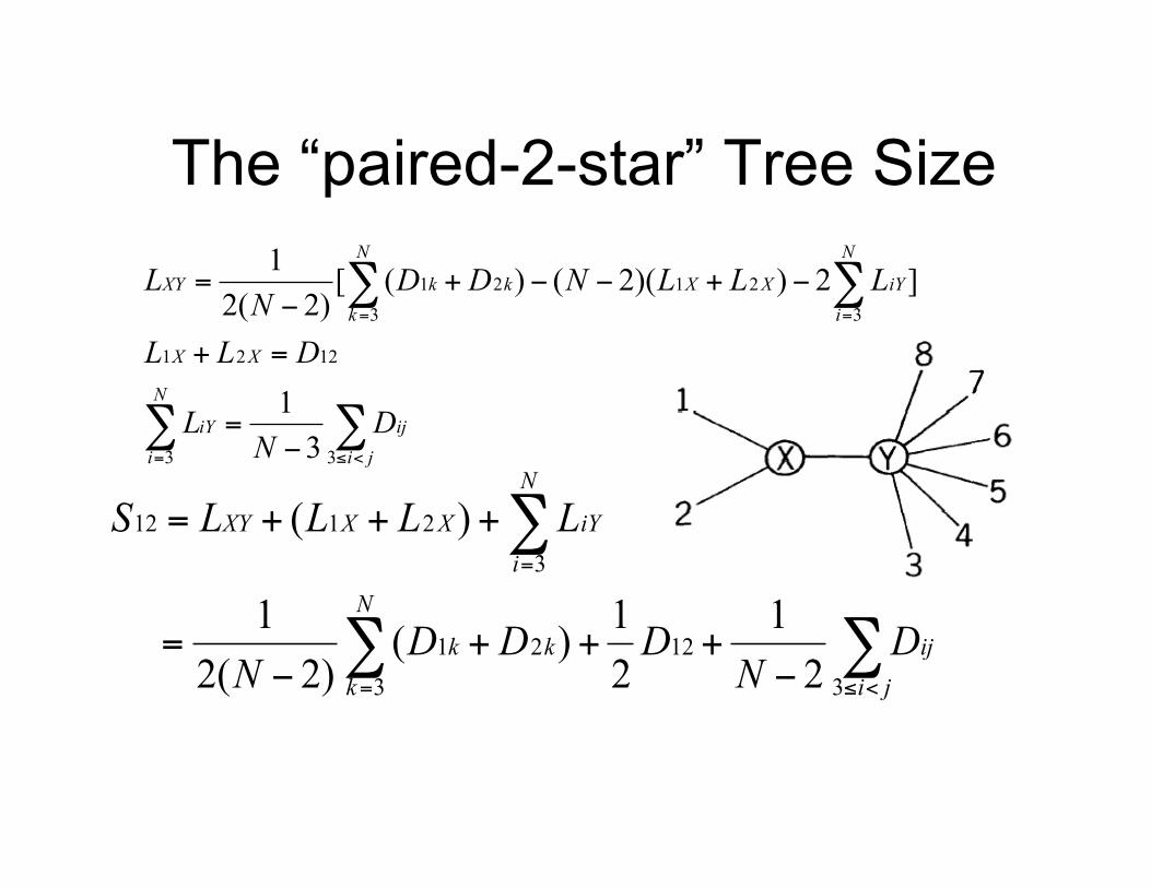
The “paired-2-star” Tree Size

!!

!

<"=

=

#+++

#=

+++=

ji

ij

N

k

kk

N

i

iYXXXY

DN

DDDN

LLLLS

3

12

3

21

3

2112

2

1

2

1)(

)2(2

1

)(

!!

!!

<"=

==

#=

=+

#+##+#

=

ji

ijiY

N

i

XX

N

i

iYXX

N

k

kkXY

DN

L

DLL

LLLNDDN

L

33

1221

3

21

3

21

3

1

]2))(2()([)2(2

1

Neighbor-joining example

Neighbor-Joining: Complexity

• The method performs a search using timeO(n2) and using time O(n2) to updatedistance matrix.

• Giving a total time complexity of O(n3),anda space complexity of O(n2).

Neighbor-joining method …• Extremely fast and efficient method, widely used• Tends to perform fairly well in simulation studies• May produce tie trees from data set but this appears to

be rare• Algorithm is ‘greedy’ and so can get stuck in local optima• Main criticism is that it produces only one tree and does

not give any idea of how many other trees are equallywell or almost as supported by the data

Maximum Parsimony (MP)What is parsimony?• A criterion for selecting among alternative

patterns based on minimizing the totalamount of evolutionary change

• Ancestral characters are inferred for eachsite and the total number of changesbetween nodes for a given topology aredetermined

• Best topology is the one that requires thefewest number of residue changesbetween nodes across all sites

A

A

C

C

Counting substitutions on a tree• For an alignment site and a topology, ancestral residues are inferred sothat the minimum number of residue changes between nodes is required

A

A

C

C

A C

A

A

G

T

A

A

G

T A

A

G

T A

A

G

T

A A

A

A

G

TUnambiguous (1) Ambiguous (2)

Sites 3 6 8 Tree I 4 steps best tree

Tree II 5 steps

Tree III 6 steps

T C A G A T C T A GT T A G A A C T A GT T C G A T C G A GT T C T A A G G A C

OTU 1 2 3 4 5 6 7 8 9 10 Site 1 2 3 4

Lecture #7 Page 5

Choosing the shortest tree with parsimony

1A 3C

2A 4C

1T 3T

2A 4A

1T 3G

2T 4G

1A 2A

3C 4C

1T 2A

3T 4A

1T 2T

3G 4G

1A 2A

4C 3C

1T 2A

4A 3T

1T 2T

3G 4G

A C

AA

C C

AA

AT

T T

T G

T T

G G

Advantages and disadvantages of parsimony

• Advantages:– based on a logically coherent and biologically plausible model of

evolution– free from assumptions used in distance estimations– better than distance methods when extent of sequence divergence is low

(10%), rate of substitution is constant, number of residues is large– very useful for certain types of molecular data e.g. indels

• Disadvantages:– gives incorrect topologies when backward substitutions are present

(common with nucleotides) and when the number of sites is fairly small– gives incorrect topologies when rate of substitution varies substantially

across lineages– long branch attraction – long branches (and short branches) tend to

group together on reconstructed tree– difficult to treat the results in a statistical framework

Maximum Likelihood• Statistical (probabilistic) method for inferring

phylogenies– substitution model is chosen for sequence data

(alignment)– likelihood of observing the sequence data given the

substitution model is obtained for each topologyevaluated (parameter fitting on branch lengths)

• Probability of each tree is product of mutation rates in eachbranch

• Likelihoods given by each column multiplied to give thelikelihood of the tree

– topology that gives the highest likelihood is chosen asthe best tree

Maximum Likelihood

• Extremely slow method so heuristicmethods almost always have to beemployed to search for best tree

• Method very dependent on model ofsubstitution used

• Method estimates branch lengths nottopology, so may give wrong topology

Assessing significance of Tree

• need some way to assess the support for thetopologies (evolutionary relationships) ofreconstructed phylogenies

1

2

3

4

?1

2

3

4

or

• bootstrapping: re-sample alignment andconstruct trees from re-sampled data

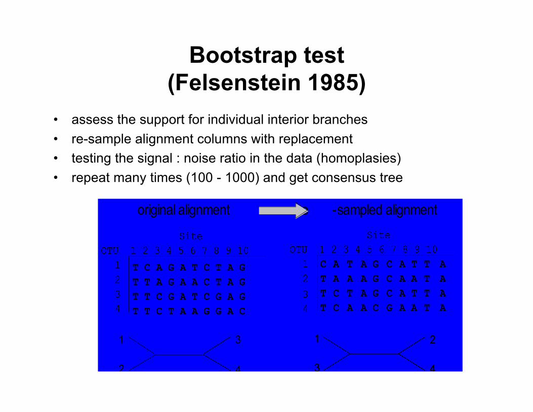
Bootstrap test(Felsenstein 1985)

• assess the support for individual interior branches• re-sample alignment columns with replacement• testing the signal : noise ratio in the data (homoplasies)• repeat many times (100 - 1000) and get consensus tree

T C A G A T C T A G

T T A G A A C T A G

T T C G A T C G A G

T T C T A A G G A C

Site

OTU 1 2 3 4 5 6 7 8 9 10

1

2

3

4

Site

OTU 1 2 3 4 5 6 7 8 9 10

1

2

3

4

C

T

T

T

A

A

C

C

T

A

T

A

A

A

A

A

Site

OTU 1 2 3 4 5 6 7 8 9 10

1

2

3

4

Site

OTU 1 2 3 4 5 6 7 8 9 10

1

2

3

4

G

G

G

C

C

C

C

G

A

A

A

A

T

A

T

A

T

T

T

T

A

A

A

A

original alignment re -sampled alignment

1

2

3

4

1

3

2

4

1

3

2

4

Interpreting bootstrap results

• 71 = the percentage of trees built from re-sampled alignments thatincluded the interior branch in question

• bootstrap values are said to “support”– that interior branch– the interior nodes adjacent (terminal) to the branch

1

2

3

4

71

1

2

3

4

71

• Rule of the thumb: >70% considered good evidence forproper placement of branches

• <50%, uncertain (unresolved) branching pattern(polytomy)

Comparison of Methods

Good for very small datasets and for testing treesbuilt using other methods

Best option whentractable (<30 taxa)

Good for generatingtentative tree, or choosingamong multiple trees, orworking on large-scaledata sets

Highly dependent onassumed evolution model

Assumptions fail whenevolution is rapid (Longbranch attraction)

Easily trapped in localoptima

Very slowSlowVery fast

Maximizes tree likelihoodgiven specific parametervalues

Minimizes totaldistance

Minimizes distancebetween nearestneighbors

Uses all dataUses only sharedderived characters

Uses only pairwisedistances

Maximum likelihoodMaximum parsimonyNeighbor-joining

Which Method to Choose?

• depends upon the sequences that arebeing compared– strong sequence similarity:

• maximum parsimony– clearly recognizable sequence similarity

• distance methods– All others:

• maximum likelihood

• Best to choose at least two approaches• Compare the results – if they are similar,

you can have more confidence

Which programs to use?

• Distance method:– MEGA

• Maximum Parsimony method– PAUP– MacClade

• Maximum Likelihood method– PHYLIP– PAML

Phylogenetics and forensic evidence

• Victim & patient strains more closely related to each other than controls (monophyletic)• Victims’ HIV sequences were a subset of the doctor’s patient’s sequences• Doctor guilty of attempted murder

• Louisiana doctor accused of injecting victim with HIV• Baylor grad student compares sequences of victim’s HIV & Doctor’s patient HIV & local control strains

Phylogenetics and forensic evidence ...

Phylogenetics and forensic evidence

Bayesian and GA software

• BEAST (Bayesian Evolutionary Analysis SamplingTrees): bayesian, MCMC

• MrBayes: bayesian, MCMC and MCMCMC• Phycas: bayesian, for DNA seqs, python• GARLI (Genetic Algorithm for Rapid Likelihood

Inference): uses a stochastic genetic algorithm-likeapproach, Computational analogue of evolution bynatural selection, not actually genetic algorithm

Software to evaluate trees

• Readseq is a program that edits sequences into18 different formats

• AWTY (are we there yet?) is used to calculatewhether MCMC has run long enough

• Tracer is similarly used to analyze MCMC basedprogram runs

• FigTree is used to edit trees for publication

• And so much more

Probabilistic Methods• The phylogenetic tree represents a generative

probabilistic model (like HMMs) for the observedsequences.

• Background probabilities: q(a)• Mutation probabilities: P(a|b, t)• Models for evolutionary mutations

– Jukes Cantor– Kimura 2-parameter model

• Such models are used to derive the probabilities

Jukes Cantor model

• A model for mutation rates

• Mutation occurs at aconstant rate• Each nucleotide isequally likely to mutateinto any other nucleotidewith rate a.

Kimura 2-parameter model

• Allows a different rate for transitions andtransversions.

Optimal Tree Search• Perform search over possible topologies

T1 T3

T4

T2

Tn

Parametricoptimization

(EM)

Parameter space

Local Maxima

Computational Problem• Such procedures are computationally expensive!• Computation of optimal parameters, per candidate,

requires non-trivial optimization step.• Spend non-negligible computation on a candidate, even

if it is a low scoring one.• In practice, such learning procedures can only consider

small sets of candidate structures

Current status of phylogeneticanalysis

• Bayesian approaches widely implemented• Maximum likelihood remains gold-standard• Novel genetic algorithms also currently

implemented, but not yet widely tested• Large datasets still very computationally

expensive• Very few reiterative methods where phylogeny

directs alignments and vice-versa• Still difficult for biologists to evaluate results of

different algorithms

Useful links• IUPAC codeshttp://www.bioinformatics.org/sms/iupac.html

• Molecular Evolution Course websitehttp://www.molecularevolution.org/

• Tree of Life web projecthttp://tolweb.org/tree/

http://bioinfoserver.rsbs.anu.edu.au/programs/index.php

• Introduction to evolution

http://evolution.berkeley.edu/

ReferencesUPGMA protein example:http://www.nmsr.org/upgma.htm

• Joe Felsenstein, Phylogeny methods,http://evolution.gs.washington.edu/gs541/2005/lecture26.pdf