1

CS590D: Data MiningProf. Chris Clifton

March 3, 2005Midterm Review

Midterm Thursday, March 10, 19:00-20:30, CS G066. Open book/notes.

2

Course Outlinehttp://www.cs.purdue.edu/~clifton/cs590d

1. Introduction: What is data mining?– What makes it a new and unique

discipline?– Relationship between Data

Warehousing, On-line Analytical Processing, and Data Mining

– Data mining tasks - Clustering, Classification, Rule learning, etc.

2. Data mining process – Task identification– Data preparation/cleansing– Introduction to WEKA

3. Association Rule mining– Problem Description– Algorithms

4. Classification / Prediction– Bayesian– Tree-based approaches– Regression– Neural Networks

5. Clustering– Distance-based approaches– Density-based approaches– Neural-Networks, etc.

6. Concept Description– Attribute-Oriented Induction– Data Cubes

7. More on process - CRISP-DMMidterm

Part II: Current Research9. Sequence Mining10. Time Series11. Text Mining12. Multi-Relational Data Mining13. Suggested topics, project

presentations, etc.

Text: Jiawei Han and Micheline Kamber, Data Mining: Concepts and Techniques. Morgan Kaufmann Publishers, August 2000.

2

CS590D Review 3

Data Mining: Classification Schemes

• General functionality– Descriptive data mining – Predictive data mining

• Different views, different classifications– Kinds of data to be mined– Kinds of knowledge to be discovered– Kinds of techniques utilized– Kinds of applications adapted

CS590D Review 4

adapted from:U. Fayyad, et al. (1995), “From Knowledge Discovery to Data Mining: An Overview,” Advances in Knowledge Discovery and Data Mining, U. Fayyad et al. (Eds.), AAAI/MIT Press

DataTargetData

Selection

KnowledgeKnowledge

PreprocessedData

Patterns

Data Mining

Interpretation/Evaluation

Knowledge Discovery in Databases: Process

Preprocessing

3

CS590D Review 6

Data Preprocessing

• Data in the real world is dirty– incomplete: lacking attribute values, lacking certain

attributes of interest, or containing only aggregate data

• e.g., occupation=“”

– noisy: containing errors or outliers• e.g., Salary=“-10”

– inconsistent: containing discrepancies in codes or names

• e.g., Age=“42” Birthday=“03/07/1997”• e.g., Was rating “1,2,3”, now rating “A, B, C”• e.g., discrepancy between duplicate records

CS590D Review 9

Major Tasks in Data Preprocessing

• Data cleaning– Fill in missing values, smooth noisy data, identify or remove

outliers, and resolve inconsistencies• Data integration

– Integration of multiple databases, data cubes, or files• Data transformation

– Normalization and aggregation• Data reduction

– Obtains reduced representation in volume but produces the same or similar analytical results

• Data discretization– Part of data reduction but with particular importance, especially

for numerical data

4

CS590D Review 10

How to Handle Missing Data?

• Ignore the tuple: usually done when class label is missing (assuming the tasks in classification—not effective when the percentage of missing values per attribute varies considerably.

• Fill in the missing value manually: tedious + infeasible?• Fill in it automatically with

– a global constant : e.g., “unknown”, a new class?! – the attribute mean– the attribute mean for all samples belonging to the same class:

smarter– the most probable value: inference-based such as Bayesian

formula or decision tree

CS590D Review 11

How to Handle Noisy Data?

• Binning method:– first sort data and partition into (equi-depth) bins– then one can smooth by bin means, smooth by bin

median, smooth by bin boundaries, etc.• Clustering

– detect and remove outliers• Combined computer and human inspection

– detect suspicious values and check by human (e.g., deal with possible outliers)

• Regression– smooth by fitting the data into regression functions

5

CS590D Review 12

Data Transformation

• Smoothing: remove noise from data• Aggregation: summarization, data cube

construction• Generalization: concept hierarchy climbing• Normalization: scaled to fall within a small,

specified range– min-max normalization– z-score normalization– normalization by decimal scaling

• Attribute/feature construction– New attributes constructed from the given ones

CS590D Review 13

Data Transformation: Normalization

• min-max normalization

• z-score normalization

• normalization by decimal scaling

AAA

AA

A

minnewminnewmaxnewminmax

minvv _)__(' +−

−−=

A

A

devstand_

meanvv

−='

j

vv

10'= Where j is the smallest integer such that Max(| |)<1'v

6

CS590D Review 14

Data Reduction Strategies

• A data warehouse may store terabytes of data– Complex data analysis/mining may take a very long time to run

on the complete data set• Data reduction

– Obtain a reduced representation of the data set that is much smaller in volume but yet produce the same (or almost the same) analytical results

• Data reduction strategies– Data cube aggregation– Dimensionality reduction — remove unimportant attributes– Data Compression– Numerosity reduction — fit data into models– Discretization and concept hierarchy generation

CS590D Review 15

Principal Component Analysis

• Given N data vectors from k-dimensions, find c ≤k orthogonal vectors that can be best used to represent data – The original data set is reduced to one consisting of N

data vectors on c principal components (reduced dimensions)

• Each data vector is a linear combination of the c principal component vectors

• Works for numeric data only• Used when the number of dimensions is large

7

CS590D Review 16

Numerosity Reduction

• Parametric methods– Assume the data fits some model, estimate

model parameters, store only the parameters, and discard the data (except possible outliers)

– Log-linear models: obtain value at a point in m-D space as the product on appropriate marginal subspaces

• Non-parametric methods– Do not assume models– Major families: histograms, clustering,

sampling

CS590D Review 17

Regress Analysis and Log-Linear Models

• Linear regression: Y = α + β X– Two parameters , α and β specify the line and are to

be estimated by using the data at hand.– using the least squares criterion to the known values

of Y1, Y2, …, X1, X2, ….• Multiple regression: Y = b0 + b1 X1 + b2 X2.

– Many nonlinear functions can be transformed into the above.

• Log-linear models:– The multi-way table of joint probabilities is

approximated by a product of lower-order tables.– Probability: p(a, b, c, d) = αab βacχad δbcd

8

CS590D Review 18

Sampling

• Allow a mining algorithm to run in complexity that is potentially sub-linear to the size of the data

• Choose a representative subset of the data– Simple random sampling may have very poor performance in the

presence of skew

• Develop adaptive sampling methods– Stratified sampling:

• Approximate the percentage of each class (or subpopulation of interest) in the overall database

• Used in conjunction with skewed data

• Sampling may not reduce database I/Os (page at a time).

CS590D Review 19

Discretization

• Three types of attributes:– Nominal — values from an unordered set– Ordinal — values from an ordered set– Continuous — real numbers

• Discretization: – divide the range of a continuous attribute into

intervals– Some classification algorithms only accept categorical

attributes.– Reduce data size by discretization– Prepare for further analysis

9

CS590D Review 20

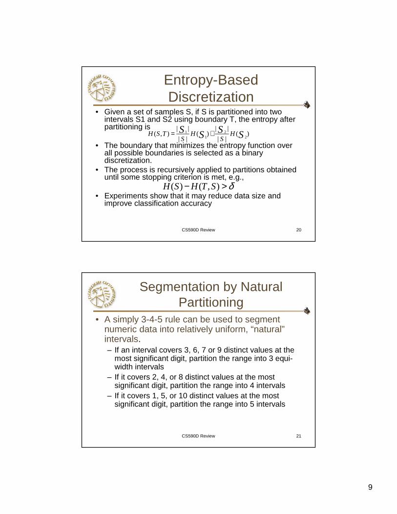
Entropy-Based Discretization

• Given a set of samples S, if S is partitioned into two intervals S1 and S2 using boundary T, the entropy after partitioning is

• The boundary that minimizes the entropy function over all possible boundaries is selected as a binary discretization.

• The process is recursively applied to partitions obtained until some stopping criterion is met, e.g.,

• Experiments show that it may reduce data size and improve classification accuracy

1 21 2

| | | |( , ) ( ) ( )

| | | |H S T H H

S SS SS S= +

( ) ( , )H S H T S δ− >

CS590D Review 21

Segmentation by Natural Partitioning

• A simply 3-4-5 rule can be used to segment numeric data into relatively uniform, “natural”intervals.– If an interval covers 3, 6, 7 or 9 distinct values at the

most significant digit, partition the range into 3 equi-width intervals

– If it covers 2, 4, or 8 distinct values at the most significant digit, partition the range into 4 intervals

– If it covers 1, 5, or 10 distinct values at the most significant digit, partition the range into 5 intervals

10

24

Association Rules

B, E, F40

A, D30

A, C20

A, B, C10

Items boughtTransaction-id • Itemset X={x1, …, xk}

• Find all the rules X�Y with min confidence and support– support, s, probability that

a transaction contains X∪Y– confidence, c, conditional

probability that a transaction having X also contains Y.

Let min_support = 50%, min_conf = 50%:

A � C (50%, 66.7%)C � A (50%, 100%)

Customerbuys diaper

Customerbuys both

Customerbuys beer

Frequency ≥ 50%, Confidence 100%:A � CB � E

BC � ECE � BBE � C

The Apriori Algorithm—An Example

Database TDB

1st scan

C1L1

L2

C2 C2

2nd scan

C3 L33rd scan

B, E40

A, B, C, E30

B, C, E20

A, C, D10

ItemsTid

1{D}

3{E}

3{C}

3{B}

2{A}

supItemset

3{E}

3{C}

3{B}

2{A}

supItemset

{C, E}

{B, E}

{B, C}

{A, E}

{A, C}

{A, B}

Itemset1{A, B}2{A, C}1{A, E}2{B, C}3{B, E}2{C, E}

supItemset

2{A, C}2{B, C}3{B, E}2{C, E}

supItemset

{B, C, E}

Itemset

2{B, C, E}supItemset

11

26

DIC: Reduce Number of Scans

• Once both A and D are determined frequent, the counting of AD begins

• Once all length-2 subsets of BCD are determined frequent, the counting of BCD begins

ABCD

ABC ABD ACD BCD

AB AC BC AD BD CD

A B C D

{}

Itemset lattice

Transactions

1-itemsets2-itemsets

…Apriori

1-itemsets2-items

3-itemsDICS. Brin R. Motwani, J. Ullman, and S. Tsur. Dynamic itemset counting and implication rules

for market basket data. In SIGMOD’97

CS590D Review 27

Partition: Scan Database Only Twice

• Any itemset that is potentially frequent in DB must be frequent in at least one of the partitions of DB– Scan 1: partition database and find local frequent

patterns– Scan 2: consolidate global frequent patterns

• A. Savasere, E. Omiecinski, and S. Navathe. An efficient algorithm for mining association in large databases. In VLDB’95

12

CS590D Review 28

DHP: Reduce the Number of Candidates

• A k-itemset whose corresponding hashing bucket count is below the threshold cannot be frequent– Candidates: a, b, c, d, e– Hash entries: {ab, ad, ae} {bd, be, de} …– Frequent 1-itemset: a, b, d, e– ab is not a candidate 2-itemset if the sum of count of

{ab, ad, ae} is below support threshold

• J. Park, M. Chen, and P. Yu. An effective hash-based algorithm for mining association rules. In SIGMOD’95

29

FP-tree

{}

f:4 c:1

b:1

p:1

b:1c:3

a:3

b:1m:2

p:2 m:1

Header Table

Item frequency head f 4

c 4a 3b 3m 3p 3

min_support = 3

TID Items bought (ordered) frequent items100 {f, a, c, d, g, i, m, p} { f, c, a, m, p}200 {a, b, c, f, l, m, o} { f, c, a, b, m}300 {b, f, h, j, o, w} { f, b}400 {b, c, k, s, p} {c, b, p}500 {a, f, c, e, l, p, m, n} { f, c, a, m, p}

1. Scan DB once, find frequent 1-itemset (single item pattern)

2. Sort frequent items in frequency descending order, f-list

3. Scan DB again, construct FP-tree

F-list=f-c-a-b-m-p

13

CS590D Review 31

Max-patterns

• Frequent pattern {a1, …, a100} � (1001) +

(1002) + … + (1

10

000) = 2100-1 = 1.27*1030

frequent sub-patterns!• Max-pattern: frequent patterns without

proper frequent super pattern– BCDE, ACD are max-patterns– BCD is not a max-pattern

A,C,D,F30

B,C,D,E,20

A,B,C,D,E10

ItemsTid

Min_sup=2

CS590D Review 32

Frequent Closed Patterns

• Conf(ac�d)=100% � record acd only• For frequent itemset X, if there exists no

item y s.t. every transaction containing X also contains y, then X is a frequent closed pattern– “acd” is a frequent closed pattern

• Concise rep. of freq pats• Reduce # of patterns and rules• N. Pasquier et al. In ICDT’99

c, e, f50

a, c, d, f40

c, e, f30

a, b, e20

a, c, d, e, f10

ItemsTID

Min_sup=2

14

33

Multiple-level Association Rules

• Items often form hierarchy• Flexible support settings: Items at the lower level

are expected to have lower support.• Transaction database can be encoded based on

dimensions and levels• explore shared multi-level mining

uniform support

Milk[support = 10%]

2% Milk [support = 6%]

Skim Milk [support = 4%]

Level 1min_sup = 5%

Level 2min_sup = 5%

Level 1min_sup = 5%

Level 2min_sup = 3%

reduced support

Quantitative Association Rules

• Numeric attributes are dynamically discretized– Such that the confidence or compactness of the rules mined is

maximized

• 2-D quantitative association rules: Aquan1 ∧ Aquan2 ⇒ Acat

• Cluster “adjacent”association rulesto form general rules using a 2-D grid

• Example

age(X,”30-34”) ∧∧∧∧ income(X,”24K -48K”)

⇒⇒⇒⇒ buys(X,”high resolution TV”)

15

CS590D Review 35

Interestingness Measure: Correlations (Lift)

• play basketball ⇒ eat cereal [40%, 66.7%] is misleading

– The overall percentage of students eating cereal is 75% which is higher

than 66.7%.

• play basketball ⇒ not eat cereal [20%, 33.3%] is more accurate,

although with lower support and confidence

• Measure of dependent/correlated events: lift

500020003000Sum(col.)

12502501000Not cereal

375017502000Cereal

Sum (row)Not basketballBasketball

,

( )

( ) ( )A B

P A Bcorr

P A P B

∪=

CS590D Review 36

Anti-Monotonicity in Constraint-Based Mining

• Anti-monotonicity– When an itemset S violates the constraint,

so does any of its superset

– sum(S.Price) ≤ v is anti-monotone

– sum(S.Price) ≥ v is not anti-monotone

• Example. C: range(S.profit) ≤ 15 is anti-monotone– Itemset ab violates C

– So does every superset of ab

TransactionTID

a, b, c, d, f10

b, c, d, f, g, h20

a, c, d, e, f30

c, e, f, g40

TDB (min_sup=2)

-10h

20g

30f

-30e

10d

-20c

0b

40a

ProfitItem

16

CS590D Review 37

Convertible Constraints

• Let R be an order of items

• Convertible anti-monotone– If an itemset S violates a constraint C, so does every

itemset having S as a prefix w.r.t. R

– Ex. avg(S) ≥≥≥≥ v w.r.t. item value descending order

• Convertible monotone– If an itemset S satisfies constraint C, so does every

itemset having S as a prefix w.r.t. R

– Ex. avg(S) ≤≤≤≤ v w.r.t. item value descending order

CS590D Review 38

What Is Sequential Pattern Mining?

• Given a set of sequences, find the complete set of frequent subsequences

A sequence database

A sequence : < (ef) (ab) (df) c b >

An element may contain a set of items.Items within an element are unorderedand we list them alphabetically.

<a(bc)dc> is a subsequence of <<a(abc)(ac)d(cf)>

Given support threshold min_sup =2, <(ab)c> is a sequential pattern

<eg(af)cbc>40

<(ef)(ab)(df)cb>30

<(ad)c(bc)(ae)>20

<a(abc)(ac)d(cf)>10

sequenceSID

17

CS590D Review 39

Classification

TrainingData

NAME RANK YEARS TENUREDMike Assistant Prof 3 noMary Assistant Prof 7 yesBill Professor 2 yesJim Associate Prof 7 yesDave Assistant Prof 6 noAnne Associate Prof 3 no

ClassificationAlgorithms

IF rank = ‘professor’OR years > 6THEN tenured = ‘yes’

Classifier(Model)

CS590D Review 40

Classification:Use the Model in Prediction

Classifier

TestingData

NAME RANK YEARS TENURED

Tom Assistant Prof 2 noMerlisa Associate Prof 7 noGeorge Professor 5 yesJoseph Assistant Prof 7 yes

Unseen Data

(Jeff, Professor, 4)

Tenured?

18

CS590D Review 41

Bayes’ Theorem

• Given training data X, posteriori probability of a hypothesis H, P(H|X) follows the Bayes theorem

• Informally, this can be written as posterior =likelihood x prior / evidence

• MAP (maximum posteriori) hypothesis

• Practical difficulty: require initial knowledge of many probabilities, significant computational cost

)()()|()|(

XPHPHXPXHP =

.)()|(maxarg)|(maxarg hPhDPHh

DhPHhMAP

h∈

=∈

≡

CS590D Review 42

Naïve Bayes Classifier

• A simplified assumption: attributes are conditionally independent:

• The product of occurrence of say 2 elements x1 and x2, given the current class is C, is the product of the probabilities of each element taken separately, given the same class P([y1,y2],C) = P(y1,C) * P(y2,C)

• No dependence relation between attributes • Greatly reduces the computation cost, only count the

class distribution.• Once the probability P(X|Ci) is known, assign X to the

class with maximum P(X|Ci)*P(Ci)

∏=

=n

kCixkPCiXP

1)|()|(

19

CS590D Review 44

The k-Nearest Neighbor Algorithm

• All instances correspond to points in the n-D space.• The nearest neighbor are defined in terms of Euclidean

distance.• The target function could be discrete- or real- valued.• For discrete-valued, the k-NN returns the most common

value among the k training examples nearest to xq. • Voronoi diagram: the decision surface induced by 1-NN

for a typical set of training examples.

.

_+

_ xq

+

_ _+

_

_

+

.

..

. .

CS590D Review 45

Decision Tree

age?

overcast

student? credit rating?

no yes fairexcellent

<=30 >40

no noyes yes

yes

30..40

20

CS590D Review 46

Algorithm for Decision Tree Induction

• Basic algorithm (a greedy algorithm)– Tree is constructed in a top-down recursive divide-and-conquer manner– At start, all the training examples are at the root– Attributes are categorical (if continuous-valued, they are discretized in

advance)– Examples are partitioned recursively based on selected attributes– Test attributes are selected on the basis of a heuristic or statistical

measure (e.g., information gain)

• Conditions for stopping partitioning– All samples for a given node belong to the same class– There are no remaining attributes for further partitioning – majority

voting is employed for classifying the leaf– There are no samples left

CS590D Review 47

� Select the attribute with the highest information gain

� S contains si tuples of class Ci for i = {1, …, m}

� information measures info required to classify any arbitrary tuple

� entropy of attribute A with values {a1,a2,…,av}

� information gained by branching on attribute A

s

slog

s

s),...,s,ssI(

im

i

im21 2

1∑

=

−=

)s,...,s(Is

s...sE(A) mjj

v

j

mjj1

1

1

∑=

++=

E(A))s,...,s,I(sGain(A) m −= 21

Attribute Selection Measure: Information Gain (ID3/C4.5)

21

CS590D Review 52

Artificial Neural Networks:A Neuron

• The n-dimensional input vector x is mapped into variable y by means of the scalar product and a nonlinear function mapping

µk-

f

weighted sum

Inputvector x

output y

Activationfunction

weightvector w

∑

w0

w1

wn

x0

x1

xn

CS590D Review 53

Artificial Neural Networks: Training

• The ultimate objective of training – obtain a set of weights that makes almost all the tuples in the

training data classified correctly

• Steps– Initialize weights with random values

– Feed the input tuples into the network one by one

– For each unit• Compute the net input to the unit as a linear combination of all the

inputs to the unit

• Compute the output value using the activation function• Compute the error• Update the weights and the bias

22

CS590D Review 54

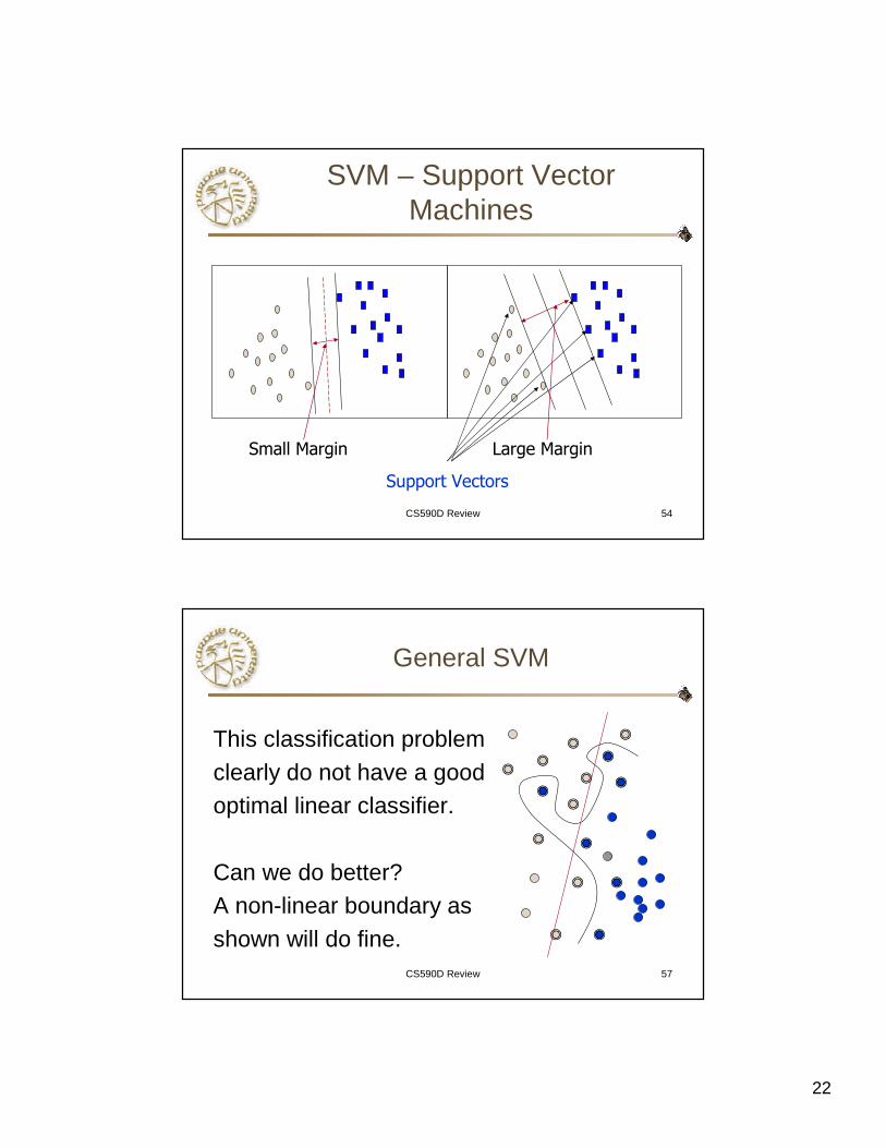
SVM – Support Vector Machines

Support Vectors

Small Margin Large Margin

CS590D Review 57

General SVM

This classification problemclearly do not have a goodoptimal linear classifier.

Can we do better? A non-linear boundary as shown will do fine.

23

CS590D Review 59

Mapping

• Mapping– Need distances in H:

• Kernel Function:– Example:

• In this example, H is infinite-dimensional

: d HΦ ℝ ֏

( ) ( )i jx xΦ ⋅Φ( , ) ( ) ( )i j i jK x x x x= Φ ⋅Φ

2 2|| || / 2( , ) i jx x

i jK x x e σ− −=

CS590D Review 60

Example of polynomial kernel.

r degree polynomial:K(x,x’)=(1+<x,x’>)d.For a feature space with two inputs: x1,x2

and a polynomial kernel of degree 2.K(x,x’)=(1+<x,x’>)2

Letand , then K(x,x’)=<h(x),h(x’)>.

225

21423121 )(,)(,2)(,2)(,1)( xxhxxhxxhxxhxh =====

216 2)( xxxh =

24

CS590D Review 61

Regress Analysis and Log-Linear Models in Prediction

• Linear regression: Y = α + β X– Two parameters , α and β specify the line and are to

be estimated by using the data at hand.– using the least squares criterion to the known values

of Y1, Y2, …, X1, X2, ….• Multiple regression: Y = b0 + b1 X1 + b2 X2.

– Many nonlinear functions can be transformed into the above.

• Log-linear models:– The multi-way table of joint probabilities is

approximated by a product of lower-order tables.– Probability: p(a, b, c, d) = αab βacχad δbcd

CS590D Review 62

Bagging and Boosting

• General idea Training data

Altered Training data

Altered Training data……..

Aggregation ….

Classifier CClassification method (CM)

CM

Classifier C1

CM

Classifier C2

Classifier C*

25

CS590D Review 63

Clustering

• Dissimilarity/Similarity metric: Similarity is expressed in terms of a distance function, which is typically metric:

d(i, j)• There is a separate “quality” function that measures the

“goodness” of a cluster.• The definitions of distance functions are usually very

different for interval-scaled, boolean, categorical, ordinal and ratio variables.

• Weights should be associated with different variables based on applications and data semantics.

• It is hard to define “similar enough” or “good enough”– the answer is typically highly subjective.

CS590D Review 64

Similarity and Dissimilarity Between Objects

• Distances are normally used to measure the similarity or dissimilarity between two data objects

• Some popular ones include: Minkowski distance:

where i = (xi1, xi2, …, xip) and j = (xj1, xj2, …, xjp) are two p-dimensional data objects, and q is a positive integer

• If q = 1, d is Manhattan distance

qq

pp

qq

jx

ix

jx

ix

jx

ixjid )||...|||(|),(

2211−++−+−=

||...||||),(2211 pp jxixjxixjxixjid −++−+−=

26

CS590D Review 65

Binary Variables

• A contingency table for binary data

• Simple matching coefficient (invariant, if the binary variable is

symmetric):

• Jaccard coefficient (noninvariant if the binary variable is

asymmetric):

dcbacb jid

++++=),(

pdbcasum

dcdc

baba

sum

++++

0

1

01

cbacb jid++

+=),(

Object i

Object j

CS590D Review 66

The K-Means Clustering Method

0

1

2

3

4

5

6

7

8

9

10

0 1 2 3 4 5 6 7 8 9 100

1

2

3

4

5

6

7

8

9

10

0 1 2 3 4 5 6 7 8 9 10

0

1

2

3

4

5

6

7

8

9

10

0 1 2 3 4 5 6 7 8 9 10

0

1

2

3

4

5

6

7

8

9

10

0 1 2 3 4 5 6 7 8 9 10

0

1

2

3

4

5

6

7

8

9

10

0 1 2 3 4 5 6 7 8 9 10

K=2

Arbitrarily choose K object as initial cluster center

Assign each objects to most similar center

Update the cluster means

Update the cluster means

reassignreassign

27

CS590D Review 67

The K-Medoids Clustering Method

• Find representative objects, called medoids, in clusters

• PAM (Partitioning Around Medoids, 1987)

– starts from an initial set of medoids and iteratively replaces one of the

medoids by one of the non-medoids if it improves the total distance of

the resulting clustering

– PAM works effectively for small data sets, but does not scale well for

large data sets

• CLARA (Kaufmann & Rousseeuw, 1990)

• CLARANS (Ng & Han, 1994): Randomized sampling

• Focusing + spatial data structure (Ester et al., 1995)

CS590D Review 68

Hierarchical Clustering

• Use distance matrix as clustering criteria. This method does not require the number of clusters k as an input, but needs a termination condition

Step 0 Step 1 Step 2 Step 3 Step 4

b

d

c

e

a a b

d e

c d e

a b c d e

Step 4 Step 3 Step 2 Step 1 Step 0

agglomerative(AGNES)

divisive(DIANA)

28

CS590D Review 69

BIRCH (1996)• Birch: Balanced Iterative Reducing and Clustering using Hierarchies,

by Zhang, Ramakrishnan, Livny (SIGMOD’96)

• Incrementally construct a CF (Clustering Feature) tree, a hierarchical data structure for multiphase clustering

– Phase 1: scan DB to build an initial in-memory CF tree (a multi-level compression of the data that tries to preserve the inherent clustering structure of the data)

– Phase 2: use an arbitrary clustering algorithm to cluster the leaf nodes of the CF-tree

• Scales linearly: finds a good clustering with a single scan and improves the quality with a few additional scans

• Weakness: handles only numeric data, and sensitive to the order of the data record.

CS590D Review 70

Density-Based Clustering Methods

• Clustering based on density (local cluster criterion), such as density-connected points

• Major features:– Discover clusters of arbitrary shape– Handle noise– One scan– Need density parameters as termination condition

• Several interesting studies:– DBSCAN: Ester, et al. (KDD’96)– OPTICS: Ankerst, et al (SIGMOD’99).– DENCLUE: Hinneburg & D. Keim (KDD’98)– CLIQUE: Agrawal, et al. (SIGMOD’98)

29

CS590D Review 71

CLIQUE: The Major Steps

• Partition the data space and find the number of points that lie inside each cell of the partition.

• Identify the subspaces that contain clusters using the Apriori principle

• Identify clusters:– Determine dense units in all subspaces of interests– Determine connected dense units in all subspaces of interests.

• Generate minimal description for the clusters– Determine maximal regions that cover a cluster of connected

dense units for each cluster– Determination of minimal cover for each cluster

CS590D Review 72

COBWEB Clustering Method

A classification tree

30

CS590D Review 73

Self-organizing feature maps (SOMs)

• Clustering is also performed by having several units competing for the current object

• The unit whose weight vector is closest to the current object wins

• The winner and its neighbors learn by having their weights adjusted

• SOMs are believed to resemble processing that can occur in the brain

• Useful for visualizing high-dimensional data in 2-or 3-D space

CS590D Review 74

Data Generalization and Summarization-based Characterization

• Data generalization– A process which abstracts a large set of task-

relevant data in a database from a low conceptual levels to higher ones.

– Approaches:• Data cube approach(OLAP approach)• Attribute-oriented induction approach

1

2

3

4

5

Conceptual levels

31

CS590D Review 75

Characterization: Data Cube Approach

• Data are stored in data cube• Identify expensive computations

– e.g., count( ), sum( ), average( ), max( )

• Perform computations and store results in data cubes

• Generalization and specialization can be performed on a data cube by roll-up and drill-down

• An efficient implementation of data generalization

CS590D Review 76

A Sample Data CubeTotal annual salesof TVs in U.S.A.Date

Prod

uct

Cou

ntrysum

sumTV

VCRPC

1Qtr 2Qtr 3Qtr 4Qtr

U.S.A

Canada

Mexico

sum

32

CS590D Review 77

Iceberg Cube

• Computing only the cuboid cells whose countor other aggregates satisfying the condition:

HAVING COUNT(*) >= minsup

• Motivation– Only a small portion of cube cells may be “above the water’’ in a

sparse cube

– Only calculate “interesting” data—data above certain threshold

– Suppose 100 dimensions, only 1 base cell. How many aggregate (non-base) cells if count >= 1? What about count >= 2?

CS590D Review 78

Top-k Average

• Let (*, Van, *) cover 1,000 records– Avg(price) is the average price of those 1000 sales

– Avg50(price) is the average price of the top-50 sales (top-50 according to the sales price

• Top-k average is anti-monotonic– The top 50 sales in Van. is with avg(price) <= 800 �

the top 50 deals in Van. during Feb. must be with avg(price) <= 800

………………

PriceCostProdCust_gr

pCityMonth

33

What is Concept Description?

• Descriptive vs. predictive data mining– Descriptive mining: describes concepts or task-

relevant data sets in concise, summarative, informative, discriminative forms

– Predictive mining: Based on data and analysis, constructs models for the database, and predicts the trend and properties of unknown data

• Concept description: – Characterization: provides a concise and succinct

summarization of the given collection of data– Comparison: provides descriptions comparing two or

more collections of data

Attribute-Oriented Induction: Basic Algorithm

• InitialRel: Query processing of task-relevant data, deriving the initial relation.

• PreGen: Based on the analysis of the number of distinct values in each attribute, determine generalization plan for each attribute: removal? or how high to generalize?

• PrimeGen: Based on the PreGen plan, perform generalization to the right level to derive a “prime generalized relation”, accumulating the counts.

• Presentation: User interaction: (1) adjust levels by drilling, (2) pivoting, (3) mapping into rules, cross tabs, visualization presentations.

34

Class Characterization:An Example

Name Gender Major Birth-Place Birth_date Residence Phone # GPA

JimWoodman

M CS Vancouver,BC,Canada

8-12-76 3511 Main St.,Richmond

687-4598 3.67

ScottLachance

M CS Montreal, Que,Canada

28-7-75 345 1st Ave.,Richmond

253-9106 3.70

Laura Lee…

F…

Physics…

Seattle, WA, USA…

25-8-70…

125 Austin Ave.,Burnaby…

420-5232…

3.83…

Removed Retained Sci,Eng,Bus

Country Age range City Removed Excl,VG,..

Gender Major Birth_region Age_range Residence GPA Count

M Science Canada 20-25 Richmond Very-good 16 F Science Foreign 25-30 Burnaby Excellent 22 … … … … … … …

Birth_Region

GenderCanada Foreign Total

M 16 14 30

F 10 22 32

Total 26 36 62

Prime Generalized Relation

Initial Relation

CS590D Review 82

Example: Analytical Characterization (cont’d)

• 1. Data collection– target class: graduate student– contrasting class: undergraduate student

• 2. Analytical generalization using Ui– attribute removal

• remove name and phone#

– attribute generalization• generalize major, birth_place, birth_date and gpa• accumulate counts

– candidate relation: gender, major, birth_country, age_range and gpa

35

83

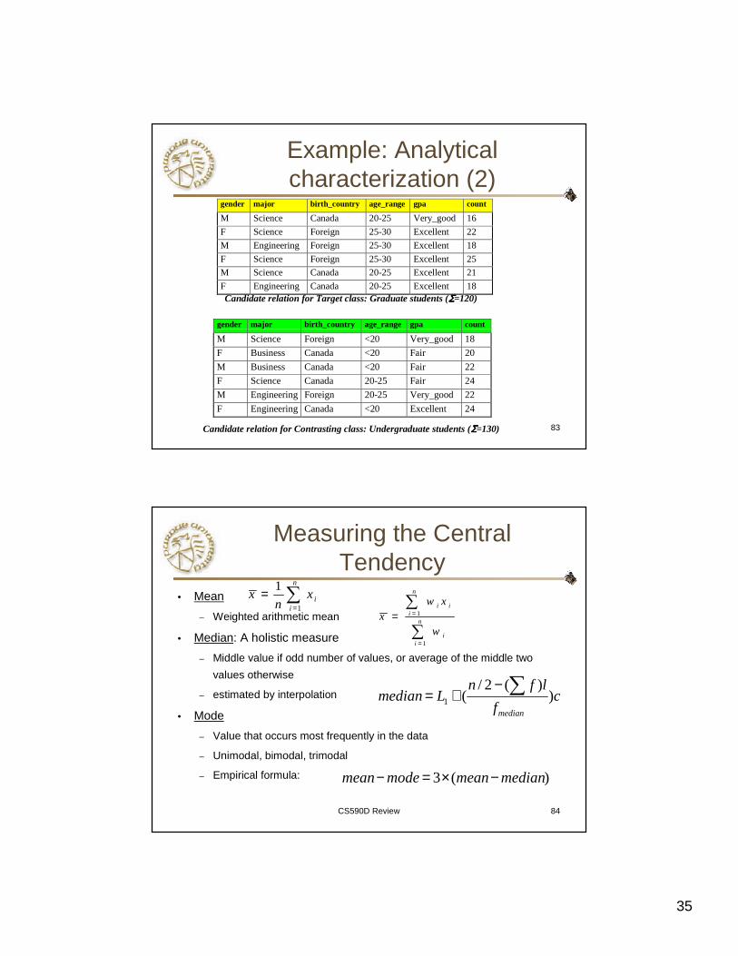
Example: Analytical characterization (2)

gender major birth_country age_range gpa count

M Science Canada 20-25 Very_good 16

F Science Foreign 25-30 Excellent 22

M Engineering Foreign 25-30 Excellent 18

F Science Foreign 25-30 Excellent 25

M Science Canada 20-25 Excellent 21

F Engineering Canada 20-25 Excellent 18Candidate relation for Target class: Graduate students (ΣΣΣΣ=120)

gender major birth_country age_range gpa count

M Science Foreign <20 Very_good 18

F Business Canada <20 Fair 20

M Business Canada <20 Fair 22

F Science Canada 20-25 Fair 24

M Engineering Foreign 20-25 Very_good 22

F Engineering Canada <20 Excellent 24

Candidate relation for Contrasting class: Undergraduate students (ΣΣΣΣ=130)

CS590D Review 84

Measuring the Central Tendency

• Mean

– Weighted arithmetic mean

• Median: A holistic measure

– Middle value if odd number of values, or average of the middle two

values otherwise

– estimated by interpolation

• Mode

– Value that occurs most frequently in the data

– Unimodal, bimodal, trimodal

– Empirical formula:

∑=

=n

iix

nx

1

1

∑

∑

=

==n

ii

n

iii

w

xwx

1

1

cf

lfnLmedian

median

))(2/

(1∑−

+=

)(3 medianmeanmodemean −×=−

36

CS590D Review 85

Measuring the Dispersion of Data

• Quartiles, outliers and boxplots

– Quartiles: Q1 (25th percentile), Q3 (75th percentile)

– Inter-quartile range: IQR = Q3 – Q1

– Five number summary: min, Q1, M, Q3, max

– Boxplot: ends of the box are the quartiles, median is marked, whiskers,and plot outlier individually

– Outlier: usually, a value higher/lower than 1.5 x IQR

• Variance and standard deviation

– Variance s2: (algebraic, scalable computation)

– Standard deviation s is the square root of variance s2

∑ ∑∑= ==

−−

=−−

=n

i

n

iii

n

ii x

nx

nxx

ns

1 1

22

1

22 ])(1

[1

1)(

1

1

CS590D Review 86

Test Taking Hints

• Open book/notes– Pretty much any non-electronic aid allowed

• Comprehensive– Must demonstrate you “know how to put it all

together”

• Time will be tight– Suggested “time on question” provided