cs599: convex and combinatorial optimization fall …shaddin/cs599fa13/slides/lec1.pdf · cs599:...
TRANSCRIPT
CS599: Convex and Combinatorial OptimizationFall 2013
Lecture 1: Introduction to Optimization
Instructor: Shaddin Dughmi

Outline
1 Course Overview
2 Administrivia
3 Linear Programming

Outline
1 Course Overview
2 Administrivia
3 Linear Programming
Mathematical OptimizationThe task of selecting the “best” configuration of a set of variables froma “feasible” set of configurations.
minimize (or maximize) f(x)subject to x ∈ X
Terminology: decision variable(s), objective function, feasible set,optimal solution, optimal valueTwo main classes: continuous and combinatorial
Course Overview 1/29
Continuous Optimization ProblemsOptimization problems where feasible set X is a connected subset ofEuclidean space, and f is a continuous function.
Instances typically formulated as follows.
minimize f(x)subject to gi(x) ≤ bi, for i ∈ C.
Objective function f : Rn → R.Constraint functions gi : Rn → R. The inequality gi(x) ≤ bi is thei’th constraint.In general, intractable to solve efficiently (NP hard)
Course Overview 2/29
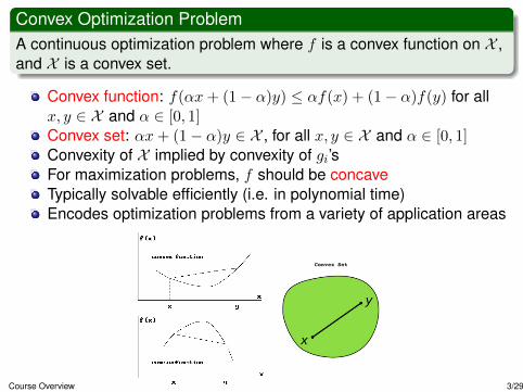
Convex Optimization ProblemA continuous optimization problem where f is a convex function on X ,and X is a convex set.
Convex function: f(αx+ (1− α)y) ≤ αf(x) + (1− α)f(y) for allx, y ∈ X and α ∈ [0, 1]Convex set: αx+ (1− α)y ∈ X , for all x, y ∈ X and α ∈ [0, 1]Convexity of X implied by convexity of gi’sFor maximization problems, f should be concaveTypically solvable efficiently (i.e. in polynomial time)Encodes optimization problems from a variety of application areas
Convex Set
Course Overview 3/29
Convex Optimization Example: Least SquaresRegression
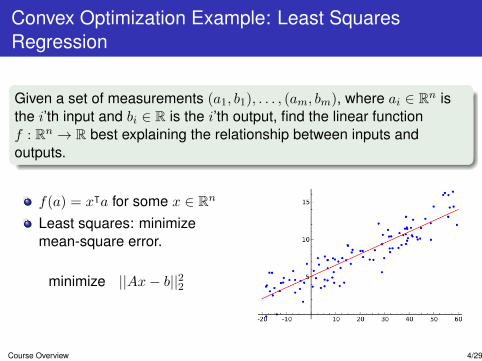
Given a set of measurements (a1, b1), . . . , (am, bm), where ai ∈ Rn isthe i’th input and bi ∈ R is the i’th output, find the linear functionf : Rn → R best explaining the relationship between inputs andoutputs.
f(a) = xᵀa for some x ∈ Rn
Least squares: minimizemean-square error.
minimize ||Ax− b||22
Course Overview 4/29
Convex Optimization Example: Minimum Cost Flow
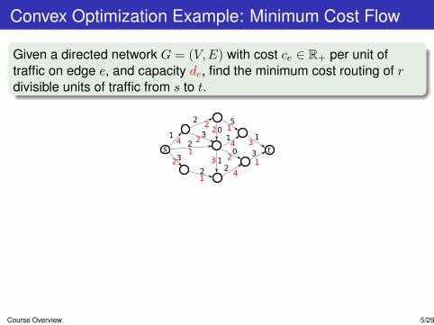
Given a directed network G = (V,E) with cost ce ∈ R+ per unit oftraffic on edge e, and capacity de, find the minimum cost routing of rdivisible units of traffic from s to t.
s t
1 11
2
2 2
2
3
330
50
1
1
1
1
1
22
2
2
4
4
3
3
4
2
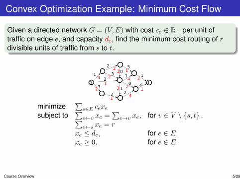
minimize∑
e∈E cexesubject to
∑e←v xe =
∑e→v xe, for v ∈ V \ {s, t} .∑
e←s xe = rxe ≤ de, for e ∈ E.xe ≥ 0, for e ∈ E.
Generalizes to traffic-dependent costs. For examplece(xe) = aex
2e + bexe + ce.
Course Overview 5/29
Convex Optimization Example: Minimum Cost Flow
Given a directed network G = (V,E) with cost ce ∈ R+ per unit oftraffic on edge e, and capacity de, find the minimum cost routing of rdivisible units of traffic from s to t.
s t
1 11
2
2 2
2
3
330
50
1
1
1
1
1
22
2
2
4
4
3
3
4
2
minimize∑
e∈E cexesubject to
∑e←v xe =
∑e→v xe, for v ∈ V \ {s, t} .∑
e←s xe = rxe ≤ de, for e ∈ E.xe ≥ 0, for e ∈ E.
Generalizes to traffic-dependent costs. For examplece(xe) = aex
2e + bexe + ce.
Course Overview 5/29
Combinatorial Optimization
Combinatorial Optimization ProblemAn optimization problem where the feasible set X is finite.
e.g. X is the set of paths in a network, assignments of tasks toworkers, etc...Again, NP-hard in general, but many are efficiently solvable (eitherexactly or approximately)
Course Overview 6/29
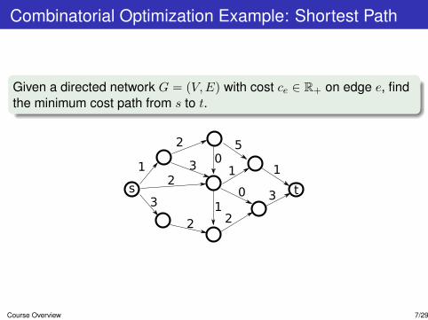
Combinatorial Optimization Example: Shortest Path
Given a directed network G = (V,E) with cost ce ∈ R+ on edge e, findthe minimum cost path from s to t.
s t
1 11
2
2 2
2
3
330
50
1
Course Overview 7/29
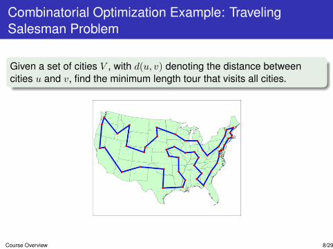
Combinatorial Optimization Example: TravelingSalesman Problem
Given a set of cities V , with d(u, v) denoting the distance betweencities u and v, find the minimum length tour that visits all cities.
Course Overview 8/29
Continuous vs Combinatorial Optimization
Some optimization problems are best formulated as one or theotherMany problems, particularly in computer science and operationsresearch, can be formulated as bothThis dual perspective can lead to structural insights and betteralgorithms
Course Overview 9/29
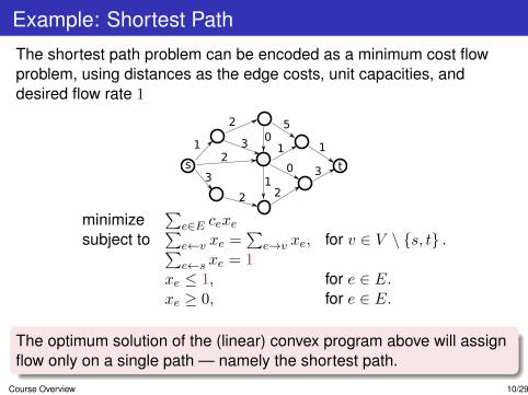
Example: Shortest Path
The shortest path problem can be encoded as a minimum cost flowproblem, using distances as the edge costs, unit capacities, anddesired flow rate 1
s t
1 11
2
2 2
2
3
330
50
1
minimize∑
e∈E cexesubject to
∑e←v xe =
∑e→v xe, for v ∈ V \ {s, t} .∑
e←s xe = 1xe ≤ 1, for e ∈ E.xe ≥ 0, for e ∈ E.
The optimum solution of the (linear) convex program above will assignflow only on a single path — namely the shortest path.
Course Overview 10/29
Course Goals
Recognize and model convex optimization problems, and developa general understanding of the relevant algorithms.Formulate combinatorial optimization problems as convexprogramsUse both the discrete and continuous perspectives to designalgorithms and gain structural insights for optimization problems
Course Overview 11/29
Who Should Take this Class
Anyone planning to do research in the design and analysis ofalgorithms
Convex and combinatorial optimization have become anindispensible part of every algorithmist’s toolkit
Students interested in theoretical machine learning and AIConvex optimization underlies much of machine learningSubmodularity has recently emerged as an important abstractionfor feature selection, active learning, planning, and otherapplications
Anyone else who solves or reasons about optimization problems:electrical engineers, control theorists, operations researchers,economists . . .
If there are applications in your field you would like to hear moreabout, let me know.
Course Overview 12/29
Course Outline
Weeks 1-4: Convex optimization basics and duality theoryWeek 5: Algorithms for convex optimizationWeeks 6-8: Viewing discrete problems as convex programs;structural and algorithmic implications.Weeks 9-14: Matroid theory, submodular optimization, and otherapplications of convex optimization to combinatorial problemsWeek 15: Project presentations (or additional topics)
Course Overview 13/29

Outline
1 Course Overview
2 Administrivia
3 Linear Programming
Basic Information
Lecture time: Tuesdays and Thursdays 2 pm - 3:20 pmLecture place: KAP 147Instructor: Shaddin Dughmi
Email: [email protected]: SAL 234Office Hours: TBD
Course Homepage: www.cs.usc.edu/people/shaddin/cs599fa13References: Convex Optimization by Boyd and Vandenberghe,and Combinatorial Optimization by Korte and Vygen. (Will placeon reserve)
Administrivia 14/29
Prerequisites
Mathematical maturity: Be good at proofsSubstantial exposure to algorithms or optimization
CS570 or equivalent, orCS303 and you did really well
Administrivia 15/29
Requirements and Grading
This is an advanced elective class, so grade is not the point.I assume you want to learn this stuff.
3-4 homeworks, 75% of grade.Proof based.Challenging.Discussion allowed, even encouraged, but must write up solutionsindependently.
Research project or final, 25% of grade. Project suggestions willbe posted on website.One late homework allowed, 2 days.
Administrivia 16/29

Survey
NameEmailDepartmentDegreeRelevant coursework/backgroundResearch project idea
Administrivia 17/29

Outline
1 Course Overview
2 Administrivia
3 Linear Programming
A Brief History
The forefather of convex optimization problems, and the mostubiquitous.Developed by Kantorovich during World War II (1939) for planningthe Soviet army’s expenditures and returns. Kept secret.Discovered a few years later by George Dantzig, who in 1947developed the simplex method for solving linear programsJohn von Neumann developed LP duality in 1947, and applied it togame theoryPolynomial-time algorithms: Ellipsoid method (Khachiyan 1979),interior point methods (Karmarkar 1984).
Linear Programming 18/29
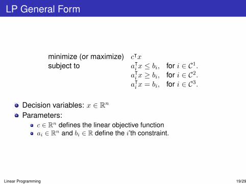
LP General Form
minimize (or maximize) cᵀxsubject to aᵀi x ≤ bi, for i ∈ C1.
aᵀi x ≥ bi, for i ∈ C2.aᵀi x = bi, for i ∈ C3.
Decision variables: x ∈ Rn
Parameters:c ∈ Rn defines the linear objective functionai ∈ Rn and bi ∈ R define the i’th constraint.
Linear Programming 19/29
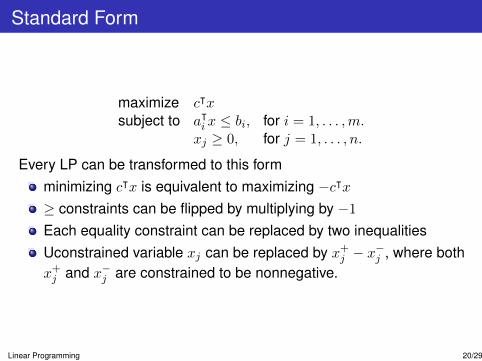
Standard Form
maximize cᵀxsubject to aᵀi x ≤ bi, for i = 1, . . . ,m.
xj ≥ 0, for j = 1, . . . , n.
Every LP can be transformed to this formminimizing cᵀx is equivalent to maximizing −cᵀx≥ constraints can be flipped by multiplying by −1Each equality constraint can be replaced by two inequalitiesUconstrained variable xj can be replaced by x+j − x
−j , where both
x+j and x−j are constrained to be nonnegative.
Linear Programming 20/29
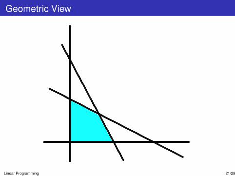
Geometric View
Linear Programming 21/29
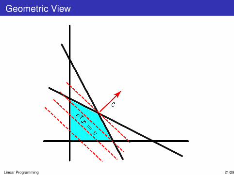
Geometric View
Linear Programming 21/29
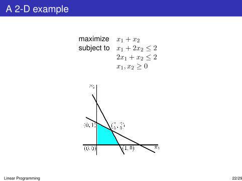
A 2-D example
maximize x1 + x2subject to x1 + 2x2 ≤ 2
2x1 + x2 ≤ 2x1, x2 ≥ 0
Linear Programming 22/29
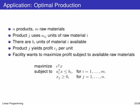
Application: Optimal Production
n products, m raw materialsProduct j uses aij units of raw material iThere are bi units of material i availableProduct j yields profit cj per unitFacility wants to maximize profit subject to available raw materials
maximize cᵀxsubject to aᵀi x ≤ bi, for i = 1, . . . ,m.
xj ≥ 0, for j = 1, . . . , n.
Linear Programming 23/29
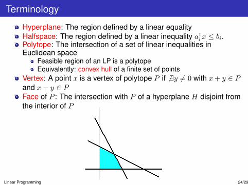
Terminology
Hyperplane: The region defined by a linear equalityHalfspace: The region defined by a linear inequality aᵀi x ≤ bi.Polytope: The intersection of a set of linear inequalities inEuclidean space
Feasible region of an LP is a polytopeEquivalently: convex hull of a finite set of points
Vertex: A point x is a vertex of polytope P if 6 ∃y 6= 0 with x+ y ∈ Pand x− y ∈ PFace of P : The intersection with P of a hyperplane H disjoint fromthe interior of P
Linear Programming 24/29
Basic Facts about LPs and Polytopes
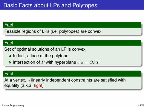
FactFeasible regions of LPs (i.e. polytopes) are convex
FactSet of optimal solutions of an LP is convex
In fact, a face of the polytopeintersection of P with hyperplane cᵀx = OPT
FactAt a vertex, n linearly independent constraints are satisfied withequality (a.k.a. tight)
Linear Programming 25/29
Basic Facts about LPs and Polytopes
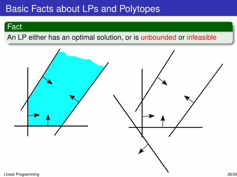
FactAn LP either has an optimal solution, or is unbounded or infeasible
Linear Programming 26/29
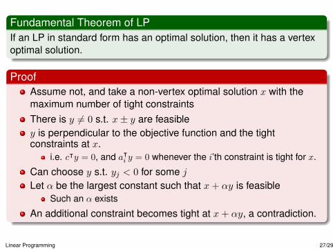
Fundamental Theorem of LPIf an LP in standard form has an optimal solution, then it has a vertexoptimal solution.
ProofAssume not, and take a non-vertex optimal solution x with themaximum number of tight constraintsThere is y 6= 0 s.t. x± y are feasibley is perpendicular to the objective function and the tightconstraints at x.
i.e. cᵀy = 0, and aᵀi y = 0 whenever the i’th constraint is tight for x.
Can choose y s.t. yj < 0 for some jLet α be the largest constant such that x+ αy is feasible
Such an α exists
An additional constraint becomes tight at x+ αy, a contradiction.
Linear Programming 27/29
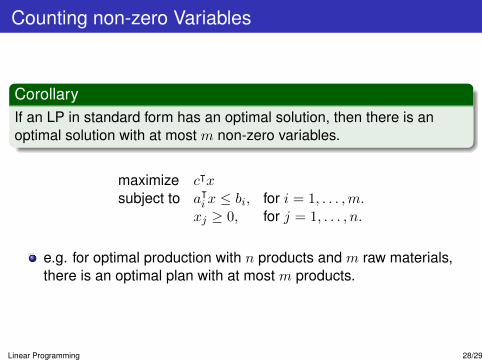
Counting non-zero Variables
CorollaryIf an LP in standard form has an optimal solution, then there is anoptimal solution with at most m non-zero variables.
maximize cᵀxsubject to aᵀi x ≤ bi, for i = 1, . . . ,m.
xj ≥ 0, for j = 1, . . . , n.
e.g. for optimal production with n products and m raw materials,there is an optimal plan with at most m products.
Linear Programming 28/29
Next Lecture
LP Duality and its interpretationsExamples of duality relationshipsImplications of Duality
Linear Programming 29/29