CS6402– Design and Analysis of Algorithm

16 marks Question & Answer

1. Explain algorithm specification

a. Pseudo code conventions 1. Comments begin with // and continue until the end of line.

1. Blocks are indicated and matching braces.: { and }. 2. An identifier begins with a letter 3. Assignment of values to variables is done using the assignment

statement <variable> := <expression> 4. There are two Boolean values true and false 5. Elements of multi dimensional array are accessed using [ and ]. 6. The following looping statements are employed: for, while and repeat – until. 7. A conditional statement has the following

forms: If <condition> then <statement>; 8. Input and output are done using the instructions read and write.

9. There only and one type of procedure: Algorithm An algorithm consists of heading and body. The heading takes the form

Algorithm Name <parameter list>

b. Recursive algorithms An algorithm is said to be recursive if the same algorithm is invoked in the body.

An algorithm that calls itself is Direct recursive. Algorithm A is said to be indeed recursive if it calls another algorithm, which in turn calls A.

2. Explain all asymptotic notations

Big oh The function f(n) = O(g(n)) iff there exist positive constants C and no such that

f(n)≤ C * g(n) for all n, n ≥n0.

Omega The function f(n) =Ω (g(n)) iff there exist positive constant C and no such that

f(n) C * g(n) for all n, n ≥ n0.

Theta

The function f(n) =θ (g(n)) iff there exist positive constant C1, C2, and no such

that C1 g(n)≤ f(n) ≤ C2 g(n) for all n, n ≥ n0.

Little oh The function f(n) = 0(g(n)) iff

Lim f(n) = 0 n - ∝ g(n)

Little Omega.

The function f(n) = ω (g(n)) iff

Lim f(n) = 0 n - ∝ g(n)

3. Explain binary search method

If „q‟ is always chosen such that „aq‟ is the middle element(that is, q=[(n+1)/2), then the resulting search algorithm is known as binary search.

Algorithm BinSearch(a,n,x) //Given an array a[1:n] of elements in nondecreasing // order, n>0, determine whether x is present

{ low : = 1; high : = n; while (low < high) do

{

mid : = [(low+high)/2];

if(x a[mid]) then high:= mid-1; else if (x a[mid]) then low:=mid

+ 1; else return mid; }

return 0;

} In conclusion we are now able completely describe the computing time of

binary search by giving formulas that describe the best, average and worst cases. Successful searches

θ(1) θ(logn) θ(Logn) best average worst

unsuccessful searches θ(logn)

best, average, worst

4. Explain the concepts of quick sort method and analyze its complexity

n quicksort, the division into subarrays is made so that the sorted subarrays do not need to be merged later.

Algorithm partition(a,m,p) {

v:=a[m];

I:=m; J:=p; Repeat { repeat I:=I+1; Until(a[I]>=v); Repeat J:=j-1; Until(a[j]<=v); If(I<j) then interchange(a,I,j); }until(I>=j);

a[m]:=a[j]; a[j]:=v; return j; }

Algorithm interchange(a,I,j) {

p:=a[I];

a[I]:=a[j]; a[j]:=p; }

Algorithm quichsort(p,q)

{ if(p<q) then

{ j:= partition(a,p,q+1); quicksort(p,j-1); quicksort(j+1,q); } } In analyzing QUICKSORT, we can only make the number of element

comparisions c(n). It is easy to see that the frequency count of other operations is of the same order as C(n).

5. Write the algorithm for finding the maximum and minimum and explain it.

The problem is to find the maximum and minimum items in a set of „n‟ elements. Though this problem may look so simple as to be contrived, it allows us to demonstrate divide-and-comquer in simple setting.

Algorithm straight MaxMin(a,n,max,min)

//set max to the maximum and min to the minimum of a[1:n] {

max := min: = a[i]; for i = 2 to n do

{ if(a[i] >max) then max: = a[i]; if(a[i] >min) then min: = a[i];

}

} Algorithm maxmin(I,j,max,min)

{ if( I = j) then max := min:=a[I]; else if(I=j-1) then { if(a[I]<a[j]) then {

max := a[j];min := a[I]; }

else { max:=a[I]; min := a[j];

} else

{ mid := [(I+j)/2];

maxmin(I,mid,max,min); maxmin(mid+1,j,max1,min1); if(max<max1) then max :=

max1; if(min>min1) then min:=min1;

}}

6. Explain the concept of merge sort

In merge sort, the elements are to be sorted in non-decreasing order. Given a sequence of n elements i.e. a [1], a [2]…. a [n], the general idea is to imagine them split into 2 sets a [1],

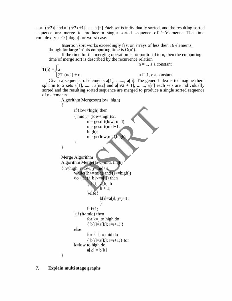
…a [(n/2)] and a [(n/2) +1], …. a [n].Each set is individually sorted, and the resulting sorted sequence are merge to produce a single sorted sequence of „n‟elements. The time complexity is O (nlogn) for worst case.

Insertion sort works exceedingly fast on arrays of less then 16 elements, though for large „n‟ its computing time is O(n

2).

If the time for the merging operation is proportional to n, then the computing time of merge sort is described by the recurrence relation

n = 1, a a constant

T(n) = a

2T (n/2) + n n 1, c a constant Given a sequence of elements a[1], ......., a[n]. The general idea is to imagine them

split in to 2 sets a[1], ......, a[n/2] and a[n/2 + 1], ......., a[n] each sets are individually sorted and the resulting sorted sequence are merged to produce a single sorted sequence of n elements.

Algorithm Mergesort(low, high) {

if (low<high) then { mid := (low+high)/2;

mergesort(low, mid); mergesort(mid+1, high); merge(low,mid,high)

}

}

Merge Algorithm

Algorithm Merge(low, mid, high) { h=high, i=low, j=mid+1;

while((h<=mid) and (j<=high)) do { if (a[h]<=a[j]) then

{ b[i]=a[h] h = h + 1;

}else{ b[i]=a[j], j=j+1; }

i=i+1; }if (h>mid) then

for k=j to high do

{ b[i]=a[k]; i=i+1; } else

for k=hto mid do { b[i]=a[k]; i=i+1;} for

k=low to high do a[k] = b[k]

} 7. Explain multi stage graphs

A multistage graph G = (V,E) is a directed graph in which the vertices are partitioned

into k>=2 disjoint sets Vi. The multistage graph problem is to find a minimum cost path from s to t.

Graph:-

Using the forward approach we

obtain Cost(i,j) = min{c(j,l)+cost(i+1,l)} Algorithm Fgraph(G,k,n,p) {

cost[n] := 0.0; for j := n-1 to 1 step –1 do

{ Let r be a vertex such that <j,r> is an edge of G and c[j,r] + cost[r] is

minimum; Cost[j]:= c[j,r]+cost[r]; d[j]:= r; }

p[1]:= 1; p[k]:=n; for j:= 2 to k-1 do p[j]:=d[p[j-1]];

}

From the backward approach we obtain

Bcost(i,j) = min{bcost(i-1,l)+c(l,j)}

Algorithm Bgraph(G,k,n,p) {

bcost[1]:= 0.0; for j := 2 to n do {

Let r be such that <r,j> is an edge of G and bcost[r]+c[r,j] is minimum; Bcost[j]:=bcost[r]+c[r,j]; D[j]:=r;

}

p[1]:= 1;

p[k]:= n; for j := k-1 to 2 do p[j]:= d[p[j+1]];

}

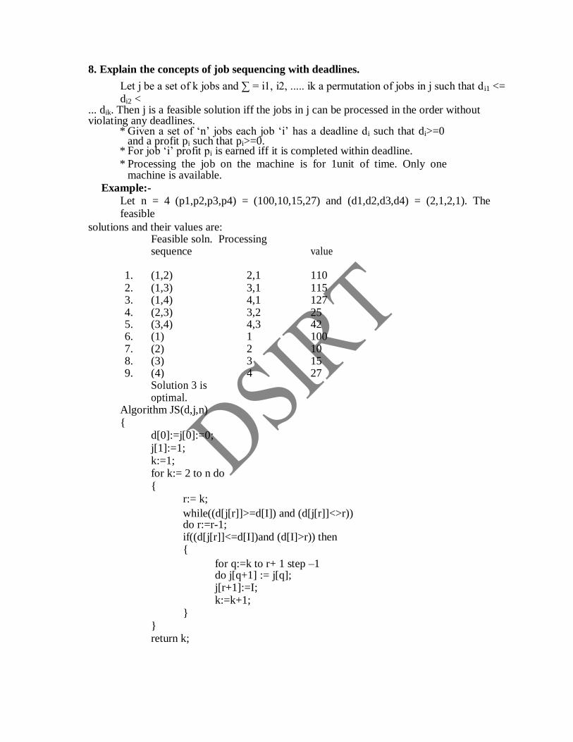
8. Explain the concepts of job sequencing with deadlines.

Let j be a set of k jobs and ∑ = i1, i2, ..... ik a permutation of jobs in j such that di1 <=

di2 < ... dik. Then j is a feasible solution iff the jobs in j can be processed in the order without violating any deadlines.

* Given a set of „n‟ jobs each job „i‟ has a deadline di such that di>=0 and a profit pi such that pi>=0.

* For job „i‟ profit pi is earned iff it is completed within deadline. * Processing the job on the machine is for 1unit of time. Only one

machine is available. Example:-

Let n = 4 (p1,p2,p3,p4) = (100,10,15,27) and (d1,d2,d3,d4) = (2,1,2,1). The

feasible

solutions and their values are:

Feasible soln. Processing sequence value

1. (1,2) 2,1 110 2. (1,3) 3,1 115 3. (1,4) 4,1 127 4. (2,3) 3,2 25 5. (3,4) 4,3 42 6. (1) 1 100 7. (2) 2 10 8. (3) 3 15 9. (4) 4 27

Solution 3 is optimal.

Algorithm JS(d,j,n)

{ d[0]:=j[0]:=0;

j[1]:=1; k:=1; for k:= 2 to n do

{

r:= k; while((d[j[r]]>=d[I]) and (d[j[r]]<>r)) do r:=r-1; if((d[j[r]]<=d[I])and (d[I]>r)) then {

for q:=k to r+ 1 step –1 do j[q+1] := j[q]; j[r+1]:=I; k:=k+1;

}

} return k;

} For job sequence there are two possible parameters in terms of which its complexity

can be measured. We can use n the number of jobs, and s, the number of jobs included in the solution j. If we consider the job set pi = di = n – I + 1, 1 <= I <= n, the algorithm takes φ(n

2) time to determine j. Hence the worst case computing time for job sequence is φ(n

2)

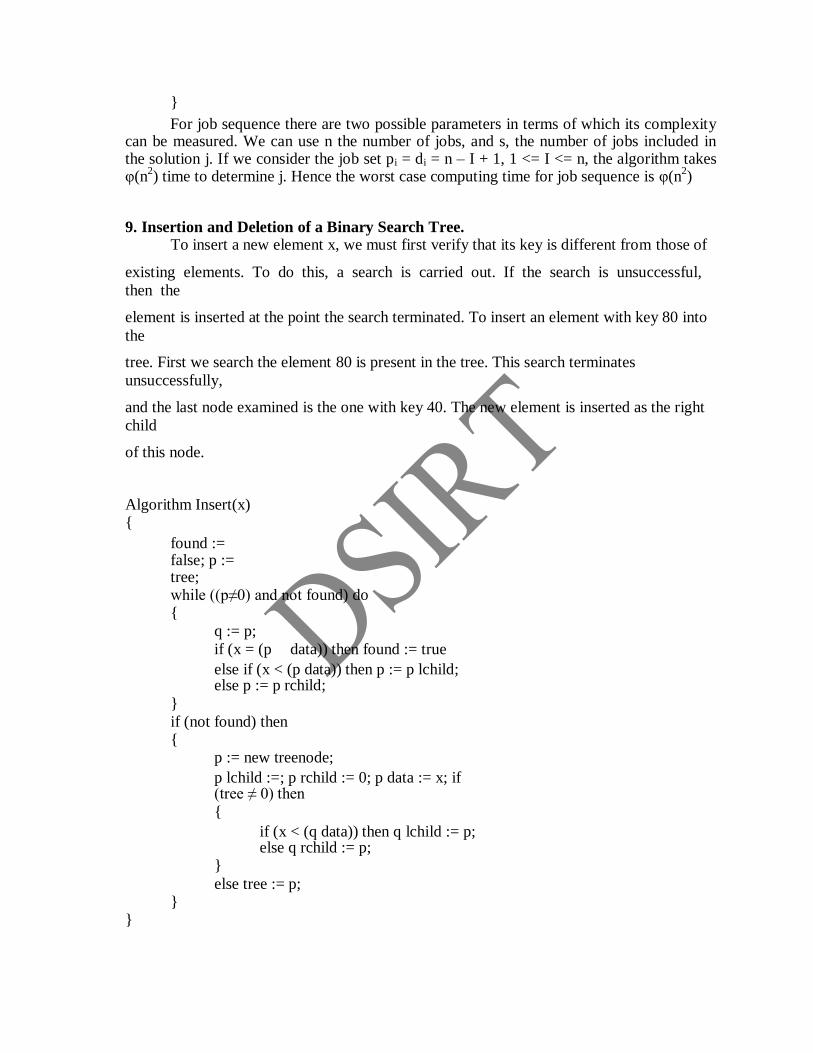
9. Insertion and Deletion of a Binary Search Tree. To insert a new element x, we must first verify that its key is different from those of

existing elements. To do this, a search is carried out. If the search is unsuccessful,

then the element is inserted at the point the search terminated. To insert an element with key 80 into

the tree. First we search the element 80 is present in the tree. This search terminates

unsuccessfully, and the last node examined is the one with key 40. The new element is inserted as the right

child of this node.

Algorithm Insert(x) {

found := false; p := tree; while ((p≠0) and not found) do {

q := p;

if (x = (p data)) then found := true else if (x < (p data)) then p := p lchild; else p := p rchild;

}

if (not found) then {

p := new treenode; p lchild :=; p rchild := 0; p data := x; if (tree ≠ 0) then {

if (x < (q data)) then q lchild := p; else q rchild := p;

}

else tree := p; }

}

b) Deletion from a binary tree.

To delete an element from the tree, the left child of its parent is set to 0 and the node disposed. To delete the 80 from this tree, the right child field of 40 is set to 0. Then the node containing 80 is disposed. The deletion of a nonleaf element that has only one child is also

easy. The node containing the element to be deleted is disposed, and the single child takes the

place of the disposed node. To delete another element from the tree, simply change the

pointer from the parent node to the single child node. 10. Show that DFS and BFS visit all vertices in a connected graph G reachable from any one of vertices.

In the breadth first search we start at a vertex v and mark it as having been reached.

The vertex v is at this time said to be unexplored. A vertex is said to have been explored by an algorithm when the algorithm has visited all vertices adjacent from it. All unvisited

vertices adjacent from v are visited next. These are new unexplored vertices. Vertex v has now been explored. The newly visited vertices haven‟t been explored and are put onto the end of a list

of unexplored vertices. The first vertex on this list is the next to be explored. Exploration

continues until no unexplored vertex is left. Breadth first search

We start at a vertex V and mark it as have been reached. The vertex v is at this time said to be unexplorted. All visited vertices adjacent from v are visited next. If G is represented by its adjacent then the time is O(n2).

Algorithm BFS(v)

{

u := v;

visited[v] := 1;

repeat

{

for all vertices w adjacent from u do

{

if (visited[w] = 0) then

{

add w to q;

visited[w] := 1;

}

}

if q is empty then return;

delet u from q;

} until (false)

}

A depth first search of a graph differs from a breadth first search in that the

exploration of a vertex v is suspended as soon as a new vertex is reached. At this time the exploration of the new vertex u begins. When the new vertex has been

explored, the exploration of v continues.

Depth first search The exploration of a vertex V is suspended as soon as a new vertex is reached. Algorithm DFS(v)

Algoithm DFS(v) {

visited[v]:=1; for each vertex q adjacent from v do

{ if (visited[w] =0 ) then DFS(w);

} }

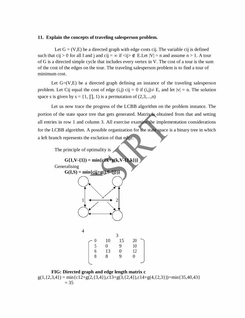
11. Explain the concepts of traveling salesperson problem.

Let G = (V,E) be a directed graph with edge costs cij. The variable cij is defined

such that cij > 0 for all I and j and cij = ∞ if <ij> ∉ E.Let |V| = n and assume n > 1. A tour

of G is a directed simple cycle that includes every vertex in V. The cost of a tour is the sum

of the cost of the edges on the tour. The traveling salesperson problem is to find a tour of

minimum cost.

Let G=(V,E) be a directed graph defining an instance of the traveling salesperson

problem. Let Cij equal the cost of edge (i,j) cij = 0 if (i,j)≠ E, and let |v| = n. The solution

space s is given by s = {1, ∏, 1) is a permutation of (2,3,...,n)

Let us now trace the progress of the LCBB algorithm on the problem instance. The

portion of the state space tree that gets generated. Matrix is obtained from that and setting

all entries in row 1 and column 3. All exercise examine the implementation considerations

for the LCBB algorithm. A possible organization for the state space is a binary tree in which

a left branch represents the exclution of that edge.

The principle of optimality is

G{1,V-{1}) = min{c1k+g(k,V-{1,k})}

Generalising

G(I,S) = min{cij+g(j,S-{j})}

1 2

4 3

0 10 15 20 5 0 9 10 6 13 0 12 8 8 9 0

FIG: Directed graph and edge length matrix c g(1,{2,3,4}) = min{c12+g(2,{3,4}),c13+g(3,{2,4}),c14+g(4,{2,3}))=min{35,40,43}

= 35

12. Explain all the techniques for binary trees

When the search necessarily involves the examination of every vertex in the object

being searched it is called a traversal. There are many operations that we want to perform on

binary trees. If we let L,D and R stand for moving left printing the data and moving right

when at a node then there are six possible combinations of traversal:

LDR,LRD,DLR,DRL,RDL and RLD. If we adopt the convention that we traverse left

before right then only three traversals remain: LDR,LRD and DLR. To these we assign the

names inorder, postorder and preorder.

Algorithm inorder(t)

{

if t ≠ 0 then {

inorder(t -> lchild); visit(t); inorder(t -> rchild);

} }

Algorithm preorder(t)

{

if t ≠ 0 then {

visit(t); preorder(t -> lchild); preorder(t -> rchild);

} }

Algorithm postorder(t)

{

if t ≠ 0 then {

postorder(t -> lchild); postorder(t -> rchild); visit(t);

} }

13. Write the Bellman and ford algorithm, and explain its concepts (10)

The recurrence for dist is given dist

k[u] = min{dist

k-1[u],mini{dist

k-1[i]+cost[i,u]}}

Graph:-

Algorithm BellmanFord(v,cost,dist,n)

{ for I:= 1 to n do dist[I] := cost[v,I]; for k:= 2 to n-1 do for each u such that u ≠v and u has at least one incoming edge do for each <I,u> in the graph do if dist[u]> dist[I]+cost[I,u] then dist[u] := dist[I]+cost[I,u];

}

The overall complexity is O(n3) when adjacency matrices are used and O(ne)

when adjacency lists are used.

14. Discuss the concepts of 8 – queens problem

The problem is to place eight queens on a 8 x 8 chessboard so that no two queen “attack” that is, so that no two of them are on the same row, column or on the diagonal.

One solution to the 8 queen problem

Q

Q

Q

Q

Q

Q

Q

Q

for j := 1 to k-1 do

if(x[j]=I) or(abs(x[j]-I)=abs(j-k))) then return false;

return true;

}

Algorithm Nqueens(k,n)

{

for I:= 1 to n do

{

if( place(k,I) then

{

x[k]:= I;

if(k=n) then write(x[1:n]);

Algorithm place(k,I)

{

else

Nqueens(k+1,n) } } }

15. Graph Coloring Techniques Let G be a graph and m be a positive integer. The nodes of G can be colored in

such a way that no two adjacent nodes have the same color yet only m colors are used.

This is termed by m-color ability decision problem and given it is the degree of the

queen graph, then it can be colored with j + 1 colors. The m – color ability optimization

problem asks for the smallest integer m for which the graph G can be colored.

b

a e

d c

In the fig the graph can be colored with three colors 1, 2 and 3. The color of each

node is indicated next to it. It can also be seen that three colors are needed to color this

graph and hence this graphs chromatic number is 3.

Suppose we represent a graph by its adjascency matrix G[1:n, 1:n], where G[I, j]

= 1; if [I, j] is an edge of G and G[I, j] = 0, otherwise the colors are represented by the

integer 1, 2, 3, …., n and solution are given by the n tupile.

(x1, x2, …., xn) where xi is the color of node is 1.

Algorithm mcoloring(k) {

repeat

{ if (x[k] = 0) then return; if (k = n) then write (x[1: n]); else mcoloring(k+1);

} until (false); }

16. Write and explain the concepts of 0/1 knapsack problem. A bag or sack is given capacity n and n objects are given. Each object has

weight

wi and profit pi .Fraction of object is considered as xi (i.e) 0<=xi<=1 .If fraction is 1

then entire object is put into sack. When we place this fraction into the sack we get wixi

and pixi.

The solution to the knapsack problem can be viewed as a result of sequence of

decisions. We have to decide the value of xi. xi is restricted to have the value 0 or 1

and by

using the function knap(l, j, y) we can represent the problem as

maximum Σpi xi

subject to Σwi xi <

y where l - iteration, j - number of objects, y – capacity

The formula to calculate optimal solution is

g0(m)=max{g1, g1(m-w1)+p1}.

Algorithm BKnap(k, cp, cw) {

if (cw + w[k] <= m) then

{

y[k] := 1; if (k < n) then BKnap(k+1, cp + p[k], cw + w[k]); if ((cp + p[k] > fp) and (k = n)) then {

fp := cp + p[k]; fw := cw + w[k]; for j := 1 to k do

x[j] := y[j]; }

}

if (bound (cp, cw, k) >= fp) then

{ y[k] := 0; if (k<n) then BKnap(k+1, cp, cw) if ((cp> fp) and (k = n) then {

fp := cp; fw := cw; for j := 1 to k do

x[j] := y[j]; }}}

17. Write and explain the techniques in branch and bound method

The searching techniques that are commonly used in Branch-and-Bound method are:

v. FIFO vi. LIFO vii. LC

viii. Heuristic search Control Abstraction for LC – Search

In both LIFO and FIFO branch and bound the selection rule for the next E – node is

rather rigid and in a sence blind. The selection rule for the next E – nod edoes not give any

preference to a node that has a very good chance of getting the search to an answer not

quickly.

The search for an answer node can often be speeded by using an intelligent ranking

function for live node. The next E – node is selected on the basis of ranking function.

Let t be a state space tree and c() a cost function for the nodes in t. If x is a node in t,

then c(x) is the minimum cost of any answer node in the subtree with root x. c(t) is the cost

of a minimum – cost answer in tree t. As remarked earlier, it is usually not possible to find

an easily computable function c(). The heuristic search should be easy to compute and

generally has the property that if x is either an answer node or a leaf node, then c(x) = C(x).

Listnode = record{ Listnode * next, *parent;

Float coast;

Algorithm LCSearch(t) {

if *t is an answer node then output *t and

return; E := t;

Initialize the list of live nodes to be empty;

Repeat

{

for each child x of E do

{

18. Non deterministic Algorithm Algorithm has the property that the result of every operation whose outcome are not

uniquely defined. The machine executing such operation is allowed to choose any one of these outcomes. To specify such algorithms, introduce three new functions.

Choice (s) – Choose any one of the element of the set s. Failure () – Signals an unsuccessful completion

Success () – Signals a successful completion.

The assignment statement x: = choice(1, n) could result in x being assigned any one

of the integer in the range[1, n]. The failure() and Success() signals are used to define a computation of the algorithm. The set of choices that leads to a successful completion, then one such set of choice is always made and the algorithm terminates successfully.

Consider the problem of searching for an element x in a set of elements A[1, n]

where n>= 1.

Step 1: J: = choice (1, n); Step 2: If A[j] = x then

Write (j); Success()

; Step 3: (A[j] != x) Write(0);

Failure();

19. NP – hard Graph Problems 1. Pick a problem L1 already known to be NP – hard. 2. Show how to obtain an instance I‟ of L2 from any Instance I of L1, Such that

from the solution of I‟ we can determine the solution to instance I of L1. 3. Conclude from step 2 that L1 α L2. 4. From step1 and step 3, the transitivity of α that L2 is NP – hard

a) Clique Decision Problem (CDP)

A maximal complete sub graph of a graph G = (V, E) is a clique. The size of the

clique is the number of vertices in it. The Max clique problem is an optimization problem

that has to determine the size of a largest clique in G. The corresponding decision problem

is to determine wheather G has a clique of size k for some k.

The Input to the max clique decision problem can be provided as a sequence of

edged and an integer k. Each edge in E(G) is a pair of numbers(I, j). The size of the input for

each edge(I, j) is log I 2 + log j 2 + 2. if a binary representation is assumed. The input size

of any instance is

b) Node Cover Decision problem

A set V is a node cover for a graph G = (V, E) iff all edges in E are incident to atleast one vertex in s. The size [s] of the cover is the number of vertices in s. c) Chromatic Number Decision Problem. (CNDP)

A coloring of a graph G = (V, E) is a function f: {1, 2, ….., k} defined for all x € v. If (V, E) € E, then f(u) ≠ f(v).

d) NP – hard scheduling problem This problem requires us to decided whether a given multiset A = {a1, a2, a3,

….., an) of n positive integer has a partition p. such that e) Job shop scheduling.

A job shop like a flow shop has m different processors. The n job to be scheduled require the completion of several task. The time of the j

th task for job ji.

The task for any job ji are to be carried out in the order 1, 2, 3, ….. and so on

20. Approximation & ε - Approximation Algorithms

• A is an absolute approximation algorithm for problem p iff for every

instance I of p.

f * (I ) − f (I ) ≤ k for some constant k.

A is an f(n)

approximate algorithm iff for every instance I of size

n,

f * (I ) − f (I ) ≤ f (n) for p*(I) > 0.

An ε - Approximation algorithm is an f(n) approximate algorithm for which f(n) <= ε for some constant e.

A(e) is an approximation scheme iff for every given ε > 0 and problem

instance I, A(e)

generate α feasible solution such

that

f * (I ) − f

(I )

≤ e where f*(I) >

0.

f * (I )

• An approximation scheme is a polynomial time approximation scheme iff for every fixed e > 0 it has a computing time ie, a polynomial in the problem size.

• An approximation scheme whose computing time is a polynomial both in

the problem size s in 1/e is a fully polynomial time approximation scheme.

Maximum program stored problem Assume we have n programs and two storage device. let li be the

amount of storage needed to store the ith program. Let L be the storage

capacity of each disk. Determine the maximum number of these n programs that can be stored on two desk is NP – hard

i) Partition of maximum program ii) Let I be any instance of the maximum programs stored problem. Let

f*(I) be the maximum number of programs that can be stored on two

desks each of length L .