cs6716 pattern recognitioncc.gatech.edu/~afb/classes/cs7616-spring2014/slides/cs... ·...
TRANSCRIPT

Boosting and Ensembles CS7616 Pattern Recognition – A. Bobick
Aaron Bobick School of Interactive Computing
CS6716 Pattern Recognition Ensembles and Boosting (1)

Boosting and Ensembles CS7616 Pattern Recognition – A. Bobick
Administrivia • Chapter 10 of the Hastie book. • Slides brought to you by Aarti Singh, Peter Orbanz, and
friends. • Slides posted…sorry that took so long… • Final project discussion…

Boosting and Ensembles CS7616 Pattern Recognition – A. Bobick
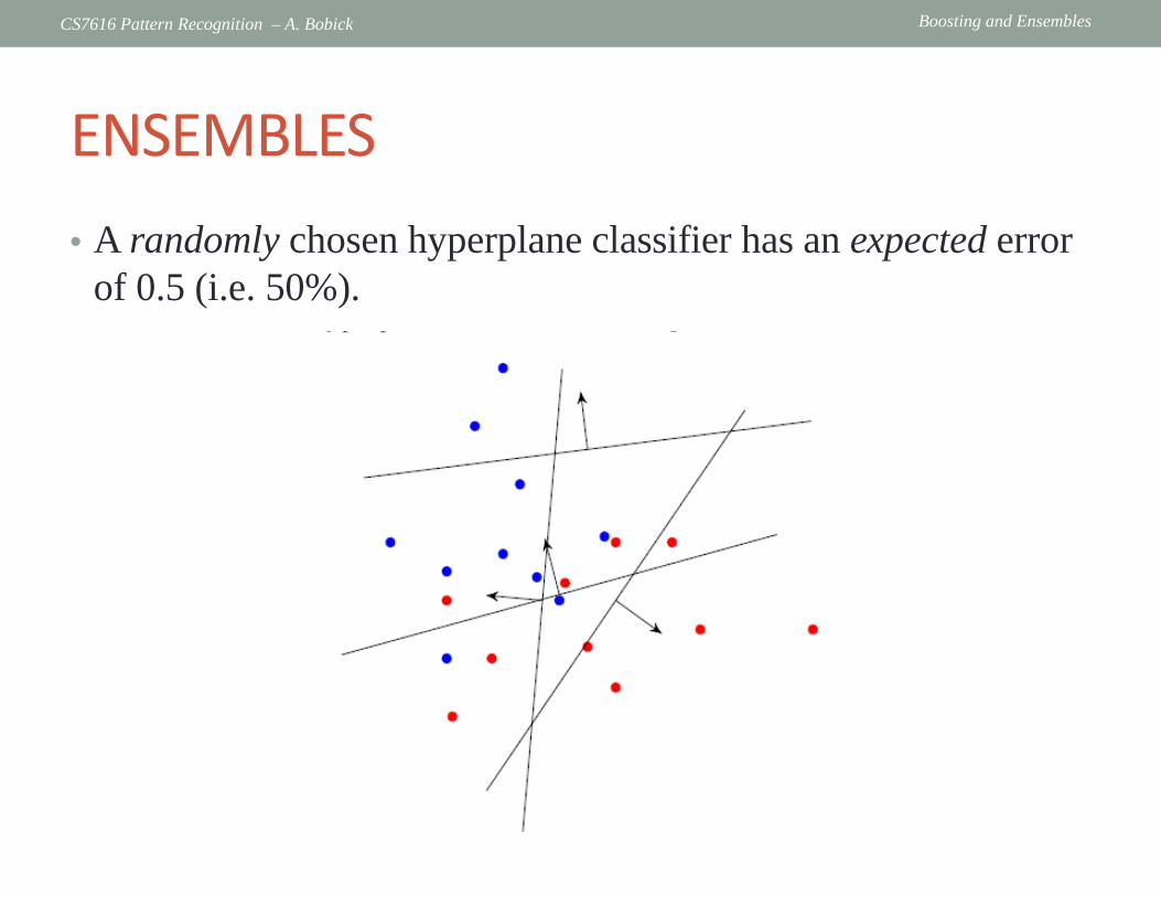
ENSEMBLES • A randomly chosen hyperplane classifier has an expected error
of 0.5 (i.e. 50%).
Boosting and Ensembles CS7616 Pattern Recognition – A. Bobick
ENSEMBLES • A randomly chosen hyperplane classifier has an expected error
of 0.5 (i.e. 50%).

Boosting and Ensembles CS7616 Pattern Recognition – A. Bobick
Ensembles • Many random hyperplanes combined by majority vote: Still
0.5 • A single classifier slightly better than random: 0.5 + ε. • What if we use m such classifiers and take a majority vote?
146 / 531

Boosting and Ensembles CS7616 Pattern Recognition – A. Bobick
Voting • Decision by majority vote
• m individuals (or classifiers) take a vote. m is an odd number. • They decide between two choices; one is correct, one is wrong. • After everyone has voted, a decision is made by simple majority.
• Note: For two-class classifiers 𝑓𝑓1, … , 𝑓𝑓𝑚𝑚 (with output ±1):
majority vote = 𝑠𝑠𝑠𝑠𝑠𝑠 �𝑓𝑓𝑗𝑗
𝑚𝑚
𝑗𝑗=1

Boosting and Ensembles CS7616 Pattern Recognition – A. Bobick
Voting – likelihoods • We make some simplifying assumptions: • Each individual makes the right choice with probability
𝑝𝑝 ∈ 0, 1
• The votes are independent, i.e. stochastically independent when regarded as random outcomes.
• Given n voters, the probability the majority makes the right choice:
• This formula is known as Condorcet’s jury theorem
147 / 531
12
!Pr(majority correct)!(
(1 ))!
m
j
j jm
mpm p
j m j−
+=
−∑−

Boosting and Ensembles CS7616 Pattern Recognition – A. Bobick
Power of weak classifiers
12
!Pr(majority correct)!(
(1 ))!
m
j
j jm
mpm p
j m j−
+=
−∑−

Boosting and Ensembles CS7616 Pattern Recognition – A. Bobick
ENSEMBLE METHODS • An ensemble method makes a prediction by combining the
predictions of many classifiers into a single vote. • The individual classifiers are usually required to perform only
slightly better than random. For two classes, this means slightly more than 50% of the data are classified correctly. Such a classifier is called a weak learner.
149 / 531

Boosting and Ensembles CS7616 Pattern Recognition – A. Bobick
ENSEMBLE METHODS • From before: if the “weak learners” are random and
independent, the prediction accuracy of the majority vote will increase with the number of weak learners.
• But, since the weak learners are all typically trained on the same training data, producing random, independent weak learners is difficult. • (See later for random forests)
• Different ensemble methods (e.g. Boosting, Bagging, etc) use
different strategies to train and combine weak learners that behave relatively independently.
149 / 531

Boosting and Ensembles CS7616 Pattern Recognition – A. Bobick
Making ensembles work • Boosting (today)
• After training each weak learner, data is modified using weights. • Deterministic algorithm.
• Bagging (bootstrap aggregation from earlier)
• Each weak learner is trained on a random subset of the data.
• Random forests (later)
• Bagging with tree classifiers as weak learners. • Uses an additional step to remove dimensions that carry little
information.
150 / 531

Boosting and Ensembles CS7616 Pattern Recognition – A. Bobick
Why boost weak learners?
Goal: Automatically categorize type of call requested (Collect, Calling card, Person--to--person, etc.)
• Easy to find “rules of thumb” that are “often” correct. E.g. If ‘card’ occurs in utterance, then predict ‘calling card’
• Hard to find single highly accurate prediction rule.

Boosting and Ensembles CS7616 Pattern Recognition – A. Bobick
• Simple (a.k.a. weak) learners e.g., naïve Bayes, logistic regression, decision stumps (or shallow decision trees)
Are good -- Low variance, don’t usually overfit Are bad -- High bias, can’t solve hard learning problems
• Can we make weak learners always good??? – No!!! But often yes…
Fighting the bias-‐variance tradeoff
Boosting and Ensembles CS7616 Pattern Recognition – A. Bobick
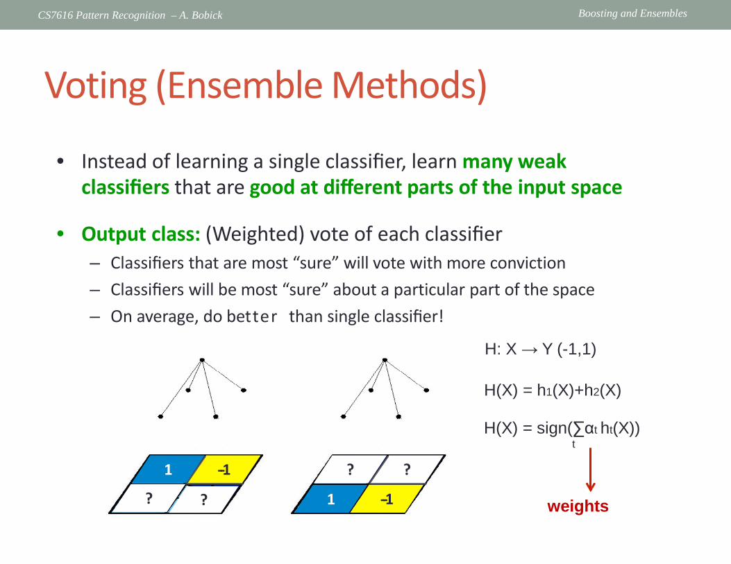
• Instead of learning a single classifier, learn many weak classifiers that are good at different parts of the input space
• Output class: (Weighted) vote of each classifier
– Classifiers that are most “sure” will vote with more conviction – Classifiers will be most “sure” about a particular part of the space – On average, do better than single classifier!
H: X → Y (-1,1) h1(X) h2(X)
H(X) = h1(X)+h2(X)
H(X) = sign(∑αt ht(X)) t
1 --1
? ?
? ?
1 --1 weights
Voting (Ensemble Methods)

Boosting and Ensembles CS7616 Pattern Recognition – A. Bobick
Voting (Ensemble Methods)
15
• Instead of learning a single classifier, learn many weak classifiers that are good at different parts of the input space
• Output class: (Weighted) vote of each classifier
– Classifiers that are most “sure” will vote with more conviction – Classifiers will be most “sure” about a par' cular part of the space – On average, do better than single classifier!
• But how do you ???
– force classifiers ℎ𝑡𝑡 to learn about different parts of the input space?
– weight the votes of different classifiers? 𝛼𝛼𝑡𝑡

Boosting and Ensembles CS7616 Pattern Recognition – A. Bobick
• Idea: given a weak learner, run it multiple times (reweighted) training data, then let learned classifiers vote
• On each iteration 𝑡𝑡 :
– weight each training example by "how incorrectly" it was classified
– Learn a weak hypothesis – ℎ𝑡𝑡 – A strength for this hypothesis – 𝛼𝛼𝑡𝑡
• Final classifier: 𝐻𝐻 𝑥𝑥 = 𝑠𝑠𝑠𝑠𝑠𝑠(Σ𝛼𝛼𝑡𝑡 ℎ𝑡𝑡 𝑥𝑥 )
• Practically useful AND Theoretically interesting
Boosting (Shapire, 1989)

Boosting and Ensembles CS7616 Pattern Recognition – A. Bobick
Learning from weighted data
17
• Consider a weighted dataset – D(i) – weight of i th training example 𝒙𝒙𝑖𝑖 ,𝑦𝑦𝑖𝑖 – Interpretations:
• i th training example counts as D(i) examples • If you were to “resample” data, you would get more samples of
“heavier” data points
• Now, in all calculations, whenever used, i th training example counts as D(i) “examples” – e.g., in MLE redefine Count(Y=y) to be weighted count
Unweighted data m
Count(Y=y) = ∑ 1(Y i=y) i =1
Weights D(i) Count(Y=y) = ∑ D(i)1(Y i=y)
i =1
m

Boosting and Ensembles CS7616 Pattern Recognition – A. Bobick
Boosting – weak learners

Boosting and Ensembles CS7616 Pattern Recognition – A. Bobick
AdaBoost.M1 (1)

Boosting and Ensembles CS7616 Pattern Recognition – A. Bobick
AdaBoost.M1 (2)

Boosting and Ensembles CS7616 Pattern Recognition – A. Bobick
Example sequence

/76
Boosting Iteratively reweighting training samples. Higher weights to previously misclassified samples.
22
1 round 2 rounds 3 rounds 4 rounds 5 rounds 50 rounds ICCV09 Tutorial Tae-Kyun Kim University of Cambridge

Boosting and Ensembles CS7616 Pattern Recognition – A. Bobick
Not mysterious????

Boosting and Ensembles CS7616 Pattern Recognition – A. Bobick
Minimizing a loss function

Boosting and Ensembles CS7616 Pattern Recognition – A. Bobick
Forward stage additive model

Boosting and Ensembles CS7616 Pattern Recognition – A. Bobick
Exponential loss (1)

Boosting and Ensembles CS7616 Pattern Recognition – A. Bobick
Exponential loss (2) • At each node/level:

Boosting and Ensembles CS7616 Pattern Recognition – A. Bobick

Boosting and Ensembles CS7616 Pattern Recognition – A. Bobick
Training error of final classifier is bounded by:
Convex upper bound
Where
exp loss If boosting can make upper bound → 0, then training error → 0
0/1 loss
1
Analyzing training error
29 0

Boosting and Ensembles CS7616 Pattern Recognition – A. Bobick
Why zero training error isn’t the end?!?!

Boosting and Ensembles CS7616 Pattern Recognition – A. Bobick
• Boosting often but not always, – Robust to overfitting – Test set error decreases even after training error is zero
[Schapire, 1989]
Test Error Training Error
Boosting results – Digit recognition
31

Boosting and Ensembles CS7616 Pattern Recognition – A. Bobick
Logistic regression equivalent to minimizing log loss
Both smooth approximations of 0/1 loss!
Boosting and Logistic Regression
Boosting minimizes similar loss function!!
1 0/1 loss
exp loss
Weighted average of weak learners log loss

Boosting and Ensembles CS7616 Pattern Recognition – A. Bobick
Logistic regression: Boosting: • Minimize log loss • Minimize exp loss
• Define
where xj predefined features (linear classifier)
• Jointly optimize over all weights w0, w1, w2…
• Define
where ht(x) defined dynamically to fit data (not a linear classifier)
• Weights 𝛼𝛼𝑡𝑡learned per iteration t incrementally
Boosting and Logistic Regression
33

Boosting and Ensembles CS7616 Pattern Recognition – A. Bobick
Good : Can identify outliers since focuses on examples that are hard to categorize
Bad : : Too many outliers can degrade classification
performance dramatically increase time to convergence
Effect of Outliers
34

Boosting and Ensembles CS7616 Pattern Recognition – A. Bobick
Bagging [Breiman, 1996] Related approach to combining classifiers: 1. Run independent weak learners on bootstrap replicates
(sample with replacement) of the training set
2. Average/vote over weak hypotheses
Bagging Resamples data points
vs. Boosting Reweights data points (modifies their distribution)
Weight is dependent on classifier’s accuracy
Both bias and variance reduced – learning rule becomes more complex with each iteration
Weight of each classifier is the same
Only variance reduction

Boosting and Ensembles CS7616 Pattern Recognition – A. Bobick
Example
155 / 531
AdaBoost test error (simulated data)
.., Weak learners used are decision stumps.
.., Combining many trees of depth 1 yields much better results than a single large tree.

Boosting and Ensembles CS7616 Pattern Recognition – A. Bobick
SPAM DATA
Tree classifier: 9.3% overall error rate Boosting with decision stumps: 4.5% Figure shows feature selection results of
Boosting.

Boosting and Ensembles CS7616 Pattern Recognition – A. Bobick
Best known boosting application… • Face Detection – Viola/Jones • But it’s easy to forget that two things make this work:
• Boosting – they used real AdaBoost • Cascade architecture
P. Viola and M. Jones. Rapid object detection using a boosted cascade of simple features. CVPR 2001.
P. Viola and M. Jones. Robust real-time face detection. IJCV 57(2), 2004.

Boosting and Ensembles CS7616 Pattern Recognition – A. Bobick
Face detection
161 / 531
Searching for faces in images Two problems:
• Face detection - Find locations of all faces in image. Two classes. • Face recognition Identify a person depicted in an image by recognizing the
face. One class per person to be identified + background class (all other people).
"Face detection can be regarded as a solved problem." "Face recognition is not solved."
Face detection as a classification problem • Divide image into patches
• Classify each patch as "face" or "not face"

Boosting and Ensembles CS7616 Pattern Recognition – A. Bobick
• Basic idea: slide a window across image and evaluate a face model at every location
Face detection

Boosting and Ensembles CS7616 Pattern Recognition – A. Bobick
Viola Jones Technique Overview • Three major contributions/phases of the algorithm :
• Feature extraction • Learning using cascaded boosting and decision stumps • Multi-scale detection algorithm
• Feature extraction and feature evaluation. • Rectangular features are used, with a new image representation their
calculation is very fast.
• (First) classifier was actual AdaBoost • Maybe first demonstration to computer vision that a combination of
simple classifiers is very effective

Boosting and Ensembles CS7616 Pattern Recognition – A. Bobick
Feature Extraction • Features are extracted from sub windows of a sample image.
• The base size for a sub window is 24 by 24 pixels. • Basic features are difference of sums of rectangles (white minus black
below). • Each of the four feature types are scaled and shifted across all possible
combinations

Boosting and Ensembles CS7616 Pattern Recognition – A. Bobick
Example Source
Result

Boosting and Ensembles CS7616 Pattern Recognition – A. Bobick
• “Integral” image is new image S(x,y) from I(x,y) such that such that
𝑆𝑆 𝑥𝑥,𝑦𝑦 = ��𝐼𝐼(𝑖𝑖, 𝑗𝑗)𝑦𝑦
𝑗𝑗=1
𝑥𝑥
𝑖𝑖=1
Key to feature computation: Integral images

Boosting and Ensembles CS7616 Pattern Recognition – A. Bobick
Fast Computation of Pixel Sums
MATLAB: ii = cumsum(cumsum(double(i)), 2);

Boosting and Ensembles CS7616 Pattern Recognition – A. Bobick
Feature selection • For a 24x24 detection region, the number of possible
rectangle features is ~160,000!

Boosting and Ensembles CS7616 Pattern Recognition – A. Bobick
Feature selection • For a 24x24 detection region, the number of possible
rectangle features is ~160,000! • At test time, it is impractical to evaluate the entire feature set • Can we create a good classifier using just a small subset of all
possible features? • How to select such a subset?
• No surprise: Boosting!

Boosting and Ensembles CS7616 Pattern Recognition – A. Bobick
Paul’s slide: Boosting • Boosting is a classification scheme that works by combining
weak learners into a more accurate ensemble classifier • A weak learner need only do better than chance
• Training consists of multiple boosting rounds • During each boosting round, we select a weak learner that does well on
examples that were hard for the previous weak learners • “Hardness” is captured by weights attached to training examples
Y. Freund and R. Schapire, A short introduction to boosting, Journal of Japanese Society for Artificial Intelligence, 14(5):771-780, September, 1999.

Boosting and Ensembles CS7616 Pattern Recognition – A. Bobick
Paul’s Slide: Boosting vs. SVM • Advantages of boosting
• Integrates classification with feature selection • Complexity of training is linear instead of quadratic in the number of
training examples • Flexibility in the choice of weak learners, boosting scheme • Testing is fast • Easy to implement
• Disadvantages • Needs many training examples • Often doesn’t work as well as SVM (especially for many-class problems)

Boosting and Ensembles CS7616 Pattern Recognition – A. Bobick
Boosting for face detection • Define weak learners based on rectangle features • For each round of boosting:
• Evaluate each rectangle filter on each example • Select best threshold for each filter • Select best filter/threshold combination • Reweight examples
• Computational complexity of learning: O(MNK) • M rounds, N examples, K features

Boosting and Ensembles CS7616 Pattern Recognition – A. Bobick
Boosting for face detection • First two features selected by boosting:
This feature combination can yield 100% detection rate and 50% false positive rate

Boosting and Ensembles CS7616 Pattern Recognition – A. Bobick
Boosting for face detection • A 200-feature classifier can yield 95% detection rate and a
false positive rate of 1 in 14084
Not good enough!
Receiver operating characteristic (ROC) curve

Boosting and Ensembles CS7616 Pattern Recognition – A. Bobick
Challenges of face detection • Sliding window detector must evaluate tens of thousands of
location/scale combinations • Faces are rare: 0–10 per image
• For computational efficiency, we should try to spend as little time as possible on the non-face windows
• A megapixel image has ≈ 106 pixels and a comparable number of candidate face locations
• To avoid having a false positive in every image, our false positive rate has to be less than 10−6.
• An unbalanced system with the positive class very small. • Standard training algorithm can achieve good error rate
by classifying all data as negative. • The error rate will be precisely the proportion of points in positive class.

Boosting and Ensembles CS7616 Pattern Recognition – A. Bobick
“Attentional” cascade • We start with simple classifiers which reject many of the
negative sub-windows while detecting almost all positive sub-windows
• Positive response from the first classifier triggers the evaluation of a second (more complex) classifier, and so on
• A negative outcome at any point leads to the immediate rejection of the sub-window
FACE IMAGE SUB-WINDOW
Classifier 1 T
Classifier 3 T
F
NON-FACE
T Classifier 2
T
F
NON-FACE
F
NON-FACE

Boosting and Ensembles CS7616 Pattern Recognition – A. Bobick
FPR(fj) =
We have to consider two rates false positive rate
# negative points classified as "+1" # negative training points at stage j
detection rate DR(fj) = #correctly classified positive points
# positive training points at stage j
Why does a cascade work?
We want to achieve a low value of FPR(f ) and a high value of DR(f ).
Class imbalance: • Number of faces classified as background is (size of face class) × (1 − DR(f ))
• We would like to see a decently high detection rate, say 90%
• Number of background patches classified as faces is (size of background class) × (FPR(f ))
• Since background class is huge, FPR(f ) has to be very small to yield roughly the same amount of errors in both classes. How small?

Boosting and Ensembles CS7616 Pattern Recognition – A. Bobick
Why does a cascade work? • Cascade detection rate • The rates of the overall cascade classifier f are
• Suppose we use a 10-stage cascade (k = 10) and that each DR(𝑓𝑓𝑗𝑗) is 99% and we permit FPR(𝑓𝑓𝑗𝑗) of 30%.
• We obtain DR 𝑓𝑓 =.9910 ≈ 0.90 and a FPR 𝑓𝑓 = 0.310 ≈ 6 × 10⁻⁶
• Sine k is powerful on false positives, we can set each function to have a very high DR and live with a fair FP.

Boosting and Ensembles CS7616 Pattern Recognition – A. Bobick
Training the cascade • Set target detection and false positive rates for each stage • Keep adding features to the current stage until its target rates
have been met • Need to lower AdaBoost threshold to maximize detection (as opposed to
minimizing total classification error) • Test on a validation set
• If the overall false positive rate is not low enough, then add another stage
• Use false positives from current stage as the negative training examples for the next stage

Boosting and Ensembles CS7616 Pattern Recognition – A. Bobick
Training the cascade • Training procedure
1. User selects acceptable rates (FPR and DR) for each level of cascade. 2. At each level of cascade:
• Train boosting classifier with final AdaBoost threshold lowered to maximize detection (as opposed to minimizing total classification error)
• Gradually increase number of selected features until overall rates achieved. • Test on a validation set
3. If the overall false positive rate is not low enough, then add another stage
• Use of training data. Each training step uses:
• All positive examples (= faces). • Negative examples (= non-faces) that are misclassified at previous
cascade layer. (plus more?)

Boosting and Ensembles CS7616 Pattern Recognition – A. Bobick
Classifier cascades • Training a cascade: Use imbalanced
loss (very low false negative rate for each 𝑓𝑓𝑖𝑖).
1. Train classifier 𝑓𝑓1 on entire training data set.
2. Remove all xi in negative class which 𝑓𝑓1classifies correctly from training set ( Get some more negatives )
3. On smaller training set, train 𝑓𝑓2 4. Continue …. 5. On remaining data at final stage, train 𝑓𝑓𝑘𝑘 .
• Rapid classifying with a cascade • If any 𝑓𝑓𝑗𝑗classifies x as negative,
f (x) = −1. • Only if all𝑓𝑓𝑗𝑗 classify x as positive,
f (x) = +1.

Boosting and Ensembles CS7616 Pattern Recognition – A. Bobick
The implemented system • Training Data
• 5000 faces • All frontal, rescaled to
24x24 pixels • 300 million non-faces
• 9500 non-face images • Faces are normalized
• Scale, translation
• Many variations • Across individuals • Illumination • Pose

Boosting and Ensembles CS7616 Pattern Recognition – A. Bobick
System performance • Training time: “weeks” on 466 MHz Sun workstation • 38 layers, total of 6061 features • Average of 10 features evaluated per window on test set • “On a 700 Mhz Pentium III processor, the face detector can
process a 384 by 288 pixel image in about .067 seconds” • 15 Hz • 15 times faster than previous detector of comparable accuracy (Rowley
et al., 1998)
Boosting and Ensembles CS7616 Pattern Recognition – A. Bobick
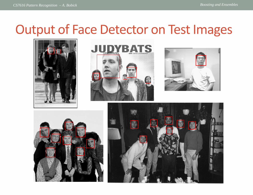
Output of Face Detector on Test Images

Boosting and Ensembles CS7616 Pattern Recognition – A. Bobick
Other detection tasks
Facial Feature Localization
Male vs. female
Profile Detection

Boosting and Ensembles CS7616 Pattern Recognition – A. Bobick
Profile Detection

Boosting and Ensembles CS7616 Pattern Recognition – A. Bobick
Profile Features

Boosting and Ensembles CS7616 Pattern Recognition – A. Bobick
Beyond AdaBoost…

Boosting and Ensembles CS7616 Pattern Recognition – A. Bobick
Why AdaBoost Works: (1) Minimizing a loss function

Boosting and Ensembles CS7616 Pattern Recognition – A. Bobick
(2) Forward stage additive model

Boosting and Ensembles CS7616 Pattern Recognition – A. Bobick
(3) Exponential Loss

Boosting and Ensembles CS7616 Pattern Recognition – A. Bobick
Training error of final classifier is bounded by:
Convex upper bound
Where
exp loss If boosting can make upper bound → 0, then training error → 0
0/1 loss
1
(3) Exponential loss an upper bound on classification error
70 0

Boosting and Ensembles CS7616 Pattern Recognition – A. Bobick
Why Boosting Works? (Cont’d)
Source http://www.stat.ucl.ac.be/

Boosting and Ensembles CS7616 Pattern Recognition – A. Bobick
Loss Function • In Hastie: “easy to show”:
• So AdaBoost is estimating one-half the “log odds” that Pr 𝑌𝑌 = 1 𝑥𝑥 . So doing classification if greater than zero makes sense. Above also implies:

Boosting and Ensembles CS7616 Pattern Recognition – A. Bobick
A better loss function: • A different loss function can be derived from a different
assumed form of probability (logit function in f):
• Minimized by the same f(x) but not the same function.
Binomial deviance

Boosting and Ensembles CS7616 Pattern Recognition – A. Bobick
More on Loss Functions and Classification
• 𝑦𝑦 ⋅ 𝑓𝑓 𝑥𝑥 is called the Margin • The classification rule implies that observations with
positive margin 𝑦𝑦𝑖𝑖𝑓𝑓(𝑥𝑥𝑖𝑖) > 0 were classified correctly, but the negative margin ones are incorrect
• The decision boundary is given by the f(X)=0 • The loss criterion should penalize the negative
margins more heavily than the positive ones. • But how much more…
Boosting and Ensembles CS7616 Pattern Recognition – A. Bobick
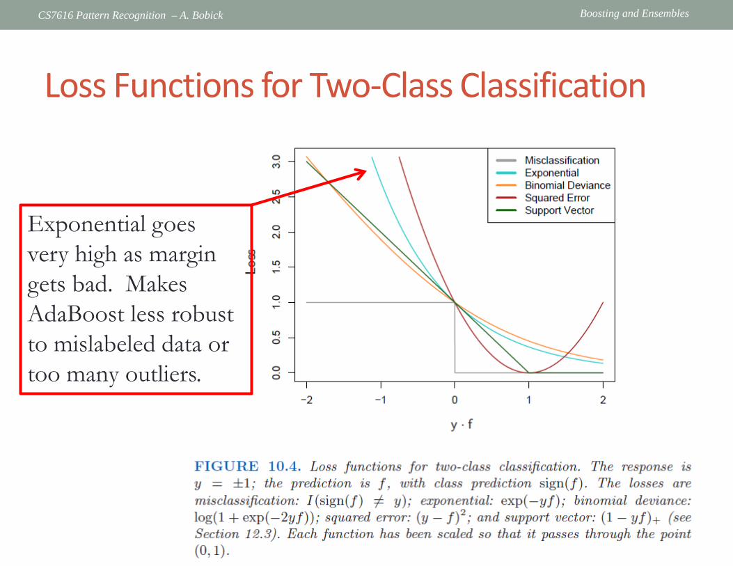
Loss Functions for Two-Class Classification
Exponential goes very high as margin gets bad. Makes AdaBoost less robust to mislabeled data or too many outliers.

Boosting and Ensembles CS7616 Pattern Recognition – A. Bobick
How to “fix” boosting? • AdaBoost analytically minimizes exponential loss.
• Clean equations • Good performance in good cases.
• But, exponential loss sensitive to outliers, misclassified points. • The “binomial deviance” loss function is better behaved. • We should be able to boost any weak learner – like trees. • Can we boost trees for “binomial deviance”?
• Not analytically • But we can numerically – “gradient boosting”
• And can be improved by other tricks: • Stochastic sampling of training points at each stage • Regularization or diminishing effects of each stage

Boosting and Ensembles CS7616 Pattern Recognition – A. Bobick
Loss Function (Cont’d)
Source http://www.stat.ucl.ac.be/

Boosting and Ensembles CS7616 Pattern Recognition – A. Bobick
Trees Reviewed (in Hastie notation) • Trees partition the feature vector (joint
predictor values) into disjoint regions 𝑅𝑅𝑗𝑗 , 𝑗𝑗 = 1, . . , 𝐽𝐽 represented by the terminal nodes
• A constant 𝛾𝛾𝑗𝑗 is assigned to each region, whether regression or classification • The predictive/classification rule 𝑥𝑥∈𝑅𝑅𝑗𝑗𝑓𝑓 𝑥𝑥 = 𝛾𝛾𝑗𝑗
• The tree is: 𝑇𝑇 𝑥𝑥;Θ = ∑ 𝛾𝛾𝑗𝑗𝐼𝐼(𝑥𝑥 ∈𝑅𝑅𝑗𝑗) 𝑗𝑗 where Θ are the parameters of the splits 𝑅𝑅𝑗𝑗 and the values 𝛾𝛾𝑗𝑗
• We want to minimize the loss:
1arg min ( ,ˆ )
i j
J
i jj x R
L y γΘ
= ∈∑Θ = ∑

Boosting and Ensembles CS7616 Pattern Recognition – A. Bobick
Boosting Trees • Finding 𝛾𝛾𝑗𝑗 given 𝑅𝑅𝑗𝑗: this is easy • Finding 𝑅𝑅𝑗𝑗: this is difficult, we typically approximate. We
described the greedy top-down recursive partitioning algorithm
• A boosted tree, is sum of such trees,
Where at each stage m we minimize the :

Boosting and Ensembles CS7616 Pattern Recognition – A. Bobick
Boosting Trees (cont’d) • Given the regions 𝑅𝑅𝑗𝑗,𝑚𝑚 the correct 𝛾𝛾𝑗𝑗,𝑚𝑚 is whatever minimizes
the loss function:
• For exponential loss, if we restrict our trees to be weak learners outputing {−1, +1} then this is exactly AdaBoost and train the same way.
• But if we want a different loss function, need numerical method.

Boosting and Ensembles CS7616 Pattern Recognition – A. Bobick
• Loss function in using prediction f(x) for y is
• The goal is to minimize L(f) w.r.t f, where f is the sum of the trees. But ignore the sum of tree constraint for now. Just think about minimization.
where the parameters f are the values of the approximating function 𝑓𝑓(𝑥𝑥𝑖𝑖) at each of the N data points 𝑥𝑥𝑖𝑖: 𝑓𝑓 = 𝑓𝑓 𝑥𝑥1 , … ,𝑓𝑓 𝑥𝑥𝑁𝑁 .
• Numerical optimization successively approximates 𝒇𝒇� by steps
• Solve it as a sum of component vectors, where 𝑓𝑓0 = ℎ0 is the initial guess and each successive 𝑓𝑓𝑚𝑚 is induced based on the current parameter vector 𝑓𝑓𝑚𝑚−1.
Numerical Optimization
1( ) ( , ( ))
N
i ii
L f L y f x=
= ∑
1,
MN
M m mm
f h h=
= ∈ℜ∑

Boosting and Ensembles CS7616 Pattern Recognition – A. Bobick
1. Choose ℎ𝑚𝑚 = −ρ𝑚𝑚𝑠𝑠𝑚𝑚, where ρ𝑚𝑚 is a scalar and 𝑠𝑠𝑚𝑚 is the gradient of L(f) evaluated at 𝑓𝑓 = 𝑓𝑓𝑚𝑚−1
2. The step length ρm is the (line search) solution to
ρ𝑚𝑚 = arg min𝜌𝜌𝐿𝐿(𝑓𝑓𝑚𝑚−1 − 𝜌𝜌𝑠𝑠𝑚𝑚)
3. The current solution is then updated:
𝑓𝑓𝑚𝑚 = 𝑓𝑓𝑚𝑚−1 − ρ𝑚𝑚𝑠𝑠𝑚𝑚
Steepest Descent

Boosting and Ensembles CS7616 Pattern Recognition – A. Bobick
Gradient Boosting • Forward stagewise boosting is also a very greedy algorithm • The tree predictions can be thought about like negative
gradients • The only difficulty is that the tree components are not
arbitrary
• They are constrained to be the predictions of a 𝐽𝐽𝑚𝑚-terminal node decision tree, whereas the negative gradient is unconstrained steepest descent
• Unfortunately, the gradient is only defined at the training data points and is not applicable to generalizing 𝑓𝑓𝑚𝑚 𝑥𝑥 to new data

Boosting and Ensembles CS7616 Pattern Recognition – A. Bobick
Gradient boosting (cont) • For classification:
• where
• We’re going to approximate gradient by finding a decision tree that’s as close as possible to the gradient.

Boosting and Ensembles CS7616 Pattern Recognition – A. Bobick
Gradient boosting

Boosting and Ensembles CS7616 Pattern Recognition – A. Bobick
Gradient boosting results

Boosting and Ensembles CS7616 Pattern Recognition – A. Bobick
More tweaks • If we fit the “best” tree possible, it will yield a tree
that is deep, as if it were the last tree of the boosting ensemble. • Large trees permit interaction between elements. • Prevent by either penalizing based upon tree size or, believe it
or not, let J=6. • There is the question of how many stages. If go too
far can overfit (worse than Adaboost?) • Need “shrinkage” – from ML:
where 0 < 𝑣𝑣 < 1 . Text actually describes v=.01

Boosting and Ensembles CS7616 Pattern Recognition – A. Bobick

Boosting and Ensembles CS7616 Pattern Recognition – A. Bobick
Interpretation • Single decision trees are often very interpretable • Linear combination of trees loses this important feature • We often learn the relative importance or contribution of
each input variable in predicting the response • Define a measure of relevance for each predictor 𝑋𝑋𝑙𝑙, sum over
the J-1 internal nodes of the tree

Boosting and Ensembles CS7616 Pattern Recognition – A. Bobick
• Relevance of a predictor 𝑋𝑋𝑙𝑙in a single tree (where v(t) is the feature selected):
where 𝚤𝚤�̂�𝑡2is measure of improvement after tree is split is applied to the node. • In a boosted tree the squared relevance:
• Since relative, make the max 100.
Interpretation (Cont’d)

Boosting and Ensembles CS7616 Pattern Recognition – A. Bobick
Relevance

Boosting and Ensembles CS7616 Pattern Recognition – A. Bobick
Illustration (California Housing)

Boosting and Ensembles CS7616 Pattern Recognition – A. Bobick
• Combine weak classifiers to obtain very strong classifier – Weak classifier – slightly better than random on training data – Resulting very strong classifier – can eventually provide zero
training error and
• AdaBoost algorithm • Boosting v. Logistic Regression
– Similar loss functions – LR is single optimization v. Incrementally improving classification
in Boosting
• Boosting is very popular for applications: – Boosted decision stumps – easy to build training system – Very simple to implement and efficient
Boosting Summary