csc 411: lecture 09: naive bayesfidler/teaching/2015/slides/csc411/09_naive_bayes.pdf · today...

$: CSC 411: Lecture 09: Naive Bayesfidler/teaching/2015/slides/CSC411/09_naive_bayes.pdf · Today Classi cation { Multi-dimensional (Gaussian) Bayes classi er Estimate probability densities$
CSC 411: Lecture 09: Naive Bayes

Class based on Raquel Urtasun & Rich Zemel’s lectures

Sanja Fidler

University of Toronto

Feb 8, 2015

Urtasun, Zemel, Fidler (UofT) CSC 411: 09-Naive Bayes Feb 8, 2015 1 / 28

Today

Classification – Multi-dimensional (Gaussian) Bayes classifier

Estimate probability densities from data

Naive Bayes classifier


Generative vs Discriminative

Two approaches to classification:

Discriminative classifiers estimate parameters of decision boundary/classseparator directly from labeled examples

I learn p(y |x) directly (logistic regression models)I learn mappings from inputs to classes (least-squares, neural nets)

Generative approach: model the distribution of inputs characteristic of theclass (Bayes classifier)

I Build a model of p(x|y)I Apply Bayes Rule


Bayes Classifier

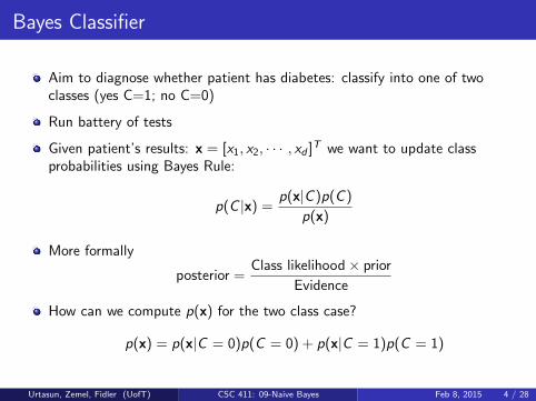
Aim to diagnose whether patient has diabetes: classify into one of twoclasses (yes C=1; no C=0)

Run battery of tests

Given patient’s results: x = [x1, x2, · · · , xd ]T we want to update classprobabilities using Bayes Rule:

p(C |x) =p(x|C )p(C )

p(x)

More formally

posterior =Class likelihood× prior

Evidence

How can we compute p(x) for the two class case?

p(x) = p(x|C = 0)p(C = 0) + p(x|C = 1)p(C = 1)


Classification: Diabetes Example

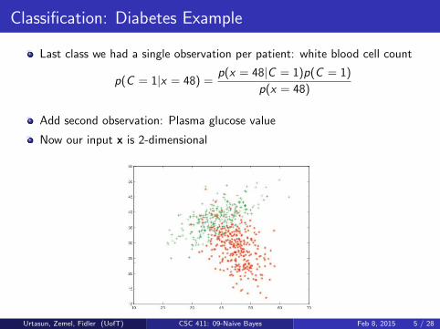
Last class we had a single observation per patient: white blood cell count

p(C = 1|x = 48) =p(x = 48|C = 1)p(C = 1)

p(x = 48)

Add second observation: Plasma glucose value

Now our input x is 2-dimensional


Gaussian Discriminant Analysis (Gaussian Bayes Classifier)

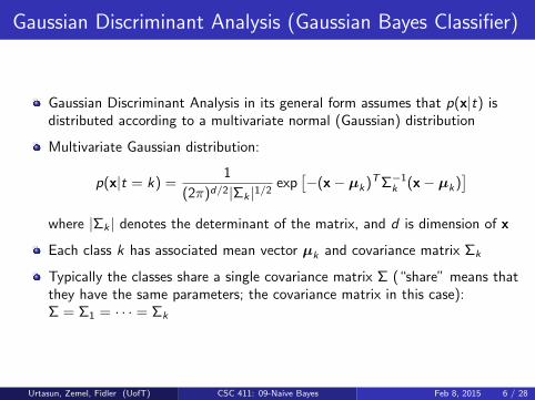
Gaussian Discriminant Analysis in its general form assumes that p(x|t) isdistributed according to a multivariate normal (Gaussian) distribution

Multivariate Gaussian distribution:

p(x|t = k) =1

(2π)d/2|Σk |1/2exp

[−(x− µk)TΣ−1

k (x− µk)]

where |Σk | denotes the determinant of the matrix, and d is dimension of x

Each class k has associated mean vector µk and covariance matrix Σk

Typically the classes share a single covariance matrix Σ (“share” means thatthey have the same parameters; the covariance matrix in this case):Σ = Σ1 = · · · = Σk


Multivariate Data

Multiple measurements (sensors)

d inputs/features/attributes

N instances/observations/examples

X =

x(1)1 x

(1)2 · · · x

(1)d

x(2)1 x

(2)2 · · · x

(2)d

......

. . ....

x(N)1 x

(N)2 · · · x

(N)d


Multivariate Parameters

MeanE[x] = [µ1, · · · , µd ]T

Covariance

Σ = Cov(x) = E[(x− µ)T (x− µ)] =

σ21 σ12 · · · σ1d

σ12 σ22 · · · σ2d

......

. . ....

σd1 σd2 · · · σ2d

Correlation = Corr(x) is the covariance divided by the product of standarddeviation

ρij =σijσiσj


Multivariate Gaussian Distribution

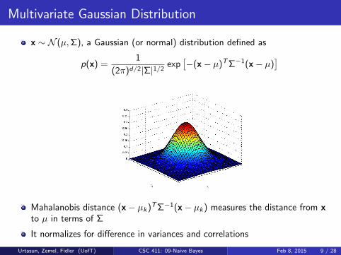
x ∼ N (µ,Σ), a Gaussian (or normal) distribution defined as

p(x) =1

(2π)d/2|Σ|1/2exp

[−(x− µ)TΣ−1(x− µ)

]

Mahalanobis distance (x− µk)TΣ−1(x− µk) measures the distance from xto µ in terms of Σ

It normalizes for difference in variances and correlations


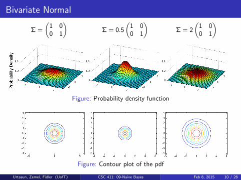
Bivariate Normal

Σ =

(1 00 1

)Σ = 0.5

(1 00 1

)Σ = 2

(1 00 1

)

Figure: Probability density function

Figure: Contour plot of the pdf


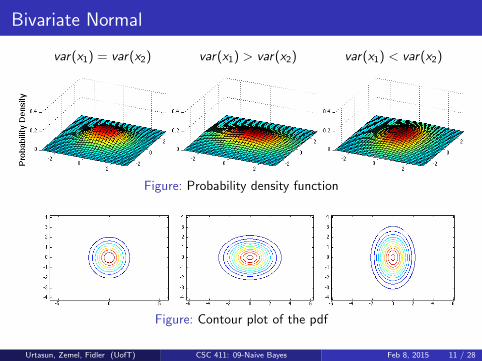
Bivariate Normal

var(x1) = var(x2) var(x1) > var(x2) var(x1) < var(x2)




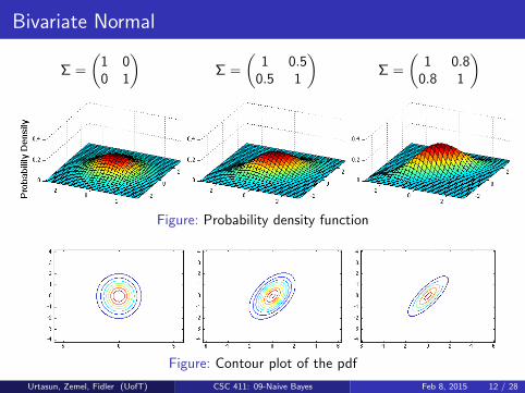
Bivariate Normal

Σ =

(1 00 1

)Σ =

(1 0.5

0.5 1

)Σ =

(1 0.8

0.8 1

)




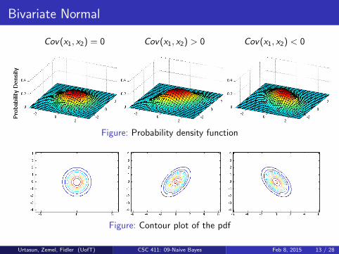
Bivariate Normal

Cov(x1, x2) = 0 Cov(x1, x2) > 0 Cov(x1, x2) < 0




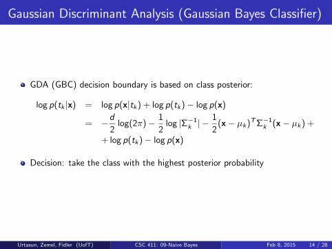
Gaussian Discriminant Analysis (Gaussian Bayes Classifier)

GDA (GBC) decision boundary is based on class posterior:

log p(tk |x) = log p(x|tk) + log p(tk)− log p(x)

= −d

2log(2π)− 1

2log |Σ−1

k | −1

2(x− µk)TΣ−1

k (x− µk) +

+ log p(tk)− log p(x)

Decision: take the class with the highest posterior probability


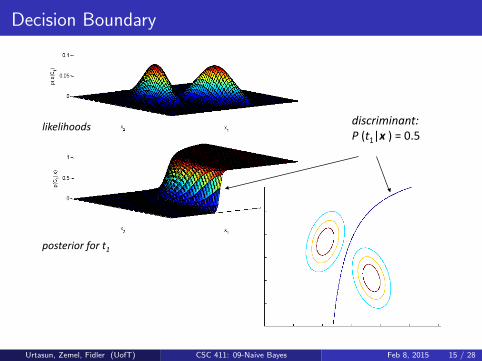
Decision Boundary

likelihoods)

posterior)for)t1)

discriminant:!!P!(t1|x")!=!0.5!


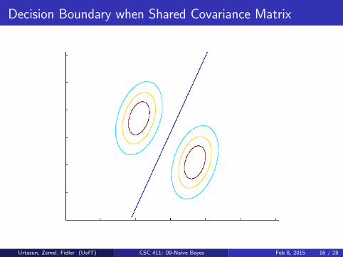
Decision Boundary when Shared Covariance Matrix


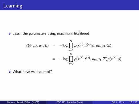
Learning

Learn the parameters using maximum likelihood

`(φ, µ0, µ1,Σ) = − logN∏

n=1

p(x(n), t(n)|φ, µ0, µ1,Σ)

= − logN∏

n=1

p(x(n)|t(n), µ0, µ1,Σ)p(t(n)|φ)

What have we assumed?


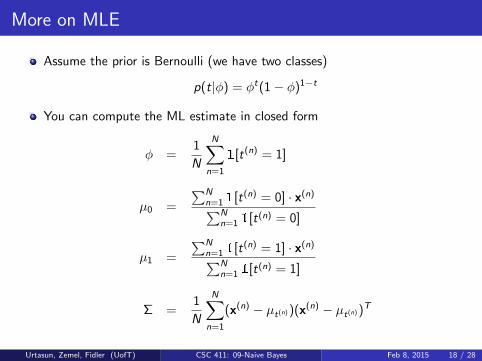
More on MLE

Assume the prior is Bernoulli (we have two classes)

p(t|φ) = φt(1− φ)1−t

You can compute the ML estimate in closed form

φ =1

N

N∑n=1

1[t(n) = 1]

µ0 =

∑Nn=1 1[t(n) = 0] · x(n)∑N

n=1 1[t(n) = 0]

µ1 =

∑Nn=1 1[t(n) = 1] · x(n)∑N

n=1 1[t(n) = 1]

Σ =1

N

N∑n=1

(x(n) − µt(n))(x(n) − µt(n))T


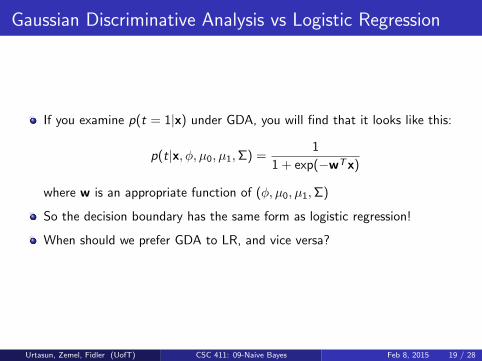
Gaussian Discriminative Analysis vs Logistic Regression

If you examine p(t = 1|x) under GDA, you will find that it looks like this:

p(t|x, φ, µ0, µ1,Σ) =1

1 + exp(−wTx)

where w is an appropriate function of (φ, µ0, µ1,Σ)

So the decision boundary has the same form as logistic regression!

When should we prefer GDA to LR, and vice versa?


Gaussian Discriminative Analysis vs Logistic Regression

GDA makes stronger modeling assumption: assumes class-conditional data ismultivariate Gaussian

If this is true, GDA is asymptotically efficient (best model in limit of large N)

But LR is more robust, less sensitive to incorrect modeling assumptions

Many class-conditional distributions lead to logistic classifier

When these distributions are non-Gaussian, in limit of large N, LR beatsGDA


Simplifying the Model

What if x is high-dimensional?

For Gaussian Bayes Classifier, if input x is high-dimensional, then covariancematrix has many parameters

Save some parameters by using a shared covariance for the classes

Any other idea you can think of?


Naive Bayes

Naive Bayes is an alternative generative model: Assumes featuresindependent given the class

p(x|t = k) =d∏

i=1

p(xi |t = k)

Assuming likelihoods are Gaussian, how many parameters required for NaiveBayes classifier?

Important note: Naive Bayes does not assume a particular distribution


Naive Bayes Classifier

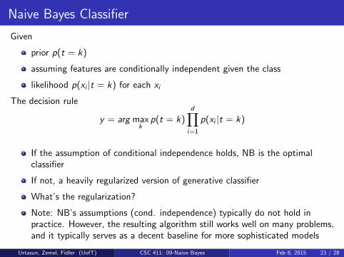
Given

prior p(t = k)

assuming features are conditionally independent given the class

likelihood p(xi |t = k) for each xi

The decision rule

y = arg maxk

p(t = k)d∏

i=1

p(xi |t = k)

If the assumption of conditional independence holds, NB is the optimalclassifier

If not, a heavily regularized version of generative classifier

What’s the regularization?

Note: NB’s assumptions (cond. independence) typically do not hold inpractice. However, the resulting algorithm still works well on many problems,and it typically serves as a decent baseline for more sophisticated models


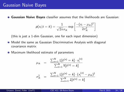
Gaussian Naive Bayes

Gaussian Naive Bayes classifier assumes that the likelihoods are Gaussian:

p(xi |t = k) =1√

2πσikexp

[−(xi − µik)2

2σ2ik

](this is just a 1-dim Gaussian, one for each input dimension)

Model the same as Gaussian Discriminative Analysis with diagonalcovariance matrix

Maximum likelihood estimate of parameters

µik =

∑Nn=1 1[t(n) = k] · x (n)i∑N

n=1 1[t(n) = k]

σ2ik =

∑Nn=1 1[t(n) = k] · (x (n)i − µik)2∑N

n=1 1[t(n) = k]


Decision Boundary: Shared Variances (between Classes)

variances may be different


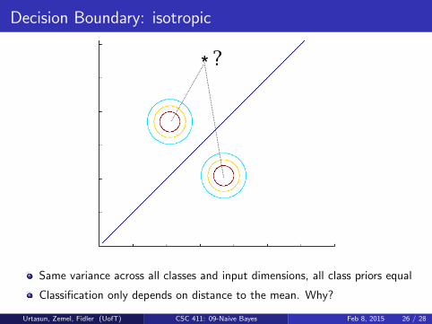
Decision Boundary: isotropic

* ?

Same variance across all classes and input dimensions, all class priors equal

Classification only depends on distance to the mean. Why?


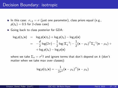
Decision Boundary: isotropic

In this case: σi,k = σ (just one parameter), class priors equal (e.g.,p(tk) = 0.5 for 2-class case)

Going back to class posterior for GDA:

log p(tk |x) = log p(x|tk) + log p(tk)− log p(x)

= −d

2log(2π)− 1

2log |Σ−1

k | −1

2(x− µk)TΣ−1

k (x− µk) +

+ log p(tk)− log p(x)

where we take Σk = σ2I and ignore terms that don’t depend on k (don’tmatter when we take max over classes):

log p(tk |x) = − 1

2σ2(x− µk)T (x− µk)


Spam Classification

You have examples of emails that are spam and non-spam

How would you classify spam vs non-spam?

Think about it at home, solution in the next tutorial


csc 411: lecture 09: naive bayesfidler/teaching/2015/slides/csc411/09_naive_bayes.pdf · today...

Documents