csc311: data structures 1 chapter 13: graphs ii objectives: graph adt: operations graph...

CSC311: Data StructuresCSC311: Data Structures 11

Chapter 13: Graphs IIChapter 13: Graphs II

Objectives:Objectives:

Graph ADT: OperationsGraph ADT: Operations Graph Implementation: Data structuresGraph Implementation: Data structures Graph Traversals: DFS and BFSGraph Traversals: DFS and BFS Directed graphsDirected graphs Weighted graphsWeighted graphs Shortest pathsShortest paths Minimum Spanning Trees (MST)Minimum Spanning Trees (MST)

Graphs IIGraphs II CSC311: Data StructuresCSC311: Data Structures 22

Weighted GraphsWeighted GraphsIn a weighted graph, each edge has an associated In a weighted graph, each edge has an associated numerical value, called the weight of the edgenumerical value, called the weight of the edgeEdge weights may represent distances, costs, etc.Edge weights may represent distances, costs, etc.Example:Example:– In a flight route graph, the weight of an edge represents the In a flight route graph, the weight of an edge represents the

distance in miles between the endpoint airportsdistance in miles between the endpoint airports

ORD PVD

MIADFW

SFO

LAX

LGA

HNL

849

802

13871743

1843

10991120

1233

337

2555

142

12

05


Shortest Paths Shortest Paths Given a weighted graph and two vertices Given a weighted graph and two vertices uu and and vv, we want , we want to find a path of minimum total weight between to find a path of minimum total weight between uu and and v.v.– Length of a path is the sum of the weights of its edges.Length of a path is the sum of the weights of its edges.

Example:Example:– Shortest path between Providence and HonoluluShortest path between Providence and Honolulu

ApplicationsApplications– Internet packet routing Internet packet routing – Flight reservationsFlight reservations– Driving directionsDriving directions

ORD PVD

MIADFW

SFO

LAX

LGA

HNL

849

802

13871743

1843

10991120

1233337

2555

142

12

05


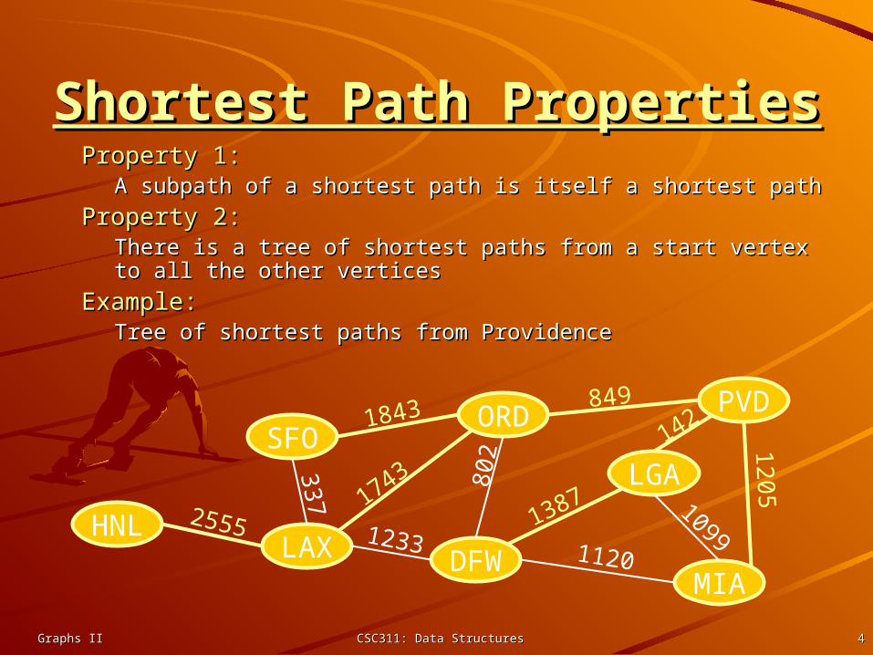
Shortest Path PropertiesShortest Path PropertiesProperty 1:Property 1:

A subpath of a shortest path is itself a shortest pathA subpath of a shortest path is itself a shortest path

Property 2:Property 2:There is a tree of shortest paths from a start vertex to all the There is a tree of shortest paths from a start vertex to all the other verticesother vertices

Example:Example:Tree of shortest paths from ProvidenceTree of shortest paths from Providence

ORD PVD

MIADFW

SFO

LAX

LGA

HNL

849

802

13871743

1843

10991120

1233337

2555

142

12

05


Dijkstra’s AlgorithmDijkstra’s Algorithm

The distance of a vertex The distance of a vertex vv from a vertex from a vertex ss is the is the length of a shortest path length of a shortest path between between ss and and vv

Dijkstra’s algorithm Dijkstra’s algorithm computes the distances computes the distances of all the vertices from a of all the vertices from a given start vertex given start vertex ss

Assumptions:Assumptions:– the graph is connectedthe graph is connected– the edges are undirectedthe edges are undirected– the edge weights are the edge weights are

nonnegativenonnegative

We grow a “We grow a “cloudcloud” of ” of vertices, beginning with vertices, beginning with ss and and eventually covering all the eventually covering all the verticesvertices

We store with each vertex We store with each vertex vv a a label label dd((vv)) representing the representing the distance of distance of vv from from ss in the in the subgraph consisting of the subgraph consisting of the cloud and its adjacent cloud and its adjacent verticesvertices

At each stepAt each step– We add to the cloud the We add to the cloud the

vertex vertex u u outside the cloud outside the cloud with the smallest distance with the smallest distance label, label, dd((uu))

– We update the labels of the We update the labels of the vertices adjacent to vertices adjacent to uu


Edge RelaxationEdge Relaxation

Consider an edge Consider an edge e e ((u,zu,z)) such thatsuch that– uu is the vertex most is the vertex most

recently added to the recently added to the cloudcloud

– zz is not in the cloud is not in the cloud

The relaxation of edge The relaxation of edge e e updates distance updates distance dd((zz) ) as as follows:follows:

dd((zz)) min{min{dd((zz)),d,d((uu) ) weightweight((ee)})}

d(z) 75

d(u) 5010

zsu

d(z) 60

d(u) 5010

zsu

e

e


ExampleExample

CB

A

E

D

F

0

428

48

7 1

2 5

2

3 9

CB

A

E

D

F

0

328

5 11

48

7 1

2 5

2

3 9

CB

A

E

D

F

0

328

5 8

48

7 1

2 5

2

3 9

CB

A

E

D

F

0

327

5 8

48

7 1

2 5

2

3 9


Example (cont.)Example (cont.)

CB

A

E

D

F

0

327

5 8

48

7 1

2 5

2

3 9

CB

A

E

D

F

0

327

5 8

48

7 1

2 5

2

3 9


Dijkstra’s AlgorithmDijkstra’s Algorithm

A priority queue stores A priority queue stores the vertices outside the the vertices outside the cloudcloud– Key: distanceKey: distance– Element: vertexElement: vertex

Locator-based methodsLocator-based methods– insertinsert((k,ek,e) ) returns a returns a

locator locator – replaceKeyreplaceKey((l,kl,k)) changes changes

the key of an itemthe key of an item

We store two labels with We store two labels with each vertex:each vertex:– Distance (d(v) label)Distance (d(v) label)– locator in priority locator in priority

queuequeue

Algorithm DijkstraDistances(G, s)Q new heap-based priority queuefor all v G.vertices()

if v ssetDistance(v, 0)

else setDistance(v, )

l Q.insert(getDistance(v), v)setLocator(v,l)

while Q.isEmpty()u Q.removeMin() for all e G.incidentEdges(u)

{ relax edge e }z G.opposite(u,e)r getDistance(u) weight(e)if r getDistance(z)

setDistance(z,r) Q.replaceKey(getLocator(z),r)


Analysis of Dijkstra’s AlgorithmAnalysis of Dijkstra’s AlgorithmGraph operationsGraph operations– Method incidentEdges is called once for each vertexMethod incidentEdges is called once for each vertex

Label operationsLabel operations– We set/get the distance and locator labels of vertex We set/get the distance and locator labels of vertex zz OO(deg((deg(zz))))

timestimes– Setting/getting a label takes Setting/getting a label takes OO(1)(1) time time

Priority queue operationsPriority queue operations– Each vertex is inserted once into and removed once from the Each vertex is inserted once into and removed once from the

priority queue, where each insertion or removal takes priority queue, where each insertion or removal takes OO(log (log nn) ) timetime

– The key of a vertex in the priority queue is modified at most The key of a vertex in the priority queue is modified at most deg(deg(ww) ) times, where each key change takes times, where each key change takes OO(log (log nn) ) time time

Dijkstra’s algorithm runs in Dijkstra’s algorithm runs in OO((((n n m m) log ) log nn)) time provided the time provided the graph is represented by the adjacency list structuregraph is represented by the adjacency list structure– Recall that Recall that v v deg(deg(vv)) 22mm

The running time can also be expressed as The running time can also be expressed as OO((mm log log nn)) since since the graph is connectedthe graph is connected


Shortest Paths TreeShortest Paths TreeUsing the template Using the template method pattern, we method pattern, we can extend Dijkstra’s can extend Dijkstra’s algorithm to return a algorithm to return a tree of shortest paths tree of shortest paths from the start vertex from the start vertex to all other verticesto all other verticesWe store with each We store with each vertex a third label:vertex a third label:– parent edge in the parent edge in the

shortest path treeshortest path tree

In the edge relaxation In the edge relaxation step, we update the step, we update the parent labelparent label

Algorithm DijkstraShortestPathsTree(G, s)

…

for all v G.vertices()…

setParent(v, )…

for all e G.incidentEdges(u){ relax edge e }z G.opposite(u,e)r getDistance(u) weight(e)if r getDistance(z)

setDistance(z,r)setParent(z,e) Q.replaceKey(getLocator(z),r)


Why Dijkstra’s Algorithm WorksWhy Dijkstra’s Algorithm WorksDijkstra’s algorithm is based on the greedy Dijkstra’s algorithm is based on the greedy method. It adds vertices by increasing distance.method. It adds vertices by increasing distance.

CB

A

E

D

F

0

327

5 8

48

7 1

2 5

2

3 9

Suppose it didn’t find all shortest distances. Let F be the first wrong vertex the algorithm processed.

When the previous node, D, on the true shortest path was considered, its distance was correct.

But the edge (D,F) was relaxed at that time!

Thus, so long as d(F)>d(D), F’s distance cannot be wrong. That is, there is no wrong vertex.


Why It Doesn’t Work for Why It Doesn’t Work for Negative-Weight EdgesNegative-Weight Edges

– If a node with a negative If a node with a negative incident edge were to be incident edge were to be added late to the cloud, it added late to the cloud, it could mess up distances for could mess up distances for vertices already in the vertices already in the cloud. cloud.

CB

A

E

D

F

0

457

5 9

48

7 1

2 5

6

0 -8

Dijkstra’s algorithm is based on the greedy method. It adds vertices by increasing distance.

C’s true distance is 1, but it is already in the

cloud with d(C)=5!


Bellman-Ford AlgorithmBellman-Ford AlgorithmWorks even with Works even with negative-weight edgesnegative-weight edgesMust assume directed Must assume directed edges (for otherwise we edges (for otherwise we would have negative-would have negative-weight cycles)weight cycles)Iteration i finds all Iteration i finds all shortest paths that use i shortest paths that use i edges.edges.Running time: O(nm).Running time: O(nm).Can be extended to Can be extended to detect a negative-weight detect a negative-weight cycle if it exists cycle if it exists – How?How?

Algorithm BellmanFord(G, s)for all v G.vertices()



for i 1 to n-1 dofor each e G.edges()

{ relax edge e }u G.origin(e)z G.opposite(u,e)r getDistance(u) weight(e)if r getDistance(z)

setDistance(z,r)


-2

Bellman-Ford ExampleBellman-Ford Example

0

48

7 1

-2 5

-2

3 9

0

48

7 1

-2 53 9

Nodes are labeled with their d(v) values

-2

-28

0

4

48

7 1

-2 53 9

8 -2 4

-15

61

9

-25

0

1

-1

9

48

7 1

-2 5

-2

3 94


DAG-based AlgorithmDAG-based AlgorithmWorks even with Works even with negative-weight negative-weight edgesedgesUses topological Uses topological orderorderDoesn’t use any Doesn’t use any fancy data structuresfancy data structuresIs much faster than Is much faster than Dijkstra’s algorithmDijkstra’s algorithmRunning time: Running time: O(n+m).O(n+m).

Algorithm DagDistances(G, s)for all v G.vertices()



Perform a topological sort of the verticesfor u 1 to n do {in topological order}

for each e G.outEdges(u){ relax edge e }z G.opposite(u,e)r getDistance(u) weight(e)if r getDistance(z)

setDistance(z,r)


-2

DAG ExampleDAG Example

0

48

7 1

-5 5

-2

3 9

0

48

7 1

-5 53 9

Nodes are labeled with their d(v) values

-2

-28

0

4

48

7 1

-5 53 9

-2 4

-1

1 7

-25

0

1

-1

7

48

7 1

-5 5

-2

3 94

1

2 43

6 5

1

2 43

6 5

8

1

2 43

6 5

1

2 43

6 5

5

0

(two steps)


Minimum Spanning TreesMinimum Spanning TreesSpanning subgraphSpanning subgraph

– Subgraph of a graph Subgraph of a graph GG containing all the vertices containing all the vertices of of GG

Spanning treeSpanning tree– Spanning subgraph that is Spanning subgraph that is

itself a (free) treeitself a (free) tree

Minimum spanning tree (MST)Minimum spanning tree (MST)– Spanning tree of a Spanning tree of a

weighted graph with weighted graph with minimum total edge minimum total edge weightweight

ApplicationsApplications– Communications networksCommunications networks– Transportation networksTransportation networks

ORD

PIT

ATL

STL

DEN

DFW

DCA

101

9

8

6

3

25

7

4


Cycle PropertyCycle PropertyCycle Property:Cycle Property:

– Let Let TT be a minimum be a minimum spanning tree of a spanning tree of a weighted graph weighted graph GG

– Let Let ee be an edge of be an edge of GG that is not in that is not in T T and and CC let be the cycle let be the cycle formed by formed by ee with with TT

– For every edge For every edge ff of of C,C, weightweight((ff)) weightweight((ee))

Proof:Proof:– By contradictionBy contradiction– If If weightweight((ff)) weightweight((ee) ) we we

can get a spanning can get a spanning tree of smaller weight tree of smaller weight by replacing by replacing ee with with ff

84

2 36

7

7

9

8e

C

f

84

2 36

7

7

9

8

C

e

f

Replacing f with e yieldsa better spanning tree


U V

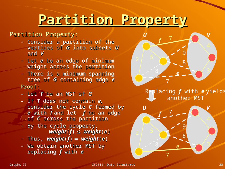
Partition PropertyPartition PropertyPartition Property:Partition Property:

– Consider a partition of the vertices Consider a partition of the vertices of of GG into subsets into subsets UU and and VV

– Let Let ee be an edge of minimum be an edge of minimum weight across the partitionweight across the partition

– There is a minimum spanning tree There is a minimum spanning tree of of GG containing edge containing edge ee

Proof:Proof:– Let Let TT be an MST of be an MST of GG– If If TT does not contain does not contain e,e, consider consider

the cycle the cycle CC formed by formed by ee with with T T and and let let ff be an edge of be an edge of CC across the across the partitionpartition

– By the cycle property,By the cycle property,weightweight((ff)) weightweight((ee))

– Thus, Thus, weightweight((ff)) weightweight((ee))– We obtain another MST by We obtain another MST by

replacing replacing f f with with ee

74

2 85

7

3

9

8 e

f

74

2 85

7

3

9

8 e

f

Replacing f with e yieldsanother MST

U V


Kruskal’s AlgorithmKruskal’s AlgorithmA priority queue stores the edges outside the cloud

Key: weight Element: edge

At the end of the algorithm

We are left with one cloud that encompasses the MST

A tree T which is our MST

Algorithm KruskalMST(G)for each vertex V in G do

define a Cloud(v) of {v}let Q be a priority queue.Insert all edges into Q using their

weights as the keyT while T has fewer than n-1 edges do

edge e = T.removeMin()Let u, v be the endpoints of eif Cloud(v) Cloud(u) then

Add edge e to TMerge Cloud(v) and Cloud(u)

return T


Data Structure for Kruskal AlgortihmData Structure for Kruskal AlgortihmThe algorithm maintains a The algorithm maintains a forest of treesforest of treesAn edge is accepted it if An edge is accepted it if connects distinct treesconnects distinct treesWe need a data structure We need a data structure that maintains a that maintains a partitionpartition, i.e., a collection , i.e., a collection of disjoint sets, with the of disjoint sets, with the operations:operations:

--findfind(u): return the set (u): return the set storing ustoring u

--unionunion(u,v): replace the (u,v): replace the sets storing u and v with sets storing u and v with their uniontheir union


Representation of Representation of a Partitiona Partition

Each set is stored in a sequenceEach set is stored in a sequence

Each element has a reference back to the setEach element has a reference back to the set– operationoperation find find(u) takes O(1) time, and returns the set (u) takes O(1) time, and returns the set

of which u is a member.of which u is a member.– in operation in operation unionunion(u,v), we move the elements of the (u,v), we move the elements of the

smaller set to the sequence of the larger set and smaller set to the sequence of the larger set and update their referencesupdate their references

– the time for operation the time for operation unionunion(u,v) is min(n(u,v) is min(nuu,n,nvv), where ), where nnuu and n and nvv are the sizes of the sets storing u and v are the sizes of the sets storing u and v

Whenever an element is processed, it goes into Whenever an element is processed, it goes into a set of size at least double, hence each a set of size at least double, hence each element is processed at most log n timeselement is processed at most log n times


Partition-Based ImplementationPartition-Based ImplementationA partition-based version of Kruskal’s Algorithm A partition-based version of Kruskal’s Algorithm performs cloud merges as unions and tests as performs cloud merges as unions and tests as finds.finds.

Algorithm Kruskal(G):

Input: A weighted graph G.

Output: An MST T for G.

Let P be a partition of the vertices of G, where each vertex forms a separate set.

Let Q be a priority queue storing the edges of G, sorted by their weights

Let T be an initially-empty tree

while Q is not empty do

(u,v) Q.removeMinElement()

if P.find(u) != P.find(v) then

Add (u,v) to T

P.union(u,v)

return T

Running time: O((n+m)log n)


Kruskal Kruskal ExampleExample

JFK

BOS

MIA

ORD

LAXDFW

SFO BWI

PVD

8672704

187

1258

849

144740

1391

184

946

1090

1121

2342

1846 621

802

1464

1235

337


JFK

BOS

MIA

ORD

LAXDFW

SFO BWI

PVD

8672704

187

1258

849

144740

1391

184

946

1090

1121

2342

1846 621

802

1464

1235

337

ExampleExample


ExampleExample

JFK

BOS

MIA

ORD

LAXDFW

SFO BWI

PVD

8672704

187

1258

849

144740

1391

184

946

1090

1121

2342

1846 621

802

1464

1235

337


Prim-Jarnik’s AlgorithmPrim-Jarnik’s AlgorithmSimilar to Dijkstra’s algorithm (for a connected Similar to Dijkstra’s algorithm (for a connected graph)graph)We pick an arbitrary vertex We pick an arbitrary vertex ss and we grow the and we grow the MST as a cloud of vertices, starting from MST as a cloud of vertices, starting from ssWe store with each vertex We store with each vertex vv a label a label dd((vv)) = the = the smallest weight of an edge connecting smallest weight of an edge connecting v v to a to a vertex in the cloud vertex in the cloud

At each step: We add to the cloud the vertex u outside the cloud with the smallest distance label We update the labels of the vertices adjacent to u


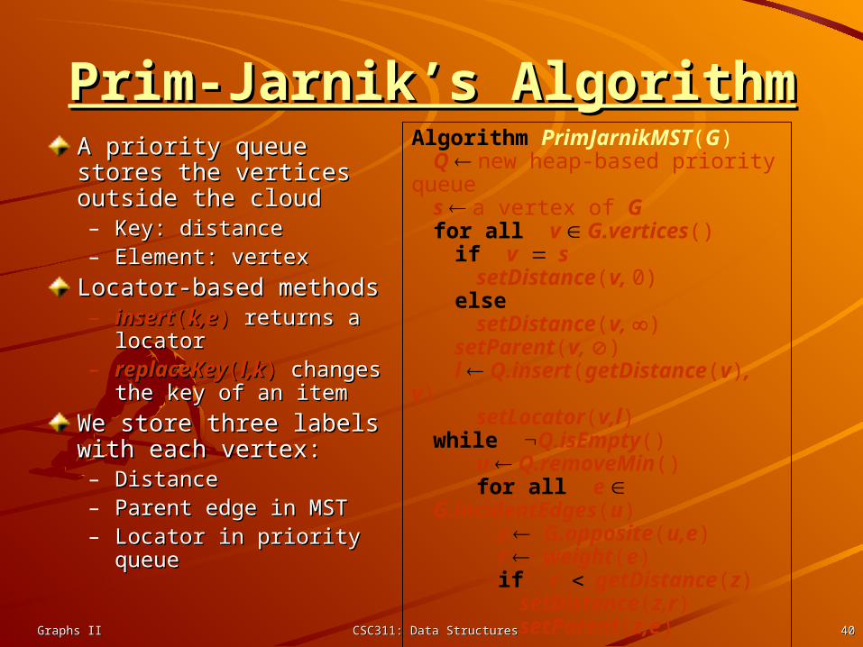
Prim-Jarnik’s AlgorithmPrim-Jarnik’s AlgorithmA priority queue stores A priority queue stores the vertices outside the the vertices outside the cloudcloud– Key: distanceKey: distance– Element: vertexElement: vertex

Locator-based methodsLocator-based methods– insertinsert((k,ek,e) ) returns a returns a

locator locator – replaceKeyreplaceKey((l,kl,k)) changes changes

the key of an itemthe key of an item

We store three labels We store three labels with each vertex:with each vertex:– DistanceDistance– Parent edge in MSTParent edge in MST– Locator in priority queueLocator in priority queue

Algorithm PrimJarnikMST(G)Q new heap-based priority queues a vertex of Gfor all v G.vertices()



setParent(v, )l Q.insert(getDistance(v), v)

setLocator(v,l)while Q.isEmpty()

u Q.removeMin() for all e G.incidentEdges(u)

z G.opposite(u,e)r weight(e)if r getDistance(z)

setDistance(z,r)setParent(z,e)

Q.replaceKey(getLocator(z),r)


ExampleExample

BD

C

A

F

E

74

28

5

7

3

9

8

07

2

8

BD

C

A

F

E

74

28

5

7

3

9

8

07

2

5

7

BD

C

A

F

E

74

28

5

7

3

9

8

07

2

5

7

BD

C

A

F

E

74

28

5

7

3

9

8

07

2

5 4

7


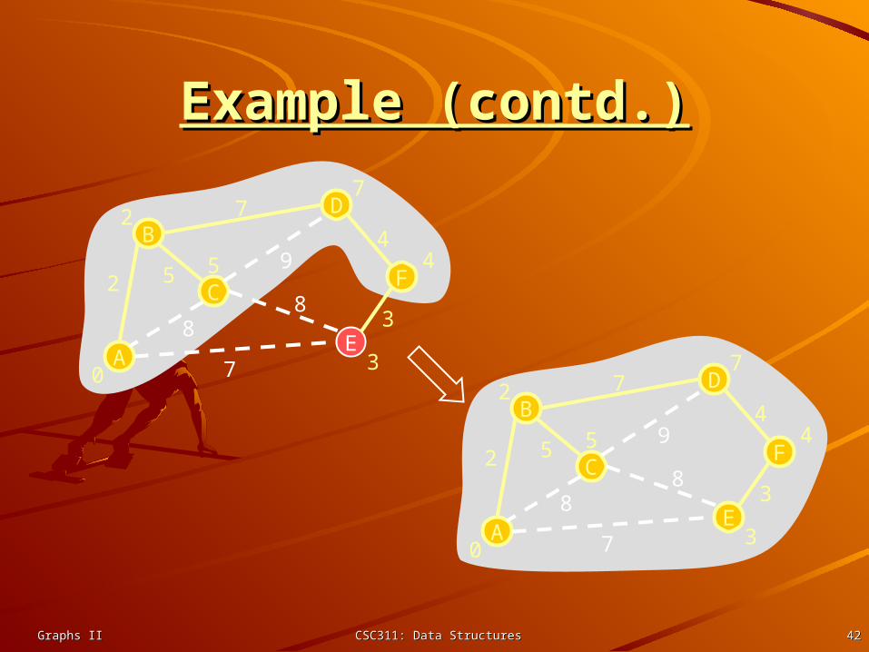
Example (contd.)Example (contd.)

BD

C

A

F

E

74

28

5

7

3

9

8

03

2

5 4

7

BD

C

A

F

E

74

28

5

7

3

9

8

03

2

5 4

7


AnalysisAnalysisGraph operationsGraph operations– Method incidentEdges is called once for each vertexMethod incidentEdges is called once for each vertex

Label operationsLabel operations– We set/get the distance, parent and locator labels of vertex We set/get the distance, parent and locator labels of vertex zz

OO(deg((deg(zz)))) times times– Setting/getting a label takes Setting/getting a label takes OO(1)(1) time time

Priority queue operationsPriority queue operations– Each vertex is inserted once into and removed once from the Each vertex is inserted once into and removed once from the

priority queue, where each insertion or removal takes priority queue, where each insertion or removal takes OO(log (log nn) ) timetime

– The key of a vertex The key of a vertex ww in the priority queue is modified at most in the priority queue is modified at most deg(deg(ww) ) times, where each key change takes times, where each key change takes OO(log (log nn) ) time time

Prim-Jarnik’s algorithm runs in Prim-Jarnik’s algorithm runs in OO((((n n m m) log ) log nn)) time provided time provided the graph is represented by the adjacency list structurethe graph is represented by the adjacency list structure– Recall that Recall that v v deg(deg(vv)) 22mm

The running time is The running time is OO((mm log log nn)) since the graph is connected since the graph is connected

csc311: data structures 1 chapter 13: graphs ii objectives: graph adt: operations graph...

Documents