csc373 - approximation algorithms · csc373 - approximation algorithms vincent maccio vincent...

CSC373 - Approximation Algorithms

Vincent Maccio

Vincent MaccioCSC373 - Approximation Algorithms 1 / 22

Algorithm Classification

The following is all informal.

• Problems can be broken down and classified into different groupsbased on how hard they are to solve

• Most problems we’ve seen in this course and most you’ve seenpreviously are easy problems

• Let P be the set of problems which can be solved in polynomial time,that is if for some k a problem has an algorithm which solves it inO(nk) then that problem is in P

• sorting a list, shortest path in a graph, determining primes, etc. are allin P

• If for a problem one can be given a solution and determine if thatsolution is correct or not in polynomial time, then that problem is saidto be in NP


Algorithm Classification - cont

• For example, determining if there exists a solution to a Knapsackproblem which gives you value V is hard to do, but to determine if agiven set of items is a solution or not which gives a value of at leastV is easy

• Just sum up the values to see if it’s greater than V and sum up theweights to see if it’s less than the capacity

• A problem is said to be NP-complete if it is the hardest problem tosolve in NP (if you can solve any NP-complete problem you can solveall NP problems)

• A problem is said to be NP-hard if it’s at least as hard asNP-complete problems


Algorithm Classification - Observations

See if these make sense to you from the previous definitions

• P ⊆ NP

• There exist problems which are NP-hard, but not NP

• (NP-hard - NP-complete) ∪P = ∅• P ∩ NP-complete =?


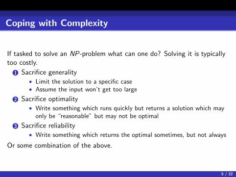
Coping with Complexity

If tasked to solve an NP-problem what can one do? Solving it is typicallytoo costly.

1 Sacrifice generality• Limit the solution to a specific case• Assume the input won’t get too large

2 Sacrifice optimality• Write something which runs quickly but returns a solution which may

only be “reasonable” but may not be optimal

3 Sacrifice reliability• Write something which returns the optimal sometimes, but not always

Or some combination of the above.


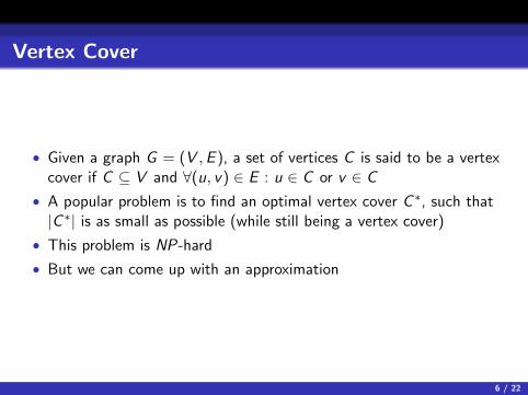
Vertex Cover

• Given a graph G = (V ,E ), a set of vertices C is said to be a vertexcover if C ⊆ V and ∀(u, v) ∈ E : u ∈ C or v ∈ C

• A popular problem is to find an optimal vertex cover C ∗, such that|C ∗| is as small as possible (while still being a vertex cover)

• This problem is NP-hard

• But we can come up with an approximation


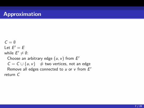
Approximation

C = ∅Let E ′ = Ewhile E ′ 6= ∅:

Choose an arbitrary edge (u, v) from E ′

C = C ∪ {u, v} # two vertices, not an edgeRemove all edges connected to u or v from E ′

return C


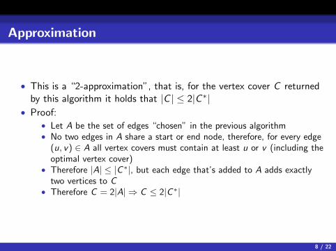
Approximation

• This is a “2-approximation”, that is, for the vertex cover C returnedby this algorithm it holds that |C | ≤ 2|C ∗|

• Proof:• Let A be the set of edges “chosen” in the previous algorithm• No two edges in A share a start or end node, therefore, for every edge

(u, v) ∈ A all vertex covers must contain at least u or v (including theoptimal vertex cover)

• Therefore |A| ≤ |C∗|, but each edge that’s added to A adds exactlytwo vertices to C

• Therefore C = 2|A| ⇒ C ≤ 2|C∗|


The Travelling Salesman Problem

• Given a graph G = (V ,E ) and a start node a ∈ V find a path in Gwhich visits each vertex other than a exactly once, and which startsat a and ends at a

• Such a path is called a tour of G

• The length of a tour is the sum of all the edge weights on said tour

• In the travelling salesman problem, the goal is to find the shortesttour possible

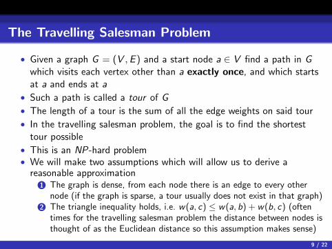
• This is an NP-hard problem• We will make two assumptions which will allow us to derive a

reasonable approximation1 The graph is dense, from each node there is an edge to every other

node (if the graph is sparse, a tour usually does not exist in that graph)2 The triangle inequality holds, i.e. w(a, c) ≤ w(a, b) + w(b, c) (often

times for the travelling salesman problem the distance between nodes isthought of as the Euclidean distance so this assumption makes sense)


TSP Approximation

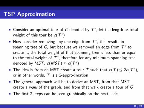
• Consider an optimal tour of G denoted by T ∗, let the length or totalweight of this tour be c(T ∗)

• Now consider removing any one edge from T ∗, this results inspanning tree of G , but because we removed an edge from T ∗ tocreate it, the total weight of that spanning tree is less than or equalto the total weight of T ∗, therefore for any minimum spanning treedenoted by MST , c(MST ) ≤ c(T ∗)

• The idea is from an MST create a tour T such that c(T ) ≤ 2c(T ∗),or in other words, T is a 2-approximation

• The general approach will be to derive an MST, from that MSTcreate a walk of the graph, and from that walk create a tour of G

• The first 2 steps can be seen graphically on the next slide


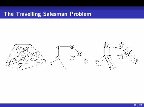
The Travelling Salesman Problem


TSP Approximation

• A walk is a sequence of vertices of the graph such that each vertexappears at least once in the walk (it also starts and ends at a)

• A walk of an MST can be defined recursively where one simply calls“walk” on each child node of a given vertex

• Informally one can note that while a vertex may be visited anarbitrary number of times (1+ how many children it has), each edgeof the MST is travelled across exactly twice (see the previous slide toconvince yourself)

• Therefore, letting W denote a walk of an MST and letting the totalweight or length of that walk be denoted by c(W ), it is known thatc(W ) = 2c(MST )


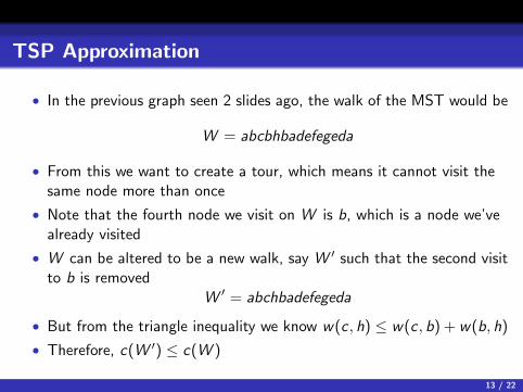
TSP Approximation

• In the previous graph seen 2 slides ago, the walk of the MST would be

W = abcbhbadefegeda

• From this we want to create a tour, which means it cannot visit thesame node more than once

• Note that the fourth node we visit on W is b, which is a node we’vealready visited

• W can be altered to be a new walk, say W ′ such that the second visitto b is removed

W ′ = abchbadefegeda

• But from the triangle inequality we know w(c , h) ≤ w(c, b) + w(b, h)

• Therefore, c(W ′) ≤ c(W )


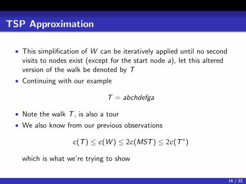
TSP Approximation

• This simplification of W can be iteratively applied until no secondvisits to nodes exist (except for the start node a), let this alteredversion of the walk be denoted by T

• Continuing with our example

T = abchdefga

• Note the walk T , is also a tour

• We also know from our previous observations

c(T ) ≤ c(W ) ≤ 2c(MST ) ≤ 2c(T ∗)

which is what we’re trying to show


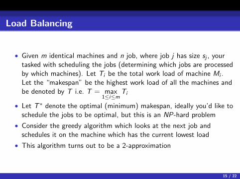
Load Balancing

• Given m identical machines and n job, where job j has size sj , yourtasked with scheduling the jobs (determining which jobs are processedby which machines). Let Ti be the total work load of machine Mi .Let the “makespan” be the highest work load of all the machines andbe denoted by T i.e. T = max

1≤i≤mTi

• Let T ∗ denote the optimal (minimum) makespan, ideally you’d like toschedule the jobs to be optimal, but this is an NP-hard problem

• Consider the greedy algorithm which looks at the next job andschedules it on the machine which has the current lowest load

• This algorithm turns out to be a 2-approximation


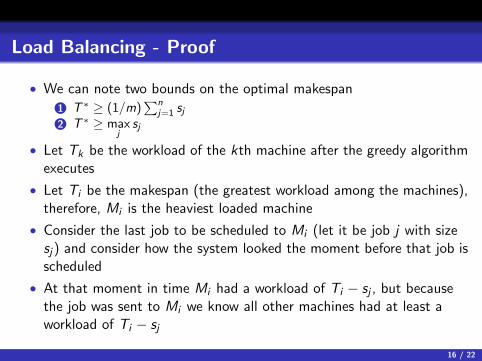
Load Balancing - Proof

• We can note two bounds on the optimal makespan

1 T ∗ ≥ (1/m)∑n

j=1 sj2 T ∗ ≥ max

jsj

• Let Tk be the workload of the kth machine after the greedy algorithmexecutes

• Let Ti be the makespan (the greatest workload among the machines),therefore, Mi is the heaviest loaded machine

• Consider the last job to be scheduled to Mi (let it be job j with sizesj) and consider how the system looked the moment before that job isscheduled

• At that moment in time Mi had a workload of Ti − sj , but becausethe job was sent to Mi we know all other machines had at least aworkload of Ti − sj


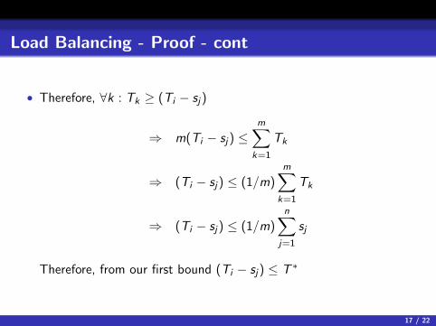
Load Balancing - Proof - cont

• Therefore, ∀k : Tk ≥ (Ti − sj)

⇒ m(Ti − sj) ≤m∑

k=1

Tk

⇒ (Ti − sj) ≤ (1/m)m∑

k=1

Tk

⇒ (Ti − sj) ≤ (1/m)n∑

j=1

sj

Therefore, from our first bound (Ti − sj) ≤ T ∗


Load Balancing - Proof - cont

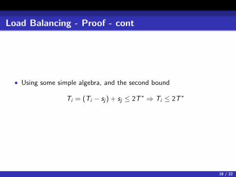
• Using some simple algebra, and the second bound

Ti = (Ti − sj) + sj ≤ 2T ∗ ⇒ Ti ≤ 2T ∗


Knapsack Approximation

• Recall the greedy algorithm which orders the items by v/w and keepsselecting the best item that fits until no items are left

• It turns out this algorithm is arbitrarily bad, but it can be fixed with aquick hack

• Consider the following algorithm:


Knapsack Approximation

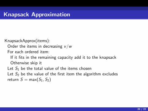
KnapsackApprox(items):Order the items in decreasing v/wFor each ordered item:

If it fits in the remaining capacity add it to the knapsackOtherwise skip it

Let S1 be the total value of the items chosenLet S2 be the value of the first item the algorithm excludesreturn S = max(S1, S2)


Knapsack Approximation - Proof

• Let k be the index such that the kth item is the first not to fit in theknapsack (following the greedy algorithm)

• Consider the solution of including the first k − 1 items and then afraction of the kth item which fills the Knapsack, giving appropriatefractional value

• Let this fractional solution have total value SF

• This fractional solution has at least as large a value as the optimalsolution to the non-fractional knapsack problem (think about it)

• Therefore SF ≥ S∗


Knapsack Approximation - Proof - cont

• SF =∑k−1

i=1 vi + fvk , where 0 ≤ f ≤ 1

• From the algorithm S1 ≥∑k−1

i=1 vi and S2 ≥ fvk

• Therefore SF ≤ S1 + S2 ≤ 2S

• From the previous slide S∗ ≤ SF , so S∗ ≤ 2S


csc373 - approximation algorithms · csc373 - approximation algorithms vincent maccio vincent...

Documents