csce 411h design and analysis of algorithms set 4: transform and conquer prof. evdokia nikolova*...
TRANSCRIPT

CSCE 411HDesign and Analysis
of Algorithms
Set 4: Transform and ConquerProf. Evdokia Nikolova*
Spring 2013
CSCE 411H, Spring 2013: Set 4 1
* Slides adapted from Prof. Jennifer Welch

General Idea of Transform & Conquer1. Transform the original problem
instance into a different problem instance
2. Solve the new instance3. Transform the solution of the new
instance into the solution for the original instance
CSCE 411H, Spring 2013: Set 4 2

Varieties of Transform & Conquer[Levitin]
Transform to a simpler or more convenient instance of the same problem
“instance simplification Transform to a different representation of
the same instance “representation change”
Transform to an instance of a different problem with a known solution
“problem reduction”
CSCE 411H, Spring 2013: Set 4 3

Instance Simplification: Presorting Sort the input data first This simplifies several problems:
checking whether a particular element in an array is unique
computing the median and mode (value that occurs most often) of an array of numbers
searching for a particular element once array is sorted, we can use the decrease &
conquer binary search algorithm used in several convex hull algorithms
CSCE 411H, Spring 2013: Set 4 4

Instance Simplification: Solving System of Equations A system of n linear equations in n
unknowns: a11x1 + a12x2 + … + a1nxn = b1
… an1x1 + an2x2 + … + annxn = bn
Cast as a matrix problem: Ax = b, where A is n x n matrix, x and b are n-
vectors To solve for all the x’s, solve Ax = b for x
CSCE 411H, Spring 2013: Set 4 5

Motivation for Solving Systems of Linear Equations http://aix1.uottawa.ca/~jkhoury/syste
m.html geometry networks heat distribution chemistry economics linear programming games
CSCE 411H, Spring 2013: Set 4 6

Solving System of Equations One way to solve Ax = b for x:
compute A−1
multiply both sides by A−1
A−1Ax = A−1b x = A−1b
Drawback is that computing matrix inverses suffers from numerical instability in practice
Try another approach…
CSCE 411H, Spring 2013: Set 4 7

LUP Decomposition If A is triangular, solving Ax = b for x is easy and fast
using successive substitutions (how fast?) Transform this problem into one involving only triangular
matrices instance simplification!
Find n x n matrix L with all 1’s on diagonal and all 0’s above the
diagonal (“unit lower-triangular”) n x n matrix U with all 0’s below the diagonal (“upper-triangular”) n x n matrix P of 0’s and 1’s with exactly one 1 in each row and
each column (“permutation matrix”)
such that PA = LU
CSCE 411H, Spring 2013: Set 4 8

Using LUP Decomposition We want to solve Ax = b. Assume we have L, U and P with desired properties so that PA = LU Multiply both sides of Ax = b by P to obtain PAx = Pb
Since P is a permutation matrix, Pb is easy to compute and is just a reordering of the vector b, call it b’
Substitute LU for PA to obtain LUx = b’ Let y be the vector (as of yet unknown) that equals Ux;
rewrite as Ly = b’ although U is known, x is not yet known
Solve Ly = b’ for y since L is triangular, this is easy
Now that y is known, solve y = Ux for x since U is triangular, this is easy
CSCE 411H, Spring 2013: Set 4 9

Solving Ax = b with LUP Decomp. Assuming the L, U, and P are given,
pseudocode is on p. 817 of [CLRS] Running time is Θ(n2) Example: <board>
Calculating L, U and P is more involved and takes Θ(n3) time. (See [CLRS].)
CSCE 411H, Spring 2013: Set 4 10
Instance Simplification: Balanced Binary Search Trees Transform an unbalanced binary search
tree into a balanced binary search tree Benefit is guaranteed O(log n) time for
searching, inserting and deleting as opposed to possibility of Θ(n) time
Examples: AVL trees red-black trees splay trees
CSCE 411H, Spring 2013: Set 4 11

Representation Change: Balanced Search Trees Convert a basic binary search tree into a
search tree that is more than binary: a node can have more than two children a node can store more than one data item
Can get improved performance (w.r.t. constant factors)
Examples: 2-3 trees B-trees
CSCE 411H, Spring 2013: Set 4 12

B-Trees: Motivation Designed for very large data sets that cannot all
fit in main memory at a time Instead, data is stored on disk Fact 1: Disk access is orders of magnitude
slower than main memory access Typically a disk access is needed for each node
encountered during operations on a search tree For a balanced binary search tree, this would be about
c log2 n, where c is a small constant and n is number of items
CSCE 411H, Spring 2013: Set 4 13

B-Trees: Motivation Can we reduce the time? Even if not asymptotically, what about reducing the
constants? Constants do matter
Reduce the height by having a bushier tree have more than two children at each node store more than two keys in each node
Fact 2: Each disk access returns a fixed amount of information (a page). Size is determined by hardware and operating system Typically 512 to 4096 bytes
Let size of tree node be page size
CSCE 411H, Spring 2013: Set 4 14

B-Tree Applications Keeping index information for large
amounts of data stored on disk databases file systems
CSCE 411H, Spring 2013: Set 4 15

B-Tree Definition B-tree with minimum degree t is a rooted tree such that
1. each node has between t−1 and 2t−1 keys, in increasing order (root can have fewer keys)
2. each non-leaf node has one more child than it has keys
3. all keys in a node’s i-th subtree lie between the node’s (i−1)st key and its i-th key
4. all leaves have the same depth Points 1-3 are generalization of binary search trees to
larger branching factor Point 4 controls the height
CSCE 411H, Spring 2013: Set 4 16

B-Tree Example
B-tree with minimum degree 21. each node has between 1 and 3 keys, in sorted order2. each non-leaf node has 2 to 4 children, one more than
number of keys3. keys are in proper subtrees4. all leaves have depth 1
CSCE 411H, Spring 2013: Set 4 17
26 41
13 17 28 30 31 45 50
B-Tree Height Theorem: Any n-key B-tree with minimum
degree t has height h ≤ logt((n+1)/2). Height is still O(log n) but logarithm base is t
instead of 2 savings in constant factor of log2t, which is
substantial since t is generally very large Remember: log2x = (log2t)*(logtx)
Proof: Calculate minimum number of keys in a B-tree of height h and solve for h.
CSCE 411H, Spring 2013: Set 4 18

Searching in a B-Tree Straightforward generalization of
searching in a binary search tree to search for k, start at root:
1. find largest i such that k ≤ i-th key in current node
2. if k = ith key then return “found”3. else if current node is a leaf then return
“not found”4. else recurse on root of i-th subtree
CSCE 411H, Spring 2013: Set 4 19

Running Time of B-Tree Search CPU time:
Line 1 takes O(t) (or O(log2 t) if using binary search)
Number of recursive calls is O(height) = O(logt n) Total is O(t logt n)
Number of disk accesses: each recursive call requires at most one disk
access, to get the next node O(logt n) (the height)
CSCE 411H, Spring 2013: Set 4 20

B-Tree Insert To insert a new key, need to
obey bounds on branching factor / maximum number of keys per node
keep all leaves at the same depth
Do some examples on a B-tree with minimum degree 2 each node has 1, 2, or 3 keys each node has 2, 3, or 4 children
CSCE 411H, Spring 2013: Set 4 21

B-Tree Insert Examples
CSCE 411H, Spring 2013: Set 4 22
F T
A D H L Q U Z
F T
C D H L Q U ZA
insert C
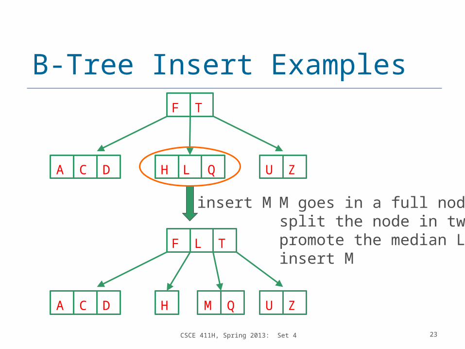
B-Tree Insert Examples
CSCE 411H, Spring 2013: Set 4 23
F T
C D H L Q U ZA
insert M
F L
C D H M Q U ZA
T
M goes in a full node;split the node in two;promote the median L;insert M
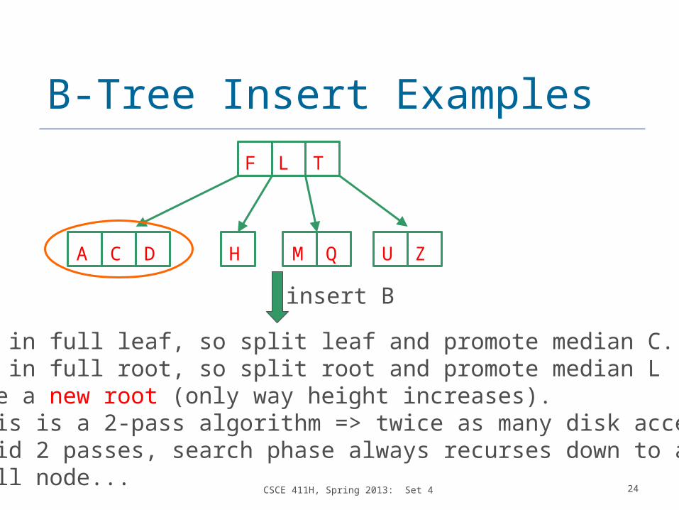
B-Tree Insert Examples
CSCE 411H, Spring 2013: Set 4 24
insert B
F L
C D H M Q U ZA
T
B goes in full leaf, so split leaf and promote median C.C goes in full root, so split root and promote median Lto make a new root (only way height increases).But this is a 2-pass algorithm => twice as many disk accesses.To avoid 2 passes, search phase always recurses down to a non-full node...

B-Tree Insert with One Pass
CSCE 411H, Spring 2013: Set 4 25
F L
C D H M Q U ZA
T
To insert B, start at root to find proper place; proactivelysplit root since it is full
F
L
C D H M Q U ZA
T

B-Tree Insert with One Pass
CSCE 411H, Spring 2013: Set 4 26
Recurse to node containing F; since not full no need to split.
F
L
C D H M Q U ZA
T
Recurse to left-most leaf, where B belongs. Since it is full, split it, promote the median C to the parent, and insert B.

B-Tree Insert with One Pass
CSCE 411H, Spring 2013: Set 4 27
Final result of inserting B.
L
FC
D H M Q U Z
T
BA

Splitting a B-Tree Node split(x,i,y) input:
non-full node x full node y which is i-th child of x
result: split y into two equal size nodes with t−1
nodes each insert the median key of the old y into x
CSCE 411H, Spring 2013: Set 4 28

Splitting a B-Tree Node
CSCE 411H, Spring 2013: Set 4 29
x:
< 2t−1 keys
2t−1 keysα m βy:
i... ...x:
≤ 2t−1 keys
t−1 keys
α βy:
i... ...
m
t−1 keys
i+1

B-Tree Insert Algorithm (Input:T, k) if root r is full, i.e. has (2t−1) keys then
allocate a new node s make s the new root make r the first child of s split(s,1,r) insert-non-full(s,k)
else insert-non-full(r,k)
CSCE 411H, Spring 2013: Set 4 30
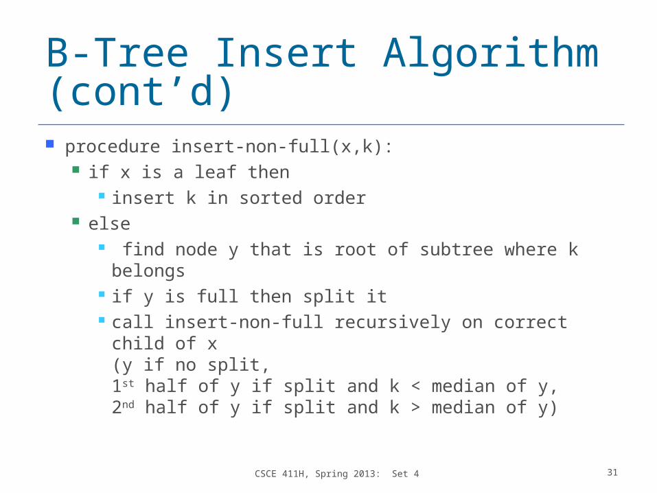
B-Tree Insert Algorithm (cont’d) procedure insert-non-full(x,k):
if x is a leaf then insert k in sorted order
else find node y that is root of subtree where k
belongs if y is full then split it call insert-non-full recursively on correct child of x
(y if no split,1st half of y if split and k < median of y,2nd half of y if split and k > median of y)
CSCE 411H, Spring 2013: Set 4 31
Running Time of B-Tree Insert Same as search:
O(t logt n) CPU time
O(logt n) disk access
Practice: insert F, S, Q, K, C, L, H, T, V, W into a B-tree with minimum degree t = 3
CSCE 411H, Spring 2013: Set 4 32

Deleting from a B-Tree Pitfalls:
Be careful that a node does not end up with too few keys
When deleting from a non-leaf node, need to rearrange the children (remember, number of children must be one greater than the number of keys)
CSCE 411H, Spring 2013: Set 4 33

B-Tree Delete Algorithm
delete(x,k): // called initially with x = root
1. if k is in x and x is a leaf thendelete k from x // we will ensure that x has ≥ t
keys
2. if k is in x and x is not a leaf then
CSCE 411H, Spring 2013: Set 4 34
kx...
y z
.........

B-Tree Delete Algorithm (cont’d)2(a) if y has ≥ t keys then
find k’ = pred(k) // in y’s subtree
delete(y,k’) // recursive call
replace k with k’ in x
CSCE 411H, Spring 2013: Set 4 35
kx
y z
k’
k’x
y z

B-Tree Delete Algorithm (cont’d)2(b) else if z has ≥ t keys then
find k’ = succ(k) // in z’s subtree
delete(z,k’) // recursive call
replace k with k’ in x
CSCE 411H, Spring 2013: Set 4 36
kx
y z
k’
k’x
y z

B-Tree Delete Algorithm (cont’d)2(c) else // both y and z have < t keys
merge y, k, z into a new node w
delete(w,k) // recursive call
CSCE 411H, Spring 2013: Set 4 37
kx
y z
k
x
y z
w

B-Tree Delete Algorithm (cont’d)3. if k is not in (internal) node x then
let y be root of x’s subtree where k belongs3(a) if y has < t keys but has a neighboring sibling z
with ≥ t keys theny borrows a key from z via x // note
moving subtrees
CSCE 411H, Spring 2013: Set 4 38
25 45
10 20 22 30
x
z y
22 45
10 20 25 30
x
yz
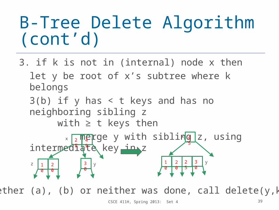
B-Tree Delete Algorithm (cont’d)3. if k is not in (internal) node x then
let y be root of x’s subtree where k belongs3(b) if y has < t keys and has no neighboring sibling z
with ≥ t keys then merge y with sibling z, using
intermediate key in z
CSCE 411H, Spring 2013: Set 4 39
whether (a), (b) or neither was done, call delete(y,k)
25 45
10 20 30
x
z y
45
10 20 25 30
x
y

Behavior of B-Tree Delete As long as k has not yet been found, we continue in a
single downward pass, with no backtracking. If k is found in an internal node, we may have to find
pred or succ of k, call it k’, delete k’ from its old place, and then go back to where k is and replace k with k’.
However, finding and deleting k’ can be done in a single downward pass, since k’ will be in a leaf (basic property of search trees).
O(logt n) disk access
O(t logt n) CPU time
CSCE 411H, Spring 2013: Set 4 40

Problem Reduction: Computing Least Common Multiple lcm(m,n) is the smallest integer that is
divisible by both m and n Ex: lcm(11,5) = 55 and lcm(24,60) = 120
One algorithm for finding lcm: multiply all common factors of m and n, all factors of m not in n, and all factors of n not in m Ex: 24 = 2*2*2*3, 60 = 2*2*3*5,
lcm(24,60) = (2*2*3)*2*5 = 120 But how to find prime factors of m and n?
CSCE 411H, Spring 2013: Set 4 41

Reduce Least Common Multiple to Greatest Common Denominator Try another approach. gcd(m,n) is product of all common factors of m and n So gcd(m,n)*lcm(m,n) includes every factor in both
gcd and lcm twice, every factor in m but not n exactly once, and every factor in n but not m exactly once
Thus gcd(m,n)*lcm(m,n) = m*n. I.e., lcm(m,n) = m*n/gcd(m,n) So if we can solve gcd, we can solve lcm And we can solve gcd with Euclid’s algorithm
CSCE 411H, Spring 2013: Set 4 42

Problem Reduction: Counting Paths in a Graph How many paths are there in this
graph between b and d?
CSCE 411H, Spring 2013: Set 4 43
a b
c d
Counting Paths in a Graph Claim: Adjacency matrix A to the k-
th power gives number of paths of length (exactly) k between all pairs
Reduce problem of counting paths to problem of multiplying matrices!
CSCE 411H, Spring 2013: Set 4 44

Proof of Claim Basis: A1 = A gives all paths of length 1 Induction: Suppose Ak gives all paths of length
k. Show for Ak+1 = AkA. (i,j) entry of Ak+1 is sum, over all vertices h, of
(i,h) entry of Ak times (h,j) entry of A:
CSCE 411H, Spring 2013: Set 4 45
i jh
all paths from i to h with length k
path from h to j with length 1

Computing Number of Paths Maximum length (simple) path is n−1. So we have to compute An−1. Do n−2 matrix multiplications
brute force or Strassen’s O(n4) or O(n3.8…) running time
Or, do successive doubling (A2, A4, A8, A16,…) about log2n multiplications O(n3log n) or O(n2.8…log n) running time
CSCE 411H, Spring 2013: Set 4 46

Problem Reduction Tool: Linear Programming Many problems related to finding an
optimal solution for something can be reduced to an instance of the linear programming problem:
optimize a linear function of several variables subject to constraints each constraint is a linear equation or
linear inequality
CSCE 411H, Spring 2013: Set 4 47

Linear Program Example An organization wants to invest $100 million in stocks,
bonds, and cash. Assume interest rates are:
stocks: 10% bonds: 7% cash: 3%
Institutional restrictions: amount in stock cannot be more than a third of amount in bonds amount in cash must be at least a quarter of the amount in stocks
and bonds How should money manager invest to maximize return?
CSCE 411H, Spring 2013: Set 4 48

Mathematical Formulation of the Example x = amount in stocks (in millions of dollars) y = amount in bonds z = amount in cashmaximize (.10)*x + (.70)*y + (.03)*zsubject to
x+y+z = 100x ≤ y/3z ≥ (x+y)/4x ≥ 0, y ≥ 0, z ≥ 0
CSCE 411H, Spring 2013: Set 4 49
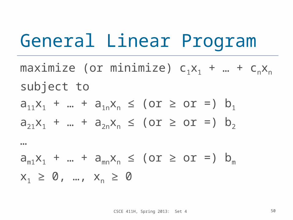
General Linear Programmaximize (or minimize) c1x1 + … + cnxn
subject toa11x1 + … + a1nxn ≤ (or ≥ or =) b1
a21x1 + … + a2nxn ≤ (or ≥ or =) b2
…am1x1 + … + amnxn ≤ (or ≥ or =) bm
x1 ≥ 0, …, xn ≥ 0
CSCE 411H, Spring 2013: Set 4 50

Linear Programs with 2 Variables
maximize x1 + x2
subject to4x1 – x2 ≤ 8
2x1 + x2 ≤ 10
5x1 – 2x2 ≥ –2
x1, x2 ≥ 0
CSCE 411H, Spring 2013: Set 4 51
feasible region
objective function
x1 = 2, x2 = 6is optimal solution
(not drawnto scale)
x1 +x
2 = z4x
1 –
x2 ≤
8
5x1 –
2x 2
≥ –
2
2x1 + x
2 ≤ 10
x1x1 ≥ 0
x2
x 2 ≥
0

Solving a Linear Program Given a linear program, there are 3 possibilities:
the feasible region is empty the feasible region and the optimal value are unbounded the feasible region is bounded and there is an optimal value
Three ways to solve a linear program: simplex method: travel around the feasible region from
corner to corner until finding optimal worst-case exponential time, average case is polynomial time
ellipsoid method: a divide-and-conquer approach polynomial worst-case, but slow in practice
interior point methods polynomial worst-case, reasonable in practice
CSCE 411H, Spring 2013: Set 4 52
most common in practice

Use of Linear Programming Later we will study algorithms to solve
linear programs. Now we’ll give some examples of
converting other problems into linear programs.
CSCE 411H, Spring 2013: Set 4 53

Reducing a Problem to a Linear Program What unknowns are involved?
These will be the variables x1, x2,…
What quantity is to be minimized or maximized? How to express this quantity in terms of the variables? This will be the objective function
What are the constraints on the problem and how to state them w.r.t. the variables? Constraints must be linear
CSCE 411H, Spring 2013: Set 4 54

Reducing a Problem to a Linear Program: Example A tailor can sew pants and shirts. It takes him 2.5 hours to sew a pair of pants and 3.5
hours to sew a shirt. A pair of pants uses 3 yards of fabric and a shirt uses
2 yards of fabric. The tailor has 40 hours available for sewing and has
50 yards of fabric. He makes a profit of $10 per pair of pants and $15
per shirt. How many pants and how many shirts should he sew
to maximize his profit?
CSCE 411H, Spring 2013: Set 4 55

Reducing a Problem to a Linear Program: Example Solution Variables:
x1 = number of pants to sew x2 = number of shirts to sew
Objective function: maximize 10*x1 + 15*x2
Constraints: time: (2.5)*x1 + (3.5)*x2 ≤ 40 fabric: 3*x1 + 2*x2 ≤ 50 nonnegativity: x1 ≥ 0, x2 ≥ 0
CSCE 411H, Spring 2013: Set 4 56

Knapsack Problem as a Linear Program Suppose thief can steal part of an object
“fractional” knapsack problem For each item j, 1 ≤ j ≤ n,
vj is value of (entire) item j wj is weight of (entire) item j xj is fraction of item j that is taken
maximize v1x1 + … + vnxn
subject to w1x1 + … wnxn ≤ W (knapsack limit) 0 ≤ xj ≤ 1, for j = 1,…,n
CSCE 411H, Spring 2013: Set 4 57

A Shortest Path Problem as a Linear Program: Alternative LP What is the shortest path distance from s to
t in weighted directed graph G = (V,E,w)? For each v in V, let dv be a variable
modeling the distance from s to v.maximize dt
subject todv ≤ du + w(u,v) for each (u,v) in E
ds = 0
CSCE 411H, Spring 2013: Set 4 58

A Shortest Path Problem as a Linear Program What is the shortest path distance from s to
t in weighted directed graph G = (V,E,w)? For each e in E, let xe be an indicator
variable modeling whether edge e is in the path.
minimize ∑ we xe
subject to
for all i in Vxe ≥ 0
CSCE 411H, Spring 2013: Set 4 59