cse 5211 analysis of algorithm noteswds/classes/aa/handouts/notes.pdfcse 5211 analysis of algorithm...
TRANSCRIPT
CSE 5211 Analysis of Algorithm NotesWilliam David Shoaff
Spring 2018 (Friday 30th March, 2018)
Preliminaries
• Read and understand the syllabus
• Edward Tufte recommends this structure for presentations:
– Provide audience 1 to 2 pages of notes
– Allow audience 10 to 20 minutes to read notes
– Glare at those who are not reading (his wry sense of humor?)
– While fleshing-out notes ask and answer questions
• I’m going to change Tufte’s formula a bit.
– I’ll provide a few pages of notes before class
– Audience will read the notes before class
– Audience will develop a list of questions
– Audience will bring notes and questions to class
Contents
Preliminaries 1
Personal Assignment 2
Team Assignment 8
Questions and Problems 10
Algorithms 17
Algorithm Design 20
Mathematical Tools 24
More Mathematical Tools 27
Convolutions 29
Representative Problems 33
Binomial Coefficients 37
Divide and Conquer 40
The Quicksort Algorithm 43
Numerical Analysis 59
Amortized Cost Models 64
Greedy Algorithms 67
Dynamic Programming 75
Dynamic Programming, Part 2 82
Graph Algorithms 96
Strongly Connected Components 99
Backtracking Algorithms 101
Complexity 115
Computability 123
cse 5211 analysis of algorithm notes 2
Personal Assignment
One quarter of a student’s course grade is based on personal performance in software development, exper-imentation, and reporting. The basic chores are:
• Write code for a well-known, simple problem. Typically, the code is at most a few dozen lines.
• Test the code on a range of input sizes, collecting and plotting the running times.
• Use the test data to find a function that well approximates the data.
• Analyze the code’s syntax to develop a mathematical model of the algorithm’s time complexity: Anasymptotic analysis.
This term’s personal software development and analysis project is on Gaussian elimination.
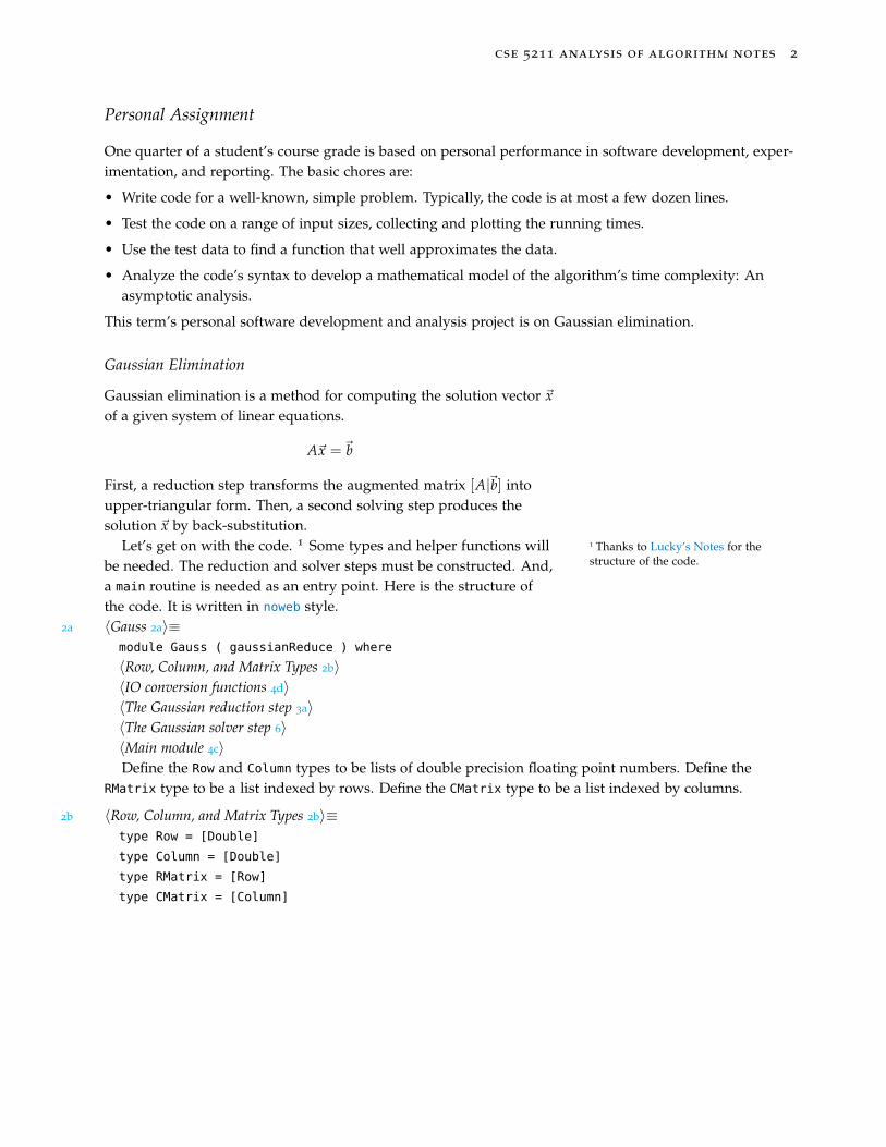
Gaussian Elimination
Gaussian elimination is a method for computing the solution vector ~xof a given system of linear equations.
A~x =~b
First, a reduction step transforms the augmented matrix [A|~b] intoupper-triangular form. Then, a second solving step produces thesolution ~x by back-substitution.
Let’s get on with the code. 1 Some types and helper functions will 1 Thanks to Lucky’s Notes for thestructure of the code.be needed. The reduction and solver steps must be constructed. And,
a main routine is needed as an entry point. Here is the structure ofthe code. It is written in noweb style.
2a 〈Gauss 2a〉≡module Gauss ( gaussianReduce ) where
〈Row, Column, and Matrix Types 2b〉〈IO conversion functions 4d〉〈The Gaussian reduction step 3a〉〈The Gaussian solver step 6〉〈Main module 4c〉Define the Row and Column types to be lists of double precision floating point numbers. Define the
RMatrix type to be a list indexed by rows. Define the CMatrix type to be a list indexed by columns.
2b 〈Row, Column, and Matrix Types 2b〉≡type Row = [Double]
type Column = [Double]
type RMatrix = [Row]
type CMatrix = [Column]

cse 5211 analysis of algorithm notes 3
The Reduction Step
The reduction process used in Gaussian elimination transforms a matrix into upper-triangular form. Pictori-ally, for a small example.
p · · · |·a · · · |·b · · · |·c · · · |·
7→
1 · · · |·0 p · · |·0 · · · |·0 · · · |·
7→
1 · · · |·0 1 · · |·0 0 p · |·0 0 · · |·
7→
1 · · · |·0 1 · · |·0 0 1 · |·0 0 0 1 |·
To reduce a matrix to upper-triangular form repeat these steps iteratively across all rows of the matrix. Forthe first row:
1. Assume p, the pivot, is not 0 and normalize the row by scaling it by 1/p.
2. Repeatedly, multiply the normalized row by a, b, c and subtract the result row from second, third, andfourth rows, respectively.
3a 〈The Gaussian reduction step 3a〉≡gaussianReduce :: RMatrix -> RMatrix
gaussianReduce matrix = foldl reducerow matrix [0..length matrix-1] where
reducerow :: RMatrix -> Int -> RMatrix
reducerow m r = let
〈Pick the row to reduce by, its pivot, and normalize this pivot row 3b〉〈Construct a function that reduces other rows 3c〉〈Apply the reduction function to rows below the pivot 4a〉〈Piece the matrix back together 4b〉
• Pick out the r-th row of matrix m, using !!, Haskell’s indexing operator.
• Pick out the r-th value in the r-th row and call it p, the pivot. To keep things simple, assume these pivotelements along the main diagonal never equal 0.
• Normalize the row by dividing each element in it by the pivot p. The Haskell idiom that does this is tomap the divide by p) function (/ p) across the row. Call the normalized row row’.
3b 〈Pick the row to reduce by, its pivot, and normalize this pivot row 3b〉≡row = m !! r
p = row !! r
row’ = map (/ p) row
Now, to reduce another row, say nrow, by row’ apply the function
nr ∗ a− b (where nr is the r-th element in nrow)
to each entry a in row and b in nrow. The Haskell idiom for this is to zip the function with the values in row’
and nrow.
3c 〈Construct a function that reduces other rows 3c〉≡reduceonerow nrow = let nr = nrow !! r in zipWith (\a b -> nr*a - b) row’ nrow
cse 5211 analysis of algorithm notes 4
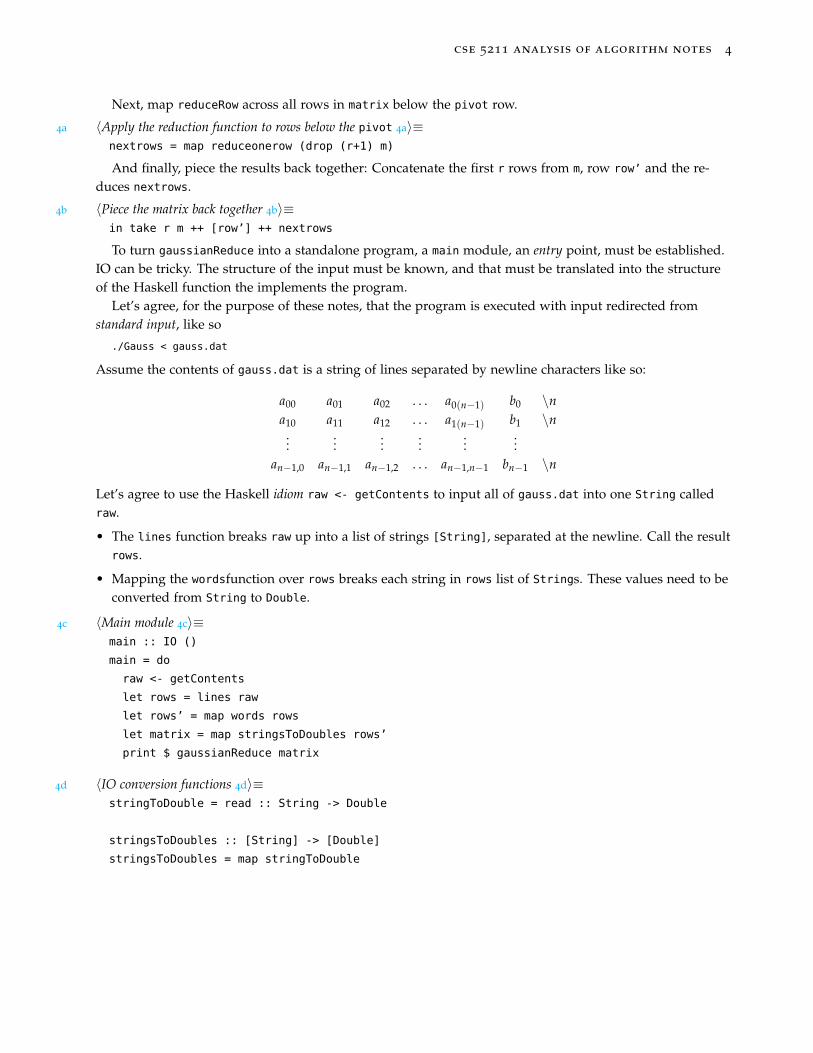
Next, map reduceRow across all rows in matrix below the pivot row.
4a 〈Apply the reduction function to rows below the pivot 4a〉≡nextrows = map reduceonerow (drop (r+1) m)
And finally, piece the results back together: Concatenate the first r rows from m, row row’ and the re-duces nextrows.
4b 〈Piece the matrix back together 4b〉≡in take r m ++ [row’] ++ nextrows
To turn gaussianReduce into a standalone program, a main module, an entry point, must be established.IO can be tricky. The structure of the input must be known, and that must be translated into the structureof the Haskell function the implements the program.
Let’s agree, for the purpose of these notes, that the program is executed with input redirected fromstandard input, like so
./Gauss < gauss.dat
Assume the contents of gauss.dat is a string of lines separated by newline characters like so:
a00 a01 a02 . . . a0(n−1) b0 \na10 a11 a12 . . . a1(n−1) b1 \n...
......
......
...an−1,0 an−1,1 an−1,2 . . . an−1,n−1 bn−1 \n
Let’s agree to use the Haskell idiom raw <- getContents to input all of gauss.dat into one String calledraw.
• The lines function breaks raw up into a list of strings [String], separated at the newline. Call the resultrows.
• Mapping the wordsfunction over rows breaks each string in rows list of Strings. These values need to beconverted from String to Double.
4c 〈Main module 4c〉≡main :: IO ()
main = do
raw <- getContents
let rows = lines raw
let rows’ = map words rows
let matrix = map stringsToDoubles rows’
print $ gaussianReduce matrix
4d 〈IO conversion functions 4d〉≡stringToDouble = read :: String -> Double
stringsToDoubles :: [String] -> [Double]
stringsToDoubles = map stringToDouble
cse 5211 analysis of algorithm notes 5
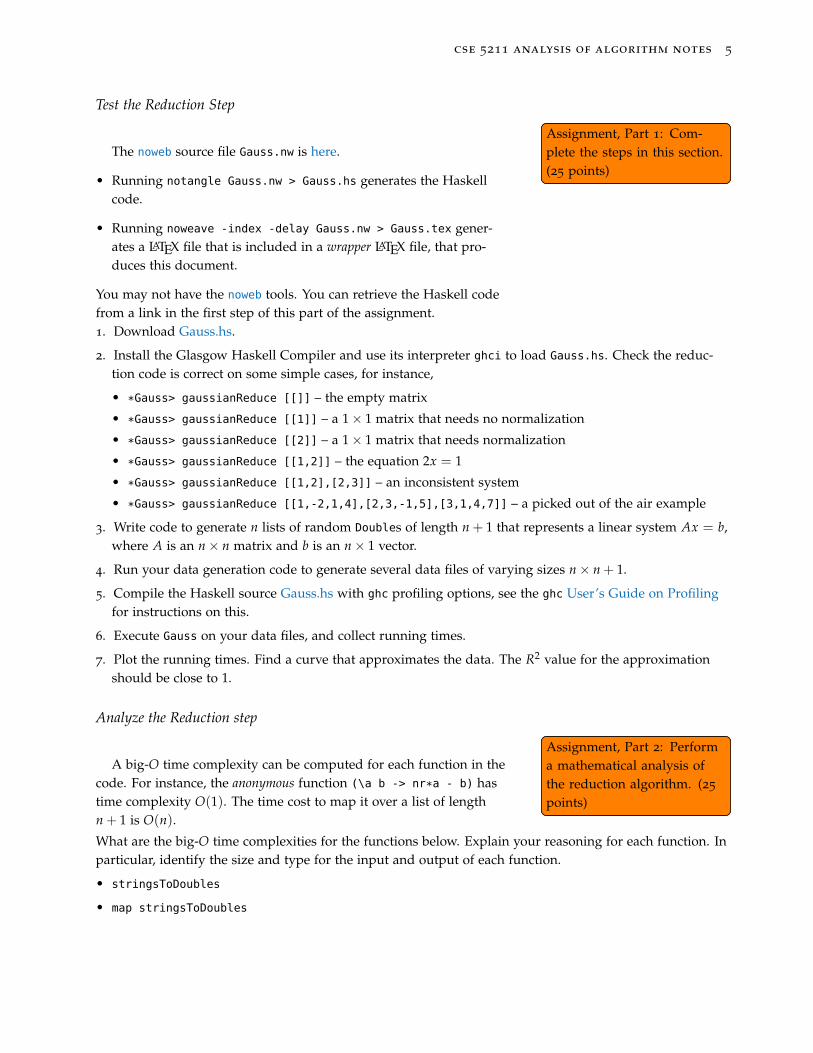
Test the Reduction Step
Assignment, Part 1: Com-plete the steps in this section.(25 points)
Assignment, Part 1: Com-plete the steps in this section.(25 points)
The noweb source file Gauss.nw is here.
• Running notangle Gauss.nw > Gauss.hs generates the Haskellcode.
• Running noweave -index -delay Gauss.nw > Gauss.tex gener-ates a LATEX file that is included in a wrapper LATEX file, that pro-duces this document.
You may not have the noweb tools. You can retrieve the Haskell codefrom a link in the first step of this part of the assignment.1. Download Gauss.hs.
2. Install the Glasgow Haskell Compiler and use its interpreter ghci to load Gauss.hs. Check the reduc-tion code is correct on some simple cases, for instance,
• *Gauss> gaussianReduce [[]] – the empty matrix
• *Gauss> gaussianReduce [[1]] – a 1× 1 matrix that needs no normalization
• *Gauss> gaussianReduce [[2]] – a 1× 1 matrix that needs normalization
• *Gauss> gaussianReduce [[1,2]] – the equation 2x = 1
• *Gauss> gaussianReduce [[1,2],[2,3]] – an inconsistent system
• *Gauss> gaussianReduce [[1,-2,1,4],[2,3,-1,5],[3,1,4,7]] – a picked out of the air example
3. Write code to generate n lists of random Doubles of length n + 1 that represents a linear system Ax = b,where A is an n× n matrix and b is an n× 1 vector.
4. Run your data generation code to generate several data files of varying sizes n× n + 1.
5. Compile the Haskell source Gauss.hs with ghc profiling options, see the ghc User’s Guide on Profilingfor instructions on this.
6. Execute Gauss on your data files, and collect running times.
7. Plot the running times. Find a curve that approximates the data. The R2 value for the approximationshould be close to 1.
Analyze the Reduction step
Assignment, Part 2: Performa mathematical analysis ofthe reduction algorithm. (25
points)
Assignment, Part 2: Performa mathematical analysis ofthe reduction algorithm. (25
points)
A big-O time complexity can be computed for each function in thecode. For instance, the anonymous function (\a b -> nr*a - b) hastime complexity O(1). The time cost to map it over a list of lengthn + 1 is O(n).
What are the big-O time complexities for the functions below. Explain your reasoning for each function. Inparticular, identify the size and type for the input and output of each function.
• stringsToDoubles
• map stringsToDoubles
cse 5211 analysis of algorithm notes 6
• reduceonerow
• reduceRow
• take r m ++ [row’] ++ nextrows
• gaussianReduce
Does the empirical run time data from experiments in you performed when testing gaussianReduce agreewith the analytic analysis?
The Gaussian Solver
Assignment, Part 3: Com-plete the Gaussian elimi-nation algorithm by imple-menting the solver step. (25
points)
Assignment, Part 3: Com-plete the Gaussian elimi-nation algorithm by imple-menting the solver step. (25
points)
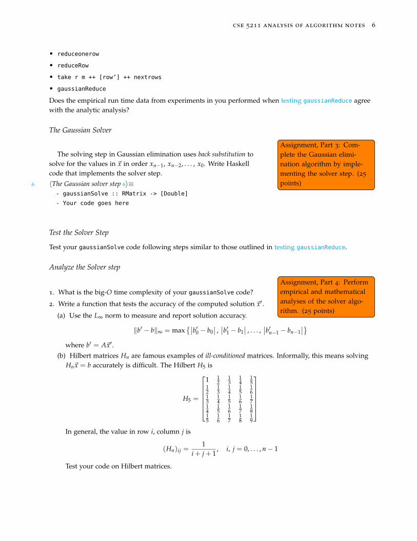
The solving step in Gaussian elimination uses back substitution tosolve for the values in ~x in order xn−1, xn−2, . . . , x0. Write Haskellcode that implements the solver step.
6 〈The Gaussian solver step 6〉≡- gaussianSolve :: RMatrix -> [Double]
- Your code goes here
Test the Solver Step
Test your gaussianSolve code following steps similar to those outlined in testing gaussianReduce.
Analyze the Solver step
Assignment, Part 4: Performempirical and mathematicalanalyses of the solver algo-rithm. (25 points)
Assignment, Part 4: Performempirical and mathematicalanalyses of the solver algo-rithm. (25 points)
1. What is the big-O time complexity of your gaussianSolve code?
2. Write a function that tests the accuracy of the computed solution ~x′.
(a) Use the L∞ norm to measure and report solution accuracy.
‖b′ − b‖∞ = max∣∣b′0 − b0
∣∣ ,∣∣b′1 − b1
∣∣ , . . . ,∣∣b′n−1 − bn−1
∣∣where b′ = A~x′.
(b) Hilbert matrices Hn are famous examples of ill-conditioned matrices. Informally, this means solvingHn~x = b accurately is difficult. The Hilbert H5 is
H5 =
1 1
213
14
15
12
13
14
15
16
13
14
15
16
17
14
15
16
17
18
15
16
17
18
19
In general, the value in row i, column j is
(Hn)ij =1
i + j + 1, i, j = 0, . . . , n− 1
Test your code on Hilbert matrices.

cse 5211 analysis of algorithm notes 7
References
Jones, S. P., editor (2002). Haskell 98 Language and Libraries: The Revised Report. http://haskell.org/.
Lipovaca, M. (2011). Learn You a Haskell for Great Good!: A Beginner’s Guide. No Starch Press, San Francisco,CA, USA, 1st edition.
The GHC Team (2014). The Glorious Glasgow Haskell Compilation System User’s Guide.

cse 5211 analysis of algorithm notes 8
Team Assignment
One quarter of a student’s course grade is based on team performance.
• Canvas will randomly generate three person teams. If enrollment is 3k + 1 there will be 2 two-personteams. If enrollment is 3k + 2 there will be 1 two-person team.
• Each team must schedule regular meetings of its members, bi-weekly at least.
– The team will choose a topic to research from the list below. Notify the instructor of the team’s choiceby email (mailto:[email protected]) on Monday of week 3 (Jan, 22). Requests will be granted first-come,first-serve. If a collision occurs the latter team must choose another available topic.
– On Mondays of weeks 5 (Feb, 5), 8 (Feb, 26), 10 (Mar, 12), and 12 (Mar, 26) the team must email a sta-tus report to (mailto:[email protected]). The report must outline who has researched, read, written, . . . ,what. Software development, mathematical analysis, and presentation outlines should be reported.
– On Wednesdays and Fridays of weeks: 5, 8, and 12, teams schedule review meeting with the instruc-tor during office hours: 9:30 – 10:50 or by appointment.
Potential Team Projects
Some of these topics are algorithms, others are data structures that support algorithms, and some are prob-lems where the algorithm is unspecified.
• Aho – Corasick algorithm
• B-trees
• Binomial heaps
• Boyer – Moore algorithm
• Cocke – Younger – Kasami (CYK) algorithm
• Euclidean GCD algorithm
• Fibonacci heaps
• Ford – Fulkerson maximum flow
• Gale – Shapley stable matching
• Huffman codes
• k-nearest neighbors
• Knuth – Morris – Pratt algorithm
• Longest common subsequence
• Miller – Rabin primality test
• Multiprocessor scheduling
• Needleman – Wunsch alignment
• QR matrix decomposition
• Rabin – Karp string search
• Red–Black trees
• Secure hash functions
• Set covers
• Simplex algorithm
• Singular value decomposition
• Strassen’s matrix multiplication algorithm
• Suffix trees
• Transitive closures
• Traveling salesman
• Union-Find for disjoint sets
• Vertex covers
• Skip lists
Team and Presentation Advice
Guidelines from Teamwork in the Classroom:

cse 5211 analysis of algorithm notes 9
• Have clear goals
• Be results-driven
• Be a competent member
• Be committed to the goal
• Collaborate
• Have high standards
• Follow principled leadership
• Seek support, advice, and encouragement
A summary of Tufte’s tips for a successful presentation:
• Show up early
• Lay out the problem
• Present complicated material in order par-ticular, general, particular, . . .
• Avoid an obvious reliance on notes
• Give everyone in your audience a piece ofpaper
• Match the information density to the allotedtime
• Avoid overhead projectors, keep the lightson
• Never apologize
• Use (relevant, never irritating) humor
• Use gender-neutral speech
• Practice intensely beforehand
• Take questions without condescending
• Express (real) enthusiasm
• Finish early
Presentation schedule
The team must provide classmates with a one page, double sided handout highlighting the main results oftheir research. Every team member must participate in discussing the team’s work.
• Monday of week 15 (Apr, 16): Team 1 & 2
• Wednesday of week 15 (Apr, 18): Team 3 & 4
• Friday of week 15 (Apr, 18): Team 5 & 6
• Monday of week 16 (Apr, 23): Team 7 & 8
Final submission
On or before Wednesday of week 16 (Apr, 25) the team must submit on Canvas:
• The handout prepared for classmates
• Slides prepared for the presentation
• Code written, scripts (instructions) for compiling and executing your program, and test data
• A final report summarizing the work: The problem, the algorithm, the analysis, the experiments, thesummary, and the references
On or before Wednesday of week 15 (Apr, 25) each student complete:
• A performance evaluation of their teammates
• An evaluation of presentations by other teams
cse 5211 analysis of algorithm notes 10
Questions and Problems
Here’s collection of exercises are serve to outline topics and what students are expected to know by the endof the course.
Theory
1. What is a (deterministic) Turing machine?
2. What is a non-deterministic Turing machine?
3. Are there decision problems whose answers (“yes” or “no”) are unknown? Be able to explain your answer.
4. Are there decision problems that have no algorithm? Be able to explain your answer.
5. Are there decision problems where it is unknown whether or not an algorithm exists? Be able to explainyour answer.
6. What is the key difference between decision problems and function problems?
7. Other than time and space, what other resources are consumed when an algorithm executes?
Asymptotic Notation
1. A running time (complexity) function f : X 7→ Y that defines a class O( f (x)) should have certainproperties: What would you choose for:
(a) X, the domain of f ?
(b) Y, the range of f ?
(c) The monotonicity of f ?
(d) The computability of f ?
(e) The time complexity of computing f (x)?
(f) The space complexity of computing f (x)?
2. Define the class of running time functions O(n2).
3. Find witnesses that show the following:
(a) 5n + 6 = O(n2)
(b) 3n2 + n + 6 = O(n2)
4. Find witnesses that show the following:
(a) 3n2 + n + 6 = Θ(n2)
(b) logb1x = Θ(logb2
x) for bases b1, b2 > 1.
5. True or False: All exponentials grow at the same rate: Is 2n = Θ(bn) for every base b > 1?
6. Assume f (n) ∈ O(g(n)). Prove or disprove:
(a) f (n)2 = O(g(n)2)
(b) lg f (n) = O(lg g(n))
(c) 2 f (n) = O(2g(n))
(d) f (n) lg f (n) = O(g(n) lg g(n))
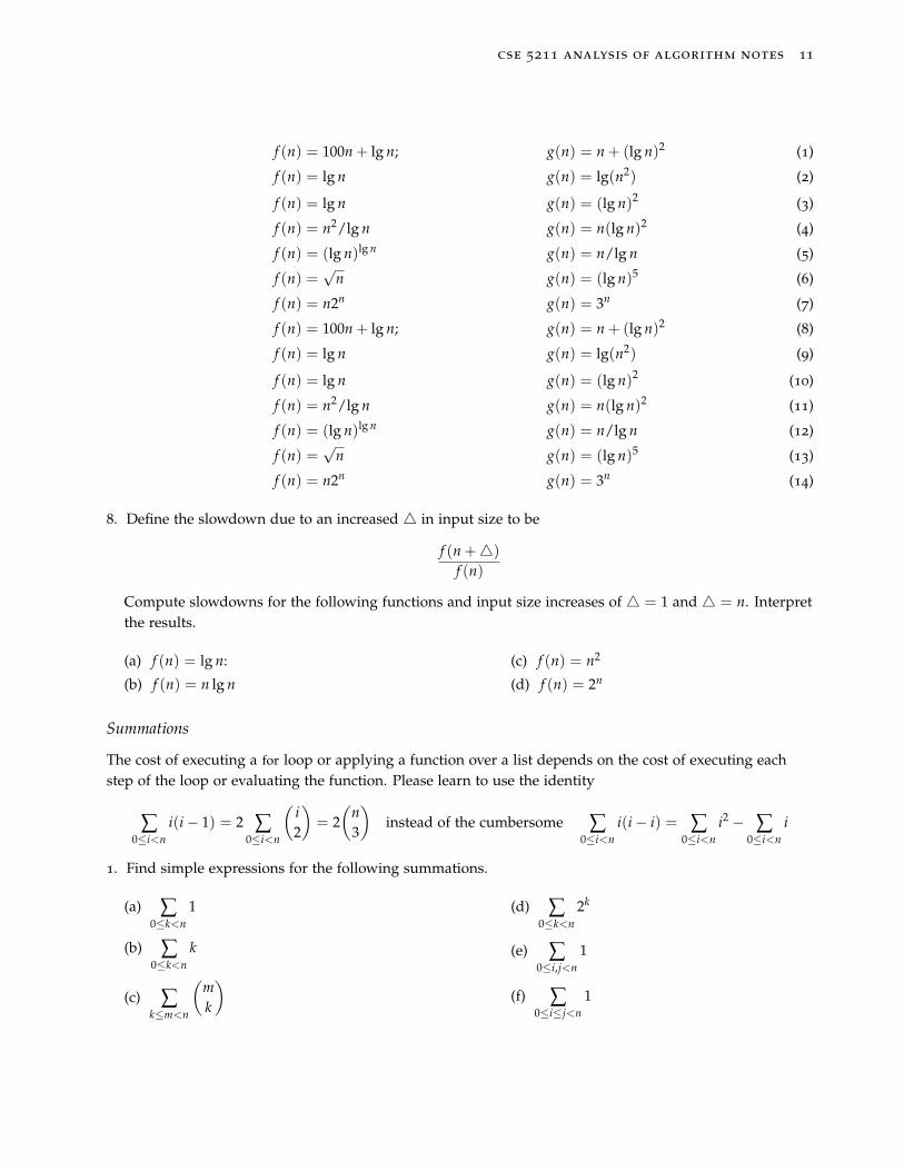
7. For each of the following pairs of functions f and g, indicate whether f (n) = O(g(n)), f (n) = Ω(g(n)),or both (i.e., f (n) = Θ(g(n)).)
cse 5211 analysis of algorithm notes 11
f (n) = 100n + lg n; g(n) = n + (lg n)2 (1)
f (n) = lg n g(n) = lg(n2) (2)
f (n) = lg n g(n) = (lg n)2 (3)
f (n) = n2/lg n g(n) = n(lg n)2 (4)
f (n) = (lg n)lg n g(n) = n/lg n (5)
f (n) =√
n g(n) = (lg n)5 (6)
f (n) = n2n g(n) = 3n (7)
f (n) = 100n + lg n; g(n) = n + (lg n)2 (8)
f (n) = lg n g(n) = lg(n2) (9)
f (n) = lg n g(n) = (lg n)2 (10)
f (n) = n2/lg n g(n) = n(lg n)2 (11)
f (n) = (lg n)lg n g(n) = n/lg n (12)
f (n) =√
n g(n) = (lg n)5 (13)
f (n) = n2n g(n) = 3n (14)
8. Define the slowdown due to an increased 4 in input size to be
f (n +4)
f (n)
Compute slowdowns for the following functions and input size increases of 4 = 1 and 4 = n. Interpretthe results.
(a) f (n) = lg n:
(b) f (n) = n lg n
(c) f (n) = n2
(d) f (n) = 2n
Summations
The cost of executing a for loop or applying a function over a list depends on the cost of executing eachstep of the loop or evaluating the function. Please learn to use the identity
∑0≤i<n
i(i− 1) = 2 ∑0≤i<n
(i2
)= 2
(n3
)instead of the cumbersome ∑
0≤i<ni(i− i) = ∑
0≤i<ni2 − ∑
0≤i<ni
1. Find simple expressions for the following summations.
(a) ∑0≤k<n
1
(b) ∑0≤k<n
k
(c) ∑k≤m<n
(mk
)
(d) ∑0≤k<n
2k
(e) ∑0≤i,j<n
1
(f) ∑0≤i≤j<n
1
cse 5211 analysis of algorithm notes 12
(g) ∑0≤i,j,k<n
1
(h) ∑0≤i≤j≤k<n
1
(i) ∑0≤i≤n
i(n− i)
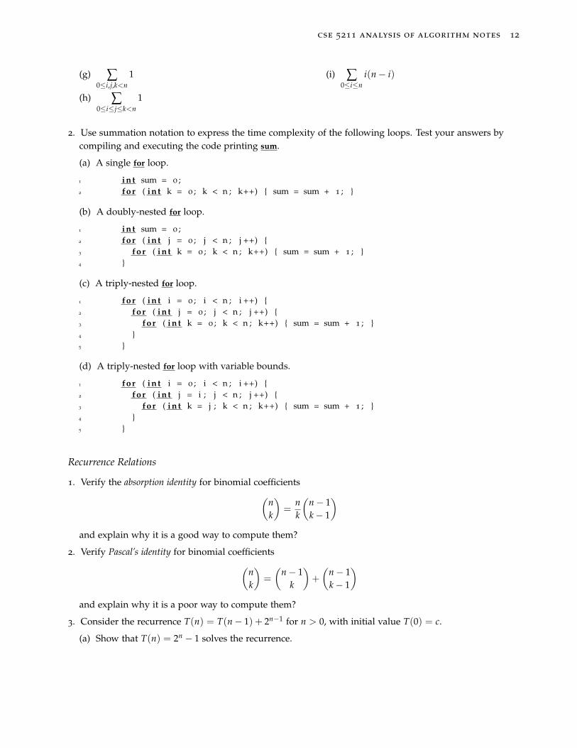
2. Use summation notation to express the time complexity of the following loops. Test your answers bycompiling and executing the code printing sum.
(a) A single for loop.
1 i n t sum = 0 ;2 for ( i n t k = 0 ; k < n ; k++) sum = sum + 1 ;
(b) A doubly-nested for loop.
1 i n t sum = 0 ;2 for ( i n t j = 0 ; j < n ; j ++) 3 for ( i n t k = 0 ; k < n ; k++) sum = sum + 1 ; 4
(c) A triply-nested for loop.
1 for ( i n t i = 0 ; i < n ; i ++) 2 for ( i n t j = 0 ; j < n ; j ++) 3 for ( i n t k = 0 ; k < n ; k++) sum = sum + 1 ; 4 5
(d) A triply-nested for loop with variable bounds.
1 for ( i n t i = 0 ; i < n ; i ++) 2 for ( i n t j = i ; j < n ; j ++) 3 for ( i n t k = j ; k < n ; k++) sum = sum + 1 ; 4 5
Recurrence Relations
1. Verify the absorption identity for binomial coefficients(nk
)=
nk
(n− 1k− 1
)and explain why it is a good way to compute them?
2. Verify Pascal’s identity for binomial coefficients(nk
)=
(n− 1
k
)+
(n− 1k− 1
)and explain why it is a poor way to compute them?
3. Consider the recurrence T(n) = T(n− 1) + 2n−1 for n > 0, with initial value T(0) = c.
(a) Show that T(n) = 2n − 1 solves the recurrence.
cse 5211 analysis of algorithm notes 13
(b) Show how to solve the recurrence T(n) = T(n− 1) + 2n−1, with initial value T(0) = c. by summingthe telescoping sum T(k)− T(k− 1) for k = 0 to k = n.
4. Consider the recurrence T(n) = 3T(n− 1) + 4T(n− 2).
(a) Solve the characteristic polynomial x2 = 3x− 4
(b) Show that T(n) = 4n + (−1)n solves the recurrence
5. Analyze the complexity of the algorithm
1 schedule : : [ ( Int , Int ) ] −> [ ( Int , Int ) ]2 schedule [ ] = [ ]3 schedule [ ( s , f ) ] = [ ( s , f ) ]4 schedule [ ( s0 , f0 ) , ( s1 , f1 ) : r e s t ] =5 | s1 >= f0 = [ ( s0 , f0 ) , ( s1 , f1 ) ] ++ schedule [ ( s1 , f1 ) : r e s t ]6 | otherwise schedule [ ( s0 , f0 ) : r e s t ]
Generating Functions
1. Two fundamental generating functions are:
11− z
= ∑k≥0
zk = ∑k≥0
(k + 0
0
)zk and
1(1− z)2 = ∑
k≥0kzk−1 = ∑
k≥0
(k + 1
1
)zk
Use induction to show1
(1− z)n+1 = ∑k≥0
(k + n
n
)zk
2. Use generating functions to show Mn = 2n − 1 solves the Mersenne recurrence Mn = 2Mn−1 + 1,M0 = 0.
3. Show how to solve the recurrence T(n) = T(n− 1) + 2n−1 by generating functions.
4. Use generating functions to find the solution to the recurrence T(n) = 3T(n− 1) + 4T(n− 2).
5. What function generates the sequence 〈1, 0, 1, 0, . . .〉?
Divide-and-Conquer Algorithms
Greedy Algorithms
1. The minimal spanning tree problem is: Given a graph G = (V, E) with n vertices and edge weightsw(i, j) > 0 for (i, j) ∈ E. Find a spanning tree T that minimized the weight of the tree
w(T) = ∑(i, j)∈E
w(i, j)
(a) What are the characteristics of a spanning tree T?
(b) One greedy heuristic is to process the edges in order of increasing cost: Start with an empty treeT = ∅. If edge e = (i, j) does not contain a cycle when added to T, let T = T ∪ e until T containsn− 1 edges.
2. Consider the traveling salesman problem.
cse 5211 analysis of algorithm notes 14
(a) Describe a greedy heuristic that could be used to find an Hamiltonian cycle that approximates anoptimal salesman’s cycle.
(b) Construct example weighted graphs where the greedy heuristic does and does not find an optimalHamiltonian cycle.
Dynamic Programming
1. The dynamic programming paradigm requires computing values in an n× m matrix with values An,m.To order of computation depends on the recurrence that describes An,m in terms of previously computedvalues. This dependence is typically by column
Ai, j i = 0, . . . , (n− 1), j = 0, . . . , (m− 1)
by rowAi, j j = 0, . . . , (m− 1), i = 0, . . . , (n− 1)
or, by diagonalAi, j i + j = 0, . . . , n + m− 2)
(a) What is the time complexity of a dynamic programming algorithm where each value in A can becomputed in O(1) time?
(b) Sometimes only values in the upper (or lower) triangle of A need to be computed. How does thisalter the answer to the previous question?
(c) What nested for loops fill A by columns order?
(d) What nested for loops fill A by rows order?
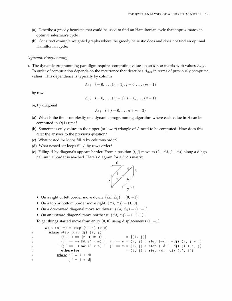
(e) Filling A by diagonals appears harder. From a position (i, j) move to (i +4i, j +4j) along a diago-nal until a border is reached. Here’s diagram for a 3× 3 matrix.
0
12
3
4
5
6
7
• On a right or left border move down: (4i, 4j) = (0, −1).
• On a top or bottom border move right: (4i, 4j) = (1, 0).
• On a downward diagonal move southwest: (4i, 4j) = (1, −1).
• On an upward diagonal move northeast: (4i, 4j) = (−1, 1).
To get things started move from entry (0, 0) using displacements (1, −1)
1 walk ( n , m) = step (1 ,−1) ( 0 , 0 )2 where s tep ( di , d j ) ( i , j )3 | ( i , j ) == ( n−1 , m−1) = [ ( i , j ) ]4 | ( i ’ == −1 && j ’ < m) || i ’ == n = ( i , j ) : s tep (−di , −dj ) ( i , j + 1 )5 | ( j ’ == −1 && i ’ < n ) || j ’ == m = ( i , j ) : s tep (−di , −dj ) ( i + 1 , j )6 | otherwise = ( i , j ) : s tep ( di , d j ) ( i ’ , j ’ )7 where i ’ = i + di8 j ’ = j + d j
cse 5211 analysis of algorithm notes 15
Load the code in the ghci interpreter and verify it correctly walks a matrix in diagonal order.
(f) In some problems, the number of columns, m, in A is a bound on a constraint that any solution mustsatisfy. In these cases, the input size is taken to be blg mc+ 1, the minimal number of bits needed tostore m. How does this alter the interpretation of the answer to problem 1a? question?
2. The 0–1 knapsack problem is: Given weights wi and profits pi, 0 ≤ i < n, and a capacity M, find optimalpacking of the knapsack. Let P[j, m] be the profit of an optimal solution using provisions 0, . . . , j andknapsack capacity m.
(a) Write a dynamic programming algorithm for computing P[n − 1, M], the maximum value of theoptimal solution. The recursion to use has initial conditions
P[0, m] =
0 if w0 > m
p0 if w0 ≤ m
and recurrence
P[j, m] =
P[j− 1, m] if wj > m
max
P[j− 1, m], pj + P[j− 1, m− wj]
if wj ≤ m(1 ≤ j < n and 0 ≤ m ≤ M)
(b) What rows and columns does the the computation of P[j, m] depend upon?
(c) What is the time complexity of your algorithm?
(d) Is the time complexity polynomial or exponential in the number of provisions and the capacity (nand M)?
(e) What would the time complexity be if, instead of storing values P[i, j] in a look-up (memoized)matrix, these values were computed by recursive functions calls?
3. The matrix chain product problem is: Given matrices M0, M1, . . . , Mn−1. Find an optimal way to paren-thesize the product M0 ·M1 · · ·Mn−1 to minimize the number of scalar multiplications.
(a) Show that the Catalan number
Cn−1 =1n
(2n− 2n− 1
)counts the number of different ways to parenthesize n matrices.
(b) Write a dynamic programming algorithm for computing C[0, n], the minimal value of the optimalsolution. The recursion to use has initial conditions
C[j, j] = 0 for 0 ≤ j ≤ n− 1
and recurrence
C[j, k] = min
C[j, i] + C[i + 1, k] + rj · ci · ck : j ≤ i ≤ k− 1
(1 ≤ j < n, 0 ≤ k ≤ M)
(c) What rows and columns does the the computation of C[j, k] depend upon? A matrix layout diagramwould be a good way to explain an answer.
(d) Show that the sum
∑j≤i<k
1 (models the time cost of computing C[j, k])
(e) What is the time complexity of your algorithm?

cse 5211 analysis of algorithm notes 16
(f) What would the time complexity be if, instead of storing values C[j, k] in a look-up (memoized)matrix, these values were computed by recursive functions calls?
4. The traveling salesman problem is: Given an undirected graph G = (V, E) on n vertices and weightsw(i, j) > 0 for each edge (i, j) ∈ E. Find a minimal cost Hamiltonian cycle H, a closed loop, starts atvertex 0 and visits every other node exactly once returning to 0.
For notation,
• Let S be a subset of 1, . . . , n− 1• Let P[S, k] be the cost of an optimal path from vertex 0 to vertex k, where all intermediate vertices lie
in S.
(a) Explain why min P[V − 0 , k] : 1 ≤ k < n is the cost of an optimal salesman’s cycle.
(b) Explain why the recursion with initial conditions
P[k , k] = w(0, k), 1 ≤ k < n
and recurrence
P[S, k] = min P[S− k , m] + w(m, k) : m ∈ S− k (if |S| > 1)
describes the construction of optimal solutions.
(c) Write a dynamic programming algorithm for the traveling salesman problem. Your algorithm willcalculate the values P[S, k] in order of increasing cardinality: |S| = 1, |S| = 2, . . . , |S| = n− 1
(d) What is the time complexity of your algorithm?
Numerics
1. Let ω = e−2πi1/4 be the principle 4-th root of unity.
(a) Show that ω2 = e−πi = −1.
(b) Let m = 2k + r and show ωm = ω2k+r = (−1)kωr
Backtracking
Complexity and Computability
Answer True or False for the following sentences, or explain that the answer is unknown.
1. All NP-hard problems are NP-complete.
2. The set of NP-complete problems is a subset of NP.
3. NP-complete problems cannot have polynomial algorithms.
4. In order to prove a problem X to be NP-complete one needs to develop a polynomial transformationfrom a known NP-complete problem to X.
5. 2-SAT is an NP-hard problem.
6. There is a non-deterministic polynomial time algorithm that decides the halting problem.
7. This sentence is False.
cse 5211 analysis of algorithm notes 17
Logic and algorithm share the notions of “expression” and “type”, whose form ismade precise by the syntax.
Wikipedia: Hindley–Milner type system
Algorithms
The word algorithm has several interpretations. A formal definition might be: An algorithm isa Turing machine M that always halts when executed with w written on M’s input tape. The output u, iswhat is written on the tape when M halts. Every Turing machine that always halts on its input specifiessome algorithm. (Knuth, 1997) says, an algorithm has these properties:
• Finiteness: An algorithm must always terminate after a finite number of steps
• Definiteness: Each step of an algorithm must be precisely defined; the actions to be carried out must berigorously and unambiguously specified for each case
• Input: Some quantities of known types are given before the algorithm begins
• Output: Some quantities of known types that have a specified relation to the inputs are computed
• Effectiveness: All of the operations to be performed must be sufficiently basic that they can in principlebe done exactly and in a finite time using paper and pencil
A prime consideration in the analysis of algorithms is the number of steps taken in computing the outputfrom the input. We’d like to bound the number of steps above and below by functions of input size. We’dalso like to know how the algorithm behaves on average given a distribution of input values.
Decision and Function Problems
Algorithms are used to solve problems. Decision problems and function problems are two problemclasses.
Decision problems are basic: A question that has a “yes” (True) or “no” (False) answer is a decision prob-lem. Consider the decision problem: Is a list of n numbers a0, a1, . . . , an−1 sorted?
Function problems require output that is more complex than “yes” or “no”. Function problems can some-times be reduced to solving a sequence of decision problems. Consider the function problem: Sort a listof n numbers a0, a1, . . . , an−1. The output is the sorted list aπ(k) ≤ aπ(k+1) for k = 0, . . . , (n − 1) whereπ : Zn 7→ Zn is a permutation, a one-to-one and onto function.
There are known problems for which there is no algorithm (assuming the Church–Turing hypothesis isTrue). The halting problem: Does Turing machine M halt on input w? is undecidable.
There are known problems for which it is not known if an algorithm exists or not: Is there an infinitenumber of twin-primes?
For the problems covered here, almost always there will be more than one algorithm. Since this is thecase, a method of comparing algorithms is sought.
• The number of steps (instructions) taken is one measure for comparison. The number of steps is calledthe time complex of the algorithm. This begs the question: How can a step be quantified?
cse 5211 analysis of algorithm notes 18
• The amount of memory used is another measure for comparison. The memory usage is called the spacecomplex of the algorithm. It is traditional to not include the input or output space in this measure. Onlythe extra space needed to implement the algorithm is counted. This may be a mistaken assumption inthe era of big data. Memory usage can be measured by the number of addresses: A uniform model. Or, itcan be measured logarithmically by the amount of memory at an address. (Think of a postman and maildelivery)
• In addition to time and space, what other resources might it be useful to measure?
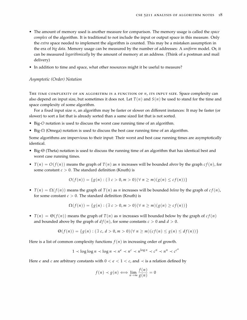
Asymptotic (Order) Notation
The time complexity of an algorithm is a function of n, its input size. Space complexity canalso depend on input size, but sometimes it does not. Let T(n) and S(n) be used to stand for the time andspace complexity of some algorithm.
For a fixed input size n, an algorithm may be faster or slower on different instances: It may be faster (orslower) to sort a list that is already sorted than a same sized list that is not sorted.
• Big-O notation is used to discuss the worst case running time of an algorithm.
• Big-Ω (Omega) notation is used to discuss the best case running time of an algorithm.
Some algorithms are impervious to their input: Their worst and best case running times are asymptoticallyidentical.
• Big-Θ (Theta) notation is used to discuss the running time of an algorithm that has identical best andworst case running times.
• T(n) = O( f (n)) means the graph of T(n) as n increases will be bounded above by the graph c f (n), forsome constant c > 0. The standard definition (Knuth) is
O( f (n)) = g(n) : (∃ c > 0, m > 0)(∀ n ≥ m)(g(n) ≤ c f (n))
• T(n) = Ω( f (n)) means the graph of T(n) as n increases will be bounded below by the graph of c f (n),for some constant c > 0. The standard definition (Knuth) is
Ω( f (n)) = g(n) : (∃ c > 0, m > 0)(∀ n ≥ m)(g(n) ≥ c f (n))
• T(n) = Θ( f (n)) means the graph of T(n) as n increases will bounded below by the graph of c f (n)and bounded above by the graph of d f (n), for some constants c > 0 and d > 0.
Θ( f (n)) = g(n) : (∃ c, d > 0, m > 0)(∀ n ≥ m)(c f (n) ≤ g(n) ≤ d f (n))
Here is a list of common complexity functions f (n) in increasing order of growth.
1 ≺ log log n ≺ log n ≺ nε ≺ nc ≺ nlog n ≺ cn ≺ nn ≺ ccn
Here ε and c are arbitrary constants with 0 < ε < 1 < c, and ≺ is a relation defined by
f (n) ≺ g(n) ⇐⇒ limn→∞
f (n)g(n)
= 0

cse 5211 analysis of algorithm notes 19
Courses on data structure teach methods to show a function g(n) is O( f (n)). Some methods are sim-ple. For instance,
n2 ≤ 3n2 + 5n + 2 ≤ (3 + 5 + 2)n2 = 10n2 shows 3n2 + 5n + 2 = Θ(n2)
Calculus concepts, limits and l’Hopital’s rule, can be useful for more difficult problems: When used toanalyze algorithms, the functions f (n) and g(n) grow without bound and l’Hopital’s rule states that when
limn→∞
f ′(n)g ′(n)
= L then limn→∞
f (n)g(n)
= L
References
Knuth, D. E. (1997). The Art of Computer Programming, Volume 1 (3rd Ed.): Fundamental Algorithms. AddisonWesley Longman Publishing Co., Inc., Redwood City, CA, USA. [page 17]

cse 5211 analysis of algorithm notes 20
Algorithm Design
Maximum Subsequence Sum Problem
This section is about algorithmic design. To gain a deeper understanding, read Jon Bentley’s Program-ming Pearl “Algorithm Design Techniques,” (Bentley, 1984) and §4.1 The maximum sub-array problem, inthe text (Corman et al., 2009).
Motivation for the problem comes from instances.
• Consider the Dow Jones Industrial Average: It goes up and down daily. What contiguous run of dayshas the highest gain? Consider your weight: It goes up and down daily. What contiguous run of dayshas the largest weight gain or loss?
• Consider the bitcoin market. It to has runs up and down.
A particular instance is the sequence of integers
X = [−1, −2, 3, 5, 6, −2, −1, 4, −4, 2, −1] of length n = 11.
By inspection you may notice the largest gain is 15 over the (contiguous) subsequence
[3, 5, 6, −2, −1, 4]
The empty sequence [] is a contiguous subsequence of X and the sum of elements in [] is 0. For n = 11there are 11 sums with 1 term, 10 sums with 2 terms, 9 sums with 3 terms, . . . , and 1 sum with 11 terms.Computing these sums can take up to
11 · 1 + 10 · 2 + 9 · 3 + · · ·+ 1 · 11 = 286 additions
∑0≤k≤n+1
(n− k)k =
(n + 1
3
)=
(n + 2)(n + 1)(n)6
= O(n3)
The maximum subsequence sum problem is: Given a list of integers X[k], k = 0, . . . , (n− 1), n ≥ 0, find themaximal value of
∑s≤k≤e
X[k] for 0 ≤ s ≤ e ≤ (n− 1).
In case all values in X are negative, the maximum subsequence sum is 0, from the empty subsequence.Let’s design some algorithms that solves the maximum subsequence sum problem.
Brute Force
,The brute-force approach computes the sum of every possible subsequence and remembers the largest.
Download the code here.
20 〈Cubic 20〉≡int maxSubseqSum(int X[], int n)
int MaxSoFar = 0; // local state
〈For each start of a subsequence 21a〉
〈For each end of the subsequence 21b〉
cse 5211 analysis of algorithm notes 21
int Sum = 0; // More local state
〈For each subsequence 21c〉
〈Compute partial sum; Check MaxSoFar 21d〉
return MaxSoFar;
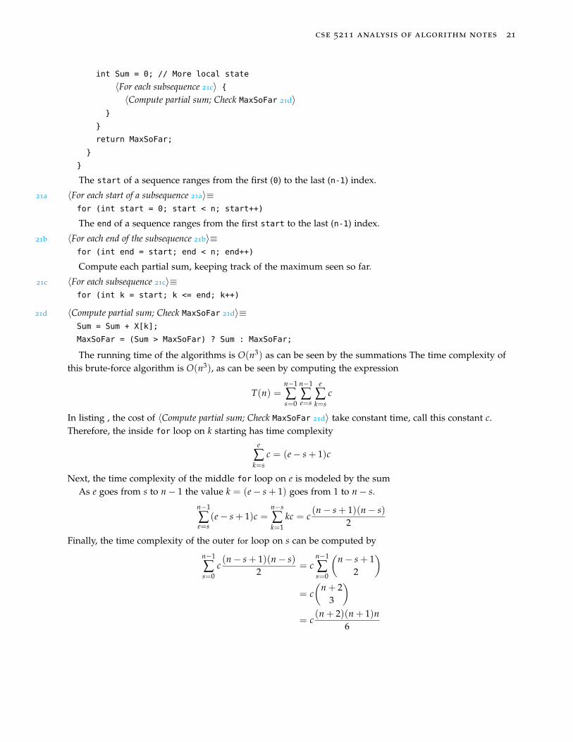
The start of a sequence ranges from the first (0) to the last (n-1) index.
21a 〈For each start of a subsequence 21a〉≡for (int start = 0; start < n; start++)
The end of a sequence ranges from the first start to the last (n-1) index.
21b 〈For each end of the subsequence 21b〉≡for (int end = start; end < n; end++)
Compute each partial sum, keeping track of the maximum seen so far.
21c 〈For each subsequence 21c〉≡for (int k = start; k <= end; k++)
21d 〈Compute partial sum; Check MaxSoFar 21d〉≡Sum = Sum + X[k];
MaxSoFar = (Sum > MaxSoFar) ? Sum : MaxSoFar;
The running time of the algorithms is O(n3) as can be seen by the summations The time complexity ofthis brute-force algorithm is O(n3), as can be seen by computing the expression
T(n) =n−1
∑s=0
n−1
∑e=s
e
∑k=s
c
In listing , the cost of 〈Compute partial sum; Check MaxSoFar 21d〉 take constant time, call this constant c.Therefore, the inside for loop on k starting has time complexity
e
∑k=s
c = (e− s + 1)c
Next, the time complexity of the middle for loop on e is modeled by the sumAs e goes from s to n− 1 the value k = (e− s + 1) goes from 1 to n− s.
n−1
∑e=s
(e− s + 1)c =n−s
∑k=1
kc = c(n− s + 1)(n− s)
2
Finally, the time complexity of the outer for loop on s can be computed by
n−1
∑s=0
c(n− s + 1)(n− s)
2= c
n−1
∑s=0
(n− s + 1
2
)= c(
n + 23
)= c
(n + 2)(n + 1)n6
cse 5211 analysis of algorithm notes 22
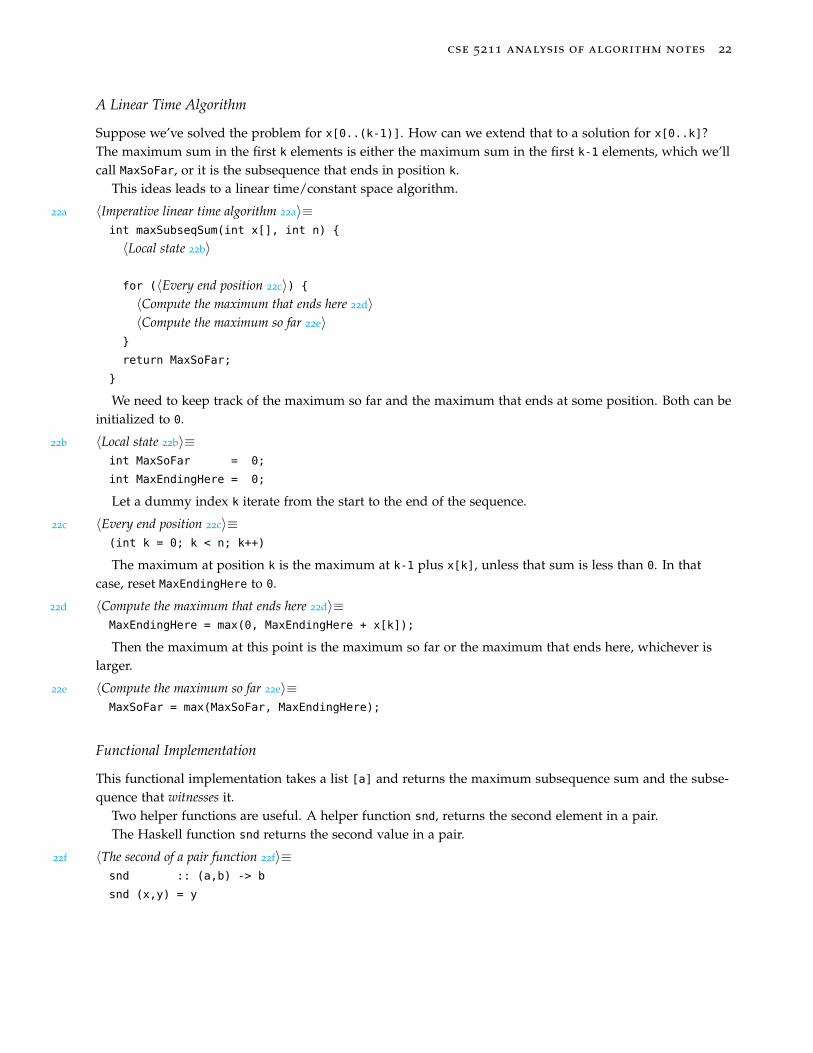
A Linear Time Algorithm
Suppose we’ve solved the problem for x[0..(k-1)]. How can we extend that to a solution for x[0..k]?The maximum sum in the first k elements is either the maximum sum in the first k-1 elements, which we’llcall MaxSoFar, or it is the subsequence that ends in position k.
This ideas leads to a linear time/constant space algorithm.
22a 〈Imperative linear time algorithm 22a〉≡int maxSubseqSum(int x[], int n)
〈Local state 22b〉
for (〈Every end position 22c〉)
〈Compute the maximum that ends here 22d〉〈Compute the maximum so far 22e〉
return MaxSoFar;
We need to keep track of the maximum so far and the maximum that ends at some position. Both can beinitialized to 0.
22b 〈Local state 22b〉≡int MaxSoFar = 0;
int MaxEndingHere = 0;
Let a dummy index k iterate from the start to the end of the sequence.
22c 〈Every end position 22c〉≡(int k = 0; k < n; k++)
The maximum at position k is the maximum at k-1 plus x[k], unless that sum is less than 0. In thatcase, reset MaxEndingHere to 0.
22d 〈Compute the maximum that ends here 22d〉≡MaxEndingHere = max(0, MaxEndingHere + x[k]);
Then the maximum at this point is the maximum so far or the maximum that ends here, whichever islarger.
22e 〈Compute the maximum so far 22e〉≡MaxSoFar = max(MaxSoFar, MaxEndingHere);
Functional Implementation
This functional implementation takes a list [a] and returns the maximum subsequence sum and the subse-quence that witnesses it.
Two helper functions are useful. A helper function snd, returns the second element in a pair.The Haskell function snd returns the second value in a pair.
22f 〈The second of a pair function 22f〉≡snd :: (a,b) -> b
snd (x,y) = y
cse 5211 analysis of algorithm notes 23
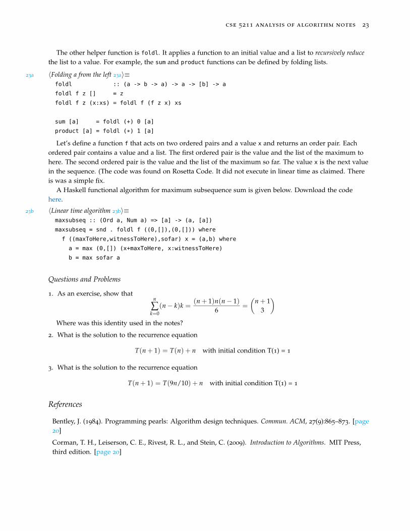
The other helper function is foldl. It applies a function to an initial value and a list to recursively reducethe list to a value. For example, the sum and product functions can be defined by folding lists.
23a 〈Folding a from the left 23a〉≡foldl :: (a -> b -> a) -> a -> [b] -> a
foldl f z [] = z
foldl f z (x:xs) = foldl f (f z x) xs
sum [a] = foldl (+) 0 [a]
product [a] = foldl (*) 1 [a]
Let’s define a function f that acts on two ordered pairs and a value x and returns an order pair. Eachordered pair contains a value and a list. The first ordered pair is the value and the list of the maximum tohere. The second ordered pair is the value and the list of the maximum so far. The value x is the next valuein the sequence. (The code was found on Rosetta Code. It did not execute in linear time as claimed. Thereis was a simple fix.
A Haskell functional algorithm for maximum subsequence sum is given below. Download the codehere.
23b 〈Linear time algorithm 23b〉≡maxsubseq :: (Ord a, Num a) => [a] -> (a, [a])
maxsubseq = snd . foldl f ((0,[]),(0,[])) where
f ((maxToHere,witnessToHere),sofar) x = (a,b) where
a = max (0,[]) (x+maxToHere, x:witnessToHere)
b = max sofar a
Questions and Problems
1. As an exercise, show thatn
∑k=0
(n− k)k =(n + 1)n(n− 1)
6=
(n + 1
3
)Where was this identity used in the notes?
2. What is the solution to the recurrence equation
T(n + 1) = T(n) + n with initial condition T(1) = 1
3. What is the solution to the recurrence equation
T(n + 1) = T(9n/10) + n with initial condition T(1) = 1
References
Bentley, J. (1984). Programming pearls: Algorithm design techniques. Commun. ACM, 27(9):865–873. [page20]
Corman, T. H., Leiserson, C. E., Rivest, R. L., and Stein, C. (2009). Introduction to Algorithms. MIT Press,third edition. [page 20]
cse 5211 analysis of algorithm notes 24
Mathematical Tools
To analyze algorithms requires skills. Some of these are mathematical.
Summations
Mastery of summations is a fundamental skill. (Graham et al., 1989) is a great source for summations.Summations are discrete analogs of integrals from continuous mathematics. There are many useful sum-mations. Here are a few. Mathematical induction can be used to prove they are correct.
• Tally sums:
∑0≤k<j
m = mj sums along a flat line increase linearly.
Code template:
1 f o r ( i n t k = 0 ; k < j ; k++) sum = sum + k ;
• Arithmetic sums:
∑0≤j<n
(mj + b) = m(
n2
)+ nb sums along a sloped line increase quadratically.
Code template:
1 f o r ( i n t j = n−1; j > 0 ; j−− ) 2 f o r ( i n t k = 1 ; k <= j ; k++) 3 i f (A[ k−1] > A[ k ] ) swap (A[ k−1] , A[ k ] ) ; 4 5
• Binomial coefficients column sums generalize the above results to higher dimensions. Let the column befixed at m, and sum binomial coefficients
∑0≤i≤n
(im
)=
(n + 1m + 1
); When m = 2, ∑
0≤i≤n
(i2
)=
(n + 1
3
)Code template:
1 f o r ( i n t i = 0 ; i < n ; i ++) 2 f o r ( i n t j = 0 ; j < i ; j ++) 3 f o r ( i n t k = 0 ; k < j ; k++) O(1) operat ion ; 4 5
• Geometric sums
∑0≤k<n
(1 + r)k =(1 + r)n − 1
rsum along an exponential
Good for earning money, bad for time complexity.

cse 5211 analysis of algorithm notes 25
Recursion
Recursion is a common problem solving strategy. Express a solution in terms of solutions toreduced problems. Recurrence equations are discrete analogs of differential equations from continuousmathematics.
There are many useful recurrences and simple functions that satisfy them. There is a master theorem thatsummarizes many cases. You can always look it up. I prefer to know the basic rules that lead to it.
• Pretend n is a power of 2. The function T(n) = lg(n) satisfies the recursion
T(n) = T(n/2) + 1 (15)
Code template: Download the code here
1 binarySearch : : I n t e g r a l a => ( a −> Ordering ) −> ( a , a ) −> Maybe a2 binarySearch p ( low , high )3 | high < low = Nothing4 | otherwise =5 l e t mid = ( low + high ) ‘ div ‘ 2
6 in case p mid of7 LT −> binarySearch p ( low , mid − 1 )8 GT −> binarySearch p ( mid + 1 , high )9 EQ −> Jus t mid
Well, this demands some explanation doesn’t it. Like Fermat, I have discovered a truly marvelous de-scription of this, which this margin is too narrow to contain.
• Pretend n is a power of 2. The function T(n) = n lg(n) satisfies the recursion
T(n) = 2T(n/2) + n (16)
Code template:
1 qsor t [ ] = [ ]2 qsor t ( x : xs ) = qsor t [ y | y <− xs , y < x ] ++ [ x ] ++ qsor t [ y | y <− xs , y >= x ]
Well isn’t that neat: To quicksort a list starting with x, quicksort the values less than x and those greaterthat (or maybe equal to) x and put them in order.
• Some recursions grow exponentially. The function T(n) = 2n − 1 satisfies the recursion
T(n) = 2T(n− 1) + 1 (17)
Code template:
1 hanoi : : Integer −> a −> a −> a −> [ ( a , a ) ]2 hanoi 0 _ _ _ = [ ]3 hanoi n a b c = hanoi ( n−1) a c b ++ [ ( a , b ) ] ++ hanoi ( n−1) c b a
Questions and Problems
1. Use mathematical induction to prove the summation formulas for tally sums, arithmetic sums, binomialcoefficient column sums, and geometric sums.
2. Use direct substitution to prove the given functions satisfy the recurrences 15, 16, 17.
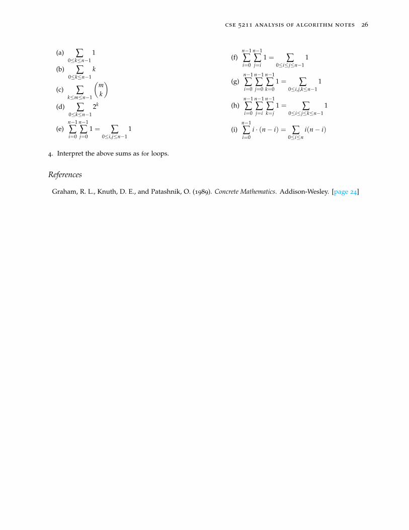
3. Find simple expressions for the following summations.
cse 5211 analysis of algorithm notes 26
(a) ∑0≤k≤n−1
1
(b) ∑0≤k≤n−1
k
(c) ∑k≤m≤n−1
(mk
)(d) ∑
0≤k≤n−12k
(e)n−1
∑i=0
n−1
∑j=0
1 = ∑0≤i,j≤n−1
1
(f)n−1
∑i=0
n−1
∑j=i
1 = ∑0≤i≤j≤n−1
1
(g)n−1
∑i=0
n−1
∑j=0
n−1
∑k=0
1 = ∑0≤i,j,k≤n−1
1
(h)n−1
∑i=0
n−1
∑j=i
n−1
∑k=j
1 = ∑0≤i≤j≤k≤n−1
1
(i)n−1
∑i=0
i · (n− i) = ∑0≤i≤n
i(n− i)
4. Interpret the above sums as for loops.
References
Graham, R. L., Knuth, D. E., and Patashnik, O. (1989). Concrete Mathematics. Addison-Wesley. [page 24]
cse 5211 analysis of algorithm notes 27
More Mathematical Tools
Generating Functions
To analyze algorithms requires skill. Some of these are mathematical. The best math book forcomputer science ever written is 2. 2
Generating functions are a powerful tool for skillfully solving recurrence relations. I recommend thebook (Wilf, 2006) for a deep understanding of generating functions. The idea is that a time complexityfunction T(n) generates a sequence of values ~T = 〈t0, t1, . . .〉 as n ranges over the natural numbers. Thesevalues become coefficients in a formal power series
G(~T, z) =∞
∑k=0
tkzk
Generating functions are discrete analogs of integral transforms from continuous mathematics.There are many functions that generate useful sequences. Here are a few interesting functions.
11− z
=∞
∑n=0
zn 11− 2z
=∞
∑n=0
2nzn
(1− z)−2 =∞
∑n=0
nzn−1 − ln (1− z) =∞
∑n=0
zn+1
n + 1
z(1− z− z2)
=∞
∑n=0
Fnzn (1 + z)m =∞
∑n=0
(mn
)zn
A simple example shows how generating functions can be used to compute the time complexity of analgorithm. Pretend you are given the recurrence relation
T(n) = T(n− 1) + (n− 1), n > 0
corresponding to a code template
1 func t ion ( n ) = funct ion ( n−1) + ( n−1) other operat ions
Now consider the calculation to find the sequence for the function G(z) = ∑∞n=0 tnzn.
G(z) = t0 +∞
∑n=1
tnzn = t0 +∞
∑n=1
[tn−1 + (n− 1)]zn = t0 + z∞
∑n=0
tnzn + z∞
∑n=0
nzn
= t0 + zG(z) +z
(1− z)2
G(z) =t0
1− z+
z(1− z)3 =
∞
∑n=0
t0zn +∞
∑n=0
n(n− 1)2
zn
=∞
∑n=0
[t0 +
(n2
)]zn
T(n) = t0 +
(n2
)
cse 5211 analysis of algorithm notes 28
Complexity Functions
A function f : N 7→N is a proper complexity function (Papadimitriou, 1994) if
1. f is non-decreasing: f (n + 1) ≥ f (n), ∀n
2. There exists a Turing machine M f such that on input x:
(a) M f (x) = t f (|x|) M computes a string of blanks of length f (|x|).(b) M f (x) halts after O(|x|+ f (|x|)) steps
(c) M f (x) uses O(|x|+ f (|x|)) space
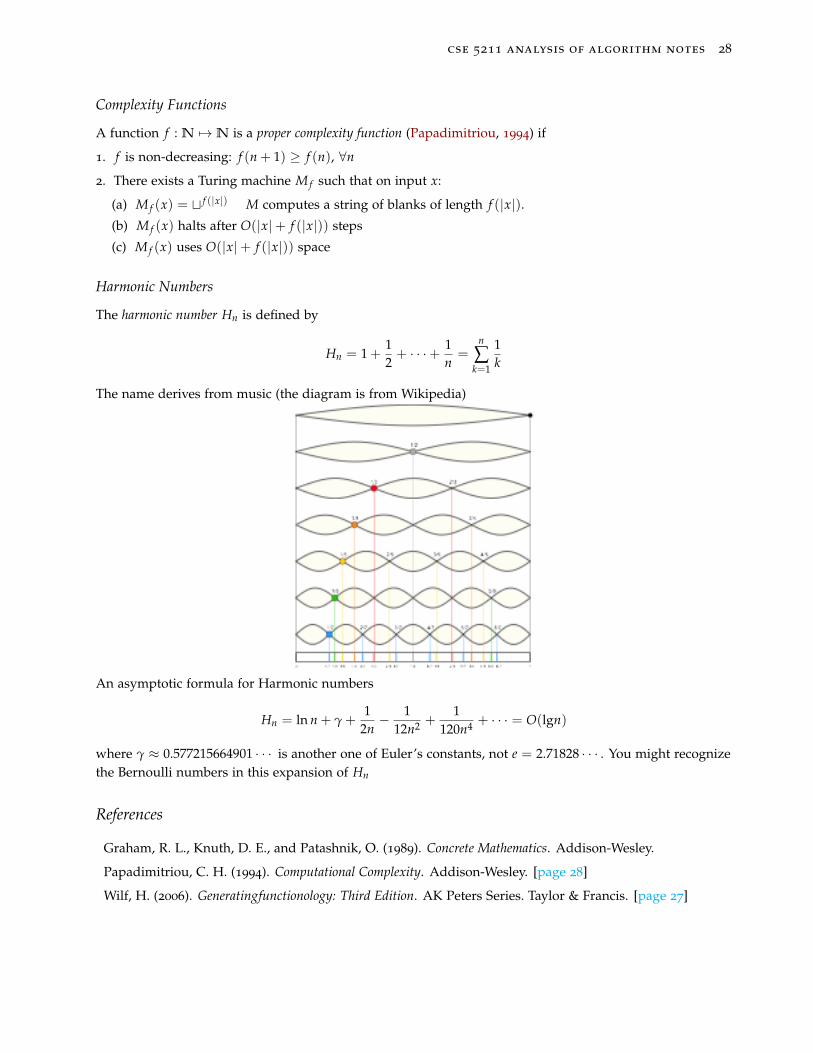
Harmonic Numbers
The harmonic number Hn is defined by
Hn = 1 +12+ · · ·+ 1
n=
n
∑k=1
1k
The name derives from music (the diagram is from Wikipedia)
An asymptotic formula for Harmonic numbers
Hn = ln n + γ +1
2n− 1
12n2 +1
120n4 + · · · = O(lgn)
where γ ≈ 0.577215664901 · · · is another one of Euler’s constants, not e = 2.71828 · · · . You might recognizethe Bernoulli numbers in this expansion of Hn
References
Graham, R. L., Knuth, D. E., and Patashnik, O. (1989). Concrete Mathematics. Addison-Wesley.
Papadimitriou, C. H. (1994). Computational Complexity. Addison-Wesley. [page 28]
Wilf, H. (2006). Generatingfunctionology: Third Edition. AK Peters Series. Taylor & Francis. [page 27]
cse 5211 analysis of algorithm notes 29
Convolutions
Convolve is a function on pairs of sequences. The type of convolve is:
29a 〈Convolve 29a〉≡convolve :: (Num a) => [a] -> [a] -> [a]
Here’s the structure of code to implement the convolve function. The complete code can be found here.
29b 〈Convolution 29b〉≡module Convolution ( convolve ) where
〈Auxiliary functions 29c〉〈Convolve 29a〉〈Main module 32b〉
Motivation
The modern impetus for convolutions comes from signal processing: An input signal [as] is convolved withan impulse-response signal [bs] to produce a third signal, the convolution [cs] of [as] and [bs]. Signalprocessing is beyond the scope of this course (can you supply some classic references?)
The discovery of convolutions must have come from polynomial multiplication. Consider these smallpolynomial products.
(a0 + a1z)(b0 + b1z) = [a0b0] + [a0b1 + a1b0]z + [a1b1]z2
(a0 + a1z + a2z2)(b0 + b1z + b2z2) = [a0b0] + [a0b1 + a1b0]z + [a0b2 + a1b1 + a2b0]z2 + [a1b2 + a2b1]z3 + [a2b2]z4
Notice the pattern: Each coefficient in the product is an inner product of coefficients from [as] and [bs].Tangentially, recall, an inner or dot product of lists [xs] and [ys] is define as
〈 xs | ys | = 〉 ∑0≤k
xkyk
And can be implemented by the code:
29c 〈Auxiliary functions 29c〉≡〈Inner Product 29d〉
29d 〈Inner Product 29d〉≡ip :: Num a => [a] -> [a] -> a
ip [] ys = 0
ip xs [] = 0
ip (x:xs) (y:ys) = x*y + ip xs ys
cse 5211 analysis of algorithm notes 30
What is the time complexityof ip?What is the time complexityof ip?And now, back to the story. The coefficients in the product are, in order of powers, are:
〈 [a0] | [b0] | 〉 = a0b0
〈 [a0, a1] | [b1, b0] | 〉 = a0b1 + a1b0
〈 [a0, a1, a2] | [b2, b1, b0] | 〉 = a0b2 + a1b1 + a2b0
In general the products of polynomials with degrees n and m is(∑
0≤j≤najzj
)·(
∑0≤j≤m
bjzj
)= ∑
0≤i≤n+m
(∑
0≤k≤iakbi−k
)zi
The indices can be out-of-bounds for some instances. For instance when n = 1 and m = 2, the formula forthe coefficient of z3 would be [a2b1 + a1b2], but a2 is undefined. Consider,
(a0 + a1z)(b0 + b1z + b2z2) = [a0b0] + [a0b1 + a1b0]z + [a0b2 + a1b1]z2 + [a1b2]z3
In this case, a2 is undefined, so it is convenient to set a2 = 0 so the quadratic and cubic coefficients can bewritten as [a0b2 + a1b1 + a2b0] and [a1b2 + a2b1] respectively. In the opposite case, when n > m the productis
(a0 + a1z + a2z2)(b0 + b1z) = [a0b0] + [a0b1 + a1b0]z + [a1b1 + a2b0]z2 + [a2b1]z3
In this case, b2 is undefined, and setting b2 = 0 allows quadratic and cubic coefficients to be written as[a0b2 + a1b1 + a2b0] and [a1b2 + a2b1] respectively. In this way, it is best to define this problem away.
Algorithm Implementation
The lists [as] and [bs] can be padded with 0’s to have equal lengths eliminating this problem.
30a 〈Auxiliary functions 29c〉+≡〈Pad 30b〉
Given two lists xs and ys, the pad function puts 0’s in in front of xs, where the number of 0’s is 1 lessthan the length of ys.
30b 〈Pad 30b〉≡pad :: [a] -> [a] -> [a]
pad xs ys = (replicate ((length ys) - 1) 0) ++ xs

cse 5211 analysis of algorithm notes 31
Another important observation is: In the coefficient calculation, [as] occur in order while the [bs] isreversed.
Let’s work through an instance of convolve to see what must be done. Let as= [1, 2, 3] and bs=
[4, 5, 6, 7].First, pad as with 3 zeros and bs with 2:
padas = [0, 0, 0, 1, 2, 3] and padbs = [0, 0, 4, 5, 6, 7]
Reverse padbs, the last list:[0, 0, 0, 1, 2, 3] and [7, 6, 5, 4, 0, 0]
And take inner products of tails and heads of the two lists:
〈 [0, 0, 0, 1, 2, 3] | [7, 6, 5, 4, 0, 0] | = 〉4〈 [0, 0, 1, 2, 3] | [7, 6, 5, 4, 0 | = 〉13
〈 [0, 1, 2, 3] | [7, 6, 5, 4 | = 〉28
〈 [1, 2, 3] | [7, 6, 5 | = 〉34
〈 [2, 3] | [7, 6] | = 〉32
〈 [3] | [7] | = 〉21
The function tails, from the Data.List module, maps a list to its tails, e.g., tails [1, 2, 3] = [[1, 2,
3], [2, 3], [3], []]. Composing this with the init function removes the last empty list []. Strangely, Ithink, there is no function heads in Data.List It would act like this: heads [7, 6, 5] = [[7, 6, 5], [7,
6], [7]]. But, heads can be defined.
31a 〈Auxiliary functions 29c〉+≡〈Heads 31b〉The list of heads is the cons of the list with the heads of the list without the last term (init heads).
31b 〈Heads 31b〉≡heads :: [a] -> [[a]]
heads [x] = [[x]]
heads xs = xs : heads (init xs)
cse 5211 analysis of algorithm notes 32
Putting it all together
So here’s what must be done to complete convolve.
• Define convolve’s initial values when one list is empty.
• Pad the two signals so they have the same length.
• Zip inner products across the tails of the padded [as] with the heads of the reverse of the padded[bs].
32a 〈Convolve 29a〉+≡convolve _ [] = []
convolve [] _ = []
convolve as bs =
let padas = pad as bs
padbs = pad bs as
in zipWith (ip) (init $ tails padas) (heads $ reverse padbs)
32b 〈Main module 32b〉≡- To compile an executable, a [[main]] function is needed for input and output.
- I don’t want to think about this right now .
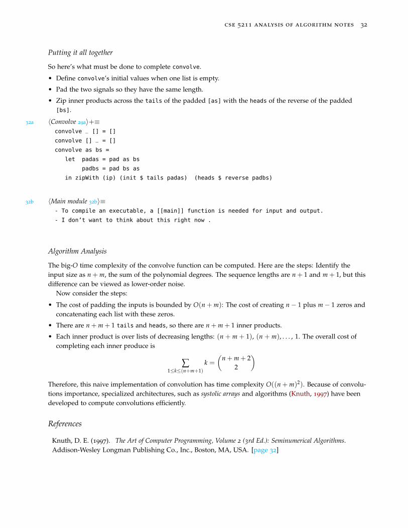
Algorithm Analysis
The big-O time complexity of the convolve function can be computed. Here are the steps: Identify theinput size as n + m, the sum of the polynomial degrees. The sequence lengths are n + 1 and m + 1, but thisdifference can be viewed as lower-order noise.
Now consider the steps:
• The cost of padding the inputs is bounded by O(n + m): The cost of creating n− 1 plus m− 1 zeros andconcatenating each list with these zeros.
• There are n + m + 1 tails and heads, so there are n + m + 1 inner products.
• Each inner product is over lists of decreasing lengths: (n + m + 1), (n + m), . . . , 1. The overall cost ofcompleting each inner produce is
∑1≤k≤(n+m+1)
k =
(n + m + 2
2
)
Therefore, this naive implementation of convolution has time complexity O((n + m)2). Because of convolu-tions importance, specialized architectures, such as systolic arrays and algorithms (Knuth, 1997) have beendeveloped to compute convolutions efficiently.
References
Knuth, D. E. (1997). The Art of Computer Programming, Volume 2 (3rd Ed.): Seminumerical Algorithms.Addison-Wesley Longman Publishing Co., Inc., Boston, MA, USA. [page 32]
cse 5211 analysis of algorithm notes 33
Representative Problems
The idea here is to consider a sequence of problems that resemble one another, but have increasing levelsof difficulty. The outline is based on chapter 1 of (Kleinberg and Tardos, 2006).
Interval Scheduling
Scheduling Compatible Intervals (JS): A set J of n (potentially overlapping) intervals (jobs) over a period oftime. Each job k has start and finish times sk < fk and duration fk − sk > 0. Two jobs i and j are compatibleif they do not overlap: fi ≤ sj or f j ≤ si (job i finish at or before the start of job j, and vice versa.) Jobcompatible is an irreflexive symmetric relation.
The maximum job compatiblity problem (MJCP) is to find a subset of mutually compatible jobs that hasthe largest duration: sum of lengths.
max
∑A
( fk − sk) : k ∈ A, where A is a set of mutually compatible intervals
Exercise 1: How would you find this maximum values?
Exercise: 2 Is it reasonable to form all subsets of the n jobs and check: Are the jobs jobs compatible? Howmany subsets of n jobs are there? How many comparisons would be needed (in the worst case) to showthat a subset of k jobs is compatible? How much effort would be needed to keep track of the subset with alongest duration?
This brute-force algorithm: Search over all subsets of jobs to find one that is compatible and has thelongest duration shows the JS problem in computable (there is a effective method to solve the problem). But,this brute-force approach has high complexity: There are (n
k) subsets of size k and k(k− 1)/2 comparisonsare needed to show a subset of jobs is compatible. How big can (n
k) be?Here’s a greedy heuristic, that can be visualized as a matching problem. Pretend the jobs have been sorted
by earliest finishing time.(∀ k)( fk ≤ fk+1)
Draw two horizonal time-lines: The one for starts and a second for finishes. Plot some start times on thetop line and some later finishing times on the bottom line; connect them with dotted lines. How can com-patible intervals be identified?
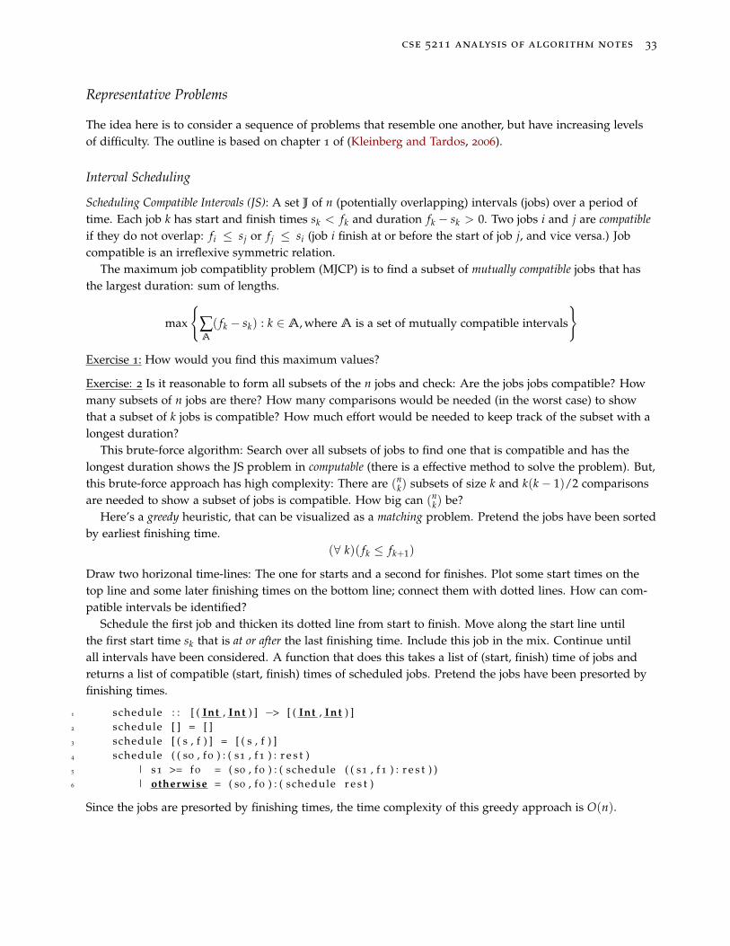
Schedule the first job and thicken its dotted line from start to finish. Move along the start line untilthe first start time sk that is at or after the last finishing time. Include this job in the mix. Continue untilall intervals have been considered. A function that does this takes a list of (start, finish) time of jobs andreturns a list of compatible (start, finish) times of scheduled jobs. Pretend the jobs have been presorted byfinishing times.
1 schedule : : [ ( Int , Int ) ] −> [ ( Int , Int ) ]2 schedule [ ] = [ ]3 schedule [ ( s , f ) ] = [ ( s , f ) ]4 schedule ( ( s0 , f0 ) : ( s1 , f1 ) : r e s t )5 | s1 >= f0 = ( s0 , f0 ) : ( schedule ( ( s1 , f1 ) : r e s t ) )6 | otherwise = ( s0 , f0 ) : ( schedule r e s t )
Since the jobs are presorted by finishing times, the time complexity of this greedy approach is O(n).

cse 5211 analysis of algorithm notes 34
The function schedule does not compute the maximum duration. To do that, a function that take theoutput of schedule and sums the duration of each interval is needed.
Weighted interval scheduling
Now pretend each job k has an associated value vk. Imagine the edges in the start-finish graph as havingweights representing the job’s value.
max
∑A
vk : k ∈ A, where A is a set of mutually compatible intervals
Greedy approaches do not succeed for this variation of the problem. (An early to finish job may have littlevalue, while high value non-compatibles job are not chosen.) A dynamic programming approach where op-timal solutions are memoized for each increasing subset of jobs: 0, 1, . . . , k can produce an optimal solution.As each new job is considered, the new optimal value is the largest of the previous set of jobs or the valueof the new job plus the value of the optimal subset of jobs compatible with the new job.
Define p(k), for an job k, to be the largest index i < k such that intervals i and k are disjoint. Definep(k) = 0 if no request i < k is disjoint from k.
v0 = 2, p(0) = 0
v1 = 4, p(1) = 0
v2 = 4, p(2) = 1
v3 = 7, p(3) = 0
v4 = 2, p(4) = 3
v5 = 1, p(5) = 3
A top-down recursive algorithms in pseudo-code is:
1 computeOpt ( i n t k , i n t * v ) 2 i f ( k == 0 ) return v [ 0 ] ; 3 e lse return max ( CcmputeOpt ( k−1 , v ) , v [ k ] + computeOpt ( p ( k ) , v ) ;4
A bad instance occurs when p(k) = k− 2 for all k. In this case, computeOpt makes a Fibonacci-like sequenceof calls and the algorithm executes in exponential time in the worst case.
Computing and storing the optimal values bottom-up for look-up when needed is the dynamic program-ming idea. Assume these optimal values are stored in an array m[0..n], where m[k] holds the value Assumem[k] is set to −1 initially.
1 memoizedComputeOpt ( i n t k , i n t * v ) 2 i f ( k == 0 ) return 0 ; 3 e lse i f (m[ k ] != −1) return m[ k ] ; 4 e lse m[ k ] = max ( v [ k]+m[ p [ k ] ] , m[ k−1 ] ) ; return m[ k ] ;

cse 5211 analysis of algorithm notes 35
Bipartite matching
Given a graph G = (V, E) can its vertices V be partitions into disjoint sets X and Y such that each edgesstarts in X and ends in Y?
A matching is a subset of edge M ⊆ E such that no two edges in M share a common vertex. Each vertexv ∈ V is in at most one edge in M. Some vertices may not be on any edge in M. A perfect matching is amatching M ⊆ E such each vertex v ∈ V is in exactly one edge in M. That is, every vertex of the graph isincident to exactly one edge of the matching.
The bipartite matching problem (BMP) is: Give a bipartite graph G, find a matching of maximum size. If|X| = |Y| = n, then a perfect matching is a maximal matching and its size is n.
Greedy and dynamic programming approaches do not appear to work for bipartite matching. The prob-lem can be reduced to a network flow problem by adding a source s and a sink t node. A backtracking ap-proach leads to an efficient solution.
s t
Independent Set
In a graph G = (V, E) a set I of vertices is independent if no two vertices in I are adjacent (there is no edgeconnecting any pair of vertices in I).
A function problem is to find a maximal independent set. The graph below shows an independent set(the black nodes) of size 6.
Finding the maximal independent set is an NP-hard optimization problem. A non-deterministic polynomial-time hard problem P is one such that every NP problem Q can be reduced to P in polynomial time. As aconsequence, finding a polynomial algorithm to solve any NP-hard problem would give polynomial algo-rithms for all the problems in NP, which is unlikely as many of them are considered hard.

cse 5211 analysis of algorithm notes 36
References
Kleinberg, J. and Tardos, E. (2006). Algorithm Design. Pearson. [page 33]

cse 5211 analysis of algorithm notes 37
Binomial Coefficients
Pascal’s Triangle: Divide-and-Conquer
Consider computing binomial coefficients. There are multiple methogs. The recursive Pascal’sidentity is perhaps the most common. (
nk
)=
(n− 1
k
)+
(n− 1k− 1
)with boundary conditions (
n0
)=
(nn
)= 1
The recursion tree shows multiple overlapping sub-problems, which is a clear sign that direct recursionwill more costly than necessary. At each level the values of the left and right nodes are added: There is oneadd at level 1, two adds at level 2, four adds at level 3, six adds at level 4, and six adds at level 5. A total of19 additions.
(63)
(53)
(43)
(33) (3
2)
(22) (2
1)
(11) (1
0)
(42)
(32)
(22) (2
1)
(11) (1
0)
(31)
(21)
(11) (1
0)
(20)
(52)
(42)
(32)
(22) (2
1)
(11) (1
0)
(31)
(21)
(11) (1
0)
(20)
(41)
(31)
(21)
(11) (1
0)
(20)
(30)
The factorial expressionn!
k!(n− k)!
solves the equation and boundary conditions, so it must be big-O time time complexity of an algorithmthat implements this recurrence. Indeed (6
3) = 20 and 19 additions were counted (there are 19 additionsamong 20 terms). A recursion stack depth of size n must also be maintained.
Binomial coefficients attain their maximum at the median of each row. In even rows this is
2n!n!n!
, n = 0, 2, 3, . . .
In odd rows there are two maxima.
(2n + 1)!n!(n + 1)!
=(2n + 1)!(n + 1)!n!
, n = 1, 2, 3, . . .
Stirling’s asymptotic approximation
n! ∼√
2πn(n
e
)n
cse 5211 analysis of algorithm notes 38
can be used to approximate the factorial expression for binomial coefficients.
(2n)!n!n!
∼√
2π2n( 2n
e)2n
(√
2πn( n
e)n)2
=2n√
πn
Pascal’s Triangle: Dynamic Programming
Precompute, don’t recompute! The dictum of dynamic programming. Each binomial coefficientis computed once, from the bottom up and stored in a table. Given n and k, do this to compute (n
k):
1. Initialize the boundaries: The left and right boundaries are fixed at 1.
2. For each row i = 0 to n and for each column j = 0 to k compute and store (ij)
1 f o r ( i n t i = 0 ; i <= n ; i ++) bc [ i ] [ 0 ] = 1 ; bc [ i ] [ i ] = 1 ; 2 f o r ( i n t i = 0 ; i <= k ; i ++) 3 f o r ( i n t j = 1 ; i <= k ; i ++) 4 bc [ i ] [ j ] = bc [ i −1][ j ] + bc [ i −1][ j −1] ;5 6
Using simple translations of for loops into summations, the time complexity is
k
∑i=1
i
∑j=1
c +n
∑i=k+1
k
∑j=1
c =k
∑i=1
ic +n
∑i=k+1
kc = c(
k + 12
)+ ck(n− k) ≤ n(n + 2)
4+
n2
4
This captures a main concept of dynamic programming, use of a table to store values, but it misses animportant aspect: Neither a minimum or maximum is required over a set of previously computed values.
The Factorial Algorithm
The factorial expression could be evaluated directly. Computing n!/k!(n− k)! takes n − 1multiplies for the numerator and (k− 1) + (n− k− 1) + 1 = n− 1 multiplies for the denominator plus onedivision. However, integer overflow is a concern. Assuming a 64 bit register for naturals, the largest valuethat can be stored is 264 − 1 = 18, 446, 744, 073, 709, 551, 616− 1. But at 21! = 51, 090, 942, 171, 709, 440, 000overflow will occur.
The Absorption Identity
It is easy to verify the absorption identity for binomial coefficients.(nk
)=
nk
(n− 1k− 1
),(
n− k0
)= 1,
(n− k + 1
1
)= n− k + 1
This leads to a linear recursion tree. For instance,(63
)=
63
(52
)=
63· 5
2
(41
)=
63· 5
2· 4

cse 5211 analysis of algorithm notes 39
It may be best to refactor the computation to avoid any complications between integer and floating pointarithmetic. (
63
)= 6
(52
)/3 = 6(5
(41
)/2)/3 = (6 · 5)(4)/2)/3
This approach executes k − 1 multiplies and k − 1 divides. And, when unrolled like this, the algorithmbecomes a product method for computing (n
k). Here’s Haskell code for this computation.
1 choose : : ( I n t e g r a l a ) => a −> a −> a2 choose n k = product [ k + 1 . . n ] ‘ div ‘ product [ 2 . . n−k ]

cse 5211 analysis of algorithm notes 40
Divide and Conquer
Divide-and-rule is attributed to Phillip of Macedonia, father of Alexander the Great. Inpolitics and warfare the phrase describes a strategy to separate adversaries into smaller and smaller groupsuntil each can be readily defeated. In computer science, divide-and-conquer summarizes a problem solvingparadigm. Unlike warfare, where the objective is destruction, divide-and-conquer problem solving requiresrebuilding an overall solution from solutions to sub-problems. There are several classic divide-and-conqueralgorithms.
Euclidean Algorithm
The Euclidean algorithm is literally divide-and conquer. It computes the largest common divisorof two integers, not both 0.
gcd(a, 0) = a
gcd(a, m) = gcd(m, a mod m), for m > 0
In C, the code might look something like this:
1 i n t gcd ( i n t a , i n t m) 2 i n t t ;3 while (m) 4 t = a ; a = m; m = t % a ;5 6 return a < 0 ? −a : a ;7
Here’s a functional implementation from Haskell’s standard Prelude.
1 gcd : : ( I n t e g r a l a ) => a −> a −> a2 gcd 0 0 = e r r o r "Prelude.gcd: gcd 0 0 is undefined"
3 gcd x y = gcd ’ ( abs x ) ( abs y ) where4 gcd ’ a 0 = a5 gcd ’ a m = gcd ’ m ( a ‘rem ‘ m)
Analysis of the Euclidean algorithm is the subject of a student presentation. The upshot is that Fibonacci-like sequences produce the worst case time behavior. The time complexity grows like the log base ϕ ≈1.618 of max |x| , |y|. The gcd algorithm is very efficient.
Merge Sort
Consider the well-known mergeSort algorithm. The cost depends on splitting a list into two parts.
1 s p l i t ( x : y : zs ) = l e t ( xs , ys ) = s p l i t zs in ( x : xs , y : ys )2 s p l i t [ x ] = ( [ x ] , [ ] )3 s p l i t [ ] = ( [ ] , [ ] )
cse 5211 analysis of algorithm notes 41
This splitting is not stable, but is reasonable efficient on lists. It places every other item on one of two lists.The recurrence that describes split ’s time complexity is
Tsplit(n) = Tsplit(n− 2) + c, Tsplit(n) =nc2
= O(n)
The split lists will have the same size or the first will be one more than the secondOnce split, the two lists need to be merged into one.
1 merge [ ] ys = ys2 merge xs [ ] = xs3 merge xs@ ( x : x t ) ys@ ( y : yt ) | x <= y = x : merge xt ys4 | otherwise = y : merge xs yt
The recurrence that describes merge’s time complexity is
Tmerge(n) = Tmerge(n− 1) + b, Tmerge(n) = nb = O(n)
To complete the sort, split the lists, mergeSort both halves, and merge the results.
1 mergeSort [ ] = [ ]2 mergeSort [ x ] = [ x ]3 mergeSort xs = l e t ( as , bs ) = s p l i t xs4 in merge ( mergeSort as ) ( mergeSort bs )
The recurrence that describes mergeSort’s time complexity is
TmergeSort(n) = Tsplit(n) + 2TmergeSort(n/2) + Tmerge(n)
Or, more simplyTmergeSort(n) = 2TmergeSort(n/2) + O(n)
which as solutionTmergeSort(n) = O(n lg n)
Binary Search
Binary search is a classic algorithm. Given a ordered list xs, a value to search for, and a range fromlow to high over which to search, binsearch returns the position (index) where value is found, or Nothing if itis not in the list. The cases are:
• Nothing when the range is empty
• The result of searching the bottom half of the range when value is smaller than the value in the middleof the range
• The result of searching the top half of the range when value is larger than the value in the middle of therange
• And, Just mid, the middle value when it equals value.
cse 5211 analysis of algorithm notes 42
1 binsearch : : [ Int ] −> Int −> Int −> Int −> Maybe Int2 binsearch xs value low high3 | high < low = Maybe Nothing4 | xs ! ! mid > value = binsearch xs value low ( mid−1)5 | xs ! ! mid < value = binsearch xs value ( mid+1) high6 | otherwise = Jus t mid7 where8 mid = low + ( ( high − low ) ‘ div ‘ 2 )
Working with lists instead of arrays increased the running time of the algorithm. There is a cost of orderO(n/2) to walk through the list to its middle. The time complexity recurrence for the list-based algorithmis
T(n) = T(n/2) + cn, n = 2k, k = 1, 2, . . . , T(1) = 1
where n is the length of the list x.
T(n) = T(n/2) + cn
= [T(n/4) + cn/2] + cn
= [T(n/8) + cn/4] + cn/2 + cn
=...
= T(n/2k) + cn/2k−1 + · · ·+ cn/4 + cn/2 + cn
= T(1) + cn ∑0≤j<k
(1/2)j
= 1 + cn(
2− 2n
)= 2cn + 1− 2c = O(n)
The array-based algorithm has constant time access to values by index. And, in this case, the recurrence is
T(n) = T(n/2) + c, n = 2k, k = 1, 2, . . . , T(1) = 1
Show T(n) = O(lg n) for theequation T(n) = T(n/2) + c.Show T(n) = O(lg n) for theequation T(n) = T(n/2) + c.
cse 5211 analysis of algorithm notes 43
The Quicksort Algorithm
The quicksort algorithm is attributed to Tony Hoare (Hoare, 1961). Sedgewick’s analysis of quicksort(Sedgewick, 1977) and (Sedgewick, 1978) provide an in-depth analysis and details of its implementation.The basic idea is to place the head of a list in its correct position with smaller elements before it and largerelements after it. The head is often called the pivot.
1 qsor t : : Ord a => [ a ] −> [ a ]2 qsor t [ ] = [ ]3 qsor t ( p : xs ) = qsor t [ x|x<−xs , x<p ] ++ [ p ] ++ qsor t [ x|x<−xs , x>=p ]
Here imperative code for quick sorting (Bentley, 1984). Assume a sentinel at A[0] that keeps indices withinbounds.
1 void quickSort ( i n t A[ ] , i n t lo , i n t hi ) 2 i n t pivot ;3 i f ( hi > lo ) 4 pivot = p a r t i t i o n (A, lo , hi ) ;5 quickSort (A, lo , pivot −1) ;6 quickSort (A, pivot +1 , h i ) ;7 8 9 i n t p a r t i t i o n ( i n t A[ ] , i n t lo , i n t hi )
10 11 i n t i , j , p ;12 i = lo − 1 ; j = hi ; p = A[ j ] ;13 f o r ( ; ; ) 14 while (A[++ i ] < p ) ;15 while (A[−− j ] > p ) ;16 i f ( i >= j ) break ;17 swap (A[ i ] , A[ j ] ) ;18 19 swap (A[ i ] , A[ hi ] ) ;20 return i ;21
position 1 2 3 4 5 6 7 8 9
array 3 9 12 15 11 17 6 8 14
pivot p
indexes i j
swap 8 15
indexes i j
swap 6 17
indexes j i
swap 3 9 12 8 11 6 14 15 17
Let’s analyze quicksort.
cse 5211 analysis of algorithm notes 44
Given an array of length n, quicksort makes two calls to itself, once with an array of length p and oncewith an array of length n− p− 1. Here p is the size of the array from lo to pivot-1 The cost of the call topartition is n + 1 = O(n).
In the worst case p = 0 andT(n) = (n + 1) + T(n− 1)
with initial condition T(1) = 1. By mathematical induction, or unrolling the recurrence, or telescopingsums
T(n) = (n + 1) + (n) + (n− 1) + · · ·+ 3 + T(1)
= (n + 1) + (n) + (n− 1) + · · ·+ 3 + (2 + 1− 2)
= (n + 1)(n + 2)/2− 2
= O(n2)
In the best case, the pivot is p = n/2 and partitions the array into sub-arrays of equal size. The recur-rence relation is
T(n) = (n + 1) + 2T(n/2)
We are cheating a little here since n − p − 1 = n/2 − 1 6= n/2, but this fudge will not alter the timinganalysis.
Unrolling the formula
T(n) = (n + 1) + 2(n/2 + 1) + · · ·+ 2qT(n/2q)
= n lg n + 2n− 1
= O(n lg n)
where n = 2q is a power of 2 and q = lg n.
References
Bentley, J. (1984). Programming Pearls: How to sort. Commun. ACM, 27(4):287–ff. [page 43]
Hoare, C. A. R. (1961). Quicksort. Computer Journal, 5(1):10–15. [page 43]
Sedgewick, R. (1977). The analysis of quicksort programs. Acta Informatica, 7:327–355. [page 43]
Sedgewick, R. (1978). Implementing quicksort programs. Communications of the ACM, 21(10):847–857.[page 43]
cse 5211 analysis of algorithm notes 45
Quicksort
Quicksort (Hoare, 1961) is a classic algorithm that has a nice description in Haskell. The outline for theQuicksort module is simple: Import other needed modules, define functions as needed, and include a main
function for IO and testing.
45a 〈Quicksort 45a〉≡module Quicksort ( quicksort ) where
〈Import external modules 46a〉〈Auxiliary functions 45b〉〈Main function 46c〉The quicksort function sorts a list of values into increasing order. The idea is simple. Given a list
(p:xs) with pivot p at its head:
1. Walk over the list and place all values x in the tail xs that are less than p in a list.
2. Quicksort this list.
3. Concatenate the sorted list with [p].
4. Walk over the original list again and place all values x in the tail xs that are greater than or equal to p inanother list.
5. Quicksort this list.
6. Concatenate this sorted list with the list from step 3.
Here’s the code.
45b 〈Auxiliary functions 45b〉≡quicksort :: Ord a => [a] -> [a]
quicksort [] = []
quicksort (p:xs) = quicksort [x| x<-xs, x < p] ++ [p] ++ quicksort [x | x<-xs, x >= p]
Quicksort Analysis
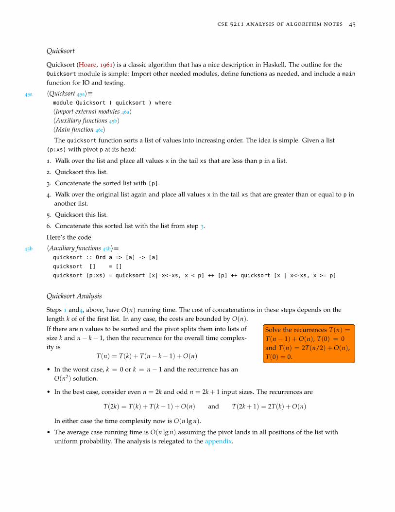
Steps 1 and4, above, have O(n) running time. The cost of concatenations in these steps depends on thelength k of of the first list. In any case, the costs are bounded by O(n).
If there are n values to be sorted and the pivot splits them into lists of Solve the recurrences T(n) =T(n − 1) + O(n), T(0) = 0and T(n) = 2T(n/2) + O(n),T(0) = 0.
Solve the recurrences T(n) =T(n − 1) + O(n), T(0) = 0and T(n) = 2T(n/2) + O(n),T(0) = 0.
size k and n− k− 1, then the recurrence for the overall time complex-ity is
T(n) = T(k) + T(n− k− 1) + O(n)
• In the worst case, k = 0 or k = n − 1 and the recurrence has anO(n2) solution.
• In the best case, consider even n = 2k and odd n = 2k + 1 input sizes. The recurrences are
T(2k) = T(k) + T(k− 1) + O(n) and T(2k + 1) = 2T(k) + O(n)
In either case the time complexity now is O(n lg n).
• The average case running time is O(n lg n) assuming the pivot lands in all positions of the list withuniform probability. The analysis is relegated to the appendix.

cse 5211 analysis of algorithm notes 46
Testing Quicksort
To test the code, generate some random sequences. Use ghci to unit testcreateList and quicksort.Compile the code with profil-ing options, collect run timedata and compare your ex-periment with theory.
Use ghci to unit testcreateList and quicksort.Compile the code with profil-ing options, collect run timedata and compare your ex-periment with theory.
46a 〈Import external modules 46a〉≡import System.Random
And, create a list of n random integers with createList n.
46b 〈Auxiliary functions 45b〉+≡createList :: Int -> [Int]
createList n = take n (randoms (mkStdGen 10))
The main routine can then read an integer, create a list, sort it, and show the results.
46c 〈Main function 46c〉≡main :: IO ()
main = interact (show . quicksort . createList . read)
cse 5211 analysis of algorithm notes 47
Appendix: An average case analysis of quicksort
The expression for average case running time is
Tave(n) = ∑all cases
Pr(case)T(case) + (n + 1)
Write the Quicksort recurrence as
T(n) = T(k) + T(n− k− 1) + (n + 1), n > 0, and T(0) = 1
Let’s assume, with uniform probability Pr(case) = 1/n, that the pivot partitions the length n list intotwo lists: One of length k and another of length n− k − 1, for k = 0, . . . , n− 1. This give the average caseexpression for Quicksort at
T(n) = (n + 1) +1n ∑
0≤k<n[T(k) + T(n− k− 1)]
= (n + 1) +1n
[∑
0≤k<nT(k) + ∑
0≤k<nT(n− k− 1)
]
= (n + 1) +1n
[∑
0≤k<nT(k) + ∑
0≤k<nT(k)
]
= (n + 1) +2n ∑
0≤k<nT(k)
Now, massage T(n) into shape.
• Remove the fraction by multiplying by n giving
nT(n) = n(n + 1) + 2 ∑0≤k<n
T(k)
• Remove the sum by substituting n + 1 for n, and subtract the two expressions
(n + 1)T(n + 1)− nT(n) =
[(n + 1)(n + 2) + 2 ∑
0≤k<n+1T(k)
]−[
n(n + 1) + 2 ∑0≤k<n
T(k)
]= 2(n + 1) + 2T(n)
Next, define the generating function G(z) for the sequence 〈T0, T1, . . .〉.
G(z) = T0 + T1z + T2z2 + T3z3 + · · ·= ∑
0≤kTkzk
cse 5211 analysis of algorithm notes 48
And notice
G′(z)− zG′(z) = ∑0≤k
kTkzk−1 − z ∑0≤k
kTkzk−1
(1− z)G′(z) = ∑0≤k
(k + 1)Tk+1zk − ∑0≤k
kTkzk
= ∑0≤k
[(k + 1)Tk+1 − kTk] zk
= ∑0≤k
[2(k + 1) + 2Tk] zk
=2
(1− z)2 + 2G(z)
Multiply by (1− z) and rearrange terms to get a perfect differential.
(1− z)2G′(z)− 2(1− z)G(z) =2
1− z
that isddz
(1− z)2G(z) = (1− z)2G′(z)− 2(1− z)G(z) =2
1− zIntegrating both sides gives
(1− z)2G(z) = −2 ln(1− z) + C
where C = 0 since G(0) = T0 = 0 So we have
G(z) =−2
(1− z)2 (ln(1− z)
The Cauchy product of two power series is(∑0≤i
aixi
)·(
∑0≤j
bjxj
)= ∑
0≤ncnxn
wherecn = ∑
0≤k≤nan−kbk
It follows that
G(z) =−2
(1− z)2 · ln(1− z)
= 2 ∑1≤i
(i + 1)zk ·∑1≤j
zj
j
= 2 ∑1≤n
[∑
1≤k≤n
n + 1− kk
]zn
= ∑1≤n
∑1≤k≤n
[2(n + 1)
k− 2]
zn
= ∑1≤n
[2(n + 1)Hn − 2n]zn

cse 5211 analysis of algorithm notes 49
Recall the Harmonic numbers
Hn = ∑1≤k≤n
1k= 1 +
12+
13+
14+ · · ·+ 1
n
= Hn−1 +1n
n ≥ 1
H0 = 0
The harmonic number Hn can be asymptotically approximated by
Hn ∼ ln n + γ + O(1/2n)
where γ ≈ 0.5772156649 · · · is Euler’s constant.Therefore, the average case time complexity of Quicksort is
T(n) = 2(n + 1)Hn − 2n = O(n lg n)
References
Hoare, C. A. R. (1961). Quicksort. Computer Journal, 5(1):10–15. [page 45]
Sedgewick, R. (1977). The analysis of quicksort programs. Acta Informatica, 7:327–355.
Sedgewick, R. (1978). Implementing quicksort programs. Communications of the ACM, 21(10):847–857.
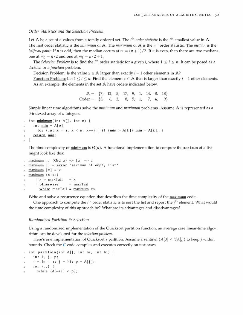
cse 5211 analysis of algorithm notes 50
Order Statistics and the Selection Problem
Let A be a set of n values from a totally ordered set. The ith order statistic is the ith smallest value in A.The first order statistic is the minimum of A. The maximum of A is the nth order statistic. The median is thehalfway point: If n is odd, then the median occurs at m = (n + 1)/2. If n is even, then there are two mediansone at m0 = n/2 and one at m1 = n/2 + 1.
The Selection Problem is to find the ith order statistic for a given i, where 1 ≤ i ≤ n. It can be posed as adecision or a function problem.
Decision Problem: Is the value x ∈ A larger than exactly i− 1 other elements in A?Function Problem: Let 1 ≤ i ≤ n. Find the element x ∈ A that is larger than exactly i− 1 other elements.As an example, the elements in the set A have orders indicated below.
A = 7, 12, 5, 17, 9, 1, 14, 8, 18Order = 3, 6, 2, 8, 5, 1, 7, 4, 9
Simple linear time algorithms solve the minimum and maximum problems. Assume A is represented as a0-indexed array of n integers.
1 i n t minimum( i n t A[ ] , i n t n ) 2 i n t min = A[ 0 ] ;3 f o r ( i n t k = 1 ; k < n ; k++) i f ( min > A[ k ] ) min = A[ k ] ; 4 return min ;5
The time complexity of minimum is Θ(n). A functional implementation to compute the maximum of a listmight look like this:
1 maximum : : ( Ord a ) => [ a ] −> a2 maximum [ ] = e r r o r "maximum of empty list"
3 maximum [ x ] = x4 maximum ( x : xs )5 | x > maxTail = x6 | otherwise = maxTail7 where maxTail = maximum xs
Write and solve a recurrence equation that describes the time complexity of the maximum code.One approach to compute the ith order statistic is to sort the list and report the ith element. What would
the time complexity of this approach be? What are its advantages and disadvantages?
Randomized Partition & Selection
Using a randomized implementation of the Quicksort partition function, an average case linear-time algo-rithm can be developed for the selection problem.
Here’s one implementation of Quicksort’s partition. Assume a sentinel (A[0] ≤ ∀A[j]) to keep j withinbounds. Check the C code compiles and executes correctly on test cases.
1 i n t p a r t i t i o n ( i n t A[ ] , i n t lo , i n t hi ) 2 i n t i , j , p ;3 i = lo − 1 ; j = hi ; p = A[ j ] ;4 f o r ( ; ; ) 5 while (A[++ i ] < p ) ;
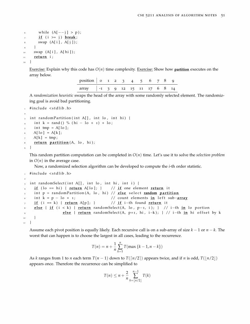
cse 5211 analysis of algorithm notes 51
6 while (A[−− j ] > p ) ;7 i f ( i >= j ) break ;8 swap (A[ i ] , A[ j ] ) ;9
10 swap (A[ i ] , A[ hi ] ) ;11 return i ;12
Exercise: Explain why this code has O(n) time complexity. Exercise: Show how partition executes on thearray below.
position 0 1 2 3 4 5 6 7 8 9
array -1 3 9 12 15 11 17 6 8 14
A randomization heuristic swaps the head of the array with some randomly selected element. The randomiz-ing goal is avoid bad partitioning.
1 # include < s t d l i b . h>2
3 i n t randomPartit ion ( i n t A[ ] , i n t lo , i n t hi ) 4 i n t k = rand ( ) % ( hi − lo + 1 ) + lo ;5 i n t tmp = A[ lo ] ;6 A[ lo ] = A[ k ] ;7 A[ k ] = tmp ;8 return p a r t i t i o n (A, lo , hi ) ;9
This random partition computation can be completed in O(n) time. Let’s use it to solve the selection problemin O(n) in the average case.
Now, a randomized selection algorithm can be developed to compute the i-th order statistic.
1 # include < s t d l i b . h>2
3 i n t randomSelect ( i n t A[ ] , i n t lo , i n t hi , i n t i ) 4 i f ( lo == hi ) return A[ lo ] ; // i f one element return i t5 i n t p = randomPartit ion (A, lo , hi ) // e lse s e l e c t random p a r t i t i o n6 i n t k = p − lo + 1 ; // count elements in l e f t sub−array7 i f ( i == k ) return A[ p ] ; // i f i−th found return i t8 e lse i f ( i < k ) return randomSelect (A, lo , p−1 , i ) ; // i−th in lo port ion9 e lse return randomSelect (A, p+1 , hi , i−k ) ; // i−th in hi o f f s e t by k
10 11
Assume each pivot position is equally likely. Each recursive call is on a sub-array of size k− 1 or n− k. Theworst that can happen is to choose the largest in all cases, leading to the recurrence.
T(n) = n +1n
n
∑k=1
T(max k− 1, n− k)
As k ranges from 1 to n each term T(n − 1) down to T(dn/2e) appears twice, and if n is odd, T(bn/2c)appears once. Therefore the recurrence can be simplified to
T(n) ≤ n +2n
n−1
∑k=bn/2c
T(k)
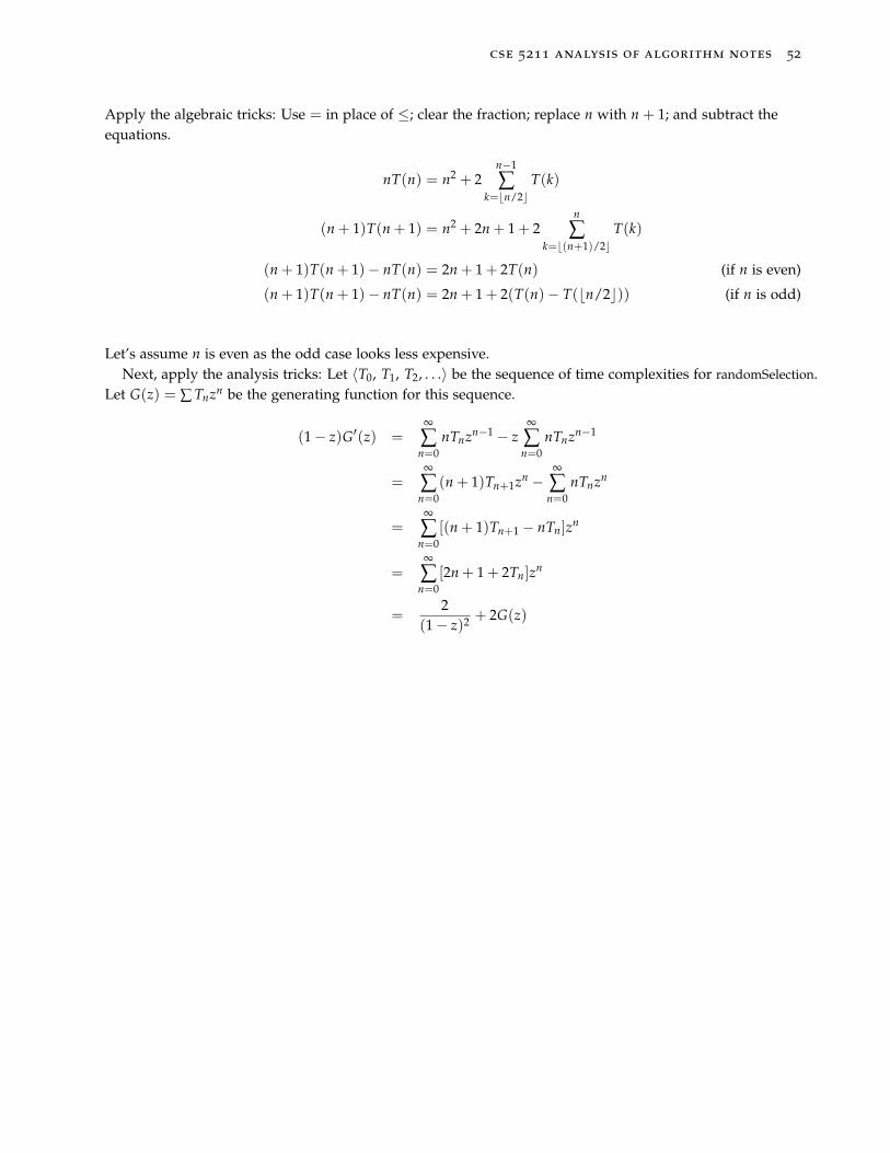
cse 5211 analysis of algorithm notes 52
Apply the algebraic tricks: Use = in place of ≤; clear the fraction; replace n with n + 1; and subtract theequations.
nT(n) = n2 + 2n−1
∑k=bn/2c
T(k)
(n + 1)T(n + 1) = n2 + 2n + 1 + 2n
∑k=b(n+1)/2c
T(k)
(n + 1)T(n + 1)− nT(n) = 2n + 1 + 2T(n) (if n is even)
(n + 1)T(n + 1)− nT(n) = 2n + 1 + 2(T(n)− T(bn/2c)) (if n is odd)
Let’s assume n is even as the odd case looks less expensive.Next, apply the analysis tricks: Let 〈T0, T1, T2, . . .〉 be the sequence of time complexities for randomSelection.
Let G(z) = ∑ Tnzn be the generating function for this sequence.
(1− z)G′(z) =∞
∑n=0
nTnzn−1 − z∞
∑n=0
nTnzn−1
=∞
∑n=0
(n + 1)Tn+1zn −∞
∑n=0
nTnzn
=∞
∑n=0
[(n + 1)Tn+1 − nTn]zn
=∞
∑n=0
[2n + 1 + 2Tn]zn
=2
(1− z)2 + 2G(z)
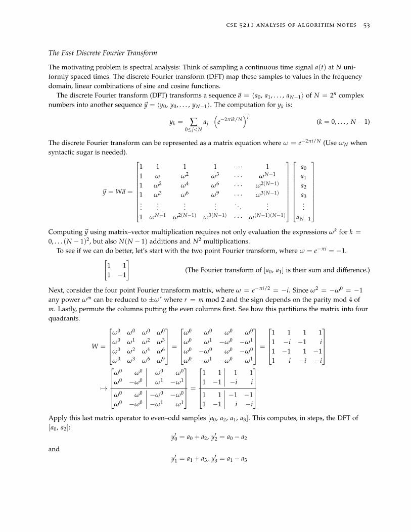
cse 5211 analysis of algorithm notes 53
The Fast Discrete Fourier Transform
The motivating problem is spectral analysis: Think of sampling a continuous time signal a(t) at N uni-formly spaced times. The discrete Fourier transform (DFT) map these samples to values in the frequencydomain, linear combinations of sine and cosine functions.
The discrete Fourier transform (DFT) transforms a sequence~a = 〈a0, a1, . . . , aN−1〉 of N = 2n complexnumbers into another sequence ~y = 〈y0, y0, . . . , yN−1〉. The computation for yk is:
yk = ∑0≤j<N
aj ·(
e−2πik/N)j
(k = 0, . . . , N − 1)
The discrete Fourier transform can be represented as a matrix equation where ω = e−2πi/N (Use ωN whensyntactic sugar is needed).
~y = W~a =
1 1 1 1 · · · 11 ω ω2 ω3 · · · ωN−1
1 ω2 ω4 ω6 · · · ω2(N−1)
1 ω3 ω6 ω9 · · · ω3(N−1)
......
......
. . ....
1 ωN−1 ω2(N−1) ω3(N−1) · · · ω(N−1)(N−1)
a0
a1
a2
a3...
aN−1
Computing ~y using matrix–vector multiplication requires not only evaluation the expressions ωk for k =
0, . . . (N − 1)2, but also N(N − 1) additions and N2 multiplications.To see if we can do better, let’s start with the two point Fourier transform, where ω = e−πi = −1.[
1 11 −1
](The Fourier transform of [a0, a1] is their sum and difference.)
Next, consider the four point Fourier transform matrix, where ω = e−πi/2 = −i. Since ω2 = −ω0 = −1any power ωm can be reduced to ±ωr where r = m mod 2 and the sign depends on the parity mod 4 ofm. Lastly, permute the columns putting the even columns first. See how this partitions the matrix into fourquadrants.
W =
ω0 ω0 ω0 ω0
ω0 ω1 ω2 ω3
ω0 ω2 ω4 ω6
ω0 ω3 ω6 ω9
=
ω0 ω0 ω0 ω0
ω0 ω1 −ω0 −ω1
ω0 −ω0 ω0 −ω0
ω0 −ω1 −ω0 ω1
=
1 1 1 11 −i −1 i1 −1 1 −11 i −i −i
7→
ω0 ω0 ω0 ω0
ω0 −ω0 ω1 −ω1
ω0 ω0 −ω0 −ω0
ω0 −ω0 −ω1 ω1
=
1 1 1 11 −1 −i i
1 1 −1 −11 −1 i −i
Apply this last matrix operator to even–odd samples [a0, a2, a1, a3]. This computes, in steps, the DFT of[a0, a2]:
y′0 = a0 + a2, y′2 = a0 − a2
andy′1 = a1 + a3, y′3 = a1 − a3
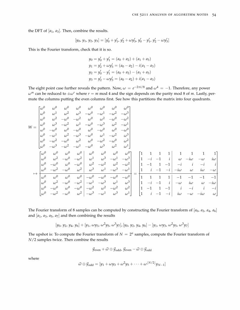
cse 5211 analysis of algorithm notes 54
the DFT of [a1, a3]. Then, combine the results.
[y0, y1, y2, y3] = [y′0 + y′1, y′2 + ωy′3, y′0 − y′1, y′2 −ωy′3]
This is the Fourier transform, check that it is so.
y0 = y′0 + y′1 = (a0 + a2) + (a1 + a3)
y1 = y′2 + ωy′3 = (a0 − a2)− i(a1 − a3)
y2 = y′0 − y′1 = (a0 + a2)− (a1 + a3)
y3 = y′2 −ωy′3 = (a0 − a2) + i(a1 − a3)
The eight point case further reveals the pattern. Now, ω = e−2πi/8 and ω4 = −1. Therefore, any powerωm can be reduced to ±ωr where r = m mod 4 and the sign depends on the parity mod 8 of m. Lastly, per-mute the columns putting the even columns first. See how this partitions the matrix into four quadrants.
W =
ω0 ω0 ω0 ω0 ω0 ω0 ω0 ω0
ω0 ω1 ω2 ω3 −ω0 −ω1 −ω2 −ω3
ω0 ω2 −ω0 −ω2 ω0 ω2 −ω0 −ω2
ω0 ω3 −ω2 ω1 −ω0 −ω3 ω2 −ω1
ω0 −ω0 ω0 −ω0 ω0 −ω0 ω0 −ω0
ω0 −ω1 ω2 −ω3 −ω0 ω1 −ω2 ω3
ω0 −ω2 −ω0 ω2 ω0 −ω2 −ω0 ω2
ω0 −ω3 −ω2 −ω1 −ω0 ω3 ω2 ω1
7→
ω0 ω0 ω0 ω0 ω0 ω0 ω0 ω0
ω0 ω2 −ω0 −ω2 ω1 ω3 −ω1 −ω3
ω0 −ω0 ω0 −ω0 ω2 −ω2 ω2 −ω2
ω0 −ω2 −ω0 ω2 ω3 ω1 −ω3 −ω1
ω0 ω0 ω0 ω0 −ω0 −ω0 −ω0 −ω0
ω0 ω2 −ω0 −ω2 −ω1 −ω3 ω1 ω3
ω0 −ω0 ω0 −ω0 −ω2 ω2 −ω2 ω2
ω0 −ω2 −ω0 ω2 −ω3 −ω1 ω3 ω1
=
1 1 1 1 1 1 1 11 −i −1 i ω −iω −ω iω1 −1 1 −1 −i i −i i1 i −1 −i −iω ω iω −ω
1 1 1 1 −1 −1 −1 −11 −i −1 i −ω iω ω −iω1 −1 1 −1 i −i i −i1 i −1 −i iω −ω −iω ω
The Fourier transform of 8 samples can be computed by constructing the Fourier transform of [a0, a2, a4, a6]
and [a1, a3, a5, a7] and then combining the results
[y0, y2, y4, y6] + [y1, ωy3, ω2y5, ω3y7], [y0, y2, y4, y6]− [y1, ωy3, ω2y5, ω3y7]
The upshot is: To compute the Fourier transform of N = 2n samples, compute the Fourier transform ofN/2 samples twice. Then combine the results
~yeven + ~ω⊕~yodd, ~yeven − ~ω⊕~yodd
where~ω⊕~yodd = [y1 + ωy3 + ω2y5 + · · ·+ ωbN/2cyN−1]
cse 5211 analysis of algorithm notes 55
Cooley and Tukey (Cooley and Tukey, 1965) are credited with discovering how to make the discrete Fouriertransform fast by exploiting facts about polynomials and roots of unity. Their fast discrete Fourier transform(FDFT) computes the values yk, k = 0, . . . , N − 1 in O(N lg N) steps. A huge improvement.
To better understand the FDFT some basic facts are needed. Consider the problem in terms of polyno-mials. Let
y(x) = a0 + a1x + a2x2 + a3x3 + · · ·+ aN−1xN−1
be a polynomial of degree N − 1. The polynomial can be split by the parity (even or odd) of its coefficients.
yeven(x) = a0 + a2x + a4x2 + · · ·+ aN−2xN/2−1
andyodd(x) = a1 + a3x + a5x2 + · · ·+ aN−1xN/2−1
and y(x) can be reconstructed byy(x) = yeven(x2) + xyodd(x2) (18)
The DFT calls for evaluating y(x) at x = ωk = e−2πik/N for k = 0, . . . , N − 1. This reduces to evaluatingyeven(x2) and yodd(x2) at x2 = ωk = e−4πik/N for 0 ≤ k < N/2.
The values ωk are N-th complex roots of unity: They lie on the unit circle in the complex plain.(ωk)N
= e−2πik = cos 2πk− i sin 2πk = 1 (0 ≤ k < N − 1)
The principal N-th root of unity isω = ωN = e−2πi/N
Further,
ωN/2 =(
e−2πi/N)N/2
= e−πi = −1
ωk+N/2 =(
e−2πi(k+N/b2)= e−2πike−πiN = −ωk(
ωk+N/2)2
=(
e−2πi(2k+N)= e−2πi(2k) = (ωk)2
Developing the Cooley–Tukey FFT in Haskell
Here’s Haskell code 3 for the fast discrete Fourier transform. The 3 I am indebted to a former student,Cristhian Cruz Espinoza, for theHaskell code structure.
outline for the fft module is simple: Import other needed modules,define other functions as needed, and include a main function for IOand testing.
55a 〈FFT 55a〉≡module FFT ( fft ) where
〈Import external modules 55b〉〈Auxiliary functions 56a〉〈Main function 57〉The Complex data type is needed for constructing complex numbers and performing arithmetic on val-
ues of this type.
55b 〈Import external modules 55b〉≡import Data.Complex
cse 5211 analysis of algorithm notes 56
Looking forward, here are descriptions of the functions that will be needed. The value n is what hasbeen called N previously, a quirk of Haskell here.
56a 〈Auxiliary functions 56a〉≡〈Compute a root of unity e(−2πk/n)j
56b〉〈Split the list into even and odd lists 56c〉〈Combine the lists 56d〉〈Cooley-Tukey FDFT 56e〉The mkPolar function maps an amplitude r and phase θ to complex number reθi = r(cos θ + i sin θ). For
roots of unity, the amplitude is r = 1, and the phase is θ = −2πijk/n.
56b 〈Compute a root of unity e(−2πk/n)j56b〉≡
cmpExp n k j = mkPolar 1 (-2 * pi * fromIntegral k / fromIntegral n) * j
To apply the recursion, the list of samples must be split into two pairs: The first list contains samplewith even indexes; the second contains odd indexed samples.
56c 〈Split the list into even and odd lists 56c〉≡splitEvenOdd [] = ([], [])
splitEvenOdd [x] = ([x],[])
splitEvenOdd (x:y:xs) = (x:xe, y:yo)
where (xe, yo) = splitEvenOdd xs
Combine the two lists into one. The recursion requires concatenating the sum and difference of the twolists:
56d 〈Combine the lists 56d〉≡combine [] [] = []
combine xs [] = xs
combine [] ys = ys
combine xs ys = add ++ sub
where add = zipWith (+) xs ys
sub = zipWith (-) xs ys
56e 〈Cooley-Tukey FDFT 56e〉≡fft :: [Complex Double] -> [Complex Double]
fft [] = []
fft [x] = [x]
fft xs = combine even cmpOdd
where (e, o) = splitEvenOdd xs
even = fft e
odd = fft o
size = length xs
cmpOdd = zipWith (cmpExp size) [0..] odd
Testing the code
Okay, we’ve got some code, let’s test that it works as expected. Interactive tests are good for unit testingfunctions.
cse 5211 analysis of algorithm notes 57
Unit Tests with ghci
The Haskell source (should be) here. The small sample script below will get you started. The script showsthe results of tests on computing roots of unity, splitting and combining lists, and the computing theFourier transform.
Recall the values cmpExp n k j= (ωk)j = e−2πkj/n are used in evalu- Verify the results in thescripts and test other com-putations yourself.
Verify the results in thescripts and test other com-putations yourself.
ating values yk in the Fourier transform.
yk = ∑0≤j<n
ajωkj
Therefore, cmpExp 2 0 1= e−2π0·1/2 = 1 is computed correctly, but there is round-off error in the imagi-nary part of cmpExp 2 1 1.
% ghci
GHCi, version (your version \#): http://www.haskell.org/ghc/ :? for help
Prelude> :l FFT.hs
[1 of 1] Compiling Main ( FFT.hs, interpreted )
Ok, modules loaded: Main.
*FFT> cmpExp 2 0 1
1.0 :+ 0.0
*FFT> cmpExp 2 1 1
(-1.0) :+ (-1.2246467991473532e-16)
*FFT> splitEvenOdd [0,1,2,3]
([0,2],[1,3])
combine [1,2] [3,4]
[4,6,-2,-2]
*FFT> fft [1,1]
[2.0 :+ 0.0,0.0 :+ 0.0]
Integration Tests with ghc
The topic of the class is analysis of algorithms. Theory says the time Analyze the time com-plexities of splitEvenOdd,combine, and fft.
Analyze the time com-plexities of splitEvenOdd,combine, and fft.
complexity is modeled by some function in Θ(N lg N) = Θ(2nn)where N = 2n is the number of samples. Does running the fft codeproduce running times that fit this model?
The noweb source file FFT.nw is here. Running notangle FFT.nw >
FFT.hs generates the Haskell source FFT.hs Runningnoweave -index
-delay FFT.nw > FFT.tex generates the LATEX source FFT.tex The Compile the code with profil-ing options, collect run timedata and compare your ex-periment with theory.
Compile the code with profil-ing options, collect run timedata and compare your ex-periment with theory.
overall idea of the main function is simple: Read an integer n; createa list of N = 2n (random) complex numbers; compute their Fouriertransform; and show the results.
57 〈Main function 57〉≡main :: IO()
main = interact (show . fft . createList . read)

cse 5211 analysis of algorithm notes 58
A list of N = 2n random complex numbers will be generated. To do this, the System.Random modulewill be used.
58a 〈Import external modules 55b〉+≡import System.Random
To generate a list of complex numbers, create lists of real and imaginary parts, and zip them togetherwith the Complex number constructor :+.
58b 〈Auxiliary functions 56a〉+≡〈Create a list of random complex numbers 58c〉
58c 〈Create a list of random complex numbers 58c〉≡createList :: Int -> [Complex Double]
createList n = take (2^n) $ zipWith (:+) (randoms (mkStdGen 10)) (randoms (mkStdGen 10))
References
Cooley, J. W. and Tukey, J. W. (1965). An algorithm for the machine calculation of complex Fourier series.Mathematics of Computation, 19(90):297–301. [page 55]

cse 5211 analysis of algorithm notes 59
Numerical Analysis
An approximate answer to the right problem is worth a good deal more than an exactanswer to an approximate problem.
John Tukey
Much of early computing revolved around numerical algorithms that produce values that approximatethe True value. Approximation algorithms can be terminated once a computed value is determined to begood enough. To illustrate numerical algorithms, let’s develop Newton’s method for computing an x suchthat f (x) = 0. In particular, we’ll illustrate the method to approximate
√m.
Newton’s Method
A classic numeric problem is: Given a function f : R 7→ R, compute roots (zeros) x such that f (x) = 0.In Western society, Newton’s name is attached to one method for computing roots. But the roots of themethod can be traced to ancient mathematicians of Mesopotomia, the region of modern day Iraq and Iran.Clay tablets from Mesopotamia, dated between 1800 B.C. to 1600 B.C., showing how to approximate
√2
and perform other arithmetic operations have been found. Algorithms that compute numbers like√
2 or π
do not terminate: There is no finite positional notation for these numbers.Newton is credited with generalizing the nascent idea to a broad class of functions. An example func-
tion is f (m) = x2 − m, which has root x =√
m. The idea is: Let x be a zero of function f . Use Taylor’stheorem. Solve for x, and discard the second order error.
0 = f (x) ≈ f (xk) + f ′(xk)(x− xk) +f ′′(ξ)
2(x− xk)
2
x = xk −f (xk)
f ′(xk)− f ′′(ξ)
2 f ′(xk)(x− xk)
2
x ≈ xk −f (xk)
f ′(xk)
For the function f (x) = x2 − 2 the approximation reduces to
x ≈ xk −x2
k − 22xk
=xk + 2/xk
2
The approximation is the average of xk > 0 and 2/xk. If xk is too small: x2k − 2 < 0, then 2/xk is too large:
((0 < 2− x2k)⇒ (0 < 2/x2
k − 1))⇒ ((2/xk)2 − 2 > 0)
The average of xk and 2/xk is a better approximation.
• Start with h0 = 1 as an initial approximation to√
2
• Clearly 1 is too small, as the Babylonians could easily measure
• But, if 1 =√
2, then 1 · 1 =√
2 ·√
2 = 2 and so 2/1 =√
2
• As it is, 2/1 is too large
• The average of the under estimate 1 and the over estimate 2/1 provides a better approximation to√
2,call this
h1 =12
(h0 +
2h0
)=
12
(1 +
21
)=
32
cse 5211 analysis of algorithm notes 60
• But h1 = 3/2 is too large, as the Babylonians could measure
• But, if 3/2 were the exact square root, then 2/(3/2) = 4/3 would equal√
2
• As it is, 4/3 ≈ 1.333 · · · is too small
• The average of the over estimate 3/2 and the under estimate 4/3 will provide a better approximation
h2 =12
(h1 +
2h1
)=
12
(32+
43
)=
1712≈ 1.41166 · · ·
• But h2 = 17/12 is too small
• The Babylonians carried out this iteration more times computing the√
2 accurately to at least 9 decimalplaces
• That is, they next computed the average of h2 = 17/12 and 2/h2 = 24/17
h3 =12
(h2 +
2h2
)=
12
(1712
+2417
)=
12
(289 + 28817× 12
)≈ 1.41421568628 · · ·
To generalize the√
2 method, pretend you want to compute√
m. This is equivalent to computing a solu-tion to the equation
x2 −m = 0
Consider the recurrence equation
xk =xk−1 + m/xk−1
2, k ≥ 1 (19)
Given an initial value x0, equation 19 can be used to generate a sequence
〈x0, x1, x2, . . .〉 .
If you pretend that xk converges to x as k goes to infinity, that is,
limk→∞
xk = x
Then x satisfies the equations
x =x + m/x
22x = x + m/x
x = m/x
x2 = m
x =√
m

cse 5211 analysis of algorithm notes 61
Implementing Newton’s method in Haskell
A first step in implementing Newton’s method for computing√
m is to define the function that maps mand xk−1 to the next value xk.
61a 〈Newton 61a〉≡module Newton ( newton ) where
〈Apply the recursion 61b〉〈Repeatedly apply f to x 61c〉〈Test if successive values meet a relative tolerance 62a〉〈Newton’s square root 62b〉
The recursion is
xk+1 = xk −f (xk)
f ′(xk)where f (x) = x2 − 2
61b 〈Apply the recursion 61b〉≡next :: Double -> Double -> Double
next m 0 = error "Division by zero"
next m x = (x + m/x)/2
We want to repeatedly apply next to some initial value and generate a list of Doubles. Let’s definerepeatedly to be a function that applies a function f :: Double −> Double to itself repeatedly. An initialvalue (seed) a for f starts the iteration, generating an infinite list.
61c 〈Repeatedly apply f to x 61c〉≡repeatedly :: (Double -> Double) -> Double -> [Double]
repeatedly f a = a : repeatedly f (f a)
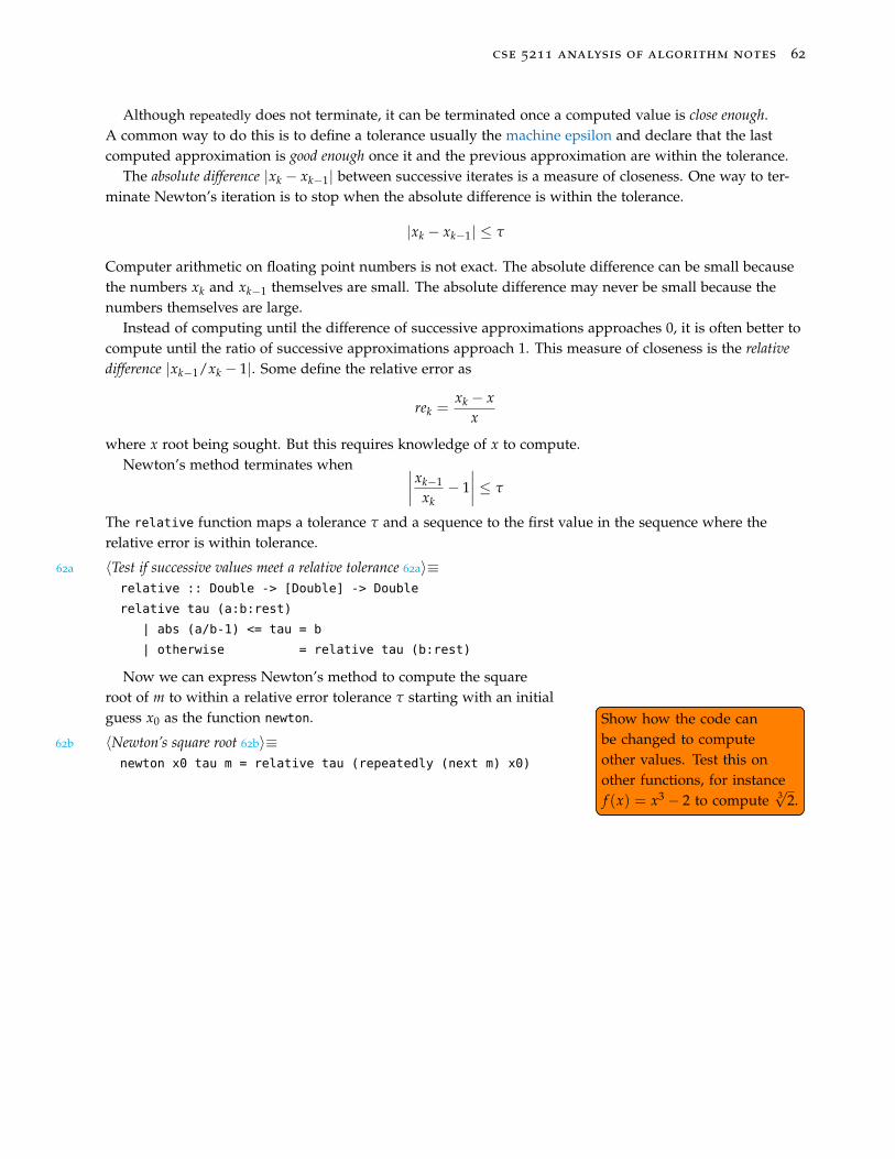
cse 5211 analysis of algorithm notes 62
Although repeatedly does not terminate, it can be terminated once a computed value is close enough.A common way to do this is to define a tolerance usually the machine epsilon and declare that the lastcomputed approximation is good enough once it and the previous approximation are within the tolerance.
The absolute difference |xk − xk−1| between successive iterates is a measure of closeness. One way to ter-minate Newton’s iteration is to stop when the absolute difference is within the tolerance.
|xk − xk−1| ≤ τ
Computer arithmetic on floating point numbers is not exact. The absolute difference can be small becausethe numbers xk and xk−1 themselves are small. The absolute difference may never be small because thenumbers themselves are large.
Instead of computing until the difference of successive approximations approaches 0, it is often better tocompute until the ratio of successive approximations approach 1. This measure of closeness is the relativedifference |xk−1/xk − 1|. Some define the relative error as
rek =xk − x
x
where x root being sought. But this requires knowledge of x to compute.Newton’s method terminates when ∣∣∣∣ xk−1
xk− 1∣∣∣∣ ≤ τ
The relative function maps a tolerance τ and a sequence to the first value in the sequence where therelative error is within tolerance.
62a 〈Test if successive values meet a relative tolerance 62a〉≡relative :: Double -> [Double] -> Double
relative tau (a:b:rest)
| abs (a/b-1) <= tau = b
| otherwise = relative tau (b:rest)
Now we can express Newton’s method to compute the squareroot of m to within a relative error tolerance τ starting with an initialguess x0 as the function newton. Show how the code can
be changed to computeother values. Test this onother functions, for instancef (x) = x3 − 2 to compute 3
√2.
Show how the code canbe changed to computeother values. Test this onother functions, for instancef (x) = x3 − 2 to compute 3
√2.
62b 〈Newton’s square root 62b〉≡newton x0 tau m = relative tau (repeatedly (next m) x0)

cse 5211 analysis of algorithm notes 63
Convergence of Newton’s Method
The number of times the (next m) function is evaluated measures the time complexity of the mysqrt al-gorithm. It is not obvious what this number is. What can be shown is that Newton’s method convergesquadratically, under certain assumptions that are often True.
There is a more elegant, more general proof of the quadratic convergence of Newton’s method. But thisis beyond the scope of these notes.
Consider the function f (x) = x2 −m. Using Taylor’s theorem, you can derive the equation
x2 −m = (x2k−1 −m) + 2xk−1(x− xk−1) + (x− xk−1)
2
Pretend that x =√
m so that both sides of the above equation are zero. Divide by 2xk−1 to get
0 = (x2k−1 −m)/2xk−1 + (x− xk−1) + (x− xk−1)
2/2xk−1
Notice that(x2
k−1 −m)/2xk−1 − xk−1 = −(x2k−1 + m)/2xk−1 = −xk
Therefore,
xk − x = (xk−1 − x)2/2xk−1 or
ek =e2
k−12xk−1
That is, the absolute error xk − x at step k is proportional to the square of the error at step k− 1. When theerror is less than 1, the number of correct digits doubles with each iteration.
In the general case, assume that function f has a continuous second derivative. Assume x is a root of f ,that is f (x) = 0. By Taylor’s theorem
0 = f (x) ≈ f (xk) + f ′(xk)(x− xk) +f ′′(ξ)
2(x− xk)
2
x = xk −f (xk)
f ′(xk)− f ′′(ξ)
2 f ′(xk)(x− xk)
2
x ≈ xk −f (xk)
f ′(xk)
cse 5211 analysis of algorithm notes 64
Amortized Cost Models
A loan is amortized when it is paid down in sequence of equal payments with a fixed in-terest rate. The payments are composed of principal and interest. Early on, the interest is high and theprincipal is low. Overtime, the interest amount charged to interest goes down and the principal reduces theamount owed more quickly.
Geometric sums describe amortization. A typical mortgage starts by borrowing an amount P at a fixedannual interest rate r to be paid off in monthly over y years. The monthly interest rate is i = r/12 and thenumber of payments is t = 12y.
The amount owed initially is P0 = P. At the beginning of month t ≥ 1, the amounted owed is theamount owed at month t− 1 plus the interest on that amount, minus the amount paid to reduce the loan.
Pt = Pt−1(1 + i)− A
Rolling up (or down) this recurrence, see that
Pt = P(1 + i)t − At−1
∑j=0
(1 + i)j = P(1 + i)t − A(1 + i)t − 1
i
The value of A, the monthly payments, where P(t) = 0 is sought, and with a little bit of algebra, computethat
A = Pi(1 + i)n
(1 + i)t − 1
loans can become scary when you compare how much you’ll pay At with how much you borrowed P.
Amortized analysis guarantees the average cost performance of each operation in a
sequence in the worst case. Imagine a data structure where each time some operation is performed,its structure changes so that the next operation should be quicker. There are at least three ways to computeamortized costs: (1) Aggregate analysis, (2) the accounting method, and (3) the potential method.
Queues in Haskell
Pretend you need to implement a first-in, first-out queue in afunctional language. 4 The queue data structure minimally defines 4 I’m indebted to Rafal’s Blog for the
structure of the codeenqueue to place a value last , and dequeue to remove the head. Anaive implementation uses a list to implement a queue.
Queue data structure1 enqueue : : a −> [ a ] −> [ a ]2 enqueue e q = ( q ++ [ e ] )3
4 dequeue : : [ a ] −> ( a , [ a ] )5 dequeue [ ] = ( undefined , [ ] )6 dequeue q = ( head q , t a i l q )
Exercise: Why is this list-based implementation of enqueue too expensive?
cse 5211 analysis of algorithm notes 65
Using two stacks to implement a queue
Using two stacks and amortized analysis, Queue can be implemented efficiently. The idea is pushing valueson a first stack, then popping and pushing them onto a second stack presents the values in first-in, first-outorder.
To support this, define a new datatype Queue that contains two stacks (lists): An inbox and an outbox.
1 data Queue a = Queue 2 inbox : : [ a ] ,3 outbox : : [ a ]4 deriving ( Eq , Show)
To enqueue a value, push it to inbox.
1 enqueue : : a −> Queue a −> Queue a2 enqueue e ( Queue inbox outbox ) = Queue ( e : inbox ) outbox
The time complexity of enqueue is O(1).Dequeuing a value returns an ordered pair: The value at the head of the queue and the new queue.There are two cases consider when dequeuing a value.
1. If outbox is empty, pop from inbox to outbox until inbox is empty. This can be done by setting the reverseof inbox to the outbox, and setting the inbox to empty. Return value returned is then the head of theoutbox with its tail.
2. If outbox is not empty, return its head and the Queue containing the inbox and the tail of outbox.
1 data Queue a = Queue 2 inbox : : [ a ] ,3 outbox : : [ a ]4 deriving ( Eq , Show)5
6 enqueue : : a −> Queue a −> Queue a7 enqueue e ( Queue inbox outbox ) = Queue ( e : inbox ) outbox8
9 dequeue : : Queue a −> ( a , Queue a )10 dequeue ( Queue inbox [ ] ) = dequeue $ Queue [ ] ( reverse inbox )11 dequeue ( Queue inbox outbox ) = ( head outbox , Queue inbox ( t a i l outbox ) )
In the first case, the time complexity of dequeue depends on the the time complexity of reverse, which isO(n). The Haskell prelude definition of reverse is
1 reverse : : [ a ] −> [ a ]2 reverse = f o l d l ( f l i p ( : ) ) [ ]
which starting from the empty list builds the reverse from the left using the cons operation : flipping thevalue with the list. In the second case, the time complexity of dequeue depends the cost of taking a head,O(1) and a tail O(1).
Amortized cost of Haskell queue
Consider a sequence of n enqueue, m dequeue operations. It makes sense have the condition m ≤ n.

cse 5211 analysis of algorithm notes 66
In a sequence of operations, each value is pushed onto inbox only once, moved to the outbox at mostonce. and removed from outbox at most once. Each of these are O(1) operations. Thus, averaged over se-quence of operations has amortized cost O(1), even though dequeue can be expensive sometimes.
The aggregate method computes the amortized cost by determining an upper bound T(k) on the totalcost of a sequence of k operations. In the worst case sequence of operations, is n enqueues, followed by 1dequeue. Here, T(k) = n + n where k = n + 1 and the amortized cost is
Tamortized (
2 nn + 1 = O(2)
The accounting method computes the amortized cost by assigning a actual cost and a credit to opera-tions. For instance, enqueue can be charged a cost of 2, its actual cost plus a credit of 1 for when the valuewill be dequeued. A sequence of n enqueues builds a credit of n which is consumed when followed by adequeue.
The potential method computes the amortized cost by determining an
Hash Tables
Consider the problem of hashing values to a table. Typically, in imperative languages, the table is imple-mented as an array ~A with a length allocated when it was created. When too many values are hashed to~A, collisions occur. A common solution is to create a new larger array ~A′, copy the values in ~A into it, andclean up the memory used by ~A. This is an expensive operation, especially when compared to the oftenused insert operation, which has O(1) cost.
Consider a sequence of insert operations, where the table starts of length 1 and doubles each time anoverflow occurs. It is convenient to measure the cost of doubling the table by the expression 1 + 2k fork = 0, 1, . . .. The table summarizes the cost analysis.
Item 1 2 3 4 5 6 7 8 9 10 · · ·Table size 1 2 4 4 8 8 8 8 16 16 · · ·Cost 1 2 3 1 5 1 1 1 9 1 · · ·
The amortized cost per operation is O(1) for a sequence of n insertions into a table.
Amortized cost =1 + 2 + 3 + 1 + 5 + 1 + 1 + 1 + 9 + · · ·
n
=1 + (1 + 1) + (1 + 2) + 1 + (1 + 4) + 1 + 1 + 1 + (1 + 8) + · · ·
n
=
n terms︷ ︸︸ ︷(1 + 1 + 1 + 1 + 1 + · · · )
n+
blg (n−1)c+1 terms︷ ︸︸ ︷(1 + 2 + 4 + 8 ++ · · · )
n
≤ n + 2nn
= 3
Note
∑0≤k≤lg (n−1)
2k = 2lg (n−1)+1 − 1 = 2(n− 1)− 11
cse 5211 analysis of algorithm notes 67
Greedy Algorithms
Greedy heuristic Make a choice that seems best at the moment. This locally optimal choicemay lead to a globally optimal solution. However, greedy algorithms don’t always work. Deciding how tomake good local choices is key.
Combinatorial Optimization
Greedy algorithms are often used to solve combinatorial optimization problems. Given an instance I of a func-tion problem P , assume there is a set of candidate or feasible solutions that satisfy the constraints of the prob-lem. For each feasible solution there is a value determined by an objective function. Find one (or more)optimal solution(s) that minimize (or maximize) the value the the objective function.
For a greedy algorithm to work, an optimal solution to a problem must have optimal solutions to sub-problems.One way to learn about greedy algorithms is to study examples.
Making Change
Working a cash register is a common example of greedy approaches. Raise your hand if youunderstand the problem and its solution.
Pretend a cashier needs to give a customer $2.73 in change. How can the cashier make the change usingthe fewest coins and/or bills?
The abstraction is this: A value V to be represented in denominations d0, d1, . . . , dn−1 as a sum
V = a0d0 + a1d1 + · · ·+ an−1dn−1
such that the number of “coins”
a0 + a1 + · · ·+ an−1 is as small as possible
The greedy approach is very Euclidean algorithm-like:
1. Preconditions: Assume all the a’s are set to 0, and the denominations are sorted in decreasing order.
2. Find the largest denomination dk ≤ V.
3. Divide dk into V
• If the remainder R = 0 stop with the quotient set to ak.
• Otherwise, start again from step 2 with V replaced by the remainder R.
Ignoring the preconditions, the algorithm takes at most n steps, the number of denominations.Greedy coin changing computes the optimal (minimal number of coins) for some collections of denom-
inations, but not for all. It is optimal for 1, 5, 10, 25, 50, 100, where the proof is by cases and induction onV. It is not optimal for 1, 10, 21, 34, 70, 100. Consider 140.
cse 5211 analysis of algorithm notes 68
Tape Storage of Files
Okay, it is old-school, but the problem: How to store files on tape helps illustrate greedy algorithms. Pre-tend there are n files to be stored on a tape. Let L[i] be the length of file i for i = 1, 2, . . . , n. Assume thecost of accessing a file depends on its length plus the lengths of prior files on the tape, call this sequentialaccess time. The time to access file k is
T(k) =k
∑i=1
L[i]
If each file is equally likely to be accessed, then the average (expected) time cost is to access a file is
Tavg(n) =1n
n
∑k=1
T(k) =1n
n
∑k=1
k
∑i=1
L[i]
Different file storage orders result in different expected costs. For instance, suppose the files have lengths
L[1] = 100, L[2] = 150, L[3] = 50, L[4] = 200
If the files are stored in order 〈3, 1, 2, 4〉 then the average assess time is
Tavg(n) =14(50 + (50 + 100) + (50 + 100 + 150) + (50 + 100 + 150 + 200))
=14(4 · 50 + 3 · 100 + 2 · 150 + 200) = 250
You can compute that other order increase the average access time. For example, the order 〈1, 2, 3, 4〉 hasaverage cost
Tavg(n) =14(100 + (100 + 150) + (100 + 150 + 50) + (100 + 150 + 50 + 200))
=14(4 · 100 + 3 · 150 + 2 · 50 + 200) = 287.5
Tape Storage Problem: Find permutation π(i) of i = 1, . . . , n that minimizes the average cost.
Tmin-avg(n) = minπ
n
∑k=1
k
∑i=1
L[π(i)]n
There are n! permutations of n distinct values. Therefore, it is infeasible to find the minimum by comput-ing the cost of every permutation, except perhaps for small values of n.
The greedy approach sorts the files by their lengths and stores the shortest length files first. That is,
L[π(i)] ≤ L[π(i + 1)] for all i
And, this greedy approach does produce the smallest average file access cost.Theorem 1. File Access Minimization The average cost of file access is minimized when the files are stored fromsmallest to largest.
Proof. File Access Minimization Suppose that π is the optimal file storage permutation, but two consecu-tive files are out of order by length. Call them file k = π(i) and file j = π(i + 1), k < j. The assumption isthat L[k] > L[j].
If files k and j are swapped, then the cost to access file k is increased by L[j]. And, the cost to access file jis decreased by L[k]. Therefore, the average cost is changed by a negative amount: (L[j]− L[k])/n < 0. But,this contradict that the given order π was one giving minimal average cost for file access.

cse 5211 analysis of algorithm notes 69
Questions and Problems
1. Another greedy approach for tape storage is to store the longest file first. Compare this with the short-est file first heuristic.

cse 5211 analysis of algorithm notes 70
Rational Knapsack Packing
Shortest first is a greedy approach: What can measure shortest? The rational knapsack problemoffers several variant of shortest. The scenario is a set of provisions to place in a knapsack without over-flowing its capacity C. Each resource has a weight and value. The objective is to fill the knapsack achievingmaximum value. And, for the rational problem, fractions of provisions can be used.
Here’s an example: Pretend the knapsack has capacity C = 10 and there are three items with theseweights and values.
w0 = 10, v0 = 30; w1 = 5, v1 = 20; w2 = 1, v2 = 2
And here are some ways to measure shortest:
1. Place lightest first. Place all of item 2, all of 1, and 4/10 of item 0.
Constraint: 1 + 5 +410
10 ≤ 10 Objective: 2 + 20 +4
1030 = 34
2. Place heaviest first. Place all of item 0 and no other items
Constraint: 10 ≤ 10 Objective: 30
3. Place most valuable first. For this instance this approach is the same as heaviest first.
4. Greedy value:weight approach: The sorted value-to-weight ratios arev1
w1= 4;
v0
w0= 3;
v2
w2= 2
Place all of item 1 and 5/10 of item 0.
Constraint: 5 +510
10 ≤ 10 Objective: 20 +5
1030 = 35
The optimal value is 20 + 15 = 35, given by the greedy value-to-weight ratio approach.
Greedy algorithm for Rational Knapsack Packing
The algorithm below uses this greedy heuristic to solve the rational knapsack problem. Its running timeis O(n) if the ratios have be previously computed and sorted. If the ratios need to be sorted its time com-plexity is O(n lg n). Building a heap and using a priority queue may, in some cases, be less expensive thansorting all the ratios. The precondition is
v0
w0≥ v1
w1≥ · · · ≥ vn−1
wn−1
70 〈Rational Knapsack 70〉≡int knapsack(int *v, int *w, int n, int C)
〈Initialize rational knapsack local state 71a〉〈While accumulated weight ≤ C and more items 71b〉
〈If all of the next item can be added 71c〉 〈Update local state 71d〉
〈Otherwise add a fraction of the next item 71e〉
cse 5211 analysis of algorithm notes 71
The local state includes an index k into the value, weight, and fraction arrays. The index k identifies thenext item to be considered. Accumulators for the value and weight are needed, and the fractions can beinitialized to zero.
71a 〈Initialize rational knapsack local state 71a〉≡int k = 0, V = 0, W = 0;
int r[n];
for (int j = 0; j < n; j++) r[j] = 0;
The while condition is this:
71b 〈While accumulated weight ≤ C and more items 71b〉≡while ((W < C) && (k < n))
Inside of the while, test if all of the next item (k)can be placed in the knapsack. This occurs if the currentweight W and the next item’s weight w[k] do not exceed the capacity C.
71c 〈If all of the next item can be added 71c〉≡if (W + w[k] <= C)
When all of the next item fits, update every state value.
71d 〈Update local state 71d〉≡r[k] = 1; W = W + w[k]; V = V + v[k]; k = k + 1;
If not all of the next item fits, the fraction
rk =C−W
wk
determines how much of item k can be placed in the knapsack. Notice that
W + rkwk = C
71e 〈Otherwise add a fraction of the next item 71e〉≡else
r[k] = (C-W)/w[k]; W = C; V = V + r[k]*v[k]; k = k + 1;
Questions and Problems
1. What is the time complexity of the greed value-to-weight rational knapsack algorithm?
cse 5211 analysis of algorithm notes 72
Multiprocessor Scheduling
The multiprocessor scheduling problem (MPS) can be described by the ideas below.
A problem instance: A set T of n tasks, where each task t ∈ T has a positive integer length l(t), and apositive integer m of available processors p.
A feasible solution: A schedule s for all tasks such that each processor executes only one task at a time andeach tasks is scheduled on only one processor.
The objective function: The finishing time f (s) of the last task in the schedule.
An optimal solution: The feasible solutions that minimizes f (s).This function problem can be reduced to a sequence of decision problems: Does schedule s have finish-
ing time less than or equal to a deadline d. Is f (s) ≤ d? This decision problem is NP-complete. Vaguely,this means:
• If a schedule s exists that finishes before or by the deadline d, a non-deterministic algorithm for it is:
– Guess a such a schedule s that meets the deadline
– Test that the finishing time f (s) ≤ d. This can be accomplished in polynomial time.
• The complementary problem seems harder: If no schedule exists every possible schedule must bechecked to prove the deadline is missed.
– A schedule can be imagined as a function from Zn to Zm.
– The number of schedules is then the number of such functions: What is an expression for this count?
– Since there are an exponential number of schedules for two or more processors, the complementaryproblem is hard.
Later, let’s make this more formal by reducing a known NP-complete problem (Partition) to MSP. Thus, ifMSP could be solve in polynomial time, then Partition could be solve in deterministic polynomial time,which does not appear likely.
Greedy algorithm for Multiprocessor Scheduling
A greedy approach often gives acceptable results: Schedule tasks feasibly by longest processing time. Con-sider the tasks sorted in decreasing order. Assign each task to the next, in time, free processor. For exam-ple, with 3 processors and 7 jobs whose lengths are
6, 6, 5, 5, 3, 3, 3
Scanning the list, assign the first three tasks to processors p0, p1, and p2 in that order. For the next task,with length 5, assign it to processor 3, since it is the next, in time, free processor. Then the last three jobsare assigned to processor p0, p1, and p0. Draw a processor-time task scheduled diagram showing this.Thus, the finishing time is 12.
However, an optimal schedule is: Processor 0 executes tasks 0 and 2; processor 1 executes tasks 1 and 3;and, processor 2 executes tasks 4, 5, and 6. with a finishing time of 11.
Here’s some pseudo-code that describes this greedy approach. The array T[] keeps track of when aprocessor will be free.
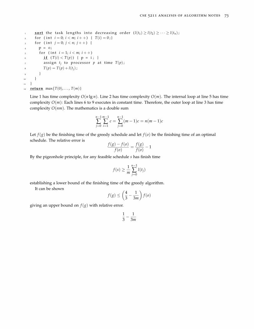
cse 5211 analysis of algorithm notes 73
1 s o r t the task lengths i n t o decreas ing order ( l(t1) ≥ l(t2) ≥ · · · ≥ l(tn) ;2 f o r ( i n t i = 0; i < m; i ++ ) T(i) = 0 ; 3 f o r ( i n t j = 0; j < n; j ++ ) 4 p = 0 ;5 f o r ( i n t i = 1; i < m; i ++ )6 i f ( T(i) < T(p) ) p = i ; 7 ass ign tj to processor p a t time T(p) ;8 T(p) = T(p) + l(tj) ;9
10 11 12 return maxT(0), . . . , T(m)
Line 1 has time complexity O(n lg n). Line 2 has time complexity O(m). The internal loop at line 5 has timecomplexity O(m): Each lines 6 to 9 executes in constant time. Therefore, the outer loop at line 3 has timecomplexity O(nm). The mathematics is a double sum
n−1
∑j=0
m−1
∑i=1
c =n−1
∑j=0
(m− 1)c = n(m− 1)c
Let f (g) be the finishing time of the greedy schedule and let f (o) be the finishing time of an optimalschedule. The relative error is
f (g)− f (o)f (o)
=f (g)f (o)
− 1
By the pigeonhole principle, for any feasible schedule s has finish time
f (s) ≥ 1m
n−1
∑j=0
l(tj)
establishing a lower bound of the finishing time of the greedy algorithm.It can be shown
f (g) ≤(
43− 1
3m
)f (o)
giving an upper bound on f (g) with relative error.
13− 1
3m
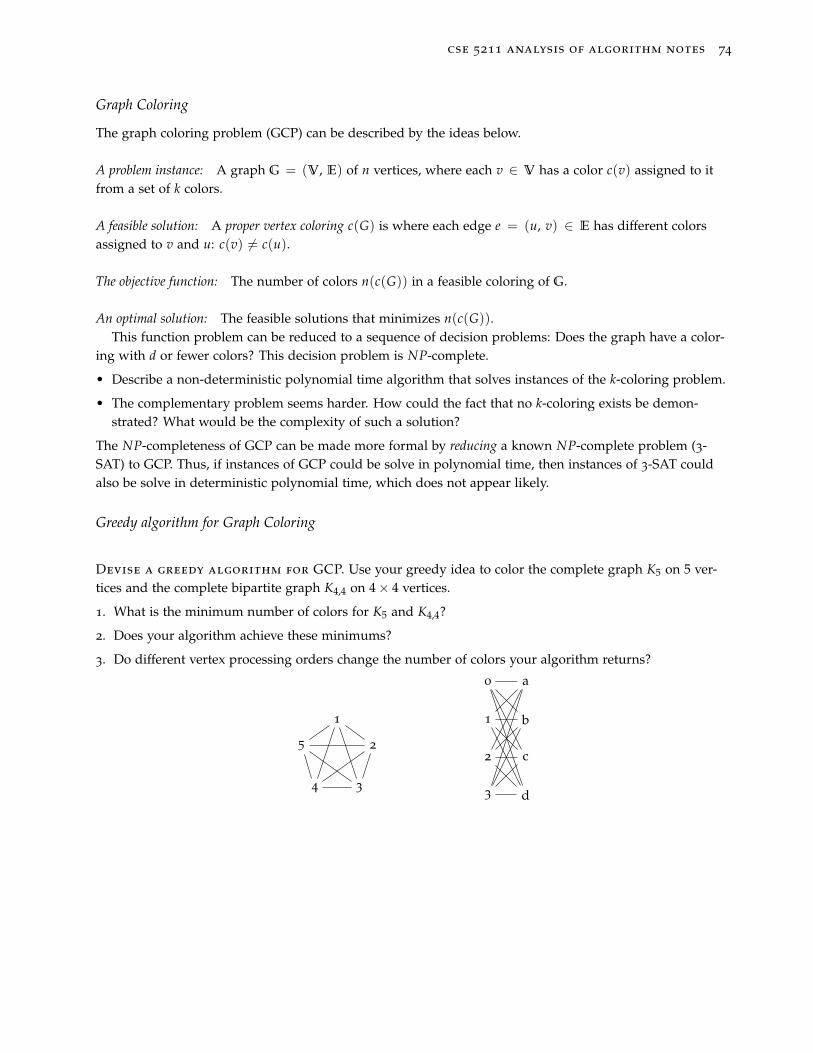
cse 5211 analysis of algorithm notes 74
Graph Coloring
The graph coloring problem (GCP) can be described by the ideas below.
A problem instance: A graph G = (V, E) of n vertices, where each v ∈ V has a color c(v) assigned to itfrom a set of k colors.
A feasible solution: A proper vertex coloring c(G) is where each edge e = (u, v) ∈ E has different colorsassigned to v and u: c(v) 6= c(u).
The objective function: The number of colors n(c(G)) in a feasible coloring of G.
An optimal solution: The feasible solutions that minimizes n(c(G)).This function problem can be reduced to a sequence of decision problems: Does the graph have a color-
ing with d or fewer colors? This decision problem is NP-complete.
• Describe a non-deterministic polynomial time algorithm that solves instances of the k-coloring problem.
• The complementary problem seems harder. How could the fact that no k-coloring exists be demon-strated? What would be the complexity of such a solution?
The NP-completeness of GCP can be made more formal by reducing a known NP-complete problem (3-SAT) to GCP. Thus, if instances of GCP could be solve in polynomial time, then instances of 3-SAT couldalso be solve in deterministic polynomial time, which does not appear likely.
Greedy algorithm for Graph Coloring
Devise a greedy algorithm for GCP. Use your greedy idea to color the complete graph K5 on 5 ver-tices and the complete bipartite graph K4,4 on 4× 4 vertices.
1. What is the minimum number of colors for K5 and K4,4?
2. Does your algorithm achieve these minimums?
3. Do different vertex processing orders change the number of colors your algorithm returns?
1
2
34
5
0
1
2
3
a
b
c
d
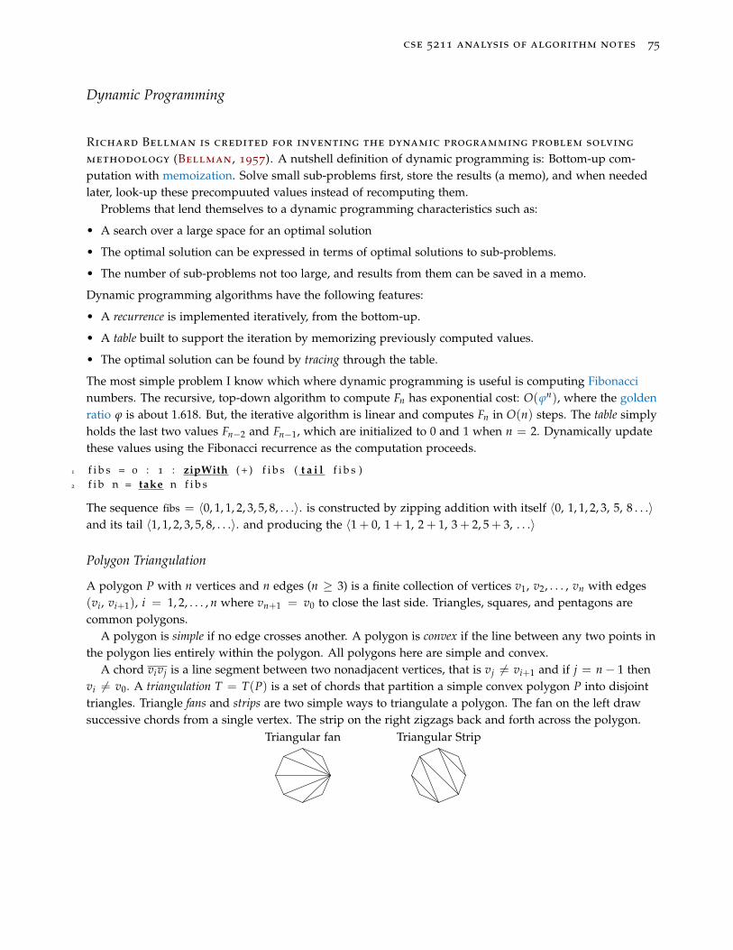
cse 5211 analysis of algorithm notes 75
Dynamic Programming
Richard Bellman is credited for inventing the dynamic programming problem solving
methodology (Bellman, 1957). A nutshell definition of dynamic programming is: Bottom-up com-putation with memoization. Solve small sub-problems first, store the results (a memo), and when neededlater, look-up these precompuuted values instead of recomputing them.
Problems that lend themselves to a dynamic programming characteristics such as:
• A search over a large space for an optimal solution
• The optimal solution can be expressed in terms of optimal solutions to sub-problems.
• The number of sub-problems not too large, and results from them can be saved in a memo.
Dynamic programming algorithms have the following features:
• A recurrence is implemented iteratively, from the bottom-up.
• A table built to support the iteration by memorizing previously computed values.
• The optimal solution can be found by tracing through the table.
The most simple problem I know which where dynamic programming is useful is computing Fibonaccinumbers. The recursive, top-down algorithm to compute Fn has exponential cost: O(ϕn), where the goldenratio ϕ is about 1.618. But, the iterative algorithm is linear and computes Fn in O(n) steps. The table simplyholds the last two values Fn−2 and Fn−1, which are initialized to 0 and 1 when n = 2. Dynamically updatethese values using the Fibonacci recurrence as the computation proceeds.
1 f i b s = 0 : 1 : zipWith ( + ) f i b s ( t a i l f i b s )2 f i b n = take n f i b s
The sequence fibs = 〈0, 1, 1, 2, 3, 5, 8, . . .〉. is constructed by zipping addition with itself 〈0, 1, 1, 2, 3, 5, 8 . . .〉and its tail 〈1, 1, 2, 3, 5, 8, . . .〉. and producing the 〈1 + 0, 1 + 1, 2 + 1, 3 + 2, 5 + 3, . . .〉
Polygon Triangulation
A polygon P with n vertices and n edges (n ≥ 3) is a finite collection of vertices v1, v2, . . . , vn with edges(vi, vi+1), i = 1, 2, . . . , n where vn+1 = v0 to close the last side. Triangles, squares, and pentagons arecommon polygons.
A polygon is simple if no edge crosses another. A polygon is convex if the line between any two points inthe polygon lies entirely within the polygon. All polygons here are simple and convex.
A chord vivj is a line segment between two nonadjacent vertices, that is vj 6= vi+1 and if j = n− 1 thenvi 6= v0. A triangulation T = T(P) is a set of chords that partition a simple convex polygon P into disjointtriangles. Triangle fans and strips are two simple ways to triangulate a polygon. The fan on the left drawsuccessive chords from a single vertex. The strip on the right zigzags back and forth across the polygon.
Triangular fan Triangular Strip

cse 5211 analysis of algorithm notes 76
In practice, some triangulations are better than others. Some optimization goals could be: Minimize thesum of triangle perimeters; minimize the largest area over all the triangles; minimize variation in surfacenormals when the polygon is non-planar.
Minimal Polygon Triangulation
Assume a weight function w(4) = w(vi, vj, vk) is defined on triangles. Let T = T(P) be a triangulation of apolygon P. The objective function is the sum of weights over all triangles.
∑4∈T(P)
w(4)?
Decision Problem: Does triangulation T(P) minimize the sum of weights
∑4∈T
w(4)? (over all triangulations T of P.)
Function Problem: Find optimal triangulations T, those that minimize the sum of weights
∑4∈T
w(4)
Let’s develop a recursion that describes an optimal triangulation.
Polygon Triangulation Recursion
Let’s start by noting some useful facts.
1. Every triangulation of a P is a polygon with n vertices has n sides and n − 3 chords (diameters) thatpartition the polygon into n− 2 triangles. This is an easy induction: Its True for n = 3, a triangle has nochords, and 1 triangle. Appending one new vertex, to a triangulation of an n − 1 vertex polygon addsone chord and one triangle. (Draw pictures)
2. Each polygon edge belongs to one and only one triangle.
3. Each triangle has one or two polygon edges.
4. The number of triangulation grows exponentially. Searching over the entire space is impractical.
Let Cn denote the number of triangulations a simple convex polygon with n + 2 sides (vertices) Drawsome simple cases and convince yourself of the following results.
C1 = 1, C2 = 2, C3 = 5
It is a little harder to enumerate the 6 sided, 6 vertex hexagon, but C(4) = 14. Here’s a drawing fromWikipedia.
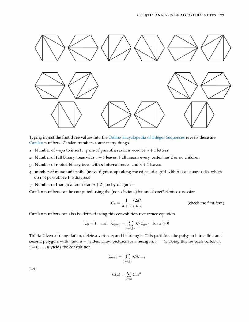
cse 5211 analysis of algorithm notes 77
Typing in just the first three values into the Online Encyclopedia of Integer Sequences reveals these areCatalan numbers. Catalan numbers count many things.
1. Number of ways to insert n pairs of parentheses in a word of n + 1 letters
2. Number of full binary trees with n + 1 leaves. Full means every vertex has 2 or no children.
3. Number of rooted binary trees with n internal nodes and n + 1 leaves
4. number of monotonic paths (move right or up) along the edges of a grid with n× n square cells, whichdo not pass above the diagonal
5. Number of triangulations of an n + 2-gon by diagonals
Catalan numbers can be computed using the (non-obvious) binomial coefficients expression.
Cn =1
n + 1
(2nn
)(check the first few.)
Catalan numbers can also be defined using this convolution recurrence equation
C0 = 1 and Cn+1 = ∑0=i≤n
Ci Cn−i for n ≥ 0
Think: Given a triangulation, delete a vertex vi and its triangle. This partitions the polygon into a first andsecond polygon, with i and n− i sides. Draw pictures for a hexagon, n = 4. Doing this for each vertex vi,i = 0, . . . , n yields the convolution.
Cn+1 = ∑0=i≤n
CiCn−i
LetC(z) = ∑
0≤nCnzn

cse 5211 analysis of algorithm notes 78
be the generating function for the Catalan numbers. Notice the convolution
C(z)C(z) = (C0 + C1z + C2z2 + · · · )(C0 + C1z + C2z2 + · · · )= (C0C0 + [C1C0 + C0C1]z + [C0C2 + C1C1 + C2C0]z2 + · · · )= C1 + C2z + C3z2 + · · ·
ThereforeC(z) = 1 + z[C(z)]2
And by the quadratic formula
C(z) =1−√
1− 4z2z
With some (advanced) calculus and the generalized binomial theorem it can be shown that Cn = 1n+1 (
2nn ).
Computing the Optimal Triangulation
Let W(i, j) be the weight of the optimal triangulation of polygon Pij = (vi, . . . , vj), 1 ≤ i ≤ j ≤ n. That is,
W(i, j) = minT
∑4∈T
w(4)
where T is a triangulation of Pij. We want to know the optimal weight of W(1, n), and the triangulationthat produces it.
In any triangulation Pij = (vi, . . . , vj) of 3 or more vertices there must be one triangle (vi, vk, vj) wherei < k < j. By considering each choice for i < k < j, the problem of computing W(i, j) can be reduced tofinding the minimum of W(i, k) + W(k + 1, j) + w(vi, vk, vj), that is,
W(i, j) =
0 if j− i < 3
min
W(i, k) + W(k + 1, j) + w(vi, vk, vj) : i ≤ k ≤ j
otherwise
To compute the value in row i, column j requires precomputation of values in row i, columns, i to j− 1 andvalues in column j, rows, i + 1 to j.
i i + 1 · · · j · · ·
i W(i, i) W(i, i + 1) · · · W(i, j) · · ·
i + 1...
...... W(i + 1, j) · · ·
......
...... W(i + 2, j) · · ·
j...
...... W(j, j) · · ·
The table of weights of an optimal triangulation can be computed by upward diagonals and the optimalweight W(0, n) found.

cse 5211 analysis of algorithm notes 79
The Memoized Table
Here is a simple example: Let P a five sided pentagon (v1, v2, v3, v4, v5) There are (53) = 10 triangles and
C3 = 5 triangulations, the weights below are made up out of thin air.
4(v1, v2, v3), w(1, 2, 3) = 3
4(v1, v2, v4), w(1, 2, 4) = 6
4(v1, v2, v5), w(1, 2, 5) = 4
4(v1, v3, v4), w(1, 3, 4) = 4
4(v1, v3, v5), w(1, 3, 5) = 7
4(v1, v4, v5), w(1, 4, 5) = 5
4(v2, v3, v4), w(2, 3, 4) = 6
4(v2, v3, v5), w(2, 3, 5) = 3
4(v2, v4, v5), w(2, 4, 5) = 5
4(v3, v4, v5), w(3, 4, 5) = 6
v1
v2
v3 v4
v54 53
v1
v2
v3 v4
v57
63
v1
v2
v3 v4
v54
66
v1
v2
v3 v4
v54
56
v1
v2
v3 v4
v5
6 56
We need to compute values W(i, j) in table below.
j = 1 j = 2 j = 3 j = 4 j = 5
i = 1 W(1, 1) W(1, 2) W(1, 3) W(1, 4) W(1, 5)i = 2 W(2, 2) W(2, 3) W(2, 4) W(2, 5)i = 3 W(3, 3) W(3, 4) W(3, 5)i = 4 W(4, 4) W(4, 5)i = 5 W(5, 5)

cse 5211 analysis of algorithm notes 80
The values on the main and next upper diagonal can be initialized to 0. They represent empty triangles.
j = 1 j = 2 j = 3 j = 4 j = 5
i = 1 0 0 W(1, 3) W(1, 4) W(1, 5)i = 2 0 0 W(2, 4) W(2, 5)i = 3 0 0 W(3, 5)i = 4 0 0i = 5 0
Along the next upper diagonal the values are: The values are the weights of the corresponding triangles:4(1, 2, 3),4(2, 3, 4), 4(3, 4, 5)
j = 1 j = 2 j = 3 j = 4 j = 5
i = 1 0 0 3i = 2 0 0 6i = 3 0 0 6i = 4 0 0i = 5 0
To fill in the next diagonal W(1, 4) is the minimum of 3 + w(1, 3, 4) = (3 + 4) = 7 and 6 + w(1, 2, 4) =
6 + 6 = 12. And, W(2, 5) is the minimum of 6 + w(2, 4, 5) = (6 + 5) = 11 and 6 + w(2, 3, 5) = 6 + 6 = 12
j = 1 j = 2 j = 3 j = 4 j = 5
i = 1 0 0 3 7i = 2 0 0 6 11i = 3 0 0 6i = 4 0 0i = 5 0
Lastly, the value of W(1, 5) is is the minimum of 3 + w(3, 4, 5) = 3 + 6 = 9, 7 + w(1, 4, 5) = (7 + 5) = 12,11 + w(1, 2, 5) = 11 + 4 = 15, and 9 + w(1, 3, 5) = 9 + 7 = 16
j = 1 j = 2 j = 3 j = 4 j = 5
i = 1 0 0 3 7 12i = 2 0 0 6 11i = 3 0 0 6i = 4 0 0i = 5 0
The Trace back
Not only is the optimal weight sought, the triangulation should construct too. This can accomplished byrecording the path to the optimal solution. Let S[i, j] = k if the optimal triangulation of Pij includes thetriangle vi−1, vk, vj
1 publ ic void t r i a n g u l a t e ( Polygon poly ) 2 // i n i t i a l i z e l o c a l s t a t e
cse 5211 analysis of algorithm notes 81
3 i n t n = poly . countOfver t i ces ( ) ;4 double W[ n + 1 ] [ n + 1 ] ;5 double S [ n + 1 ] [ n + 1 ] ;6 f o r ( i n t i = 0 ; i < n ; i ++) W[ i , i ] = 0 ; W[ i , i +1 ]=0 ; 7
8 f o r ( i n t d = 3 ; d <= n ; d++) // f o r every diagonal9 f o r ( i n t i = 1 ; i < n−d ) ; i ++) // f o r every row
10 i n t j = i +d−1; // f i r s t column in a row11 f o r ( i n t k = i +1 ; k <= j ; k++) // f o r every s p l i t t i n g a t k12 w[ i ] [ j ] = ∞ ;13 i n t q = W[ i , k ] + W[ k+1 , j ] + poly . weight ( i , k , j ) ;14 i f ( q < W[ i , j ] ) W[ i , j ] = q ; S [ i , j ] = k ; 15 16 17 18
To compute the time complexity of triangulate
• The initialization in line 6 is O(n).
• Assume the weight function can be computed in constant time. Then the for loop in line 11 is O(j− (i +1) + 1) = O(d− 1).
• Then the loop in line 9 is O(n− (d− 1))(d− 1)
• Finally, recall the sum
∑1≤k<n
(n− k)k =
(n + 1
3
)to simplify the sum
∑1≤d<n
(n− (d− 1))(d− 1) =(
n + 13
)for the loop in line 8.
This algorithm would be useful if its only application was triangulating polygons. The basic idea can beused to solve many problems. See (Sankoff and Kruskal, 1983) for an overview.
References
Bellman, R. (1957). Dynamic Programming. Princeton University Press. [page 75]
Sankoff, D. and Kruskal, J. B., editors (1983). Time Warps, String Edits, and Macromolecules. Addison-Wesley, Reading, Massachusetts. [page 81]
cse 5211 analysis of algorithm notes 82
Dynamic Programming, Part 2
Some dynamic programming algorithms require computing all values in a complete n × mtable. The Edit Distance Problem is an example of this: Find the fewest cost edits to transform string sinto string t, of lengths n and m respectively. The 0–1 Knapsack Problem is too where n is the number ofprovisions and m is the knapsack capacity. Both of these are topics of student reports, so I won’t expandon them here. (The dynamic programming algorithm for the 0–1 Knapsack Problem is not guaranteed tocompute the optimal solution.) Since students are planning to present these problems and algorithms forthem, I will not continue here.
In contrast the polygon triangulation and matrix chain multiplication problems only required fillingan upper triangle of and n × n matrix: (n
2) entries. But, each entry required up to n operations leading toO(n3) algorithms. I’m willing to bet that problems where the number of solutions are Catalan numbershas an O(n3) upper-triangular, dynamic programming algorithm, but I have no proof of this.
Longest Common Subsequence
Given two finite sequences ~X and ~Y find the longest common subsequence ~Z such that
~Z = 〈xi , . . . , xn〉 equals ~Z =⟨
y j , · · · , ym⟩
. This is the functional Longest Common Subsequence Prob-lem (LCSP). For instance, if ~X = 〈A, C, T , A, G, C〉 and ~Y = 〈C, G, T , A, C, G〉, then ~Z = 〈C, T , A, G〉is the LCS. State the corresponding decision problem. The problem has several applications: The Unix diff
utility, bioinformatics, and revision control.The prefixes of a sequence ~X = 〈x0 , x1 , . . . , xn−1〉 of length n are the n + 1 sub-sequences
λ, 〈x0〉 , 〈x0 , x1〉 , . . . , 〈x0 , x1 , . . . , xn−1〉
The suffixes of a sequence ~X = 〈x0 , x1 , . . . , xn−1〉 of length n are the n + 1 sub-sequences
λ, 〈xn−1〉 , 〈xn−2 , xn−1〉 , . . . , 〈x0 , x1 , . . . , xn−1〉
Let’s start by noting some useful facts.
1. If ~X and ~Y end with the same element, then the longest common subsequence (LCS) of ~X and ~Y is ~Xand ~Y the LCS of init ~X and init ~Y, where init returns all elements except the last.
2. If ~X and ~Y do not end with the same element, then the LCS of ~X and ~Y is LCS of ~X and init ~Y or init ~Xand ~Y.Work an example: If ~X ends with x, then ~Y does not end with x and ~X can be compared with init ~Y.And similarly, if ~Y ends with y.
LCS(Xi, Yj
)=
∅ if i = 0 or j = 0
LCS(Xi−1, Yj−1
)_ xi if xi = yj
longest(
LCS(Xi, Yj−1
), LCS
(Xi−1, Yj
))if xi 6= yj
Example Computation
Examples are good.
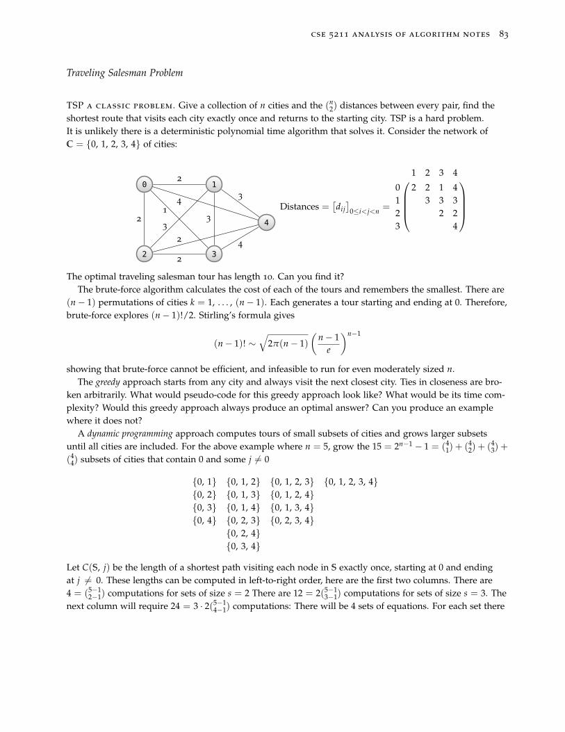
cse 5211 analysis of algorithm notes 83
Traveling Salesman Problem
TSP a classic problem. Give a collection of n cities and the (n2) distances between every pair, find the
shortest route that visits each city exactly once and returns to the starting city. TSP is a hard problem.It is unlikely there is a deterministic polynomial time algorithm that solves it. Consider the network ofC = 0, 1, 2, 3, 4 of cities:
0 1
2 3
4
2
3
4
2
2 3
4
1
3
2
Distances =[dij]
0≤i<j<n =
1 2 3 4
0 2 2 1 41 3 3 32 2 23 4
The optimal traveling salesman tour has length 10. Can you find it?The brute-force algorithm calculates the cost of each of the tours and remembers the smallest. There are
(n− 1) permutations of cities k = 1, . . . , (n− 1). Each generates a tour starting and ending at 0. Therefore,brute-force explores (n− 1)!/2. Stirling’s formula gives
(n− 1)! ∼√
2π(n− 1)(
n− 1e
)n−1
showing that brute-force cannot be efficient, and infeasible to run for even moderately sized n.The greedy approach starts from any city and always visit the next closest city. Ties in closeness are bro-
ken arbitrarily. What would pseudo-code for this greedy approach look like? What would be its time com-plexity? Would this greedy approach always produce an optimal answer? Can you produce an examplewhere it does not?
A dynamic programming approach computes tours of small subsets of cities and grows larger subsetsuntil all cities are included. For the above example where n = 5, grow the 15 = 2n−1 − 1 = (4
1) + (42) + (4
3) +
(44) subsets of cities that contain 0 and some j 6= 0
0, 1 0, 1, 2 0, 1, 2, 3 0, 1, 2, 3, 40, 2 0, 1, 3 0, 1, 2, 40, 3 0, 1, 4 0, 1, 3, 40, 4 0, 2, 3 0, 2, 3, 4
0, 2, 40, 3, 4
Let C(S, j) be the length of a shortest path visiting each node in S exactly once, starting at 0 and endingat j 6= 0. These lengths can be computed in left-to-right order, here are the first two columns. There are4 = (5−1
2−1) computations for sets of size s = 2 There are 12 = 2(5−13−1) computations for sets of size s = 3. The
next column will require 24 = 3 · 2(5−14−1) computations: There will be 4 sets of equations. For each set there
cse 5211 analysis of algorithm notes 84
are 3 cities to end at, and 2 cities to travel through to get to the end.
C(0, 1 , 1) = 2 C(0, 1, 2 , 1) = 5, C(0, 1, 2 , 2) = 5C(0, 2 , 2) = 2 C(0, 1, 3 , 1) = 4, C(0, 1, 3 , 3) = 5C(0, 3 , 3) = 1 C(0, 1, 4 , 1) = 7. C(0, 1, 4 , 4) = 5C(0, 4 , 4) = 4 C(0, 2, 3 , 2) = 3, C(0, 2, 3 , 3) = 4
C(0, 2, 4 , 2) = 6, C(0, 2, 4 , 4) = 4C(0, 3, 4 , 3) = 7, C(0, 3, 4 , 4) = 5
The value of C(S, j) can be expressed in terms of smaller sub-problems.
C(S, j) = mini∈S, i 6=0,j
C(S− j , i) + dij
For instance,
C(0, 1, 2, 3 , 1) = min C(0, 2, 3 , 2) + d21, C(0, 2, 3 , 3) + d31
In general, an optimal path from 0 through S ending at j, is the minimum of a path from 0 through S− jending at i 6= j plus the distance from i to j.
C(S, j) = mini∈S, i 6=0,æ
C(S− 1 , i) + dij
The issue is too many sub-problems.
Here’s some pseudo-code. In line 1 initialize the distances from 0 to every other node. Line 2 starts aloop over all subsets from cardinality s = 3 to n. Line 3 says: Generate all subsets of cardinality s. And, line4 uses the decomposition of paths ending at j into paths ending at i 6= j then moving to j.
1 f o r ( i n t j = 1 ; j < n ; j ++) C(0, j , j) = d0j ; 2 f o r ( i n t s = 3 ; s <= n ; s ++) 3 f o r ( a l l subsets S ⊆ 0, 1, . . . , (n− 1) of s i z e s = |S| conta in ing 0 )
4 f o r ( a l l j ∈ S, j > 0 ) C( S , j ) = min
C(S− j , i) + dij : i ∈ S, i 6= j, i 6= 0
;
5 6 7 return minj C(0, ..., n− 1 , j) + dj0 ;
This leads to a series of equations that can be expressed bottom-up. There are n− 1 = (n−1s−1) initialization
in line 2 where s = 2 is the set cardinality of 0, j , j 6= 0.For sets of cardinality s = 3, there are two sets of equations for paths 0 7→ k 7→ j and 0 7→ j 7→ k
C(0, j, k , j) = C(0, k , k) + dkj for 1 ≤ j < k ≤ n− 1 (20)
C(0, j, k , k) = C(0, j , j) + djk (21)
For the first set, use the summation formula
∑1≤j<k≤(n−1)
1 = ∑1≤j<n−2
∑j+1≤k≤(n−1)
1 = ∑1≤j≤n−2
(n− j− 1) = (n− 2)+ (n− 1)+ · · ·+ 1 =
(n− 1
2
)=
(n− 1s− 1
)The complexity to compute both sets of equations is then
2 · 1 ·(
n− 12
)= (s− 1)(s− 2)
(n− 1s− 1
)
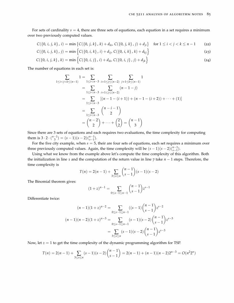
cse 5211 analysis of algorithm notes 85
For sets of cardinality s = 4, there are three sets of equations, each equation in a set requires a minimumover two previously computed values.
C(0, i, j, k , i) = min
C(0, j, k , k) + dki, C(0, j, k , j) + dji
for 1 ≤ i < j < k ≤ n− 1 (22)
C(0, i, j, k , j) = min
C(0, i, k , i) + dij, C(0, i, k , k) + dkj
(23)
C(0, i, j, k , k) = min
C(0, i, j , i) + dik, C(0, i, j , j) + djk
(24)
The number of equations in each set is:
∑1≤i<j<k≤(n−1)
1 = ∑1≤i<n−3
∑i+1≤j≤(n−2)
∑j+1≤k≤(n−1)
1
= ∑1≤i<n−3
∑i+1≤j≤(n−2)
(n− 1− j)
= ∑1≤i<n−3
[(n− 1− (i + 1)) + (n− 1− (i + 2)) + · · ·+ (1)]
= ∑1≤i<n−3
(n− i− 1
2
)=
(n− 2
2
)+ · · ·+
(22
)=
(n− 1
3
)Since there are 3 sets of equations and each requires two evaluations, the time complexity for computingthem is 3 · 2 · (n−1
3 ) = (s− 1)(s− 2)(n−1s−1).
For the five city example, when s = 5, their are four sets of equations, each set requires a minimum overthree previously computed values. Again, the time complexity will be (s− 1)(s− 2)(n−1
s−1).Using what we know from the example above let’s compute the time complexity of this algorithm. Both
the initialization in line 1 and the computation of the return value in line 7 take n− 1 steps. Therefore, thetime complexity is
T(n) = 2(n− 1) + ∑3≤s≤n
(n− 1s− 1
)(s− 1)(s− 2)
The Binomial theorem gives:
(1 + z)n−1 = ∑0≤s−1≤n−1
(n− 1s− 1
)zs−1
Differentiate twice:
(n− 1)(1 + z)n−2 = ∑0≤s−1≤n−1
((s− 1)(
n− 1s− 1
)zs−2
(n− 1)(n− 2)(1 + z)n−3 = ∑0≤s−1≤n−1
(s− 1)(s− 2)(
n− 1s− 1
)zs−3
= ∑3≤s≤n
(s− 1)(s− 2)(
n− 1s− 1
)zs−3
Now, let z = 1 to get the time complexity of the dynamic programming algorithm for TSP.
T(n) = 2(n− 1) + ∑3≤s≤n
(s− 1)(s− 2)(
n− 1s− 1
)= 2(n− 1) + (n− 1)(n− 2)2n−3 = O(n22n)

cse 5211 analysis of algorithm notes 86
Matrix Chain Multiplication
The Matrix Chain Multiplication Problem (MCMP) can be described as a function problem: Find the paren-thesization of a matrix product
M0M1 · · ·Mn−1
to minimize the number of multiply and addition operations. Using a bound B > 0, the MCM decisionproblem asks: Does a given way to parenthesize M0M1 · · ·Mn−1 exist to that uses B or fewer operations?
The number of ways to insert balanced parentheses into a matrix product M0M1 · · ·Mn−1 is the Catalannumber Cn−1. For instance, parentheses can be place in M0M1M2M3 in C3 = 5 ways:
(M0M1)(M2M3), ((M0M1)M2)M3, (M0(M1M2))M3 M0((M1M2)M3), M0(M1(M2M3))
Recall, Cn = (2nn )/(n + 1), grows quickly, so a brute-force search is not feasible for large n.
Inner Products
The matrix product AB = C is the inner product of each row in A with each column in B.
1 innerProduct : : Num a => [ a ] −> [ a ] −> Maybe a2 innerProduct [ ] ys = Nothing3 innerProduct xs [ ] = Nothing4 innerProduct ( x : xs ) ( y : ys ) = x * y + innerProduct xs ys5
6 matrixMult : : Num a => [ [ a ] ] −> [ [ a ] ] −> [ [ a ] ]7 matrixMult xs ys = [ [ ( innerProduct x y ) | y <− ys ] | x <−xs ]
When A is n×m and B is m× p there are np inner products and each inner product requires m multiplica-tions and m− 1 additions.
C[i, j] = ∑0≤k<m
A[i, k]B[k, j], 0 ≤ i < n, 0 ≤ j < p
Therefore the time complexity of the basic matrix multiply algorithm is O(nmp) multiplications and addi-tions.
To see that multiplication order really does matter, consider this example:
M0 has dimensions 10× 100, M1 has dimensions 100× 5, M2 has dimensions 5× 50
There 2 ways to compute the product M0M1M2:
((M0 ×M1)×M2) Cost: (10 · 100 · 5) + (10 · 5 · 50) = 7500
(M0 × (M1 ×M2)) Cost: (100 · 5 · 50) + (10 · 100 · 50) = 75000
Structure of the Optimal Parenthesization
Pretend you want to optimally compute M0M1 · · ·Mn−1 where Mk is a pk × pk+1 matrix. Let
d(i, j) = optimal cost to compute the product Mi · · ·Mj
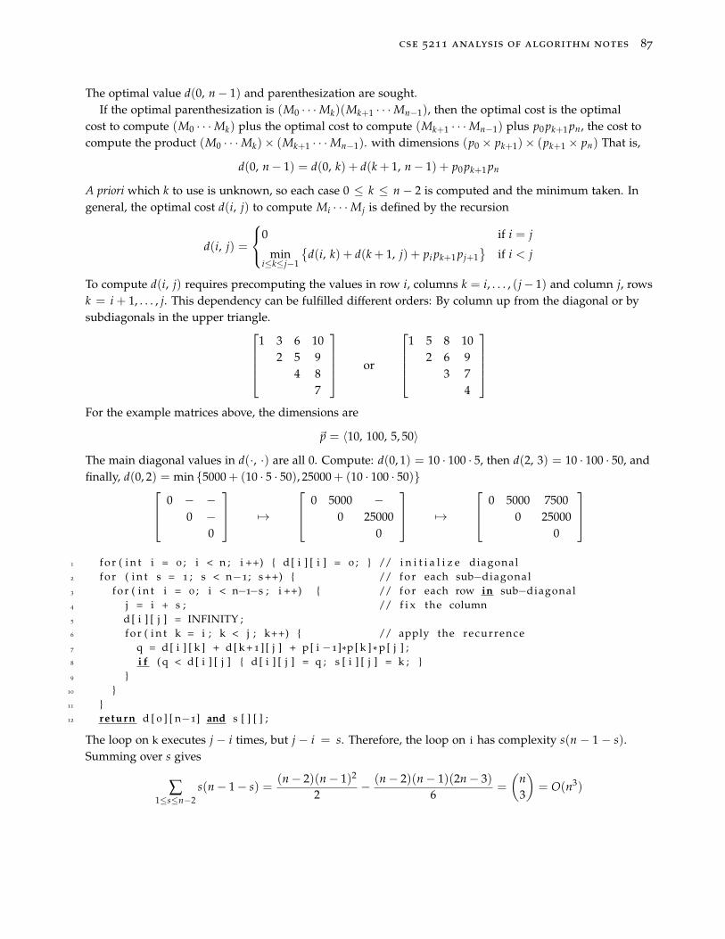
cse 5211 analysis of algorithm notes 87
The optimal value d(0, n− 1) and parenthesization are sought.If the optimal parenthesization is (M0 · · ·Mk)(Mk+1 · · ·Mn−1), then the optimal cost is the optimal
cost to compute (M0 · · ·Mk) plus the optimal cost to compute (Mk+1 · · ·Mn−1) plus p0 pk+1 pn, the cost tocompute the product (M0 · · ·Mk)× (Mk+1 · · ·Mn−1). with dimensions (p0 × pk+1)× (pk+1 × pn) That is,
d(0, n− 1) = d(0, k) + d(k + 1, n− 1) + p0 pk+1 pn
A priori which k to use is unknown, so each case 0 ≤ k ≤ n− 2 is computed and the minimum taken. Ingeneral, the optimal cost d(i, j) to compute Mi · · ·Mj is defined by the recursion
d(i, j) =
0 if i = j
mini≤k≤j−1
d(i, k) + d(k + 1, j) + pi pk+1 pj+1
if i < j
To compute d(i, j) requires precomputing the values in row i, columns k = i, . . . , (j− 1) and column j, rowsk = i + 1, . . . , j. This dependency can be fulfilled different orders: By column up from the diagonal or bysubdiagonals in the upper triangle.
1 3 6 102 5 9
4 87
or
1 5 8 10
2 6 93 7
4
For the example matrices above, the dimensions are
~p = 〈10, 100, 5, 50〉
The main diagonal values in d(·, ·) are all 0. Compute: d(0, 1) = 10 · 100 · 5, then d(2, 3) = 10 · 100 · 50, andfinally, d(0, 2) = min 5000 + (10 · 5 · 50), 25000 + (10 · 100 · 50) 0 − −
0 −0
7→
0 5000 −0 25000
0
7→
0 5000 75000 25000
0
1 f o r ( i n t i = 0 ; i < n ; i ++) d [ i ] [ i ] = 0 ; // i n i t i a l i z e diagonal2 f o r ( i n t s = 1 ; s < n−1; s ++) // f o r each sub−diagonal3 f o r ( i n t i = 0 ; i < n−1−s ; i ++) // f o r each row in sub−diagonal4 j = i + s ; // f i x the column5 d [ i ] [ j ] = INFINITY ;6 f o r ( i n t k = i ; k < j ; k++) // apply the recurrence7 q = d [ i ] [ k ] + d [ k + 1 ] [ j ] + p [ i −1]*p [ k ] * p [ j ] ;8 i f ( q < d [ i ] [ j ] d [ i ] [ j ] = q ; s [ i ] [ j ] = k ; 9
10 11 12 return d [ 0 ] [ n−1] and s [ ] [ ] ;
The loop on k executes j − i times, but j − i = s. Therefore, the loop on i has complexity s(n − 1 − s).Summing over s gives
∑1≤s≤n−2
s(n− 1− s) =(n− 2)(n− 1)2
2− (n− 2)(n− 1)(2n− 3)
6=
(n3
)= O(n3)
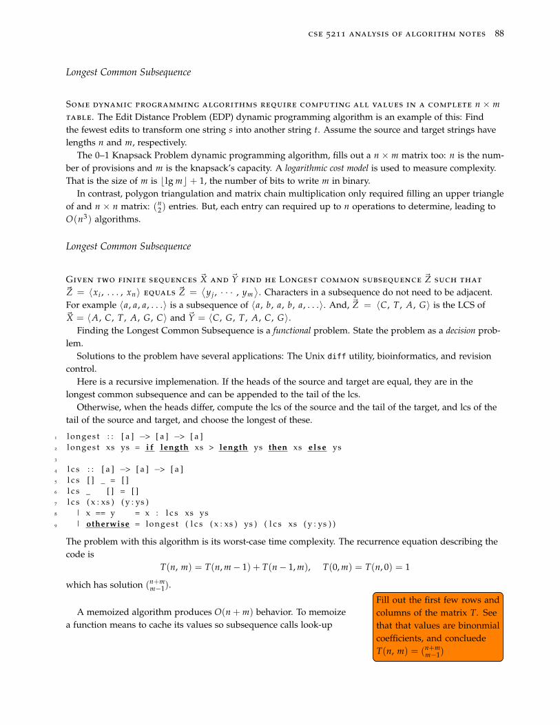
cse 5211 analysis of algorithm notes 88
Longest Common Subsequence
Some dynamic programming algorithms require computing all values in a complete n × mtable. The Edit Distance Problem (EDP) dynamic programming algorithm is an example of this: Findthe fewest edits to transform one string s into another string t. Assume the source and target strings havelengths n and m, respectively.
The 0–1 Knapsack Problem dynamic programming algorithm, fills out a n × m matrix too: n is the num-ber of provisions and m is the knapsack’s capacity. A logarithmic cost model is used to measure complexity.That is the size of m is blg mc + 1, the number of bits to write m in binary.
In contrast, polygon triangulation and matrix chain multiplication only required filling an upper triangleof and n × n matrix: (n
2) entries. But, each entry can required up to n operations to determine, leading toO(n3) algorithms.
Longest Common Subsequence
Given two finite sequences ~X and ~Y find he Longest common subsequence ~Z such that
~Z = 〈xi , . . . , xn〉 equals ~Z =⟨
y j , · · · , ym⟩
. Characters in a subsequence do not need to be adjacent.For example 〈a, a, a, . . .〉 is a subsequence of 〈a, b, a, b, a, . . .〉. And, ~Z = 〈C, T , A, G〉 is the LCS of~X = 〈A, C, T , A, G, C〉 and ~Y = 〈C, G, T , A, C, G〉.
Finding the Longest Common Subsequence is a functional problem. State the problem as a decision prob-lem.
Solutions to the problem have several applications: The Unix diff utility, bioinformatics, and revisioncontrol.
Here is a recursive implemenation. If the heads of the source and target are equal, they are in thelongest common subsequence and can be appended to the tail of the lcs.
Otherwise, when the heads differ, compute the lcs of the source and the tail of the target, and lcs of thetail of the source and target, and choose the longest of these.
1 longes t : : [ a ] −> [ a ] −> [ a ]2 longes t xs ys = i f length xs > length ys then xs e lse ys3
4 l c s : : [ a ] −> [ a ] −> [ a ]5 l c s [ ] _ = [ ]6 l c s _ [ ] = [ ]7 l c s ( x : xs ) ( y : ys )8 | x == y = x : l c s xs ys9 | otherwise = longes t ( l c s ( x : xs ) ys ) ( l c s xs ( y : ys ) )
The problem with this algorithm is its worst-case time complexity. The recurrence equation describing thecode is
T(n, m) = T(n, m− 1) + T(n− 1, m), T(0, m) = T(n, 0) = 1
which has solution (n+mm−1).
Fill out the first few rows andcolumns of the matrix T. Seethat that values are binonmialcoefficients, and concluedeT(n, m) = (n+m
m−1)
Fill out the first few rows andcolumns of the matrix T. Seethat that values are binonmialcoefficients, and concluedeT(n, m) = (n+m
m−1)
A memoized algorithm produces O(n + m) behavior. To memoizea function means to cache its values so subsequence calls look-up

cse 5211 analysis of algorithm notes 89
values instead of recomputing them. The dynamic programmingmachinery behind this can be hidden in a Haskell memoizer. For theData.MemoCombinators memoizer, look-up cost is O(m) where m is thelength of the search string.
1 import qual i f ied Data . MemoCombinators as M2
3 l c s = memoize lcsm4 where5 lcsm [ ] _ = [ ]6 lcsm _ [ ] = [ ]7 lcsm ( x : xs ) ( y : ys )8 | x == y = x : l c s xs ys9 | otherwise = maxl ( l c s ( x : xs ) ys ) ( l c s xs ( y : ys ) )
10
11 maxl x y = i f length x > length y then x e lse y12 memoize = M. memo2 mString mString13 mString = M. l i s t M. char −−Chars the type can be customized for other applications
The worst-case time complexity of this dynamic programming implementation is
T(n, m) = n + m− 1 + (n− 1 + m) = 2(n + m− 1)
Longest common subsequence can be build from the last values in two sequence, too.
1. If ~X and ~Y have the same last element, then the longest common subsequence (LCS) of ~X and ~Y is theLCS of init ~X and init ~Y plus 1.
2. If ~X and ~Y do not end with the same element, then the LCS of ~X and ~Y is the LCS of ~X and init ~Y or theLCS of init ~X and ~Y. whichever is longest.
Let c(i, j) be the length of the longest common subsequence of ~Xi = 〈x0, x1, . . . , xi〉 with ~Yj =⟨y0, y1, . . . , yj
⟩,
then c(i, j) can be defined recursively.
c (i, j) =
0 if i = −1 or j = −1
c (i− 1, j− 1) + 1 if xi = yj
max c (i, j− 1) , c (i− 1, j) if xi 6= yj
Since c (i, j− 1) could equal c (i− 1, j) there can be multiple solutions.
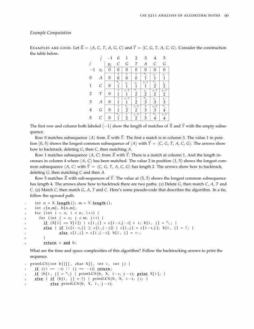
cse 5211 analysis of algorithm notes 90
Example Computation
Examples are good. Let ~X = 〈A, C, T, A, G, C〉 and ~Y = 〈C, G, T, A, C, G〉. Consider the constructionthe table below.
j −1 0 1 2 3 4 5i yj C G T A C G−1 xi 0 0 0 0 0 0 0
0 A 0↑0
↑0
↑0
1
←1
←1
1 C 01
←1
←1
←↑1
2
←2
2 T 0↑1
←↑1
2
←2
←↑2
←↑2
3 A 0↑1
←↑1
↑2
3
←3
←3
4 G 0↑1
2
←↑2
↑3
←↑3
4
5 C 01
↑2
←↑2
↑3
4
←↑4
The first row and column both labeled (−1) show the length of matches of ~X and ~Y with the empty subse-quence.
Row 0 matches subsequence 〈A〉 from ~X with ~Y. The first a match is in column 3. The value 1 in posi-tion (0, 5) shows the longest common subsequence of 〈A〉 with ~Y = 〈C, G, T, A, C, G〉. The arrows showhow to backtrack, deleting G, then C, then matching A.
Row 1 matches subsequence 〈A, C〉 from ~X with ~Y. There is a match at column 1. And the length in-creases in column 4 where 〈A, C〉 has been matched. The value 2 in position (1, 5) shows the longest com-mon subsequence 〈A, C〉 with ~Y = 〈C, G, T, A, C, G〉 has length 2. The arrows show how to backtrack,deleting G, then matching C and then A.
Row 5 matches ~X with sub-sequences of ~Y. The value at (5, 5) shows the longest common subsequencehas length 4. The arrows show how to backtrack there are two paths: (1) Delete G, then match C, A, T andC. (2) Match C, then match G, A, T and C. Here’s some pseudo-code that describes the algorithm. In a tie,follow the upward path.
1 i n t n = X . length ( ) ; m = Y . length ( ) ;2 i n t c [ n ,m] , b [ n ,m] ;3 f o r ( i n t i = 0 ; i < n ; i ++) 4 f o r ( i n t j = 0 ; j < m; j ++) 5 i f (X[ i ] == Y[ i ] ) c [ i , j ] = c [ i −1 , j −1] + 1 ; b [ i , j ] = ; 6 e lse i f ( c [ i −1 , j ] ≥ c [ i , j −1]) c [ i , j ] = c [ i −1 , j ] ; b [ i , j ] = ↑ ; 7 e lse c [ i , j ] = c [ i , j −1] ; b [ i , j ] = ← ;8 9 return c and b ;
What are the time and space complexities of this algorithm? Follow the backtracking arrows to print thesequence.
1 printLCS ( i n t b [ ] [ ] , char X [ ] , i n t i , i n t j ) 2 i f ( ( i == −1) || ( j == −1)) return ;3 i f ( b [ i , j ] = ) printLCS ( b , X , i −1 , j −1) ; print X[ i ] ; 4 e lse i f ( b [ i , j ] = ↑ ) printLCS ( b , X , i −1 , j ) ; 5 e lse printLCS ( b , X , i , j −1) ;
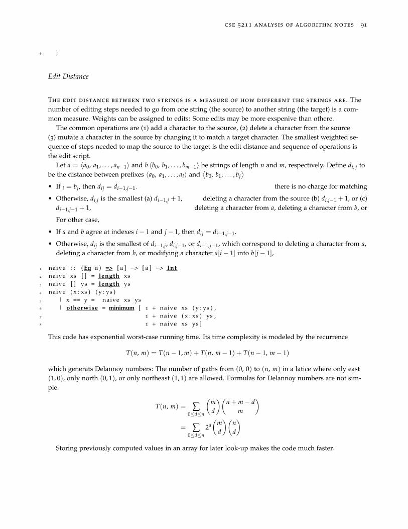
cse 5211 analysis of algorithm notes 91
6
Edit Distance
The edit distance between two strings is a measure of how different the strings are. Thenumber of editing steps needed to go from one string (the source) to another string (the target) is a com-mon measure. Weights can be assigned to edits: Some edits may be more exspenive than othere.
The common operations are (1) add a character to the source, (2) delete a character from the source(3) mutate a character in the source by changing it to match a target character. The smallest weighted se-quence of steps needed to map the source to the target is the edit distance and sequence of operations isthe edit script.
Let a = 〈a0, a1, . . . , an−1〉 and b 〈b0, b1, . . . , bm−1〉 be strings of length n and m, respectively. Define di, j tobe the distance between prefixes 〈a0, a1, . . . , ai〉 and
⟨b0, b1, . . . , bj
⟩• If i = bj, then dij = di−1,j−1. there is no charge for matching
• Otherwise, di,j is the smallest (a) di−1,j + 1, deleting a character from the source (b) di,j−1 + 1, or (c)di−1,j−1 + 1, deleting a character from a, deleting a character from b, or
For other case,
• If a and b agree at indexes i− 1 and j− 1, then dij = di−1,j−1.
• Otherwise, dij is the smallest of di−1,j, di,j−1, or di−1,j−1, which correspond to deleting a character from a,deleting a character from b, or modifying a character a[i− 1] into b[j− 1],
1 naive : : ( Eq a ) => [ a ] −> [ a ] −> Int2 naive xs [ ] = length xs3 naive [ ] ys = length ys4 naive ( x : xs ) ( y : ys )5 | x == y = naive xs ys6 | otherwise = minimum [ 1 + naive xs ( y : ys ) ,7 1 + naive ( x : xs ) ys ,8 1 + naive xs ys ]
This code has exponential worst-case running time. Its time complexity is modeled by the recurrence
T(n, m) = T(n− 1, m) + T(n, m− 1) + T(n− 1, m− 1)
which generats Delannoy numbers: The number of paths from (0, 0) to (n, m) in a latice where only east(1, 0), only north (0, 1), or only northeast (1, 1) are allowed. Formulas for Delannoy numbers are not sim-ple.
T(n, m) = ∑0≤d≤n
(md
)(n + m− d
m
)= ∑
0≤d≤n2d(
md
)(nd
)Storing previously computed values in an array for later look-up makes the code much faster.
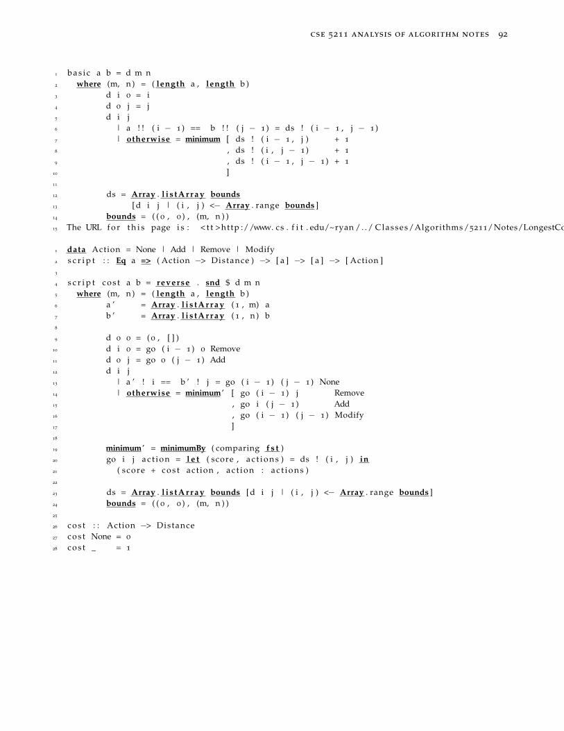
cse 5211 analysis of algorithm notes 92
1 b a s i c a b = d m n2 where (m, n ) = ( length a , length b )3 d i 0 = i4 d 0 j = j5 d i j6 | a ! ! ( i − 1 ) == b ! ! ( j − 1 ) = ds ! ( i − 1 , j − 1 )7 | otherwise = minimum [ ds ! ( i − 1 , j ) + 1
8 , ds ! ( i , j − 1 ) + 1
9 , ds ! ( i − 1 , j − 1 ) + 1
10 ]11
12 ds = Array . l i s t A r r a y bounds13 [ d i j | ( i , j ) <− Array . range bounds ]14 bounds = ( ( 0 , 0 ) , (m, n ) )15 The URL f o r t h i s page i s : < t t >http ://www. cs . f i t . edu/~ryan / . . / Classes/Algorithms /5211/Notes/LongestCommonSubsequence . tex </ t t ><br>
1 data Action = None | Add | Remove | Modify2 s c r i p t : : Eq a => ( Action −> Distance ) −> [ a ] −> [ a ] −> [ Action ]3
4 s c r i p t c o s t a b = reverse . snd $ d m n5 where (m, n ) = ( length a , length b )6 a ’ = Array . l i s t A r r a y ( 1 , m) a7 b ’ = Array . l i s t A r r a y ( 1 , n ) b8
9 d 0 0 = ( 0 , [ ] )10 d i 0 = go ( i − 1 ) 0 Remove11 d 0 j = go 0 ( j − 1 ) Add12 d i j13 | a ’ ! i == b ’ ! j = go ( i − 1 ) ( j − 1 ) None14 | otherwise = minimum’ [ go ( i − 1 ) j Remove15 , go i ( j − 1 ) Add16 , go ( i − 1 ) ( j − 1 ) Modify17 ]18
19 minimum’ = minimumBy ( comparing f s t )20 go i j a c t i o n = l e t ( score , a c t i o n s ) = ds ! ( i , j ) in21 ( score + c o s t act ion , a c t i o n : a c t i o n s )22
23 ds = Array . l i s t A r r a y bounds [ d i j | ( i , j ) <− Array . range bounds ]24 bounds = ( ( 0 , 0 ) , (m, n ) )25
26 c o s t : : Action −> Distance27 c o s t None = 0
28 c o s t _ = 1
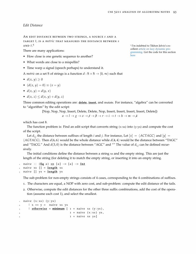
cse 5211 analysis of algorithm notes 93
Edit Distance
An edit distance between two strings, a source s and a
target t, is a metric that measures the distance between sand t.5 5 I’m indebted to Tikhon Jelvis’s ex-
cellent article on lazy dynamic pro-gramming. Get the code for this sectionhere
There are many applications:
• How close is one genetic sequence to another?
• What words are close to a mispellin?
• Time warp a signal (speech perhaps) to understand it.
A metric on a set S of strings is a function d : S× S→ [0, ∞) such that
• d(x, y) ≥ 0
• (d(x, y) = 0) ≡ (x = y)
• d(x, y) = d(y, x)
• d(x, z) ≤ d(x, y) + d(y, z)
Three common editing operations are: delete, insert, and mutate. For instance, “algebra” can be convertedto “algorithm” by the edit script:
[Nop, Nop, Nop, Insert, Delete, Delete, Nop, Insert, Insert, Insert, Insert, Delete])a→ l → g→ o →6 e→6 b→ r → i→ t→ h→ m→6 a
which has cost 8.The function problem is: Find an edit script that converts string (x:xs) into (y:ys) and compute the cost
of the script.Let di,j the distance between suffixes of length i and j. For instance, Let [x] = 〈ACTAGC〉 and [y] =
〈AGTACG〉. Then d(6, 6) would be the whole distance while d(4, 4) would be the distance between “TAGC”and “TACG.” And d(3, 0) is the distance between “AGC” and “” The value of di,j can be defined recur-sively.
The initial conditions define the distance between a string xs and the empty string. This are just thelength of the string (for deleting it to match the empty string, or inserting it into an empty string.
1 naive : : ( Eq a ) => [ a ] −> [ a ] −> Int2 naive xs [ ] = length xs −− delete xs to match the empty string3 naive [ ] ys = length ys −− insert ys in to the empty string
The sub-problem for non-empty strings consists of 4 cases, corresponding to the 4 combinations of suffixes.
1. The characters are equal, a NOP with zero cost, and sub-problem: compute the edit distance of the tails.
2. Otherwise, compute the edit distances for the other three suffix combinations, add the cost of the opera-tion (assume each cost 1), and select the smallest.
1 naive ( x : xs ) ( y : ys )2 | x == y = naive xs ys3 | otherwise = minimum [ 1 + naive xs ( y : ys ) ,4 1 + naive ( x : xs ) ys ,5 1 + naive xs ys ]
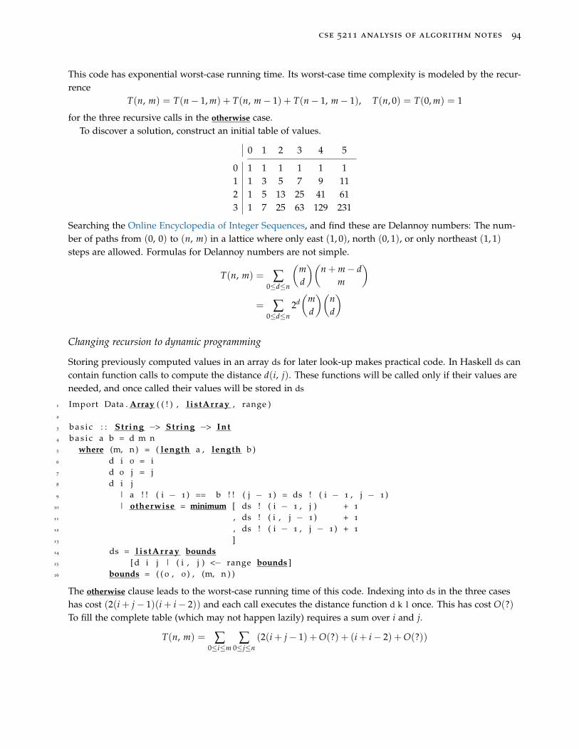
cse 5211 analysis of algorithm notes 94
This code has exponential worst-case running time. Its worst-case time complexity is modeled by the recur-rence
T(n, m) = T(n− 1, m) + T(n, m− 1) + T(n− 1, m− 1), T(n, 0) = T(0, m) = 1
for the three recursive calls in the otherwise case.To discover a solution, construct an initial table of values.
0 1 2 3 4 5
0 1 1 1 1 1 11 1 3 5 7 9 112 1 5 13 25 41 613 1 7 25 63 129 231
Searching the Online Encyclopedia of Integer Sequences, and find these are Delannoy numbers: The num-ber of paths from (0, 0) to (n, m) in a lattice where only east (1, 0), north (0, 1), or only northeast (1, 1)steps are allowed. Formulas for Delannoy numbers are not simple.
T(n, m) = ∑0≤d≤n
(md
)(n + m− d
m
)= ∑
0≤d≤n2d(
md
)(nd
)
Changing recursion to dynamic programming
Storing previously computed values in an array ds for later look-up makes practical code. In Haskell ds cancontain function calls to compute the distance d(i, j). These functions will be called only if their values areneeded, and once called their values will be stored in ds
1 Import Data . Array ( ( ! ) , l i s tArray , range )2
3 b a s i c : : String −> String −> Int4 b a s i c a b = d m n5 where (m, n ) = ( length a , length b )6 d i 0 = i7 d 0 j = j8 d i j9 | a ! ! ( i − 1 ) == b ! ! ( j − 1 ) = ds ! ( i − 1 , j − 1 )
10 | otherwise = minimum [ ds ! ( i − 1 , j ) + 1
11 , ds ! ( i , j − 1 ) + 1
12 , ds ! ( i − 1 , j − 1 ) + 1
13 ]14 ds = l i s t A r r a y bounds15 [ d i j | ( i , j ) <− range bounds ]16 bounds = ( ( 0 , 0 ) , (m, n ) )
The otherwise clause leads to the worst-case running time of this code. Indexing into ds in the three caseshas cost (2(i + j− 1)(i + i− 2)) and each call executes the distance function d k l once. This has cost O(?)To fill the complete table (which may not happen lazily) requires a sum over i and j.
T(n, m) = ∑0≤i≤m
∑0≤j≤n
(2(i + j− 1) + O(?) + (i + i− 2) + O(?))
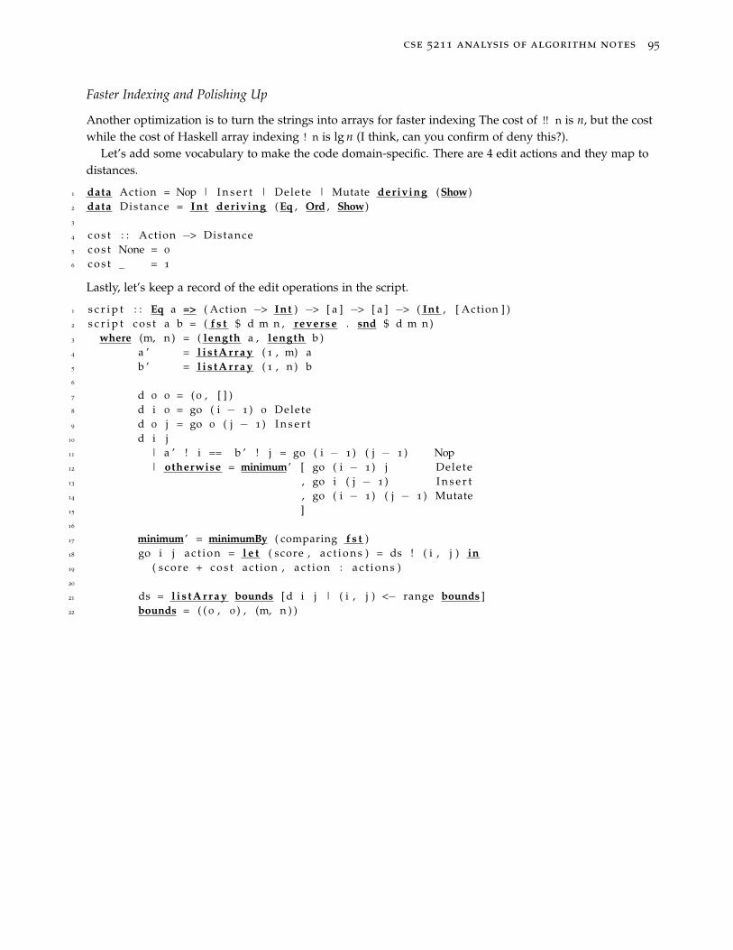
cse 5211 analysis of algorithm notes 95
Faster Indexing and Polishing Up
Another optimization is to turn the strings into arrays for faster indexing The cost of !! n is n, but the costwhile the cost of Haskell array indexing ! n is lg n (I think, can you confirm of deny this?).
Let’s add some vocabulary to make the code domain-specific. There are 4 edit actions and they map todistances.
1 data Action = Nop | I n s e r t | Delete | Mutate deriving (Show)2 data Distance = Int deriving ( Eq , Ord , Show)3
4 c o s t : : Action −> Distance5 c o s t None = 0
6 c o s t _ = 1
Lastly, let’s keep a record of the edit operations in the script.
1 s c r i p t : : Eq a => ( Action −> Int ) −> [ a ] −> [ a ] −> ( Int , [ Action ] )2 s c r i p t c o s t a b = ( f s t $ d m n , reverse . snd $ d m n )3 where (m, n ) = ( length a , length b )4 a ’ = l i s t A r r a y ( 1 , m) a5 b ’ = l i s t A r r a y ( 1 , n ) b6
7 d 0 0 = ( 0 , [ ] )8 d i 0 = go ( i − 1 ) 0 Delete9 d 0 j = go 0 ( j − 1 ) I n s e r t
10 d i j11 | a ’ ! i == b ’ ! j = go ( i − 1 ) ( j − 1 ) Nop12 | otherwise = minimum’ [ go ( i − 1 ) j Delete13 , go i ( j − 1 ) I n s e r t14 , go ( i − 1 ) ( j − 1 ) Mutate15 ]16
17 minimum’ = minimumBy ( comparing f s t )18 go i j a c t i o n = l e t ( score , a c t i o n s ) = ds ! ( i , j ) in19 ( score + c o s t act ion , a c t i o n : a c t i o n s )20
21 ds = l i s t A r r a y bounds [ d i j | ( i , j ) <− range bounds ]22 bounds = ( ( 0 , 0 ) , (m, n ) )

cse 5211 analysis of algorithm notes 96
Graph Algorithms
Graphs are useful and interesting. Many problems can be modeled by a graph G = (V, E).
Trees
Trees are special! They have a recursive description. For instance, a binary Tree holding data of type a
can be defined as:
1 data Tree a = Empty | Node a ( Tree a ) ( Tree a ) deriving (Show)
There are three basic traversals of a binary tree.
1. Preorder traversal: Visit where you are, then go left, then right.
1 preorder : : Tree a −> [ a ]2 preorder Empty = [ ]3 preorder (Node root l e f t r i g h t ) = root : ( preorder l e f t ) ++ ( preorder r i g h t )
Preorder traversal on a binary tree is a special case of depth-first search.
2. Inorder traversal: Go left, then home to the root, then right.
1 inorder : : Tree a −> [ a ]2 inorder Empty = [ ]3 inorder (Node root l e f t r i g h t ) = inorder l e f t ++ ( root : inorder r i g h t )
3. Postorder traversal: Go left, go right, then visit the root.
1 postorder : : Tree a −> [ a ]2 postorder Empty = [ ]3 postorder (Node root l e f t r i g h t ) = postorder l e f t ++ postorder r i g h t ++ [ root ]
To analyze these tree traversal, assume there are n nodes in a tree. Then the time complexity of preordercan be modeled by the equation
T(n) = 1 + T(k) + T(n− k− 1) + (k + 1)
where for a given k = 0, . . . , n− 1, k is the number of nodes in the left subtree and (n− k− 1) counts thenodes in the right subtree The term (k + 1) is the concatenation cost.
In the worst case k = n− 1 the recursion is
T(n) = 1 + T(n− 1) + n
and its time complexity is O(n2).
Postorder tranversal is the converse of preoder: Descendants occur before ancestors and left subtreesbefore right subtrees.
Trees can be defined recursively. Algorithms on trees map natually to functional descriptions. Unfortu-nately, graphs in general, have no recursive structure.
• A node can have any number of children for a node.
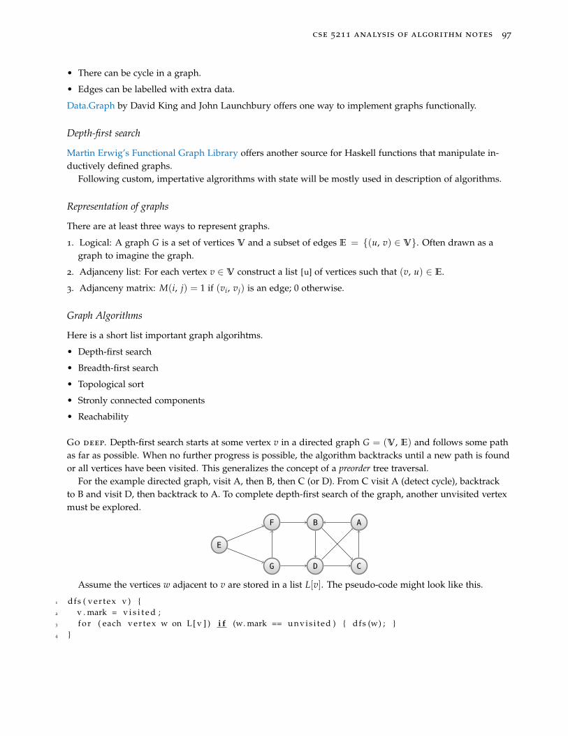
cse 5211 analysis of algorithm notes 97
• There can be cycle in a graph.
• Edges can be labelled with extra data.
Data.Graph by David King and John Launchbury offers one way to implement graphs functionally.
Depth-first search
Martin Erwig’s Functional Graph Library offers another source for Haskell functions that manipulate in-ductively defined graphs.
Following custom, impertative algrorithms with state will be mostly used in description of algorithms.
Representation of graphs
There are at least three ways to represent graphs.
1. Logical: A graph G is a set of vertices V and a subset of edges E = (u, v) ∈ V. Often drawn as agraph to imagine the graph.
2. Adjanceny list: For each vertex v ∈ V construct a list [u] of vertices such that (v, u) ∈ E.
3. Adjanceny matrix: M(i, j) = 1 if (vi, vj) is an edge; 0 otherwise.
Graph Algorithms
Here is a short list important graph algorihtms.
• Depth-first search
• Breadth-first search
• Topological sort
• Stronly connected components
• Reachability
Go deep. Depth-first search starts at some vertex v in a directed graph G = (V, E) and follows some pathas far as possible. When no further progress is possible, the algorithm backtracks until a new path is foundor all vertices have been visited. This generalizes the concept of a preorder tree traversal.
For the example directed graph, visit A, then B, then C (or D). From C visit A (detect cycle), backtrackto B and visit D, then backtrack to A. To complete depth-first search of the graph, another unvisited vertexmust be explored.
AB
CD
F
G
E
Assume the vertices w adjacent to v are stored in a list L[v]. The pseudo-code might look like this.
1 dfs ( ver tex v ) 2 v . mark = v i s i t e d ;3 f o r ( each ver tex w on L [ v ] ) i f (w. mark == unvis i ted ) dfs (w) ; 4
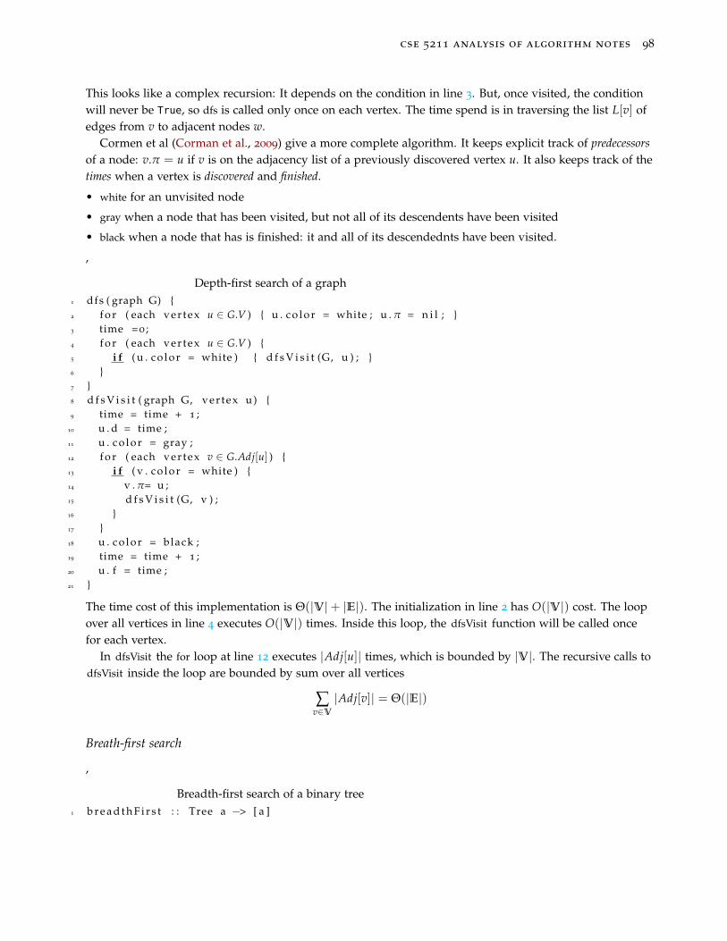
cse 5211 analysis of algorithm notes 98
This looks like a complex recursion: It depends on the condition in line 3. But, once visited, the conditionwill never be True, so dfs is called only once on each vertex. The time spend is in traversing the list L[v] ofedges from v to adjacent nodes w.
Cormen et al (Corman et al., 2009) give a more complete algorithm. It keeps explicit track of predecessorsof a node: v.π = u if v is on the adjacency list of a previously discovered vertex u. It also keeps track of thetimes when a vertex is discovered and finished.
• white for an unvisited node
• gray when a node that has been visited, but not all of its descendents have been visited
• black when a node that has is finished: it and all of its descendednts have been visited.
,
Depth-first search of a graph1 dfs ( graph G) 2 f o r ( each ver tex u ∈ G.V ) u . c o l o r = white ; u . π = n i l ; 3 time =0 ;4 f o r ( each ver tex u ∈ G.V ) 5 i f ( u . c o l o r = white ) d f s V i s i t (G, u ) ; 6 7 8 d f s V i s i t ( graph G, ver tex u ) 9 time = time + 1 ;
10 u . d = time ;11 u . c o l o r = gray ;12 f o r ( each ver tex v ∈ G.Adj[u] ) 13 i f ( v . c o l o r = white ) 14 v . π= u ;15 d f s V i s i t (G, v ) ;16 17 18 u . c o l o r = black ;19 time = time + 1 ;20 u . f = time ;21
The time cost of this implementation is Θ(|V|+ |E|). The initialization in line 2 has O(|V|) cost. The loopover all vertices in line 4 executes O(|V|) times. Inside this loop, the dfsVisit function will be called oncefor each vertex.
In dfsVisit the for loop at line 12 executes |Adj[u]| times, which is bounded by |V|. The recursive calls todfsVisit inside the loop are bounded by sum over all vertices
∑v∈V
|Adj[v]| = Θ(|E|)
Breath-first search
,
Breadth-first search of a binary tree1 b r e a d t h F i r s t : : Tree a −> [ a ]
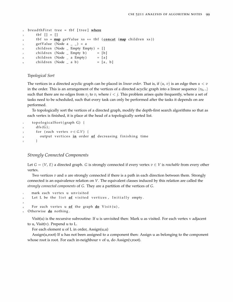
cse 5211 analysis of algorithm notes 99
2 b r e a d t h F i r s t t r e e = t b f [ t r e e ] where3 t b f [ ] = [ ]4 t b f xs = map getValue xs ++ t b f ( concat (map ch i ldren xs ) )5 getValue (Node a _ _ ) = a6 ch i ldren (Node _ Empty Empty ) = [ ]7 ch i ldren (Node _ Empty b ) = [ b ]8 ch i ldren (Node _ a Empty ) = [ a ]9 ch i ldren (Node _ a b ) = [ a , b ]
Topological Sort
The vertices in a directed acyclic graph can be placed in linear order. That is, if (u, v) is an edge then u < vin the order. This is an arrangement of the vertices of a directed acyclic graph into a linear sequence 〈v0, ..〉such that there are no edges from vj to vi where i < j. This problem arises quite frequently, where a set oftasks need to be scheduled, such that every task can only be performed after the tasks it depends on areperformed.
To topologically sort the vertices of a directed graph, modify the depth-first search algorithms so that aseach vertex is finished, it is place at the head of a topologically sorted list.
1 t o p o l o g i c a l S o r t ( graph G) 2 dfs (G) ;3 f o r ( each ver tex v ∈ G.V ) 4 output v e r t i c e s in order of decreas ing f i n i s h i n g time5
Strongly Connected Components
Let G = (V, E) a directed graph. G is strongly connected if every vertex v ∈ V is reachable from every othervertex.
Two vertices v and u are strongly connected if there is a path in each direction between them. Stronglyconnected is an equivalence relation on V. The equivalent classes induced by this relation are called thestrongly connected components of G. They are a partition of the vertices of G.
1 mark each ver tex u unvis i ted2 Let L be the l i s t of v i s i t e d v e r t i c e s , I n i t i a l l y empty .3
4 For each ver tex u of the graph do V i s i t ( u ) ,5 Otherwise do nothing .
Visit(u) is the recursive subroutine: If u is unvisited then: Mark u as visited. For each vertex v adjacentto u, Visit(v). Prepend u to L.
For each element u of L in order, Assign(u,u)Assign(u,root) If u has not been assigned to a component then: Assign u as belonging to the component
whose root is root. For each in-neighbour v of u, do Assign(v,root).

cse 5211 analysis of algorithm notes 100
References
Corman, T. H., Leiserson, C. E., Rivest, R. L., and Stein, C. (2009). Introduction to Algorithms. MIT Press,third edition. [page 98]

cse 5211 analysis of algorithm notes 101
Backtracking Algorithms
Conceptually, backtracking algorithms perform depth-first searches. Backtracking algo-rithms are often used to solve constraint satisfaction problems. Constraints are a set of equations or inequal-ities that must be met. Usually, the set of feasible solutions is large. The goal is to find a feasible solutionthat minimizes or maximizes an objective function.
The Traveling Salesman & Hamiltonian Circuit Problem
A Hamiltonian tour or circuit in an undirected graph G = (E, V) is a cycle that passes through each nodeexactly once. When the edges have non-negative weights, a traveling salesman wants to find the shortesttour. Name the nodes 0 through n − 1. Since the tour is a cycle, the first node is arbitrary, and might aswell be 0. A tour is a permutation of 1, 2, . . . , (n− 1), so there are (n− 1)! possible tours. But, the graph isundirected, so a permutation [0, 1, 2, 3, 4, 5] is equivalent to [0, 5, 4, 3, 2, 1].
0 1
2 3
4
2
3
4
1
2 3
4
1
2
2
A dynamic programming algorithm for TSP was presented previously.Backtracking algorithms usually have a bounding function that allows the search space to be pruned.An adjacency matrix for the above graph is:
Distances =[dij]
0≤i<j<n = M =
0 1 2 3 4
0 ∞ 2 2 1 41 ∞ 2 3 32 ∞ 1 23 ∞ 44 ∞
You can compute the cost of a tour by walking through the graph, for instance 0 7→ 2 7→ 4 7→ 3 7→ 1 7→ 0has cost 2 + 2 + 4 + 3 + 2 = 13. A tour covers all rows and columns: (0, 2), (2, 4), (4, 3), (3, 1), (1, 0)
The adjacency matrix M can be reduced in two steps to create a lower bound on the cost of a tour.
1. First subtract the minimum in each row from itself and other values in the row. Sum the amount sub-tracted.
2. Second, using this intermediate matrix, subtract the minimum in each column from itself and the othervalues in the column. Sum the amount subtracted and add it to the previous sum. Call this value V(M).
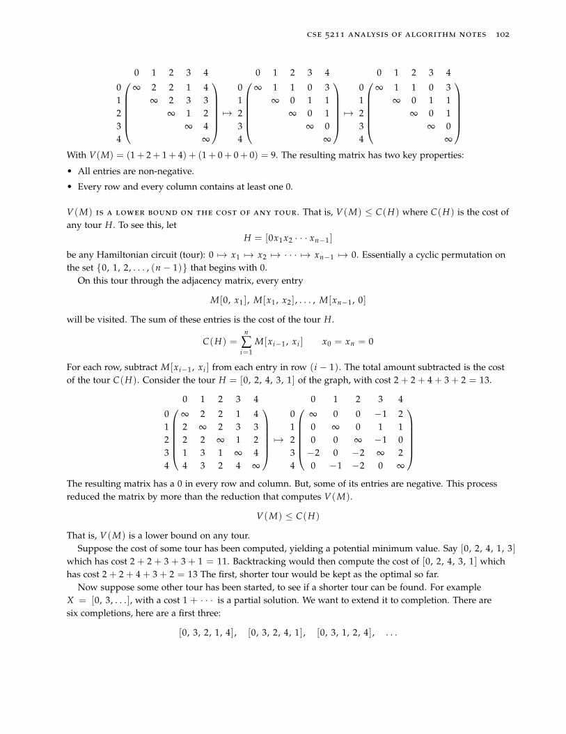
cse 5211 analysis of algorithm notes 102
0 1 2 3 4
0 ∞ 2 2 1 41 ∞ 2 3 32 ∞ 1 23 ∞ 44 ∞
7→
0 1 2 3 4
0 ∞ 1 1 0 31 ∞ 0 1 12 ∞ 0 13 ∞ 04 ∞
7→
0 1 2 3 4
0 ∞ 1 1 0 31 ∞ 0 1 12 ∞ 0 13 ∞ 04 ∞
With V(M) = (1 + 2 + 1 + 4) + (1 + 0 + 0 + 0) = 9. The resulting matrix has two key properties:
• All entries are non-negative.
• Every row and every column contains at least one 0.
V(M) is a lower bound on the cost of any tour. That is, V(M) ≤ C(H) where C(H) is the cost ofany tour H. To see this, let
H = [0x1 x2 · · · xn−1 ]
be any Hamiltonian circuit (tour): 0 7→ x1 7→ x2 7→ · · · 7→ xn−1 7→ 0. Essentially a cyclic permutation onthe set 0, 1, 2, . . . , (n − 1) that begins with 0.
On this tour through the adjacency matrix, every entry
M[0, x1 ], M[x1 , x2 ], . . . , M[xn−1 , 0]
will be visited. The sum of these entries is the cost of the tour H.
C(H) =n
∑i=1
M[xi−1 , xi ] x0 = xn = 0
For each row, subtract M[xi−1 , xi ] from each entry in row (i − 1). The total amount subtracted is the costof the tour C(H). Consider the tour H = [0, 2, 4, 3, 1] of the graph, with cost 2 + 2 + 4 + 3 + 2 = 13.
0 1 2 3 4
0 ∞ 2 2 1 41 2 ∞ 2 3 32 2 2 ∞ 1 23 1 3 1 ∞ 44 4 3 2 4 ∞
7→
0 1 2 3 4
0 ∞ 0 0 −1 21 0 ∞ 0 1 12 0 0 ∞ −1 03 −2 0 −2 ∞ 24 0 −1 −2 0 ∞
The resulting matrix has a 0 in every row and column. But, some of its entries are negative. This processreduced the matrix by more than the reduction that computes V(M).
V(M) ≤ C(H)
That is, V(M) is a lower bound on any tour.Suppose the cost of some tour has been computed, yielding a potential minimum value. Say [0, 2, 4, 1, 3]
which has cost 2 + 2 + 3 + 3 + 1 = 11. Backtracking would then compute the cost of [0, 2, 4, 3, 1] whichhas cost 2 + 2 + 4 + 3 + 2 = 13 The first, shorter tour would be kept as the optimal so far.
Now suppose some other tour has been started, to see if a shorter tour can be found. For exampleX = [0, 3, . . .], with a cost 1 + · · · is a partial solution. We want to extend it to completion. There aresix completions, here are a first three:
[0, 3, 2, 1, 4], [0, 3, 2, 4, 1], [0, 3, 1, 2, 4], . . .
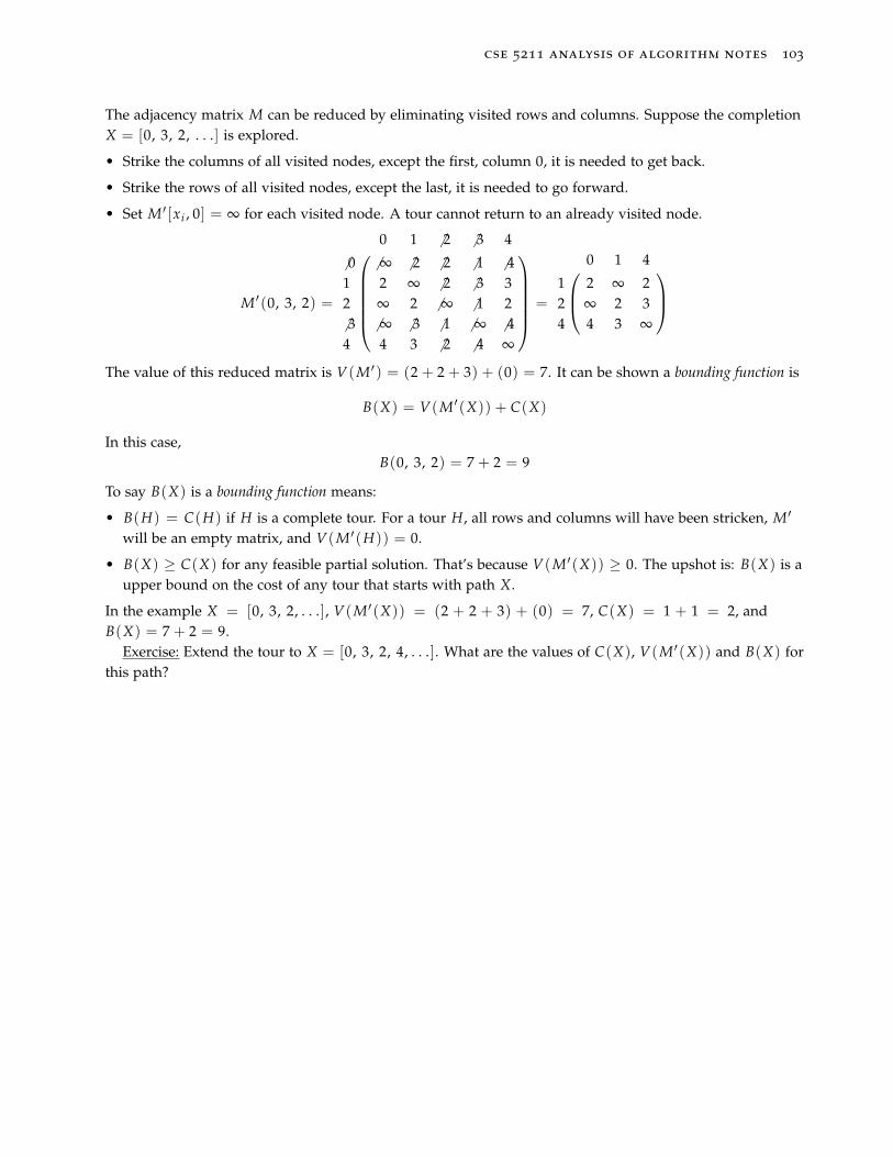
cse 5211 analysis of algorithm notes 103
The adjacency matrix M can be reduced by eliminating visited rows and columns. Suppose the completionX = [0, 3, 2, . . .] is explored.
• Strike the columns of all visited nodes, except the first, column 0, it is needed to get back.
• Strike the rows of all visited nodes, except the last, it is needed to go forward.
• Set M ′ [xi , 0] = ∞ for each visited node. A tour cannot return to an already visited node.
M ′(0, 3, 2) =
0 1 6 2 6 3 4
6 0 6 ∞ 6 2 6 2 6 1 6 41 2 ∞ 6 2 6 3 32 ∞ 2 6 ∞ 6 1 26 3 6 ∞ 6 3 6 1 6 ∞ 6 44 4 3 6 2 6 4 ∞
=
0 1 4
1 2 ∞ 22 ∞ 2 34 4 3 ∞
The value of this reduced matrix is V(M ′) = (2 + 2 + 3) + (0) = 7. It can be shown a bounding function is
B(X) = V(M ′(X)) + C(X)
In this case,B(0, 3, 2) = 7 + 2 = 9
To say B(X) is a bounding function means:
• B(H) = C(H) if H is a complete tour. For a tour H, all rows and columns will have been stricken, M ′
will be an empty matrix, and V(M ′(H)) = 0.
• B(X) ≥ C(X) for any feasible partial solution. That’s because V(M ′(X)) ≥ 0. The upshot is: B(X) is aupper bound on the cost of any tour that starts with path X.
In the example X = [0, 3, 2, . . .], V(M ′(X)) = (2 + 2 + 3) + (0) = 7, C(X) = 1 + 1 = 2, andB(X) = 7 + 2 = 9.
Exercise: Extend the tour to X = [0, 3, 2, 4, . . .]. What are the values of C(X), V(M ′(X)) and B(X) forthis path?

cse 5211 analysis of algorithm notes 104
Backtracking Algorithms, Part 2
Backtracking algorithms can be used to solve constraint satisfaction problems. The 0—1 Knapsack Problemis an example problem that can be solved by backtracking. (There are other approaches (greedy, dynamicprogramming) for this problem.) The Set Partition problem: Can a set integers be partitioned into two non-empty subsets that have equal sums over their values. It is an N P-complete problem. Partition is a specialcase of the Knapsack problem: Assume each items weight equals its value and C = V = 1/2 ∑ weights.Solving Knapsack in this special case solves Partition.
0—1 Knapsack Problem
Given a knapsack with capacity C, and a list of provisions (an inventory) 〈pk : k ∈N〉 (the list could beunbounded) A provision p is a 3–tuple
p :: (String, Num, Num) = (name, weight, value)
Decision Problem: Given a value V, is there a subset I of provisions such that
∑p∈I
pweight ≤ C, and
∑p∈I
pvalue ≥ V
This decision problem is NP-complete.Function Problem: Find the maximum value of V over all feasible subsets of provisions. A subset is fea-
sible if the sum of its weights does not exceed the capacity C of the knapsack. This function problem isNP-hard.
A useful abstraction is to consider both summations to be over the entire inventory (list of provisions).This is accomplished using a a bit vector
〈b0, b1, b2, b3, . . .〉
where a particular bit bk is set to 1 or 0 depending on whether or not provision pk is or is not placed in theknapsack. There are several things this reveals.
• There are 2n bit vectors of length n (or subsets of an n element set Zn = 0, 1, . . . , (n− 1). Exhaustivesearch will take exponential time.
• Not all subsets need to be explored: Once a subset is infeasible so are all of its super-sets.
Here is a functional algorithm for the problem. An example inventory is given. The combs function thatsearches over all combinations of provisions from the inventory (subsets of it). The main function specifiesthe input and output. The Haskell code is from Rosetta Code
The combs function maps a list of provisions and a capacity to and ordered pair: a value and its feasiblelist of provisions.
As an initial condition, if the provision list is empty, then for any capacity, the returned value is 0 andthe empty list.
Given an non-empty list of provisions, there are two possibilities: (1) If the weight of the provision at thehead of the list is less than the capacity, then including the provision is feasible, otherwise (2) the provisioncannot be in a feasible solution.
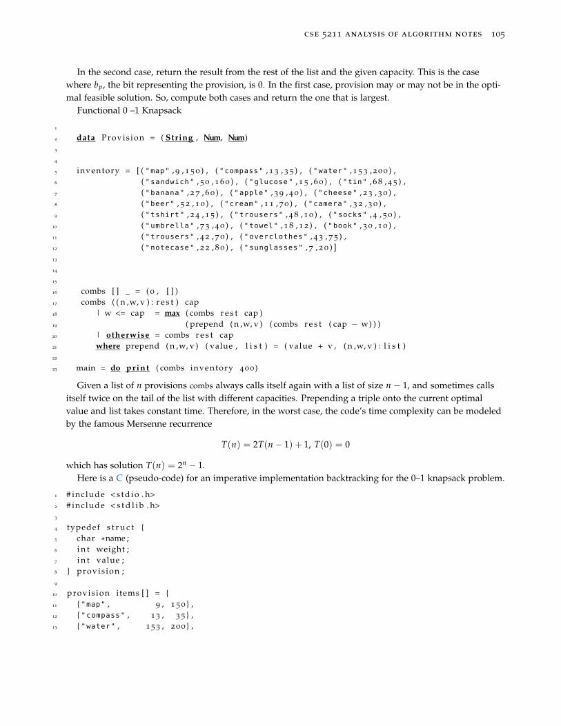
cse 5211 analysis of algorithm notes 105
In the second case, return the result from the rest of the list and the given capacity. This is the casewhere bp, the bit representing the provision, is 0. In the first case, provision may or may not be in the opti-mal feasible solution. So, compute both cases and return the one that is largest.
Functional 0 –1 Knapsack
1 −−A provision is its name, its weight, and its value2 data Provis ion = ( String , Num, Num)3
4 −−Here is a sample inventory of provisions5 inventory = [ ( "map" , 9 , 1 5 0 ) , ( "compass" , 1 3 , 3 5 ) , ( "water" , 1 5 3 , 2 0 0 ) ,6 ( "sandwich" , 5 0 , 1 6 0 ) , ( "glucose" , 1 5 , 6 0 ) , ( "tin" , 6 8 , 4 5 ) ,7 ( "banana" , 2 7 , 6 0 ) , ( "apple" , 3 9 , 4 0 ) , ( "cheese" , 2 3 , 3 0 ) ,8 ( "beer" , 5 2 , 1 0 ) , ( "cream" , 1 1 , 7 0 ) , ( "camera" , 3 2 , 3 0 ) ,9 ( "tshirt" , 2 4 , 1 5 ) , ( "trousers" , 4 8 , 1 0 ) , ( "socks" , 4 , 5 0 ) ,
10 ( "umbrella" , 7 3 , 4 0 ) , ( "towel" , 1 8 , 1 2 ) , ( "book" , 3 0 , 1 0 ) ,11 ( "trousers" , 4 2 , 7 0 ) , ( "overclothes" , 4 3 , 7 5 ) ,12 ( "notecase" , 2 2 , 8 0 ) , ( "sunglasses" , 7 , 2 0 ) ]13
14 −− The combs function searches over feasible solutions to find one15 −− that maximizes the value of provisions16 combs [ ] _ = ( 0 , [ ] )17 combs ( ( n ,w, v ) : r e s t ) cap18 | w <= cap = max ( combs r e s t cap )19 ( prepend ( n ,w, v ) ( combs r e s t ( cap − w) ) )20 | otherwise = combs r e s t cap21 where prepend ( n ,w, v ) ( value , l i s t ) = ( value + v , ( n ,w, v ) : l i s t )22
23 main = do print ( combs inventory 400 )
Given a list of n provisions combs always calls itself again with a list of size n− 1, and sometimes callsitself twice on the tail of the list with different capacities. Prepending a triple onto the current optimalvalue and list takes constant time. Therefore, in the worst case, the code’s time complexity can be modeledby the famous Mersenne recurrence
T(n) = 2T(n− 1) + 1, T(0) = 0
which has solution T(n) = 2n − 1.Here is a C (pseudo-code) for an imperative implementation backtracking for the 0–1 knapsack problem.
1 # include < s t d i o . h>2 # include < s t d l i b . h>3
4 typedef s t r u c t 5 char *name ;6 i n t weight ;7 i n t value ;8 provis ion ;9
10 provis ion items [ ] = 11 "map" , 9 , 1 5 0 ,12 "compass" , 13 , 3 5 ,13 "water" , 153 , 2 0 0 ,
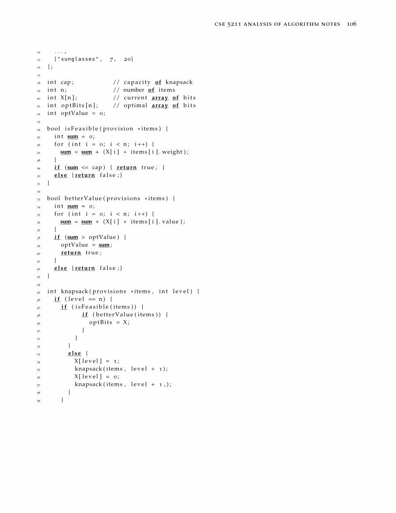
cse 5211 analysis of algorithm notes 106
14 . . . ,15 "sunglasses" , 7 , 20 16 ;17
18 i n t cap ; // c a p a c i t y of knapsack19 i n t n ; // number of i tems20 i n t X[ n ] ; // current array of b i t s21 i n t o p t B i t s [ n ] ; // optimal array of b i t s22 i n t optValue = 0 ;23
24 bool i s F e a s i b l e ( provis ion * items ) 25 i n t sum = 0 ;26 f o r ( i n t i = 0 ; i < n ; i ++) 27 sum = sum + (X[ i ] * i tems [ i ] . weight ) ;28 29 i f (sum <= cap ) return t rue ; 30 e lse return f a l s e ; 31 32
33 bool bet terValue ( provis ions * items ) 34 i n t sum = 0 ;35 f o r ( i n t i = 0 ; i < n ; i ++) 36 sum = sum + (X[ i ] * i tems [ i ] . value ) ;37 38 i f (sum > optValue ) 39 optValue = sum ;40 return t rue ;41 42 e lse return f a l s e ; 43 44
45 i n t knapsack ( provis ions * items , i n t l e v e l ) 46 i f ( l e v e l == n ) 47 i f ( i s F e a s i b l e ( i tems ) ) 48 i f ( be t terValue ( items ) ) 49 o p t B i t s = X ;50 51 52 53 e lse 54 X[ l e v e l ] = 1 ;55 knapsack ( items , l e v e l + 1 ) ;56 X[ l e v e l ] = 0 ;57 knapsack ( items , l e v e l + 1 , ) ;58 59
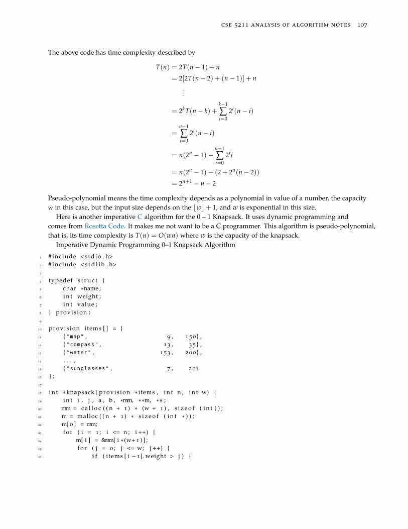
cse 5211 analysis of algorithm notes 107
The above code has time complexity described by
T(n) = 2T(n− 1) + n
= 2[2T(n− 2) + (n− 1)] + n...
= 2kT(n− k) +k−1
∑i=0
2i(n− i)
=n−1
∑i=0
2i(n− i)
= n(2n − 1)−n−1
∑i=0
2ii
= n(2n − 1)− (2 + 2n(n− 2))
= 2n+1 − n− 2
Pseudo-polynomial means the time complexity depends as a polynomial in value of a number, the capacityw in this case, but the input size depends on the bwc+ 1, and w is exponential in this size.
Here is another imperative C algorithm for the 0 – 1 Knapsack. It uses dynamic programming andcomes from Rosetta Code. It makes me not want to be a C programmer. This algorithm is pseudo-polynomial,that is, its time complexity is T(n) = O(wn) where w is the capacity of the knapsack.
Imperative Dynamic Programming 0–1 Knapsack Algorithm
1 # include < s t d i o . h>2 # include < s t d l i b . h>3
4 typedef s t r u c t 5 char *name ;6 i n t weight ;7 i n t value ;8 provis ion ;9
10 provis ion items [ ] = 11 "map" , 9 , 1 5 0 ,12 "compass" , 13 , 3 5 ,13 "water" , 153 , 2 0 0 ,14 . . . ,15 "sunglasses" , 7 , 20 16 ;17
18 i n t * knapsack ( provis ion * items , i n t n , i n t w) 19 i n t i , j , a , b , *mm, * *m, * s ;20 mm = c a l l o c ( ( n + 1 ) * (w + 1 ) , s i z e o f ( i n t ) ) ;21 m = malloc ( ( n + 1 ) * s i z e o f ( i n t * ) ) ;22 m[ 0 ] = mm;23 f o r ( i = 1 ; i <= n ; i ++) 24 m[ i ] = &mm[ i * (w+ 1 ) ] ;25 f o r ( j = 0 ; j <= w; j ++) 26 i f ( i tems [ i −1] . weight > j )
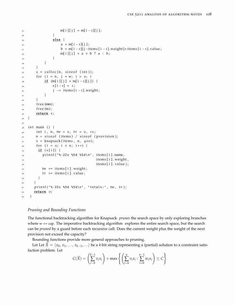
cse 5211 analysis of algorithm notes 108
27 m[ i ] [ j ] = m[ i −1][ j ] ;28 29 e lse 30 a = m[ i −1][ j ] ;31 b = m[ i −1][ j−i tems [ i −1] . weight ]+ items [ i −1] . value ;32 m[ i ] [ j ] = a > b ? a : b ;33 34 35 36 s = c a l l o c ( n , s i z e o f ( i n t ) ) ;37 f o r ( i = n , j = w; i > 0 ; i−−)38 i f (m[ i ] [ j ] > m[ i −1][ j ] ) 39 s [ i −1] = 1 ;40 j −= items [ i −1] . weight ;41 42 43 f r e e (mm) ;44 f r e e (m) ;45 return s ;46 47
48 i n t main ( ) 49 i n t i , n , tw = 0 , tv = 0 , * s ;50 n = s i z e o f ( i tems ) / s i z e o f ( provis ion ) ;51 s = knapsack ( items , n , 4 0 0 ) ;52 f o r ( i = 0 ; i < n ; i ++) 53 i f ( s [ i ] ) 54 p r i n t f ( "%-22s %5d %5d\n" , i tems [ i ] . name ,55 i tems [ i ] . weight ,56 i tems [ i ] . value ) ;57 tw += items [ i ] . weight ;58 tv += items [ i ] . value ;59 60 61 p r i n t f ( "%-22s %5d %5d\n" , "totals:" , tw , tv ) ;62 return 0 ;63
Pruning and Bounding Functions
The functional backtracking algorithm for Knapsack prunes the search space by only exploring brancheswhere w <= cap. The imperative backtracking algorithm explores the entire search space, but the searchcan be pruned by a guard before each recursive call: Does the current weight plus the weight of the nextprovision not exceed the capacity?
Bounding functions provide more general approaches to pruning.Let Let ~X = 〈x0, x1, . . . , xk−1, . . .〉 be a k-bit string representing a (partial) solution to a constraint satis-
faction problem. Let
C(~X) =
(k−1
∑i−0
vixi
)+ max
(n
∑i=k
vixi :n−1
∑i=0
wixi
)≤ C

cse 5211 analysis of algorithm notes 109
That is, C(~X) is the maximum value of feasible descendants (extensions) of ~X. It is the value of the currentlyselected provisions plus the largest value over the set of feasible extensions (descendants) of ~X.
In particular, if∣∣∣~X∣∣∣ = n, then ~X is a feasible solution, C(~X) is its value, but ~X may not be optimal. Also,
if∣∣∣~X∣∣∣ = 0, then C(~X) is the optimal value of the problem.
Bounding Function Properties
A bounding function B is any function defined on variable length bit strings such that
• If ~X is a feasible solution, the C(~X) = B(~X)
• For all partial feasible solutions, C(~X) ≤ B(~X)
If such a bounding function B() can be found, and if at any point of the computation B(~X) ≤ optValue
holds, then no extensions of ~X can lead to an optimal solution. And, searching descendants of ~X can bepruned.
Computing C(~X) is expensive when ~X has many descendants. The bounding function B() should bemuch easier to compute. And, we want B() be be a good approximation of C().
One trick that can lead to discovering a bounding function is to find a simpler, easier to solve, relatedproblems. A natural approximation to the 0–1 Knapsack problem is the Rational Knapsack problem (RK)
Recall, the greedy approach to the RK problem: Given a list of items, sort them in descending order intheir value-to-weight ratios. An item with value 10 and weight 3 is worth more than an item with value 10and weight 4. This sort only needs to be done once. Assume its time complexity is O(n lg n).
The greedy algorithm places items in the knapsack in order, one at a time as long as they fit. Somefraction of the last item might need to be used to fill, but not overfill, the knapsack. The time complexityis O(n). See the notes on Greedy algorithms.
Let ~X = 〈x0, x1, . . . , xk−1, . . .〉 be a string of k-bit strings representing a (partial) solution to a Knapsackproblem. Let R(k, C′) be the optimal solution to the Rational Knapsack problem with capacity C′, over allrational descendants of ~X, that is, 〈xk, xk+1, . . . , xn−1〉 where the values of xj ∈ Q, the set of rationals.
Define a bounding function by
B(~X) =k−1
∑i=0
xi pi + R
(k, C−
k−1
∑i=0
xiwi
)= CV + R(k, C− CW)
where CV is the current value and CW is the current weight.That is, B(~X) is the value selected provision from 0 to k− 1, plus the value that can be gained from the
remaining provisions using the remaining capacity and rational x’s. When all of the x’s are restricted to 0or 1, then C(X) = B(X). Also, since rational x’s yield more freedom (choices), C(X) ≤ B(X)
Here’s an example from (Stinson, 1987). Assume there are 5 items with weights
~W = 〈11, 12, 8, 7, 9〉
and values~V = 〈23, 24, 15, 13, 16〉
Pretend the knapsack’s capacity of C = 26. The weights and values are sorted by value-to-weight ratio:
〈23/11, 24/12, 15/8, 13/7, 16/9〉 ≈ 〈2.09, 2, 1.875, 1.857, 1.77〉
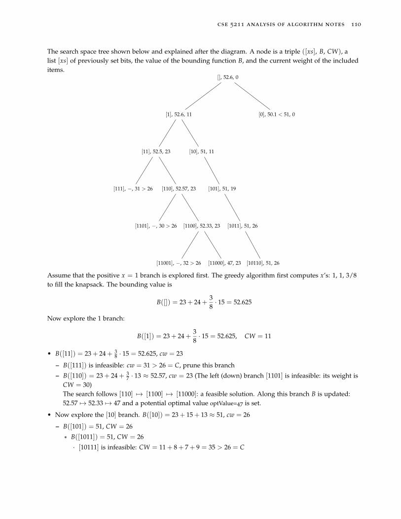
cse 5211 analysis of algorithm notes 110
The search space tree shown below and explained after the diagram. A node is a triple ([xs], B, CW), alist [xs] of previously set bits, the value of the bounding function B, and the current weight of the includeditems.
[], 52.6, 0
[1], 52.6, 11
[11], 52.5, 23
[111], −, 31 > 26 [110], 52.57, 23
[1101], −, 30 > 26 [1100], 52.33, 23
[11001], −, 32 > 26 [11000], 47, 23
[10], 51, 11
[101], 51, 19
[1011], 51, 26
[10110], 51, 26
[0], 50.1 < 51, 0
Assume that the positive x = 1 branch is explored first. The greedy algorithm first computes x’s: 1, 1, 3/8to fill the knapsack. The bounding value is
B([]) = 23 + 24 +38· 15 = 52.625
Now explore the 1 branch:
B([1]) = 23 + 24 +38· 15 = 52.625, CW = 11
• B([11]) = 23 + 24 + 38 · 15 = 52.625, cw = 23
– B([111]) is infeasible: cw = 31 > 26 = C, prune this branch
– B([110]) = 23 + 24 + 37 · 13 ≈ 52.57, cw = 23 (The left (down) branch [1101] is infeasible: its weight is
CW = 30)The search follows [110] 7→ [1100] 7→ [11000]: a feasible solution. Along this branch B is updated:52.57 7→ 52.33 7→ 47 and a potential optimal value optValue=47 is set.
• Now explore the [10] branch. B([10]) = 23 + 15 + 13 ≈ 51, cw = 26
– B([101]) = 51, CW = 26
* B([1011]) = 51, CW = 26
· [10111] is infeasible: CW = 11 + 8 + 7 + 9 = 35 > 26 = C

cse 5211 analysis of algorithm notes 111
· [10110] is feasible: B([10110]) = 51, CW = C, and a new, better, potential optimal valueoptValue=51 is set.
* B([100]) = (23) + 13 + 23 16 = 46.6 < 51, CW = 11. Since this value of B is less than the previously
computed optimal value 51 this branch can be pruned.
• When the [0] branch is explored, we find
B([0]) = 0 · 23 + 24 + 15 +67· 13 ≈ 50.14 < 51
Since this value of B is less than the previously computed potential optimal solution 51 its entire sub-tree can be pruned
The Traveling Salesman & Hamiltonian Circuit Problem
A Hamiltonian tour or circuit in an undirected graph G = (E, V) is a cycle that passes through each nodeexactly once. When the edges have non-negative weights, a traveling salesman want to find the shortesttour. Name the nodes 0 through n − 1. Since the tour is a cycle, the first node is arbitrary, and might aswell be 0. A tour is a permutation of 1, 2, . . . , (n− 1), so there are (n− 1)! possible tours. But, the graph isundirected, so a permutation [0, 1, 2, 3, 4, 5] is equivalent to [0, 5, 4, 3, 2, 1].
M =
a b c d
a ∞ 3 5 8b 3 ∞ 2 7c 5 2 ∞ 6d 8 7 6 ∞
An adjacency matrix can be reduced by subtracting the minimum in each row from itself and others in therow. Then, using this new matrix, subtract the minimum in each column from itself and the other values inthe column. Keep a running tab of the amount subtracted: Call the value V(M).
The resulting matrix has:
• All non-negative entries
• Every row and every column contains at least one 0.
a b c d
a ∞ 3 5 8b 3 ∞ 2 7c 5 2 ∞ 6d 8 7 6 ∞
7→
a b c d
a ∞ 0 2 5b 1 ∞ 0 6c 3 0 ∞ 4d 2 1 0 ∞
7→
a b c d
a ∞ 0 2 1b 0 ∞ 0 2c 2 0 ∞ 0d 1 1 0 ∞
With V(M) = (3 + 2 + 2 + 6) + (1 + 0 + 0 + 4) = 18.
V(M) is a lower bound on the cost of any Hamiltonian circuit. To see this, let
H = [0x1x2 · · · xn−1
be any tour: x1x2 · · · xn−1 is a permutation on the set 1, 2, . . . , (n− 1). The adjacency matrix entriesM[0, x1], M[x1, x2], . . . , M[xn−1, 0] cover all rows and columns. The sum of these entries is the cost of thetour H.
C(H) =n
∑i=1
M[xi−1, xi] x0 = xn = 0

cse 5211 analysis of algorithm notes 112
For each row i = 1, . . . , n, subtract M[xi−1, xi] from each entry in the row.
References
Stinson, D. R. (1987). An Introduction to the Design and Analysis of Algorithms. The Charles Babbage Re-search Center, P. O. Box 272, St. Norbert Postal Station, Winnipeg, Manitoba R3V 1L6, Canada, secondedition. [page 109]

cse 5211 analysis of algorithm notes 113
The Set Partition Problem
Can a set integers be partitioned into two non-empty subsets that have equal sums over
their values? This is an NP-complete problem. Given the two subsets, a linear algorithm adds theirvalues and tests for equality. A variant would ask for the absolute value of the difference in sums to be assmall as possible.
For example, the set S = 3, 1, 5, 7 can be partitioned as 3, 5 and 1, 7. While S = 3, 1, 5, 8 hasonly an unbalanced partition 3, 5 and 1, 8.
Stirling’s number of the second kind n2 counts the number of partitions of an n-element set into two
non-empty subsets. It can be shown that n2 = 2n−1 − 1. Therefore, except for small examples, it is infeasi-
ble to use brute-force and test every partition.A set of integers can be partitioned into two equal summing subsets only if the sum of all values is even.
And, the sum over either subset must be one-half of this total.A useful abstraction is to consider both summations to be over the entire set of integers. This is accom-
plished using a a bit vector〈b0, b1, b2, b3, . . .〉
where a particular bit bk is set to 1 or 0 depending on whether or not integer ik is or is not in a subset. Notall subsets need to be explored: Once a subset is infeasible so are all of its super-sets.
I could not get my Haskell implementation of Set Partition to work correctly. Here is an implementationfrom StackOverflow.
1 import Data . L i s t (minimumBy)2 minimumBy takes a comparison funct ion and a l i s t and3 re turns the l e a s t element of the l i s t by the comparison funct ion . The4 l i s t must be f i n i t e and non−empty . 5 import Data . Ord ( comparing )6 comparing takes a funct ion f and two values x and y . I t compares ( f x ) ( f y )7 Here i s a sample s e t of i n t e g e r s to p a r t i t i o n i n t o equal sums . 8 s e t = [ 9 0 , 13 , 153 , 50 , 15 , 68 , 27 , 39 , 23 , 52 , 11 , 32 , 24 , 48 , 4 , 73 , 18 , 30 , 42 , 43 , 22 , 7 ]9
10 p a r t i t i o n s generates a l l p a r t i t i o n s of a l i s t i n t o an ordered pai r11 of s u b l i s t s . Given a l i s t ( x : xs ) , compute the p a r t i t i o n s of the t a i l xs12 and c a l l the r e s u l t ps = ( ys , zs ) . Then place x a t the head of both ys and zs . 13 p a r t i t i o n s : : [ a ] −> [ ( [ a ] , [ a ] ) ]14 p a r t i t i o n s [ ] = [ ( [ ] , [ ] ) ]15 p a r t i t i o n s ( x : xs ) = l e t ps = p a r t i t i o n s xs16 in [ ( x : ys , zs ) | ( ys , zs ) <− ps ] ++ [ ( ys , x : zs ) |( ys , zs ) <− ps ]17 unbalance sums two l i s t and re turns the absolute value of the d i f f e r e n c e 18 unbalance : : Num a => ( [ a ] , [ a ] ) −> a19 unbalance ( ys , zs ) = abs (sum ys − sum zs )20 b a l a n c e P a r t i t i o n generates a l l two s u b l i s t p a r t i t i o n s of a l i s t . I t21 composes t h i s funct ion with unbalanced of non−negat ive22 values and compares them returning the minimum by doing t h i s . 23 b a l a n c e d P a r t i t i o n : : (Num a , Ord a ) => [ a ] −> ( [ a ] , [ a ] )24 b a l a n c e d P a r t i t i o n = minimumBy ( comparing unbalance ) . p a r t i t i o n s25
26 main = do print ( b a l a n c e d P a r t i t i o n s e t )
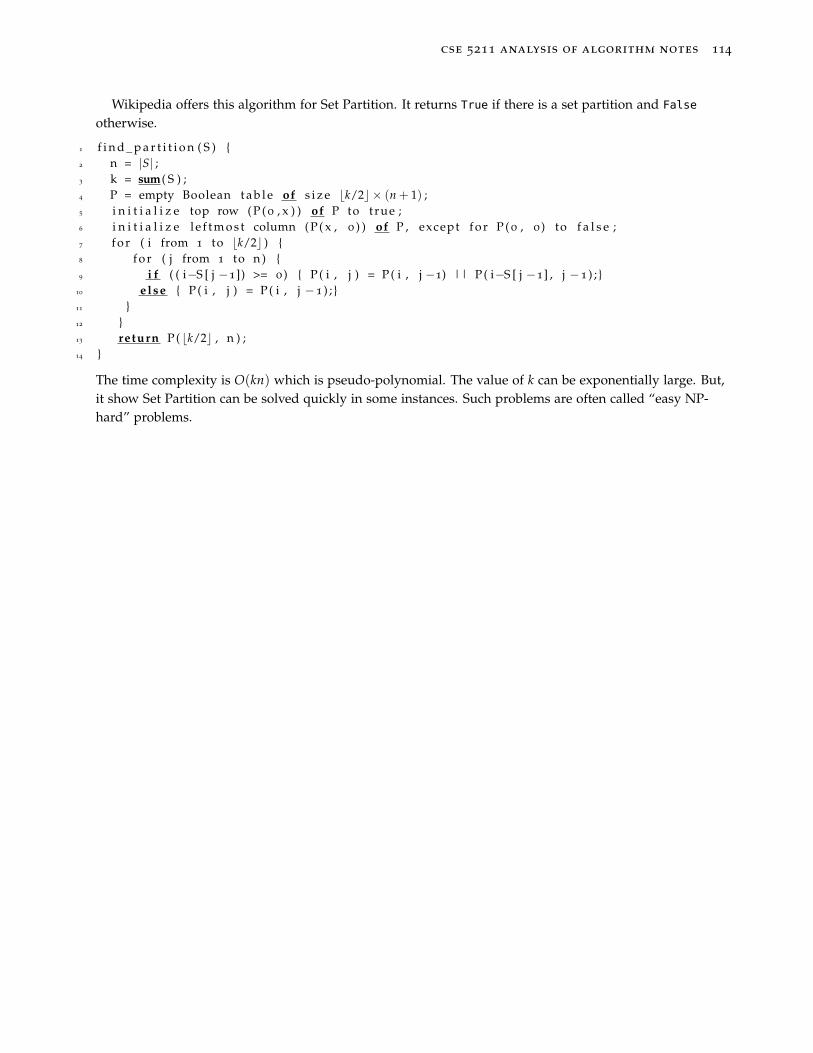
cse 5211 analysis of algorithm notes 114
Wikipedia offers this algorithm for Set Partition. It returns True if there is a set partition and False
otherwise.
1 f i n d _ p a r t i t i o n ( S ) 2 n = |S| ;3 k = sum( S ) ;4 P = empty Boolean t a b l e of s i z e bk/2c × (n + 1) ;5 i n i t i a l i z e top row ( P ( 0 , x ) ) of P to true ;6 i n i t i a l i z e l e f t m o s t column ( P ( x , 0 ) ) of P , except f o r P ( 0 , 0 ) to f a l s e ;7 f o r ( i from 1 to bk/2c ) 8 f o r ( j from 1 to n ) 9 i f ( ( i−S [ j −1]) >= 0 ) P ( i , j ) = P ( i , j −1) || P ( i−S [ j −1] , j −1 ) ;
10 e lse P ( i , j ) = P ( i , j −1 ) ; 11 12 13 return P ( bk/2c , n ) ;14
The time complexity is O(kn) which is pseudo-polynomial. The value of k can be exponentially large. But,it show Set Partition can be solved quickly in some instances. Such problems are often called “easy NP-hard” problems.

cse 5211 analysis of algorithm notes 115
Complexity
Problems can be classified by at least two types: Decision and Function Problems.
• A decision problem is a question with a “yes” (True) or “no” (False) answer. For instance, are values inlist ~X ascending?
• A function problem requires a solution to the problem. Sort values in list ~X into ascending order.
Function problems are typically harder than decision problems.
Good decision problems come from consistent theories. Example axiomatic theories (models)include: Arithmetic, Boolean (propositional) logic, and first-order (predicate) logic.
• A theory or model is consistent if it does not contain a contradiction: Only one of p or ¬p can have aproof.
• A model is complete when at least one of p or ¬p has a proof.
• A problem within a model is decidable if there is an algorithm that always answers the problem correctly.
There are some unfortunate results.
Gödel’s First Incompleteness Theorem.
“Every consistent formal proof system about a sufficiently rich arithmetic is incomplete.”
The theorem says there are statements about the arithmetic we learn as children that are True but have noproof.
Gödel’s Second Incompleteness Theorem
“If a formal proof system about a sufficiently rich arithmetic is consistent, there is no proof that it is consistent.”
Gödel’s second theorem says you cannot prove a consistent arithmetic is consistent.
Complexity can be defined by a hierarchy of problem classes. Some relationships among theseclasses are unknown. Here is an image from (Papadimitriou, 1994) (created by Sebastian Sardina) thatshows the relationship among several complexity classes under common assumptions that have not beenfully proven. Computational complexity is complex.

cse 5211 analysis of algorithm notes 116
LOGTime
LOGSpace
P NP
NPC
co-N
P
PSPACE
EXPTIME
EXPSPACE
...ELEMENTARY
...2EXPTIME
R
• The class P: Problems that can be correctly solved in polynomial time using a deterministic Turing ma-chine. Exercise: List some problems that belong to P.
• The class NP: Problems that can be solved in polynomial time using a non-deterministic Turing ma-chine.
Problem in class NP are characterized by the idea that answers can be checked for correctness quickly,that is, in polynomial time on a deterministic Turing machine.
Exercise: List some problems that belong to NP, but are not known to be in P.
Every problem in P is in NP (P ⊆ NP). If a problem can be solved in polynomial time, it can be checked inpolynomial time. Deterministic time is a subset of non-deterministic time.
The central question in complexity theory is:
Does P ?= N P.
Most people who understand the question believe, I believe, the answer is “no,” but there is no proofone way or another, so shrug your shoulders.
There are problems in NP that are not known to be in P:
• Is a Boolean expression satisfiable? There are 2n truth assignments when the expression has n variables.To find satisfying truth assignment may require search over this large space.
However, checking that a truth assignment satisfies an expression is straightforward.
The complementary problem: Is a Boolean expression unsatisfiable seem even harder: Every truth assign-ment must results in a False value. Unsatisfiable is in co-NP.

cse 5211 analysis of algorithm notes 117
• Given a set of integers is there partition that has equal sums? There are 2n−1 − 1 ways to partition ann-element set into two subsets.
But, given a proposed two-set partition, it is easy to check that their sums are identical.
• Does a subset of graph vertices cover the graph? That is, each edge is incident on some vertex in thesubset. Again, lots of subsets. Easy to check that one is a vertex cover.
• Does a graph have a Hamiltonian circuit (tour)? Again, lots of paths. Easy to check that one is a Hamil-tonian tour.
Reduction is a problem solving strategy. Suppose there is an algorithm A that solves instancesof problem p. Given a new problem q suppose there is an algorithm R that reduces instances of q intoinstances of problem p. Then an instance of problem q can be solved by applying R to to get an instance ofp and apply A to it to solve the original instance.
The reduction R is always assumed to be deterministic and polynomial in time.
Q R7→ pA7→ True, False
There are several conclusions that can be drawn when a reduction R exists.
• If p ∈ P, then q ∈ P.
• If p is decidable, then q is decidable.
• If q ∈ NP, then p ∈ NP.
• If q is undecidable, then p is undecidable (algorithm A does not exist).
The concept of reductions leads to complete and hard complexity classes.
Complete and Hard Problems
Complete problems are the hardest in a problem class; hard problems may not even be-long to the class.
Let K be a complexity class.
• A problem p ∈ K is K-complete if every problem q in K can be reduced to p using some deterministic,polynomial time algorithm.
• A problem p is K-hard if every problem q in K can be reduced p.
For the For the class NP of non-deterministic polynomial time problems Euler’s diagram of the relation-ships between NP, NP-complete, and NP-hard depends on the answer to the question
P ?= NP
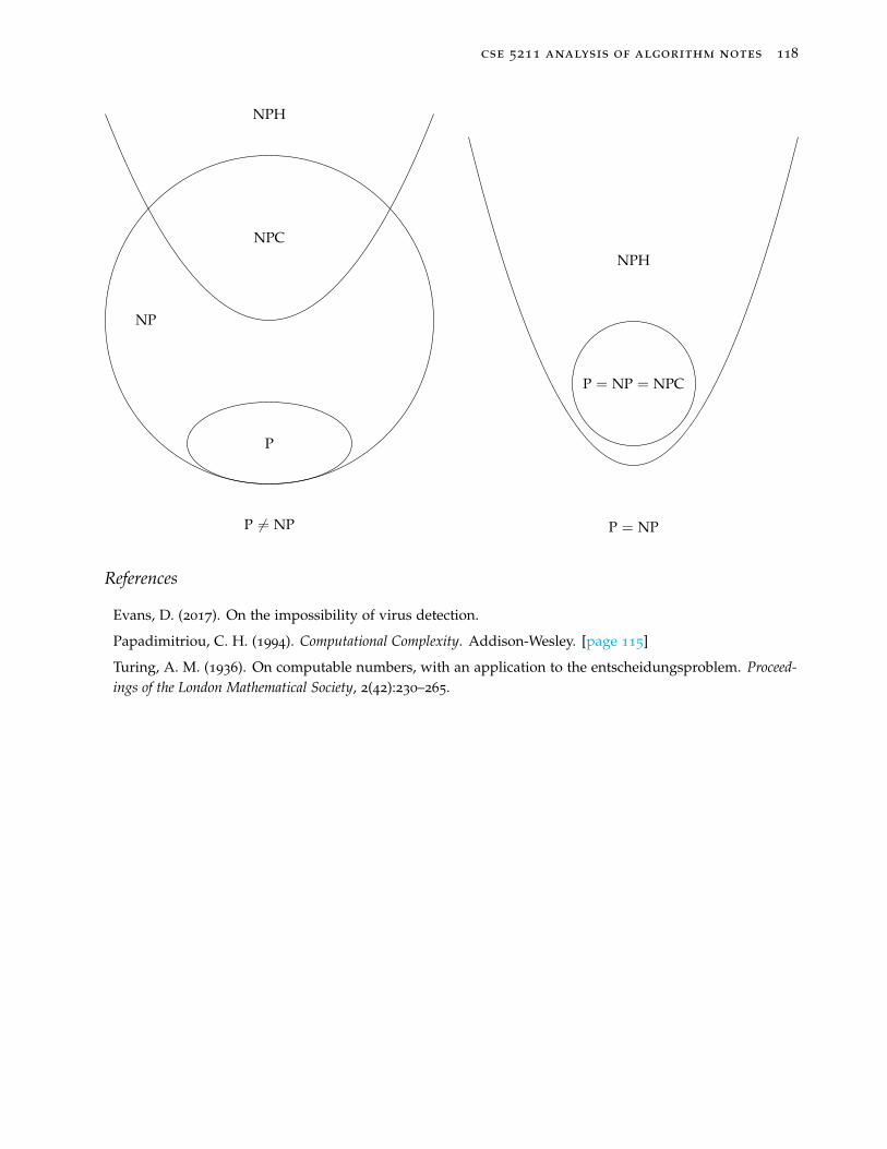
cse 5211 analysis of algorithm notes 118
P
NP
NPC
NPH
P 6= NP
P = NP = NPC
NPH
P = NP
References
Evans, D. (2017). On the impossibility of virus detection.
Papadimitriou, C. H. (1994). Computational Complexity. Addison-Wesley. [page 115]
Turing, A. M. (1936). On computable numbers, with an application to the entscheidungsproblem. Proceed-ings of the London Mathematical Society, 2(42):230–265.
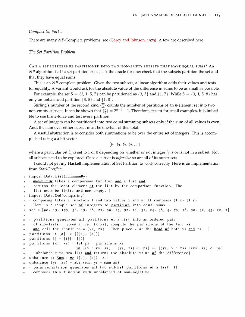
cse 5211 analysis of algorithm notes 119
Complexity, Part 2
There are many NP-Complete problems, see (Garey and Johnson, 1979). A few are described here.
The Set Partition Problem
Can a set integers be partitioned into two non-empty subsets that have equal sums? AnNP algorithm is: If a set partition exists, ask the oracle for one; check that the subsets partition the set andthat they have equal sums.
This is an NP-complete problem. Given the two subsets, a linear algorithm adds their values and testsfor equality. A variant would ask for the absolute value of the difference in sums to be as small as possible.
For example, the set S = 3, 1, 5, 7 can be partitioned as 3, 5 and 1, 7. While S = 3, 1, 5, 8 hasonly an unbalanced partition 3, 5 and 1, 8.
Stirling’s number of the second kind n2 counts the number of partitions of an n-element set into two
non-empty subsets. It can be shown that n2 = 2n−1 − 1. Therefore, except for small examples, it is infeasi-
ble to use brute-force and test every partition.A set of integers can be partitioned into two equal summing subsets only if the sum of all values is even.
And, the sum over either subset must be one-half of this total.A useful abstraction is to consider both summations to be over the entire set of integers. This is accom-
plished using a a bit vector〈b0, b1, b2, b3, . . .〉
where a particular bit bk is set to 1 or 0 depending on whether or not integer ik is or is not in a subset. Notall subsets need to be explored: Once a subset is infeasible so are all of its super-sets.
I could not get my Haskell implementation of Set Partition to work correctly. Here is an implementationfrom StackOverflow.
1 import Data . L i s t (minimumBy)2 minimumBy takes a comparison funct ion and a l i s t and3 re turns the l e a s t element of the l i s t by the comparison funct ion . The4 l i s t must be f i n i t e and non−empty . 5 import Data . Ord ( comparing )6 comparing takes a funct ion f and two values x and y . I t compares ( f x ) ( f y )7 Here i s a sample s e t of i n t e g e r s to p a r t i t i o n i n t o equal sums . 8 s e t = [ 9 0 , 13 , 153 , 50 , 15 , 68 , 27 , 39 , 23 , 52 , 11 , 32 , 24 , 48 , 4 , 73 , 18 , 30 , 42 , 43 , 22 , 7 ]9
10 p a r t i t i o n s generates a l l p a r t i t i o n s of a l i s t i n t o an ordered pai r11 of sub− l i s t s . Given a l i s t ( x : xs ) , compute the p a r t i t i o n s of the t a i l xs12 and c a l l the r e s u l t ps = ( ys , zs ) . Then place x a t the head of both ys and zs . 13 p a r t i t i o n s : : [ a ] −> [ ( [ a ] , [ a ] ) ]14 p a r t i t i o n s [ ] = [ ( [ ] , [ ] ) ]15 p a r t i t i o n s ( x : xs ) = l e t ps = p a r t i t i o n s xs16 in [ ( x : ys , zs ) | ( ys , zs ) <− ps ] ++ [ ( ys , x : zs ) |( ys , zs ) <− ps ]17 unbalance sums two l i s t and re turns the absolute value of the d i f f e r e n c e 18 unbalance : : Num a => ( [ a ] , [ a ] ) −> a19 unbalance ( ys , zs ) = abs (sum ys − sum zs )20 b a l a n c e P a r t i t i o n generates a l l two s u b l i s t p a r t i t i o n s of a l i s t . I t21 composes t h i s funct ion with unbalanced of non−negat ive
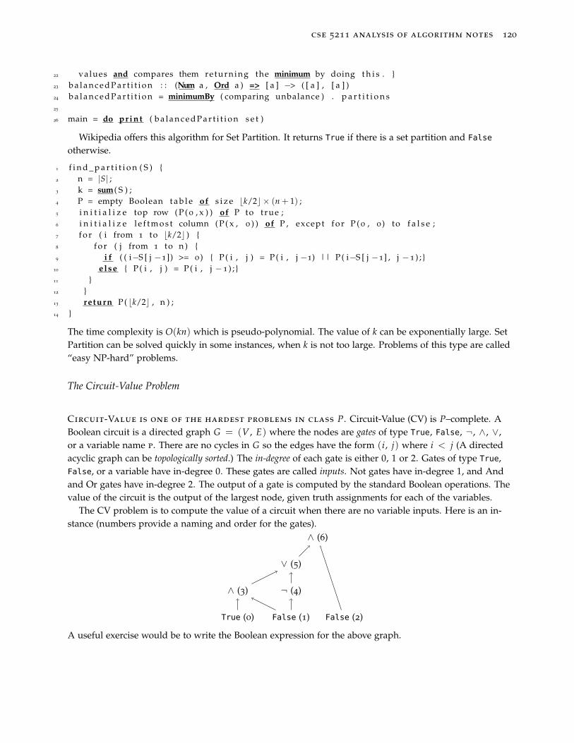
cse 5211 analysis of algorithm notes 120
22 values and compares them returning the minimum by doing t h i s . 23 b a l a n c e d P a r t i t i o n : : (Num a , Ord a ) => [ a ] −> ( [ a ] , [ a ] )24 b a l a n c e d P a r t i t i o n = minimumBy ( comparing unbalance ) . p a r t i t i o n s25
26 main = do print ( b a l a n c e d P a r t i t i o n s e t )
Wikipedia offers this algorithm for Set Partition. It returns True if there is a set partition and False
otherwise.
1 f i n d _ p a r t i t i o n ( S ) 2 n = |S| ;3 k = sum( S ) ;4 P = empty Boolean t a b l e of s i z e bk/2c × (n + 1) ;5 i n i t i a l i z e top row ( P ( 0 , x ) ) of P to true ;6 i n i t i a l i z e l e f t m o s t column ( P ( x , 0 ) ) of P , except f o r P ( 0 , 0 ) to f a l s e ;7 f o r ( i from 1 to bk/2c ) 8 f o r ( j from 1 to n ) 9 i f ( ( i−S [ j −1]) >= 0 ) P ( i , j ) = P ( i , j −1) || P ( i−S [ j −1] , j −1 ) ;
10 e lse P ( i , j ) = P ( i , j −1 ) ; 11 12 13 return P ( bk/2c , n ) ;14
The time complexity is O(kn) which is pseudo-polynomial. The value of k can be exponentially large. SetPartition can be solved quickly in some instances, when k is not too large. Problems of this type are called“easy NP-hard” problems.
The Circuit-Value Problem
Circuit-Value is one of the hardest problems in class P. Circuit-Value (CV) is P–complete. ABoolean circuit is a directed graph G = (V , E) where the nodes are gates of type True, False, ¬, ∧, ∨,or a variable name p. There are no cycles in G so the edges have the form (i, j) where i < j (A directedacyclic graph can be topologically sorted.) The in-degree of each gate is either 0, 1 or 2. Gates of type True,False, or a variable have in-degree 0. These gates are called inputs. Not gates have in-degree 1, and Andand Or gates have in-degree 2. The output of a gate is computed by the standard Boolean operations. Thevalue of the circuit is the output of the largest node, given truth assignments for each of the variables.
The CV problem is to compute the value of a circuit when there are no variable inputs. Here is an in-stance (numbers provide a naming and order for the gates).
True (0)
∧ (3)
∨ (5)
∧ (6)
False (1)
¬ (4)
False (2)
A useful exercise would be to write the Boolean expression for the above graph.

cse 5211 analysis of algorithm notes 121
To show CV is P–complete two things must be shown:
1. CV∈ P. Describe a polynomial time, deterministic algorithm that computes the value of a circuit.
For the example circuit, evaluate it by traversing it in topological order:
(0, 3), (1, 3), (1, 4), (3, 5), (4, 5), (5, 6), (2, 6)
2. If L ∈ P, there is a polynomial time deterministic reduction R of instances in L to instances in CV.
Given any input x, R(x) must be a variable-free circuit such that x ∈ L if and only if R(x) is True. Theconstruction of R is complex and beyond my ability to summarize. See (Papadimitriou, 1994) for details.The fact that such a reduction R exist is amazing.
Cook (Cook, 1971) and Levin (Levin, 1973) demonstrated the existence of N P–Complete
problems. Karp (Karp, 1972) showed how to reduce many problems to known N P–complete problems.The book by Garey and Johnson (Garey and Johnson, 1979) documents innumerable hard problems. Beforeyou undertake the task of finding a problem solution, know complexity of the problem.
Recall, colloquially a problem L is in N P if each instance x has a short certificate that can be checked andreturns True if x ∈ L and False otherwise.
Satisfiability (SAT) is the classic N P–complete example: Given a Boolean expression φ (in conjunctivenormal form) is φ satisfiable? That is, is there a truth assignment for the variables in φ that makes φ True.
Conjunctive normal form (CNF) means: φ is the And of Or phrases, called clauses. All expressions canbe represented in CNF. The basics of the reduction is to replace conditionals p ⇒ q with ¬pro p p ∨ q.Distribute Nots using De Morgan’s laws and eliminate double negations. And finally, distribute Ors acrossAnds. Unfortunately the conversion (reduction) to CNF can produce expressions of size 2n where n is thenumber of propositions in the original expression. But, CNF captures the difficulty of the problem. And,the test for satisfiability reasonable: For the given truth assignment, every clause must be True.
SAT an example of a P–hard problem. Any (simple) problem in P can be reduces to an instance of SAT.But SAT is not known to be in P, most likely SAT 6= P, but know one knows for sure (at this point in time).
Just as a Circuit-Value represents Boolean expressions with fixed truth assignments, Circuit-SAT rep-resents Boolean expressions with variable input. That a reduction from SAT to Circuit-SAT exists may beclear. Explaining and understanding the details is best done off-line.
It is interesting that 2–SAT has a polynomial time algorithm. In an instance of 2–SAT each clause hastwo literals. On the other hand, 3–SAT is N P–complete.
The complement of N P problems is an interesting class. The class co–N P consist of problemswhose complement are in N P.
Validity (VAL) is stronger than satisfiable: All truth assignments make φ True. A Boolean expression isvalid if and only if its negation is unsatisfiable (always False). Unsatisfiable (UNSAT) is the complement ofSAT.Definition. A decision problem L is in co-C if its negation is in C.
For instance, the problem “are the values in list ~X in ascending order?” is in P. It’s complement, “arethe values in list ~X not in ascending order?” is also in P.
It is not too hard to understand that co-P = P. If a decision problem can be decided “yes” or “no” inpolynomial time, then so can its complement Think of feeding an problem instance into a machine (pro-gram). If the machine says “yes” the complement machine says “no” and vice versa.
cse 5211 analysis of algorithm notes 122
On the other hand, it is not known where or not co-N P = N P, and most suspect, I suspect, would sayno, they are not equal. Consider: Does no truth assignment satisfy an expression? Is there no Hamiltoniantour in a graph? Is there no non-empty subset of a given set integers that sum to 0? In each case, it seemsevery possible solution must be tested.
Problems that are N P–hard are interesting too. An N P–hard problem H is one where everyL ∈ N P problem can be reduced to H. The halting problem is N P–hard. Halting is undecidable. There is noknown certificate the demonstrates a program P will halt on input x. But, every problem in P or N P canbe reduced to an instance of halting, not that that should be done.
References
Cook, S. A. (1971). The complexity of theorem-proving procedures. In Proceedings of the Third Annual ACMSymposium on Theory of Computing, STOC ’71, pages 151–158, New York, NY, USA. ACM. [page 121]
Garey, M. R. and Johnson, D. S. (1979). Computers and Intractability: A Guide to the Theory of Intractability.W. H. Freeman. [page 119], [page 121]
Karp, R. M. (1972). Reducibility among combinatorial problems. In Thatcher, J. W. and Miller, R. E.,editors, Complexity of Computer Computations, pages 85–103. Plenum Press, New York. [page 121]
Levin, L. A. (1973). Universal sorting problems. Problems of Information Transmission, 9:265–266. [page 121]
Papadimitriou, C. H. (1994). Computational Complexity. Addison-Wesley. [page 121]
cse 5211 analysis of algorithm notes 123
Computability
The theory of computation focuses on several topics. One is the complexity of problems: If aproblem can be solved, at what costs? Another topic is computational models: What are the mechanismsfor expressing and implementing solutions?
Turing machine, λ-calculus, recursive functions, and other computational models have been proposed.All sufficiently strong models have been shown to be equivalent. They solve the same class of problems.There are many ways to define a Turing machine. Here is Papadimitriou’s (Papadimitriou, 1994) definition.A deterministic Turing machine is a 4-tuple M = (K, Σ, δ, s) where:
1. K is a finite set of states
2. s ∈ K is the initial (start) state
3. Σ is an alphabet (a finite set of symbols). Σ contains two special symbols: t and ., called blank and first,respectively.
4. δ is a transition function. It maps a (state, character) pair to a triple (next state, character, direction).
δ : (K, Σ) → (K ∪ h, y, n , Σ, ←, →, —)
A non-deterministic Turing machine is the same, except δ is a choice relation mapping a (state, character) tosubsets of (state, character, direction) triples.
The Universal Turing Machine
Turing showed (Turing, 1936) an important aspect of his machine: There is a single universal Turing ma-chine U that can simulate any other Turing machine. The input to the U is a (machine description, input) pair(M, x). The universal machine U computes M(x), that is U(M, x) = M(x).
The existence of a universal machine leads to undecidable problems, the most famous of which is theHaltling Problem.
Decision Problem: Given a Turing machine M and its input x, does M halt on x?There is no algorithm that decides the halting problem. It may be possible to decide if a particular ma-
chine M halts on a particular input x, but there is no algorithm that answers the halting problem for everyinstance of M and x.
Define the halting language H is the set of all (machine, input) pairs such that M halts on x.
H = (M, x) : M(x) 6= ( means does not halt)
There is no Turing machine that decides whether or not (M, x) ∈ H for all pairs (M, x). The proof is bycontradiction.
Consider the thought experiment: Execute the diagonalMachine pseudo-code below. It assumes haltingcan be determined somehow. The program accepts the encoding of a machine M as input. It runs M onM, and loops forever if M(M) halts. If M(M) does not halt, then the diagonal machine halts. The main
routine runs diagonalMachine on itself. The term diagonalization comes from Cantor’s proof that the realnumbers are uncountable.
1 diagonalMachine ( machine M)

cse 5211 analysis of algorithm notes 124
2 i f (M(M) h a l t s ) then ; 3 e lse h a l t ;4 5
6 main diagonalMachine ( diagonalMachine ) ;
Now consider the logic:
• If diagonalMachine(diagonalMachine) halts, then diagonalMachine(diagonalMachine) loops forever, that is,diagonalMachine(diagonalMachine) does not halt.
• On the other hand, if diagonalMachine(diagonalMachine) does not halt, then diagonalMachine(diagonalMachine)
halts.
There is a contradiction in both cases. Therefore, the assumption that halting can be determined is wrong.There is no algorithm that correctly solves the halting decision problem:
“For all Turing machines M and for all inputs x, does M halt on x?”
The traditional proof that the halting problem is undecidable goes something like this:
Proof that the Halting Problem is undecidable. Pretend there is a Turing machine MH that de-cides the halting problem.
MH
(M, x) M(x) 6= (M halts on x)
M(x) = (M does not halt on x)
Use MH to construct a Turing machine D that accepts the encoding of a Turing machine M and runs MH
on (M, M). The behavior of D is this:
1. D does not halt if M halts on M.
If (M(M) 6=), then D(M) = (D(M) produces no output).
2. D halts if M does not halt on M.
If (M(M) =), then D(M) 6= (D(M) reports M does not halt on M).
DM
M does not halt on M
Now consider D(D).
DD
D does not halt on D
1. D does not halt (on input D) if D halts on D
If (D(D) 6=), then D(D) =.
2. D halts (on input D), if D does not halt on D
cse 5211 analysis of algorithm notes 125
If (D(D) =), then D(D) 6=
This contradiction implies that the halting machine MH cannot exist.
The Virus Problem
Evans presents a nice description of the virus problem (VP), see On the Impossibility of Virus Detection(Evans, 2017).
A virus is a computer program that when executed will copy its own code into another program. A virusdetection algorithm would act like this:
• Input: A description of a program P and its input x.
• Output: If P(x) behaves like a virus (running it infects other files) output True. Otherwise, outputFalse.
Assume there a program, virusDetect, that decides the Virus Problem (VP).
1 Boolean vi rusDetec t ( program P , input x ) 2 i f ( P ( x ) behaves l i k e a vi rus ) then t rue ;3 e lse f a l s e ;4
Here is the diagonalization argument that virus detection is undecidable. Assume there isa virus V. Mimic the argument above about the halting problem. That is, write a program, call it D(P) ifyou like, that uses virusDetect, to create a contradiction.
The idea behind D is to use virusDetect to check if the input P is a virus, and then do the opposite. Thatis,
• If P is a virus, D(P) simply halts without executing a virus.
• If P is not a virus, D(P) executes virus V.
1 D( program P ) 2 i f ( v i rusDetec t ( P , P ) ) then h a l t ;3 e lse V;4
Now consider the execution of D on itself.
• If D(D) acts like a virus, (That is, if VirusDetect(D, D))=true), then D(D) halts, That is, D(D) never exe-cutes a virus V.
(If D(D) is a virus, then D(D) does not act like a virus.)
• On the other hand, if D(D) is a not a virus, then D(D) executes virus V acting like a virus.
(If D(D) is not a virus, then D(D) acts like a virus.)
There are a contradictions in both cases.
Reduction of HP to VPSpend a few minutes going over Evans’ note On the Impossibility of Virus Detection.Another way to show the virus problem is undecidable is to show HP reduces to VP. That is, if VP were
decidable, then HP would be decidable. And, since HP is undecidable, VP must be also.
cse 5211 analysis of algorithm notes 126
The main idea is to construct a program makeVirus that first executes any input program P, and thenserially, if P halts, executes virus V.
1 makeVirus ( program P ) P ; V;
Argue that program halt below decides the halting problem. Use this to conclude there cannot be a virusdetection decider.
1 h a l t ( program P ) 2 i f ( v i rusDetec t ( makeVirus , P ) ) then t rue ;3 e lse f a l s e ;4
• If P halts, makeVirus will execute virus V and virusDetect(makeVirus,\ P) will return True.
• On the other hand, if P does not halt, then makeVirus will never execute V and virusDetect(makeVirus, P)
will return False.
In both cases the halting problem is correctly decided. Since this is not possible, there cannot be a virus de-tection program. There are a few wrinkles to iron out to fully nail down the argument. See (Evans, 2017).
References
Evans, D. (2017). On the impossibility of virus detection. [page 125], [page 126]
Papadimitriou, C. H. (1994). Computational Complexity. Addison-Wesley. [page 123]
Turing, A. M. (1936). On computable numbers, with an application to the Entscheidungsproblem. Proceed-ings of the London Mathematical Society, 2(42):230–265. [page 123]

cse 5211 analysis of algorithm notes 127
Search in Text
Searching for a pattern in a string is a classic problem. Search algorithm are built on fundamental con-cepts.
• A finite alphabet, Σ of characters, e.g., Σ could be Unicode.
• An equality relation defined on characters in Σ.
• Strings over Σ, defined recursively:
– The empty string λ, with no characters, is a string.
– Each member a ∈ Σ is a string.
– If s and t are strings, then their concatenation st is a string.
Σ∗ is the set of all strings over Σ. The set of all non-empty strings is denoted Σ+. N.
• A language L L is a subset of Σ∗.
• A word w ∈ L is a member of L.
• A language L is decidable if there is an algorithm that correctly decides the question: Is s ∈ L? for allstrings s ∈ Σ∗.
Decision Problem: Given a pattern (word) p and text (a string) t, does p occur in t?Function Problem: Given a pattern p and text t, find all places where p occur in t, if at all.
Imagine applications wherepattern matching could beuseful.
Imagine applications wherepattern matching could beuseful.Pattern matching
We will study several algorithms for pattern match. We are interested in their implementation and theirtime and space complexities. Some auxiliary functions will be introduced as needed. Here is the outline forthe notes.
127 〈Pattern match 127〉≡〈Brute-force pattern matching with left-to-right scan 128〉〈Morris-Pratt pattern matching ??〉
% 〈Knuth-Morris-Pratt pattern matching ??〉% 〈Brute-force pattern matching with right-to-left scan ??〉% 〈Boyer-Moore pattern matching ??〉% 〈Auxiliary functions 131a〉〈Test the pattern matching algorithms ??〉

cse 5211 analysis of algorithm notes 128
Let’s start with the brute-force approach: It solves the problem and leads to optimization ideas.
Brute force pattern matching
The brute-force approach is simple. As long as the pattern has not been found continue searching the textuntil the last legal position in the text has past.
Initial configuration
text a b a a b a a a b a a b a
pattern a b b a
Legal configuration last legal position
↓text a b a a b a a a b a a b a
pattern a b b a
Illegal configuration
text a b a a b a a a b a a b a
pattern a b b a
Here’s an description of the algorithm written in Haskell. Call it bfpm for short, althougth its name couldbe shorter or longer. The ideas are:
• An empty pattern matches any text.
• No pattern match empty text, except the empty pattern by the previous rule.
• The pattern matches the text if the head does and the tails of both match.
• Otherwise, the pattern matches the text if the pattern matches the tail of the text.
128 〈Brute-force pattern matching with left-to-right scan 128〉≡bfpm :: String -> String -> Bool
bfpm [] _ = True
bfpm _ [] = False
bfpm pattern text
| head pattern == head text = bfpm (tail pattern) (tail text)
| otherwise = bfpm pattern (tail text)
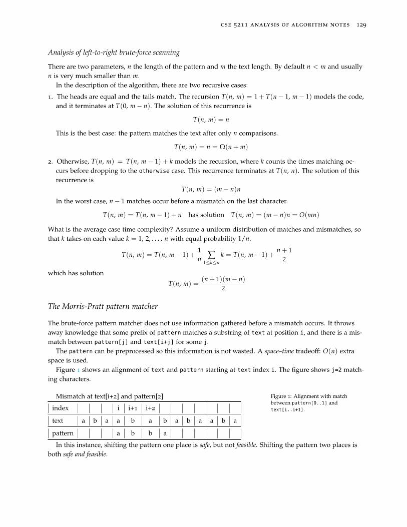
cse 5211 analysis of algorithm notes 129
Analysis of left-to-right brute-force scanning
There are two parameters, n the length of the pattern and m the text length. By default n < m and usuallyn is very much smaller than m.
In the description of the algorithm, there are two recursive cases:
1. The heads are equal and the tails match. The recursion T(n, m) = 1 + T(n− 1, m− 1) models the code,and it terminates at T(0, m− n). The solution of this recurrence is
T(n, m) = n
This is the best case: the pattern matches the text after only n comparisons.
T(n, m) = n = Ω(n + m)
2. Otherwise, T(n, m) = T(n, m − 1) + k models the recursion, where k counts the times matching oc-curs before dropping to the otherwise case. This recurrence terminates at T(n, n). The solution of thisrecurrence is
T(n, m) = (m− n)n
In the worst case, n− 1 matches occur before a mismatch on the last character.
T(n, m) = T(n, m− 1) + n has solution T(n, m) = (m− n)n = O(mn)
What is the average case time complexity? Assume a uniform distribution of matches and mismatches, sothat k takes on each value k = 1, 2, . . . , n with equal probability 1/n.
T(n, m) = T(n, m− 1) +1n ∑
1≤k≤nk = T(n, m− 1) +
n + 12
which has solution
T(n, m) =(n + 1)(m− n)
2
The Morris-Pratt pattern matcher
The brute-force pattern matcher does not use information gathered before a mismatch occurs. It throwsaway knowledge that some prefix of pattern matches a substring of text at position i, and there is a mis-match between pattern[j] and text[i+j] for some j.
The pattern can be preprocessed so this information is not wasted. A space–time tradeoff: O(n) extraspace is used.
Figure 1 shows an alignment of text and pattern starting at text index i. The figure shows j=2 match-ing characters.
Mismatch at text[i+2] and pattern[2]
index i i+1 i+2
text a b a a b a b a b a a b a
pattern a b b a
Figure 1: Alignment with matchbetween pattern[0..1] andtext[i..i+1].
In this instance, shifting the pattern one place is safe, but not feasible. Shifting the pattern two places isboth safe and feasible.
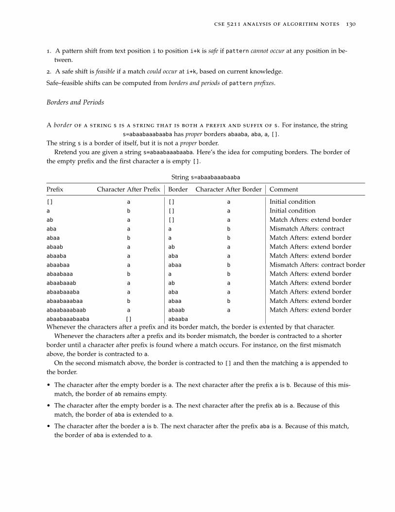
cse 5211 analysis of algorithm notes 130
1. A pattern shift from text position i to position i+k is safe if pattern cannot occur at any position in be-tween.
2. A safe shift is feasible if a match could occur at i+k, based on current knowledge.
Safe–feasible shifts can be computed from borders and periods of pattern prefixes.
Borders and Periods
A border of a string s is a string that is both a prefix and suffix of s. For instance, the strings=abaabaaabaaba has proper borders abaaba, aba, a, [].
The string s is a border of itself, but it is not a proper border.Rretend you are given a string s=abaabaaabaaba. Here’s the idea for computing borders. The border of
the empty prefix and the first character a is empty [].
String s=abaabaaabaaba
Prefix Character After Prefix Border Character After Border Comment
[] a [] a Initial conditiona b [] a Initial conditionab a [] a Match Afters: extend borderaba a a b Mismatch Afters: contractabaa b a b Match Afters: extend borderabaab a ab a Match Afters: extend borderabaaba a aba a Match Afters: extend borderabaabaa a abaa b Mismatch Afters: contract borderabaabaaa b a b Match Afters: extend borderabaabaaab a ab a Match Afters: extend borderabaabaaaba a aba a Match Afters: extend borderabaabaaabaa b abaa b Match Afters: extend borderabaabaaabaab a abaab a Match Afters: extend borderabaabaaabaaba [] abaaba
Whenever the characters after a prefix and its border match, the border is extented by that character.Whenever the characters after a prefix and its border mismatch, the border is contracted to a shorter
border until a character after prefix is found where a match occurs. For instance, on the first mismatchabove, the border is contracted to a.
On the second mismatch above, the border is contracted to [] and then the matching a is appended tothe border.
• The character after the empty border is a. The next character after the prefix a is b. Because of this mis-match, the border of ab remains empty.
• The character after the empty border is a. The next character after the prefix ab is a. Because of thismatch, the border of aba is extended to a.
• The character after the border a is b. The next character after the prefix aba is a. Because of this match,the border of aba is extended to a.
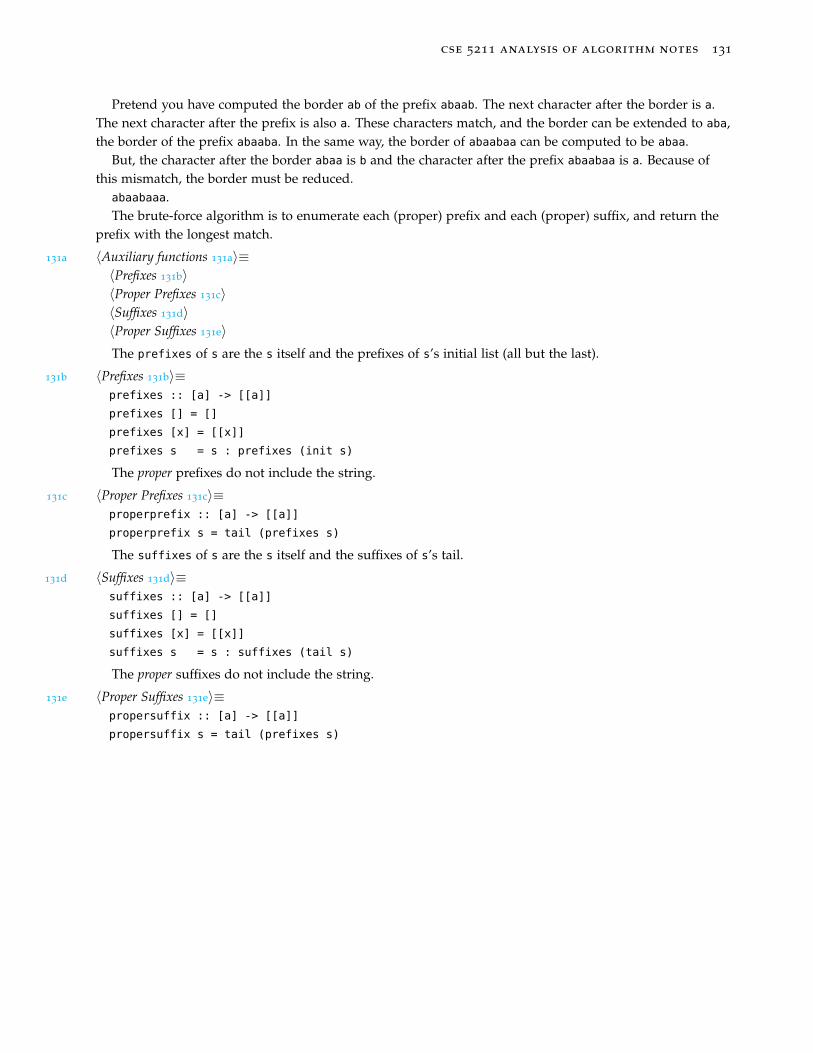
cse 5211 analysis of algorithm notes 131
Pretend you have computed the border ab of the prefix abaab. The next character after the border is a.The next character after the prefix is also a. These characters match, and the border can be extended to aba,the border of the prefix abaaba. In the same way, the border of abaabaa can be computed to be abaa.
But, the character after the border abaa is b and the character after the prefix abaabaa is a. Because ofthis mismatch, the border must be reduced.
abaabaaa.The brute-force algorithm is to enumerate each (proper) prefix and each (proper) suffix, and return the
prefix with the longest match.
131a 〈Auxiliary functions 131a〉≡〈Prefixes 131b〉〈Proper Prefixes 131c〉〈Suffixes 131d〉〈Proper Suffixes 131e〉The prefixes of s are the s itself and the prefixes of s’s initial list (all but the last).
131b 〈Prefixes 131b〉≡prefixes :: [a] -> [[a]]
prefixes [] = []
prefixes [x] = [[x]]
prefixes s = s : prefixes (init s)
The proper prefixes do not include the string.
131c 〈Proper Prefixes 131c〉≡properprefix :: [a] -> [[a]]
properprefix s = tail (prefixes s)
The suffixes of s are the s itself and the suffixes of s’s tail.
131d 〈Suffixes 131d〉≡suffixes :: [a] -> [[a]]
suffixes [] = []
suffixes [x] = [[x]]
suffixes s = s : suffixes (tail s)
The proper suffixes do not include the string.
131e 〈Proper Suffixes 131e〉≡propersuffix :: [a] -> [[a]]
propersuffix s = tail (prefixes s)
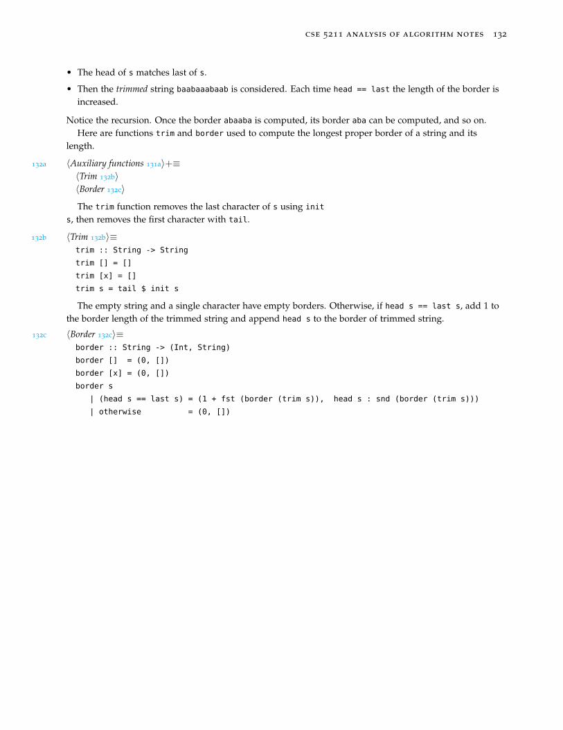
cse 5211 analysis of algorithm notes 132
• The head of s matches last of s.
• Then the trimmed string baabaaabaab is considered. Each time head == last the length of the border isincreased.
Notice the recursion. Once the border abaaba is computed, its border aba can be computed, and so on.Here are functions trim and border used to compute the longest proper border of a string and its
length.
132a 〈Auxiliary functions 131a〉+≡〈Trim 132b〉〈Border 132c〉
The trim function removes the last character of s using init
s, then removes the first character with tail.
132b 〈Trim 132b〉≡trim :: String -> String
trim [] = []
trim [x] = []
trim s = tail $ init s
The empty string and a single character have empty borders. Otherwise, if head s == last s, add 1 tothe border length of the trimmed string and append head s to the border of trimmed string.
132c 〈Border 132c〉≡border :: String -> (Int, String)
border [] = (0, [])
border [x] = (0, [])
border s
| (head s == last s) = (1 + fst (border (trim s)), head s : snd (border (trim s)))
| otherwise = (0, [])

cse 5211 analysis of algorithm notes 133
A border has a dual notion called period: An integer p, the shift needed to align the border. For instance,the borders and periods of s=abaabaaabaaba are 7, 10, 12, 13.
index 0 1 2 3 4 5 6 7 8 9 10 11 12
s a b a a b a a a b a a b ap=7 a b a a b a a b a a b ap=10 a b a a b ap=12 a ap=13
The last period 13 corresponds to the empty border. The invariant is
p + length (border s) = length s
Shifting a pattern by a period aligns borders. Such shifts are feasible, if they are safe.When a mismatch occurs shift, pattern by $p =$ (length s)-(length (border s)), the period of the
matched border. Here’s an example:
pattern index j 0 1 2 3 4 5pattern a b a a b atext a a b a c a b a a . . .text index i 0 1 2 3 4 5 6 7 8 . . .
The mismatch occurs at j=3 once we’ve matched aba, which has border a of length 1. The period of aba]is [[2. Shifting pattern 2 = 3− 1 positions produces an alignment of the border a of aba
pattern index j 0 1 2 3 4 5pattern a b a a b atext a a b a c a b a a . . .text index i 0 1 2 3 4 5 6 7 8 . . .
We can restart the matching at j=1=border[j]. We don’t need to recheck the match at pattern[0] withtext[3]. Of course there is an immediate mismatch at the next position, which is handled by Knuth’soptimization.