GNS Science

CSEP Developments in Support of Operational Earthquake Forecasting – a Future Perspective

David Rhoades Workshop on “Operational Earthquake Forecasting and Decision-making” Varenna, Italy, 8-11 June 2014

GNS Science

Hand with Reflecting Sphere - lithograph print by M. C. Escher, 1935

GNS Science

The usefulness of a standard CSEP model format

GNS Science

STEP NSHM

EEPAS PPE

24 hour

Forecasts

M≥5

converted from longer term rates

Models in the NZ testing centre

The usefulness of a standard CSEP model format

GNS Science

Current CSEP initiatives

•  Physics-based models: Retrospective tests of short-term models in the Canterbury earthquake sequence – including statistical aftershock models and Coulomb models (REAKT/CSEP).

•  High-resolution global experiment: Tests of annual and daily models on 0.1 degree pole-pole grid.

•  Heritage models: Global tests of M8 algorithm, with circular alarm regions and three-month updating, against a reference model.

•  Precursors: Encouragement to potential providers of earthquake alarms based on a variety of geophysical precursors to participate in CSEP (initially by providing External Forecasts or Predictions).

GNS Science

Refinement of CSEP tests -Common criticisms of current tests •  L-test is blunt because the model likelihood is strongly

correlated with the number of earthquakes: Resolution: conditional L-test (Werner et al., 2010) is sharper.

•  R-test is difficult to interpret. It is mostly a consistency test, not a model-comparison test. Resolution: T/W- tests are better comparison tests.

•  Real earthquake sequences are not Poisson, because of clustering. The negative binomial fits better to the number of earthquakes in successive time periods, especially when target magnitude threshold is low.

•  Some models are not Poisson (e.g., ETAS).

GNS Science

Real earthquake sequences are not Poisson

Possible partial resolutions: • Modellers agree to N-test based on Poisson distribution.

• Use negative binomial distribution for N-test – requires two parameters (to be specified in advance by CSEP?)

• Modellers specify the distribution for the N-test, when the model is submitted .

GNS Science

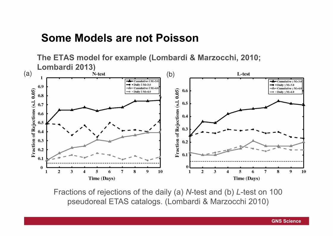
Some Models are not Poisson The ETAS model for example (Lombardi & Marzocchi, 2010; Lombardi 2013)

Fractions of rejections of the daily (a) N-test and (b) L-test on 100 pseudoreal ETAS catalogs. (Lombardi & Marzocchi 2010)

GNS Science

Some models are not Poisson

Possible partial resolutions • Use higher magnitude threshold for target events. • Use shorter update periods than one day, e.g., 30 minute testing in SCEC testing center. • Event-based testing with irregular updating periods (yet to be implemented). • Allow models to generate their own simulated catalogues, to be used in consistency tests. • Use alternative form of likelihood that has no regard to the numbers of earthquakes in individual cells.

GNS Science

Alternative likelihood function definitions

GNS Science

Efficiency of tests

•  The present simulation-based consistency tests threaten to outstrip available computing resources for large grids and/or frequent updating.

•  Computationally efficient alternative methods are available:

- streamlined simulations; - traditional large-sample approximations.

GNS Science

Efficient alternatives to existing CSEP simulation approach to consistency tests •  Distribution of bin rates is known from the forecast •  Distribution of earthquake-bin rates can be derived from it •  Could be well approximated by histograms of log bin-rates

Distribution of bin expectations and earthquake-bin expectations for one model (Rhoades et al. 2011)

GNS Science

Central limit theorem could be applied for conditional L-test, S-test etc. when N is “large” – how large?

Normal probability plot for conditional distribution, given the number of target earthquakes, N, of log likelihood of one CSEP model: (a) N = 1, (b) N = 2, (c) N = 8, and (d) N = 32. Solid line: from convolution of distributions, dotted line: from10,000 Monte Carlo simulations of target earthquakes. Dashed (diagonal) line: normal distribution. (Rhoades et al. 2011).

GNS Science

Central-Limit theorem convergence in T-test - bootstrap approach

95% confidence intervals for IGPE

95.6% according to bootstrap

c.f. Taroni et al. 2014

GNS Science

How large does N have to be for T-test to be trustworthy?

Assumed true distribution

True confidence level of “95% confidence interval for mean”,

i.e. percentage of intervals based on subsample of size N which

include the mean.

Derived from 10,000 independent samples of size N

GNS Science

Present and possible future CSEP systems

•  Present system •  Possible future system

Primary module:

Generates model forecasts and statistical summary for testing with automated running.

Testing module:

Performs tests based on forecasts, statistical summary and target earthquake rates.

Single module:

Generates model forecasts and performs standard set of tests on them with automated running. Little regard to efficiency of tests. Testing performed every time a model is updated.

GNS Science

Hybrid models: The way of the future Forming hybrids is one way to increase the information gain of forecasts. Sometimes the physics will demand complex hybrids, but some simple hybrids would be easily investigated in the CSEP system: Types of hybrid models • Additive hybrids

–  Protect against “blind-spots” of individual models • Maximum hybrids

–  Compensate for diminishing time-varying information with increasing time horizon

• Multiplicative hybrids –  Exploit independent information on earthquake occurrence held

by different models or data sets to ramp up probabilities in some cells.

GNS Science

Additive Hybrids - Protect against “blind-spots” of individual models

•  Forming normalised additive mixtures is easy, with continuous or discrete treatment of space and time.

•  Many existing models are actually additive hybrids

•  Examples: ETAS, EEPAS, STEP+EEPAS, etc

GNS Science

Additive hybrids (weighted average ensemble models)

Method Details References

Score model averaging (SMA) wi α 1/|Li|, Li: log-likelihood of model i .

Marzocchi et al. 2012., Taroni et al. 2014.

Generalised score model Averaging (gSMA)

wi α 1/(1+|Li-L0|), L0: log-likelihood of best model

Marzocchi et al. 2012., Taroni et al. 2014.

Bayes model averaging (BMA)

wi α δi exp(Li-L0), δi: correlation weight of model i.

Marzocchi et al. 2012.

Bayes factor model averaging (BMA)

wi α 1+βTBFi TBFi: total Bayes factor of model i.

Marzocchi et al. 2012., Taroni et al. 2014.

Parimutuel gambling model averaging (PGMA)

wi α 1+γVi Vi: parimutuel gambling score of model i.

Zechar & Zhuang 2012, Taroni et al. 2014.

Maximum likelihood weighting (MLW)

wi chosen to maximise likelihood of hybrid model.

Gerstenberger & Rhoades 2009, Rhoades 2013.

Additive hybrids usually outperform individual CSEP models.

GNS Science

Maximum hybrids - Compensate for diminishing time-varying information with increasing time horizon

•  Natural way to combine a static background model with a time-varying one.

•  Examples: 1. STEP (Gerstenberger et al.,

2005) 2. Canterbury operational

forecasting model (EE) (Gerstenberger et al., 2014)

•  Easy to manage in discrete space-time.

Ca

Canterbury EE model forecast for central

Christchurch

GNS Science

• 

Multiplicative hybrids •  Exploit independent information on earthquake

occurrence held by different models or data sets by ramping up probabilities in cells where “red spots” coincide.

•  Rooted in theory of multiple precursors in early papers by Aki, Utsu, et al.

•  Easier to manage in discrete space-time than continuous space, so well suited to CSEP model environment.

GNS Science

Rikitake (mid 1970’s)

GNS Science

Probability gains from unreliable precursors Aki(1981), Utsu (1983)

•  Streams of earthquakes E and precursors A,B,C,… (conditionally independent) in time

•  P(A∩B|E)=P(A|E)P(B|E), and same for Ē. •  Then showed (using Bayes rule) that if precursors

appear simultaneously

i.e. probability gain = product of individual probability gains

GNS Science

The Aki Strategy

GNS Science

The successful prediction of the Haicheng earthquake implies that the hazard rate (probability of occurrence per unit time) had been increased from about 1 per 1000 years to 1 per several hours through acquisition of precursory information. The probability gain at each of four stages of prediction is about a factor of 30.

Explanation of Haicheng success - Cao & Aki (1983)

GNS Science

Relaxation of independence assumption – Imoto (2007, 2010)

•  Relaxed conditional independence assumption for normally distributed case

•  Even if it doesn’t hold, still get multiplicative probability gains.

•  Instead allow for correlation between different precursors

•  Used the rate density of a model as a “surrogate precursor”, and showed how to combine EEPAS and b-value models, with multiplicative probability gains.

GNS Science

Pragmatic approaches – fitting multiplicative hybrids •  Weighted geometric mean of cell rates

•  Differential probability gain from Molchan diagram. (Shebalin et al., 2012; in press)

•  Fit multiplier as monotone increasing function of cell rate or alarm function value (Rhoades et al., submitted)

GNS Science

Differential probability gain (Shebalin et al., 2012)

•  Differential probability gain g estimated as local slope of Molchan diagram (miss rate, ν, versus alarm proportion, τ).

•  Translates from a function of τ to a function of alarm degree, A.

GNS Science

EASTR EEPAS EAST*EEPAS

Differential probability gain Ramping up of rates before El Mayor - Cucapah earthquakes

(Shebalin et al. 2014)

GNS Science

Original  models   Transforma0on  Cell  rate  -­‐>  mul0plier  

Hybrid  model  

Total cell rate A (summed over magnitudes)

Monotone increasing multiplier function (Rhoades et al., submitted)

GNS Science

Informa0on  gain  per  earthquake  (penalized  for  fiAed  parameters)  HKJ  compared  to  hybrid  models  

Models  for  whole  of  California   Models  for  southern  California  

NB.  Models  to  the  leK  of  the  zero  line  are  more  informa0ve  than  HKJ  Target  earthquakes:  Mainshocks  +  A5ershocks  

Monotone increasing Multiplier function

GNS Science

Building facilities for optimising hybrid models into the CSEP software would:

–  allow the best combined model from among those already submitted to be found;

–  allow alarm-function forecasts to be assessed by rolling them into likelihood models;

–  facilitate building of models based on various geophysical data and physical ideas;

–  advance the use of CSEP as a scientific tool to improve our knowledge of earthquake predictability.

GNS Science

Possible future CSEP system

Primary module:

Generates model forecasts and statistical summary for testing, with automated running. Restricted access

Testing module:

Performs tests based on forecasts, statistical summary and target earthquake rates.

Open access

Hybridization module:

Uses model forecasts, statistical summaries and catalogs to fit new hybrid models for future testing.

Open access