1

© CSIR 2015 All rights to the intellectual property and/or contents of this document remain vested in the CSIR. This document is issued for the sole purpose for which it is supplied. No part of this publication may be reproduced, stored in a retrieval system or transmitted, in any form or by means electronic, mechanical, photocopying, recording or otherwise without the express written permission of the CSIR. It may also not be lent, resold, hired out or otherwise disposed of by way of trade in any form of binding or cover than that in

which it is published.

Forecasts for electricity demand in South Africa (2014 – 2050) using the

CSIR sectoral regression model

January 2016

Project report Prepared for: Eskom

(as inputs into the IRP 2015)

Document Reference Number: CSIR/BE/SPS/ER/2015/0033/C CSIR Groupwise DMS: 257002 (Pta General Library) Project team leader: R Koen (012) 841-3045, rkoen@csir.co.za Project team members: JP Holloway, P Mokilane, S Makhanya, T Magadla, R Koen

2

Table of Contents 1. Introduction .................................................................................................................... 3 2. Methodology .................................................................................................................. 3

2.1. Data selection and use ........................................................................................... 3 2.1.1. Data on electricity consumption per sector ....................................................... 3 2.1.2. Data on losses ................................................................................................. 6 2.1.3. Data on drivers of electricity consumption ........................................................ 7

2.2. Regression model selection .................................................................................... 7 2.3. Adjustments for changes in electricity intensity ....................................................... 8

3. Forecasting results ....................................................................................................... 10 3.1. Forecasted driver values used .............................................................................. 10 3.2. Demand forecasts obtained .................................................................................. 16

4. Final remarks ............................................................................................................... 21 5. References .................................................................................................................. 21

List of Figures Figure 1 Comparing agricultural sector data between different sources ................................ 4 Figure 2 Comparing domestic sector data between different sources ................................... 4 Figure 3 Comparing commercial and manufacturing sector data between different sources . 5 Figure 4 Comparing mining sector data between different sources ....................................... 6 Figure 5 Comparing transport sector data between different sectors ..................................... 6 Figure 6 Model fitted for the electricity intensity “correction factor” ........................................ 9 Figure 7 Values used for electricity intensity ratio in scenarios ............................................ 16 Figure 8 Recommended forecasts for national consumption of electricity using the "CSIR model" ................................................................................................................................. 19 Figure 9 Forecasted values for the 5 electricity sectors ...................................................... 20

List of Tables Table 1 Sources for historical data on “drivers” of electricity consumption ............................. 7 Table 2 Summary of regression models used per sector ....................................................... 8 Table 3 Driver forecasts that were the same between different scenarios ........................... 10 Table 4 GDP % growth forecasts per scenario .................................................................... 11 Table 5 FCEH % growth forecasts per scenario .................................................................. 12 Table 6 Manufacturing index forecasts per scenario (base year = 2010) ............................. 13 Table 7 Forecasts for mining production index, excluding gold (base year = 2010) ............. 13 Table 8 Forecasts for gold ore treated (million metric tons) ................................................. 14 Table 9 National electricity demand: historical data and CSIR recommended forecasts (including adjustments for electricity intensity changes in the manufacturing sector) ........... 16

3

1. Introduction The CSIR developed a methodology for forecasting annual national electricity demand in collaboration with BHP Billiton in 2003. This methodology has subsequently been re-used in providing some of the forecasts used in the previous IRP and its revision. A set of forecasts have again been developed using this methodology, in conjunction with updated historical data covering the period 1990 – 2013, for producing forecasts for the IRP2015. These forecasts, and a brief description of the models used to derive the forecasts, are provided in this document. However, this document provides only brief references to the modelling approach, and the full methodology is not explained here. For more information on the methodological aspects and the process of developing the methodology, please refer to previous reports or to [1].

2. Methodology The methodology followed to obtain the forecasts presented in this document consisted of two parts. The first part consisted of putting together the required historical datasets to use as a basis for the set of forecasting models, and the second part consisted of compiling the models. Subsection 2.1 discusses the data-related task, while section 2.2 provides details on the set of forecasting models compiled.

2.1. Data selection and use

The data collection tasks involved the collection of electricity consumption data, the breakdown of this data per electricity usage sector, as well as the collection of data on the “drivers” of electricity consumption. The collection of the various types of data is discussed in the following sub-subsection, while the use of the “drivers” is explained in subsection 2.2.

2.1.1. Data on electricity consumption per sector Data from various sources had already been compared extensively during the process of developing the BHP Billiton forecasts, and further data comparisons were done during the forecasting for the previous IRP. Since the models developed require the most up-to-date historical data available, this round of forecasting again involved doing data collection, derivation and comparisons on the “new” historical data that were collected. Updated data on the electricity usage within the various electricity sectors were collected or derived. The sector breakdowns were checked by comparing the aggregated sector values to the national consumption figures published by Statistics SA in its P4141 series on electricity production volumes and sales, and adjusted where necessary. The sectors used in this report correspond to the categories used by the National Energy Regulator of South Africa (NERSA) that were also used by the Department of Energy, and reported to the International Energy Agency (see [2] for their 2007 statistics on electricity for South Africa, as well as [3] for a list of their data sources). It should be noted that NERSA has not published any data on electricity demand per sector since 2006, and the data published by the Department of Energy for their Energy Balances datasets did not seem to provide reliable data for the period since 2006. Although the Energy Balances are published per year, comparison of the sectoral electricity estimates over time indicated values that remained exactly the same for some of the sectors over three years, thus indicating data reliability issues. While Eskom publishes data broken down per sector in their Annual reports, sectoral breakdowns are only done for Eskom’s direct

4

customers. This leaves a large portion of the consumption belonging to the “Redistributor” sector which mainly represents municipalities (who in turn sell electricity to users within different sectors), and therefore needs to be broken down further into sectors. The CSIR team has received data from Eskom in which Eskom has done their own (complete) sector breakdown estimates for internal planning purposes, and these estimates were understood to be based on Eskom customer categories, but adjusted to national consumption in each sector by breaking down the redistributor component into the other categories using estimates of Eskom’s share in each category. However, the CSIR team used the Eskom estimates as comparative values only, and we compiled our own estimates of the sectoral breakdown values from a range of data sources. We also developed a new method to provide additional verification of the sector breakdowns, which is not discussed in this report (but details could be obtained from the CSIR project team, if required). The graphs in Figures 1 – 5, below, illustrate the comparative values per sector from the various data sources, and also show the “CSIR Recommended” sectoral breakdowns in comparison to the values from these other sources.

Figure 1 Comparing agricultural sector data between different sources

Although the agricultural sector is a small sector, Figure 1 indicates that the various sources differed quite widely on the pattern of consumption in this sector during the period 1990 – 2000, but that the sources are more in agreement since the mid 2000s.

Figure 2 Comparing domestic sector data between different sources

0

1000

2000

3000

4000

5000

6000

7000

GW

h

Agricultural Electricity Consumption

RAU

NERSA (Unadjusted)

DME Digest (2002)

DME Digest (1998)

DME (Energy Balances)

Recommended

Eskom's share

Estimate using Eskom %share

0

10000

20000

30000

40000

50000

60000

GW

h

Domestic Electricity Consumption

RAU

NERSA (Unadjusted)

DME Digest (2002)

DME Digest (1998)

DME (Energy Balances)

Recommended

Eskom share

Estimate using Eskom %share

5

For the domestic sector, the overall patterns between some sectors coincided, but generally the Eskom sector estimates were usually lower than other sources over the late 2000s. It is assumed that the estimates for this sector are problematic due to the fact that most of the domestic consumers are supplied with electricity via the municipalities, i.e. they form a large part of the “redistributors” sector within Eskom sales, and that relatively few domestic customers are direct Eskom customers.

Figure 3 Comparing commercial and manufacturing sector data between different

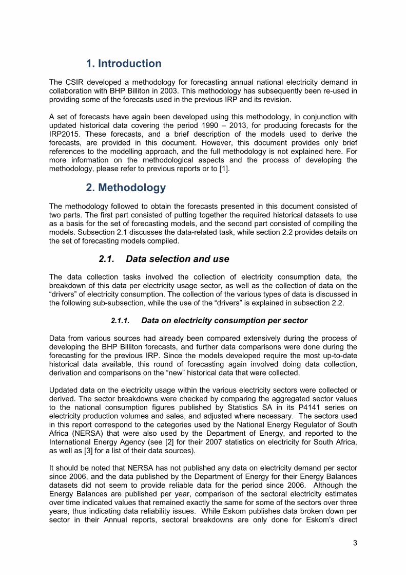
sources Although most sources provide separate “Commerce” and “Manufacturing” sectors, definitions differ widely between them, and even within different years of the same source. Furthermore, most sources contain a “general” category, and the definition of this category is also not consistent. However, when data on “commerce”, “manufacturing” and “general” sectors are combined for each of the various sources, the differences between the sources are not very substantial, as can be seen from Figure 3, and therefore the CSIR team prefers to combine these sectors into one. Figure 4 shows that the various sources do not differ very much in terms of the pattern for the mining sector. Since Eskom supplies most of this sector directly, in the years where differences occurred, the Eskom values were considered to be the more reliable source and hence the Eskom figures were used.

0

20000

40000

60000

80000

100000

120000

140000

160000

GW

h

Commerce+Manufacturing+General Electricity Consumption

RAU

NERSA (Unadjusted)

DME Digest (2002)

DME Digest (1998)

DME (Energy Balances)

Stats SA

Recommended

Eskom's share

Estimate using Eskom %share

6

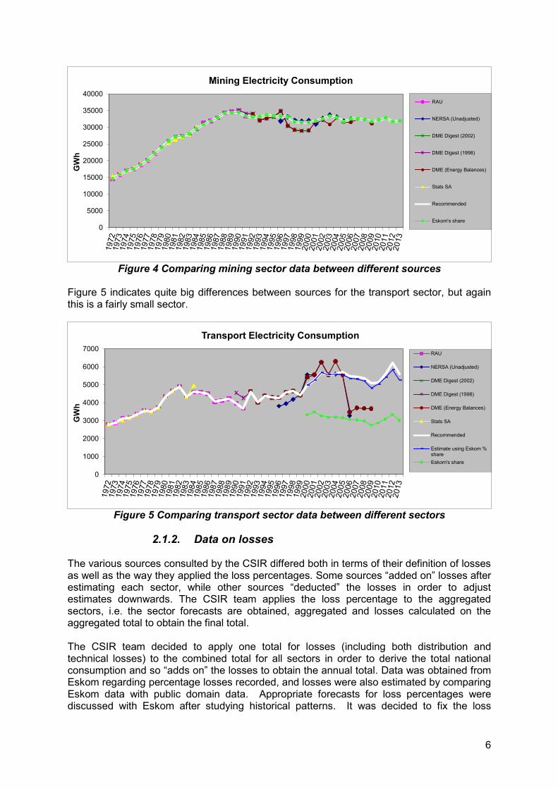
Figure 4 Comparing mining sector data between different sources

Figure 5 indicates quite big differences between sources for the transport sector, but again this is a fairly small sector.

Figure 5 Comparing transport sector data between different sectors

2.1.2. Data on losses

The various sources consulted by the CSIR differed both in terms of their definition of losses as well as the way they applied the loss percentages. Some sources “added on” losses after estimating each sector, while other sources “deducted” the losses in order to adjust estimates downwards. The CSIR team applies the loss percentage to the aggregated sectors, i.e. the sector forecasts are obtained, aggregated and losses calculated on the aggregated total to obtain the final total. The CSIR team decided to apply one total for losses (including both distribution and technical losses) to the combined total for all sectors in order to derive the total national consumption and so “adds on” the losses to obtain the annual total. Data was obtained from Eskom regarding percentage losses recorded, and losses were also estimated by comparing Eskom data with public domain data. Appropriate forecasts for loss percentages were discussed with Eskom after studying historical patterns. It was decided to fix the loss

0

5000

10000

15000

20000

25000

30000

35000

40000

GW

hMining Electricity Consumption

RAU

NERSA (Unadjusted)

DME Digest (2002)

DME Digest (1998)

DME (Energy Balances)

Stats SA

Recommended

Eskom's share

0

1000

2000

3000

4000

5000

6000

7000

GW

h

Transport Electricity ConsumptionRAU

NERSA (Unadjusted)

DME Digest (2002)

DME Digest (1998)

DME (Energy Balances)

Stats SA

Recommended

Estimate using Eskom %shareEskom's share

7

percentage at 11.5% for the entire forecasting period. This percentage corresponded with historical percentage fluctuations and, in discussion with Eskom staff, it was agreed that this value would be an estimate that would balance expansion of the transmission grid (i.e. increasing transmission losses) with changes in generation patterns (which may reduce other types of losses) over the medium to long term.

2.1.3. Data on drivers of electricity consumption For data on potential “drivers” of electricity, historical data were obtained from the South African Reserve Bank, Chamber of Mines and Statistics SA. The values for these “drivers” were compiled in consultation with Eskom in order to use a consistent base for the forecasts, for instance, ensuring that GDP figures and the various indices were standardised according to the same base year. Table 1 Sources for historical data on “drivers” of electricity consumption

“Driver” data Source Gross Domestic Product (GDP) Reserve Bank of South Africa Final Consumption Expenditure of Households (FCEH), also called Private Consumption Expenditure (PCE) in some sources

Reserve Bank of South Africa

Index for Manufacturing production volumes Statistics SA (Statistical releases) Index for Mining production volumes (gold, coal, iron ore, PGM and total index (including and excluding gold))

Statistics SA (Statistical releases)

Population Statistics SA (Midyear estimates) Number of households and average household size

Statistics SA (General Population Survey)

Gold ore milled and gold ore treated Chamber of Mines

2.2. Regression model selection

The methodology followed was to analyse data on electricity consumption as well as on aspects that describe general demographic and economic conditions which could conceivably influence consumption. Multiple regression modelling was chosen as the technique to be used for forecasting the annual consumption within the individual electricity sectors by relating such influencing aspects (or “drivers”) to the demand in each sector. The development of models for the different electricity consumption sectors involved identifying a big set of measures that could be considered as possible / potential predictors for each sector, followed by regression modelling to determine the best forecasting models for the consumption in each sector that could be obtained from this set. The modelling involved an iterative process of fitting a model, assessing it, making changes, rerunning and comparing the model to the one(s) before the changes. The “best” models were chosen from this iterative process to be statistically sound, to be as simple as possible (i.e. have as few “drivers” as possible), and to satisfy a logical understanding of the sector being forecasted. To know whether a model was statistically sound it had to show a good fit to the historical data, to have low levels of multi-collinearity and to show acceptable residual patterns. Model fit can be measured in various ways, but in this study the adjusted R2 value was used. The closer the adjuster R2 is to 1, the better the model fit. However, even models that fit the historical data well could suffer from high levels of multi-collinearity, so model fit alone is not sufficient. Multi-collinearity is the statistical term to indicate that the “drivers” included in the model are related to each other, and this can be

8

a problem in a model intended for forecasting. Models therefore had to have low levels of multi-collinearity to be considered acceptable. The levels of multi-collinearity of a regression model can be measured by the condition index (in this study the so-called singular-value decomposition condition index, with the centering option, as discussed on pp 337 – 341 in [4], was used) and the value of the condition index should be below 30 to ensure low levels of multi-collinearity. The CSIR team believes that the models derived for each sector fitted the collected historical data well and were also appropriate for forecasting future demand. Table 2 summarises the models (i.e., the group of CSIR models) used for each of the sectors’ forecasts. Data about the statistical fit of the models (as indicated by the adjusted R2), as well as the amount of multi-collinearity present in the model (as measured by the condition index), are given for each model.

Table 2 Summary of regression models used per sector Electricity sector

Model used (Note: the “predictor variables” indicated in bold in each model) Adjusted R2 Condition

index

Agriculture -47339 + 3725.82×ln(FCEH) Adjusted R2 = 0.97

N/A if only 1 variable in model

Transport 975.24 + 45.61×mining index excluding gold Adjusted R2 = 0.74

N/A if only 1 variable in model

Domestic -410694 + 31840×ln(FCEH) + 2339.48*recession Adjusted R2 = 0.97 CI = 1.4

Commerce & manufacturing

11000 + 0.02259×FCEH + 687.14368 × manufacturing index×correction factor (NOTE: The “correction factor” adjusts for electricity intensity as

explained in section 2.3 The intercept value was adjusted to align the starting point

of the forecasts (for 2014) with the observed actual values for 2014)

Adjusted R2 = 0.9691

CI = 21.27

Mining 21784 + 75.868× mining production index (excl. gold) + 0.05268×gold ore treated

Adjusted R2 = 0.55 CI = 6.3

Note that although CSIR was requested to use two different models in the commerce and manufacturing sector, one with and without the “correction factor”, the model fitted without the correction factors was not considered to be as good as the one with the “correction factor”, and therefore only one model was developed. The “correction factor” was modelled historically as explained in the next subsection, and used in the forecasts as explained in section 3.1.

2.3. Adjustments for changes in electricity intensity

The CSIR team has in the past (i.e. previously when a set of forecasts for electricity demand was developed) used the historical data as the main basis for developing forecasting models without adjusting either the historical data or the forecasts. The assumption has been that any changes with regard to electricity usage, such as responses to higher electricity prices, energy saving initiatives, and so on, would be recorded as part of the historical data, and therefore implicitly be factored into the models. However, for the previous revision of the IRP forecasts, a need was identified to add an explicit aspect regarding electricity intensity into the models for the manufacturing sector and not to rely only on the implicit incorporation of it based on historical patterns. This was considered necessary in order to provide a way to model future scenarios that contrast expansion of electricity intensive sectors of the economy with the development of less energy intensive sectors in order to achieve

9

economic growth. Therefore, the suggested scenario descriptions require that the future patterns of electricity intensity would differ from its historical patterns. In this new IRP forecast it was decided to continue this precedent, since there was again one scenario that involved the expansion of less energy intensive sectors. The way in which electricity intensity was added to the models was by incorporating a “correction factor” representing the ratio between electricity used and goods produced within, specifically, the manufacturing sector. Data on electricity usage within the manufacturing and commercial sector was taken from the Eskom estimates, and the ratio between this electricity usage and the index of manufacturing volumes (as obtained from Statistics SA) was calculated and plotted as indicated in Figure 6. The figure shows the historical pattern for the period 1994 – 2013 (corresponding to the period for which this specific data was available) with the purple line, and a polynomial curve fitted to this line to represent the overall trend in this ratio as the blue line. When the ratio decreases, then it indicates that less electricity was required to produce the same volume of goods, and when it increases then more electricity was used in order to produce similar volumes of goods. The estimated “correction factor” values, obtained from the polynomial curve, were used to represent a proxy for the historical trend in the electricity intensity in the manufacturing sector. The “correction factor” was multiplied with the manufacturing index and this combined variable was incorporated into the model (see Table 2 in section 2.2). In this way, the “correction factor” was used to adjust, or “correct”, the effect that the manufacturing index had on the electricity usage and therefore bring in some way of modelling the fact that less electricity seemed to have been used per unit produced.

Figure 6 Model fitted for the electricity intensity “correction factor”

10

3. Forecasting results This section provides the revised forecasts, namely demand forecasts for national consumption of electricity for the period 2014 – 2050.

3.1. Forecasted driver values used

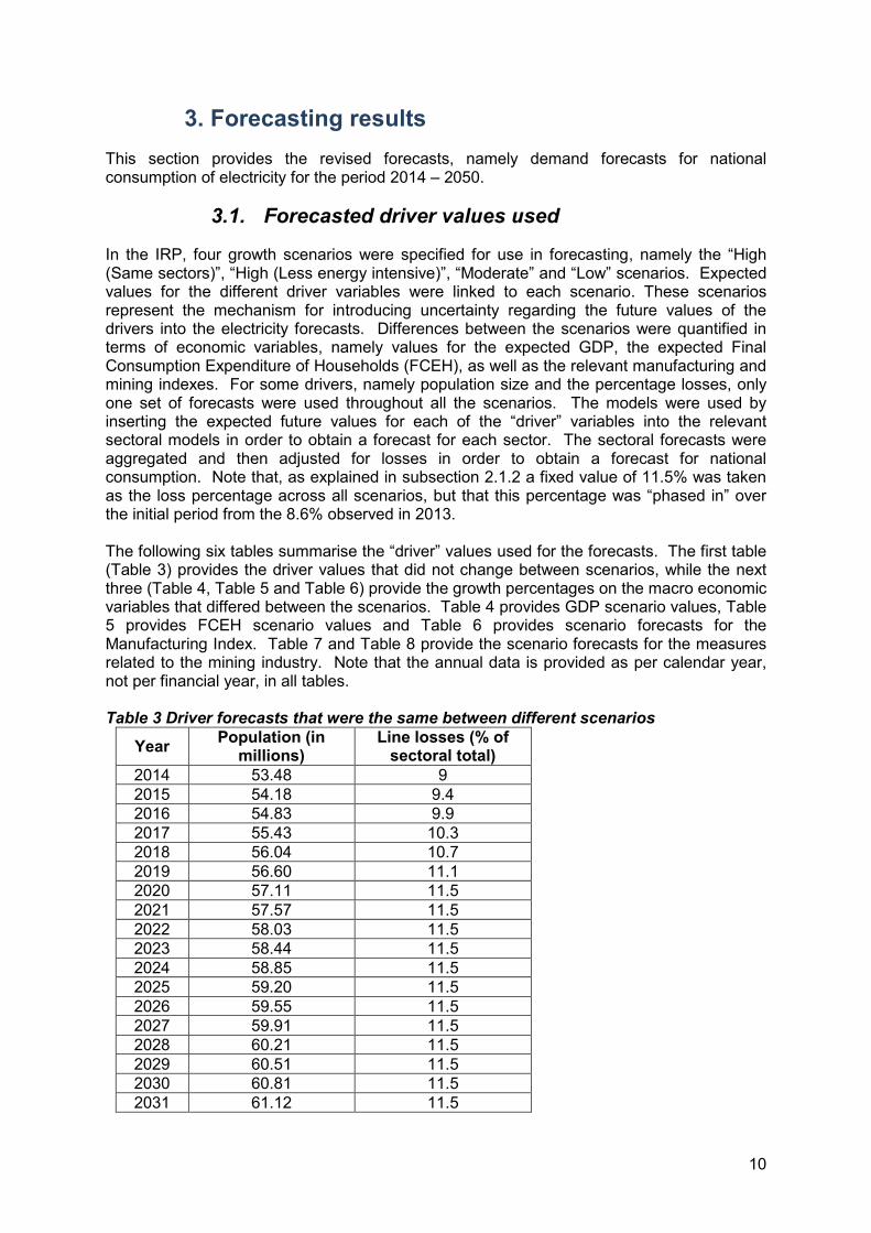
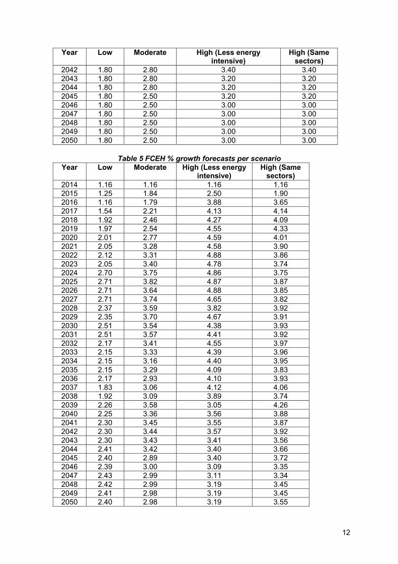
In the IRP, four growth scenarios were specified for use in forecasting, namely the “High (Same sectors)”, “High (Less energy intensive)”, “Moderate” and “Low” scenarios. Expected values for the different driver variables were linked to each scenario. These scenarios represent the mechanism for introducing uncertainty regarding the future values of the drivers into the electricity forecasts. Differences between the scenarios were quantified in terms of economic variables, namely values for the expected GDP, the expected Final Consumption Expenditure of Households (FCEH), as well as the relevant manufacturing and mining indexes. For some drivers, namely population size and the percentage losses, only one set of forecasts were used throughout all the scenarios. The models were used by inserting the expected future values for each of the “driver” variables into the relevant sectoral models in order to obtain a forecast for each sector. The sectoral forecasts were aggregated and then adjusted for losses in order to obtain a forecast for national consumption. Note that, as explained in subsection 2.1.2 a fixed value of 11.5% was taken as the loss percentage across all scenarios, but that this percentage was “phased in” over the initial period from the 8.6% observed in 2013. The following six tables summarise the “driver” values used for the forecasts. The first table (Table 3) provides the driver values that did not change between scenarios, while the next three (Table 4, Table 5 and Table 6) provide the growth percentages on the macro economic variables that differed between the scenarios. Table 4 provides GDP scenario values, Table 5 provides FCEH scenario values and Table 6 provides scenario forecasts for the Manufacturing Index. Table 7 and Table 8 provide the scenario forecasts for the measures related to the mining industry. Note that the annual data is provided as per calendar year, not per financial year, in all tables. Table 3 Driver forecasts that were the same between different scenarios

Year Population (in millions)

Line losses (% of sectoral total)

2014 53.48 9 2015 54.18 9.4 2016 54.83 9.9 2017 55.43 10.3 2018 56.04 10.7 2019 56.60 11.1 2020 57.11 11.5 2021 57.57 11.5 2022 58.03 11.5 2023 58.44 11.5 2024 58.85 11.5 2025 59.20 11.5 2026 59.55 11.5 2027 59.91 11.5 2028 60.21 11.5 2029 60.51 11.5 2030 60.81 11.5 2031 61.12 11.5

11

Year Population (in millions)

Line losses (% of sectoral total)

2032 61.42 11.5 2033 61.73 11.5 2034 62.04 11.5 2035 62.35 11.5 2036 62.66 11.5 2037 62.97 11.5 2038 63.29 11.5 2039 63.61 11.5 2040 63.92 11.5 2041 64.24 11.5 2042 64.56 11.5 2043 64.89 11.5 2044 65.21 11.5 2045 65.54 11.5 2046 65.87 11.5 2047 66.19 11.5 2048 66.53 11.5 2049 66.86 11.5 2050 67.19 11.5

Table 4 GDP % growth forecasts per scenario

Year Low Moderate High (Less energy intensive)

High (Same sectors)

2014 1.57 1.57 1.57 1.57 2015 1.40 2.20 2.50 2.50 2016 1.40 2.30 3.50 3.50 2017 1.80 2.70 4.00 4.00 2018 2.00 2.90 4.20 4.20 2019 2.00 3.00 4.50 4.50 2020 2.00 3.20 4.50 4.50 2021 2.20 3.50 4.50 4.50 2022 2.20 3.50 4.50 4.50 2023 2.20 3.60 4.50 4.50 2024 2.40 3.80 4.50 4.50 2025 2.40 3.80 4.50 4.50 2026 2.40 3.70 4.50 4.50 2027 2.40 3.70 4.30 4.30 2028 2.20 3.60 4.30 4.30 2029 2.20 3.60 4.30 4.30 2030 2.20 3.50 4.10 4.10 2031 2.20 3.50 4.10 4.10 2032 2.00 3.40 4.10 4.10 2033 2.00 3.30 4.00 4.00 2034 2.00 3.20 4.00 4.00 2035 2.00 3.20 3.80 3.80 2036 2.00 3.00 3.80 3.80 2037 1.80 3.00 3.80 3.80 2038 1.80 3.00 3.60 3.60 2039 1.80 3.00 3.60 3.60 2040 1.80 2.80 3.40 3.40 2041 1.80 2.80 3.40 3.40

12

Year Low Moderate High (Less energy intensive)

High (Same sectors)

2042 1.80 2.80 3.40 3.40 2043 1.80 2.80 3.20 3.20 2044 1.80 2.80 3.20 3.20 2045 1.80 2.50 3.20 3.20 2046 1.80 2.50 3.00 3.00 2047 1.80 2.50 3.00 3.00 2048 1.80 2.50 3.00 3.00 2049 1.80 2.50 3.00 3.00 2050 1.80 2.50 3.00 3.00

Table 5 FCEH % growth forecasts per scenario

Year Low Moderate High (Less energy intensive)

High (Same sectors)

2014 1.16 1.16 1.16 1.16 2015 1.25 1.84 2.50 1.90 2016 1.16 1.79 3.88 3.65 2017 1.54 2.21 4.13 4.14 2018 1.92 2.46 4.27 4.09 2019 1.97 2.54 4.55 4.33 2020 2.01 2.77 4.59 4.01 2021 2.05 3.28 4.58 3.90 2022 2.12 3.31 4.88 3.86 2023 2.05 3.40 4.78 3.74 2024 2.70 3.75 4.86 3.75 2025 2.71 3.82 4.87 3.87 2026 2.71 3.64 4.88 3.85 2027 2.71 3.74 4.65 3.82 2028 2.37 3.59 3.82 3.92 2029 2.35 3.70 4.67 3.91 2030 2.51 3.54 4.38 3.93 2031 2.51 3.57 4.41 3.92 2032 2.17 3.41 4.55 3.97 2033 2.15 3.33 4.39 3.96 2034 2.15 3.16 4.40 3.95 2035 2.15 3.29 4.09 3.83 2036 2.17 2.93 4.10 3.93 2037 1.83 3.06 4.12 4.06 2038 1.92 3.09 3.89 3.74 2039 2.26 3.58 3.05 4.26 2040 2.25 3.36 3.56 3.88 2041 2.30 3.45 3.55 3.87 2042 2.30 3.44 3.57 3.92 2043 2.30 3.43 3.41 3.56 2044 2.41 3.42 3.40 3.66 2045 2.40 2.89 3.40 3.72 2046 2.39 3.00 3.09 3.35 2047 2.43 2.99 3.11 3.34 2048 2.42 2.99 3.19 3.45 2049 2.41 2.98 3.19 3.45 2050 2.40 2.98 3.19 3.55

13

Table 6 Manufacturing index forecasts per scenario (base year = 2010)

Year Low Moderate High (Less energy intensive)

High (Same sectors)

2014 106.4 106.4 106.4 106.4 2015 107.5 108.6 108.0 109.1 2016 108.6 111.3 110.2 111.8 2017 110.2 114.6 112.4 115.2 2018 111.9 118.3 115.2 119.2 2019 113.5 122.3 118.7 124.0 2020 115.2 126.7 122.2 129.9 2021 117.5 131.3 125.9 136.4 2022 119.9 136.3 129.7 143.5 2023 122.3 141.4 133.6 151.0 2024 124.1 146.8 137.3 158.8 2025 126.0 152.4 141.1 166.8 2026 127.9 158.2 145.1 175.1 2027 129.8 163.9 148.9 183.0 2028 131.7 169.8 152.7 191.2 2029 133.7 175.5 156.7 199.8 2030 135.3 181.5 160.8 208.2 2031 136.9 187.7 164.8 217.0 2032 138.6 194.1 168.4 226.1 2033 140.3 200.3 172.1 235.1 2034 141.9 206.7 175.9 244.5 2035 143.6 212.9 179.8 253.3 2036 145.4 219.3 183.7 261.9 2037 147.1 225.4 187.8 270.9 2038 148.6 231.7 191.5 280.1 2039 150.1 237.7 195.4 289.0 2040 151.6 243.5 199.3 298.3 2041 153.1 248.8 203.3 307.8 2042 154.6 254.3 207.3 317.7 2043 156.2 259.9 211.5 327.8 2044 157.4 265.6 215.7 337.7 2045 158.7 271.4 220.0 347.8 2046 159.9 276.9 224.4 358.2 2047 161.2 282.4 228.9 369.0 2048 162.5 288.1 233.0 379.3 2049 163.8 293.8 237.2 389.9 2050 165.1 299.7 241.5 400.1

Table 7 Forecasts for mining production index, excluding gold (base year = 2010)

Year Low Moderate High (Less energy intensive)

High (Same sectors)

2014 102.7 102.7 102.7 102.7 2015 105.3 105.9 106.1 106.6 2016 108.1 109.4 109.7 110.7 2017 110.9 112.8 113.0 115.9 2018 113.7 116.2 116.4 122.4 2019 116.4 119.8 119.7 129.3 2020 119.0 123.5 123.1 136.0 2021 121.6 127.1 126.5 143.0

14

Year Low Moderate High (Less energy intensive)

High (Same sectors)

2022 124.2 130.8 129.8 150.5 2023 127.0 134.5 133.1 158.3 2024 129.5 138.3 136.5 166.2 2025 132.1 142.0 139.9 174.3 2026 134.7 145.7 143.2 182.9 2027 137.3 149.5 146.6 191.5 2028 139.9 153.3 149.8 199.6 2029 142.5 157.1 153.1 208.1 2030 145.2 160.9 156.2 215.1 2031 147.9 164.6 159.3 222.4 2032 150.6 168.2 162.1 229.4 2033 153.4 171.8 165.1 236.2 2034 156.2 175.5 167.9 243.1 2035 159.1 179.1 170.7 250.3 2036 161.9 182.7 173.4 257.7 2037 164.7 186.2 175.9 264.0 2038 167.6 189.5 178.4 270.0 2039 170.5 192.8 181.0 276.0 2040 173.4 196.1 183.5 282.3 2041 176.0 199.4 186.1 288.6 2042 178.6 202.8 188.5 294.4 2043 181.1 206.2 191.0 300.3 2044 183.6 209.7 193.5 306.3 2045 186.1 213.3 196.0 311.6 2046 188.6 216.7 198.6 317.1 2047 190.7 220.2 200.8 322.6 2048 192.8 223.8 203.1 328.3 2049 195.0 227.4 205.4 334.0 2050 197.2 231.1 207.8 339.9

Table 8 Forecasts for gold ore treated (million metric tons)

Year Low Moderate High (Less energy intensive)

High (Same sectors)

2014 41.6 41.6 41.6 41.6 2015 40.4 41.0 40.4 41.4 2016 39.2 40.4 39.2 41.2 2017 38.4 39.8 38.4 41.0 2018 37.6 39.4 37.6 40.8 2019 36.9 39.0 36.9 40.6 2020 36.1 38.6 36.1 40.4 2021 35.6 38.6 35.4 40.2 2022 35.0 38.6 34.7 40.0 2023 34.7 38.6 34.0 39.8 2024 34.3 38.6 33.3 39.8 2025 34.0 38.6 32.7 39.8 2026 33.8 38.6 32.0 39.8 2027 33.7 38.6 31.4 39.8 2028 33.5 38.6 30.7 39.8 2029 33.5 38.6 30.1 39.8 2030 33.5 38.6 29.5 39.8 2031 33.5 38.6 28.9 39.8

15

Year Low Moderate High (Less energy intensive)

High (Same sectors)

2032 33.5 38.6 28.6 39.8 2033 33.5 38.6 28.3 39.8 2034 33.5 38.6 28.1 39.8 2035 33.5 38.6 27.8 39.8 2036 33.5 38.6 27.5 39.8 2037 33.5 38.6 27.2 39.8 2038 33.5 38.6 27.0 39.8 2039 33.5 38.6 27.0 39.8 2040 33.5 38.6 27.0 39.8 2041 33.5 38.6 27.0 39.8 2042 33.5 38.6 27.0 39.8 2043 33.5 38.6 27.0 39.8 2044 33.5 38.6 27.0 39.8 2045 33.5 38.6 27.0 39.8 2046 33.5 38.6 27.0 39.8 2047 33.5 38.6 27.0 39.8 2048 33.5 38.6 27.0 39.8 2049 33.5 38.6 27.0 39.8 2050 33.5 38.6 27.0 39.8

Since the “High (less energy intensive)” scenario has the same GDP growth as the “High (same sectors)” scenario but with the growth happening not in the mining and manufacturing economic sectors but rather in the tertiary economic sector, it was therefore considered important to distinguish between the electricity usage of the two scenarios by way of the “correction factor”. Therefore, for the “High (less energy intensive)” scenario a pattern was forecasted for future values of the “correction factor” as illustrated with the purple line in Figure 7, while for the other scenarios it was kept at a constant rate. The constant rate is illustrated with the red line in Figure 7. The two sets of forecasted values are compared with the historical pattern (the green line in Figure 7), which was also seen in Figure 6.

16

Figure 7 Values used for electricity intensity ratio in scenarios

3.2. Demand forecasts obtained

The forecasts obtained for each of the four scenarios are provided in Table 9 below. Note that the forecasts in Table 9 include the adjustments for energy intensity improvements in the manufacturing sector, as applicable to each scenario, by way of the “correction factor”.

Table 9 National electricity demand: historical data and CSIR recommended forecasts (including adjustments for electricity intensity changes in the manufacturing sector)

Year Annual electricity demand forecasts (GWh) per scenario, provided per

calendar year:

Low Moderate High (Less energy intensive)

High (Same sectors)

2014 233758 233758 232960 233758

2015 236697 238080 236609 238623

2016 239850 243070 242087 245304

2017 243547 248694 247650 252907

2018 247628 254859 253855 261249

2019 251801 261430 260834 270539

2020 256046 268576 268029 280541

2021 259902 275428 274910 289988

0

0.2

0.4

0.6

0.8

1

1.21

99

0

19

93

19

96

19

99

20

02

20

05

20

08

20

11

20

14

20

17

20

20

20

23

20

26

20

29

20

32

20

35

20

38

20

41

20

44

20

47

20

50

Electricity intensity factor forecasts

Recorded historicaldata

Historical pattern(Polynomial curvefitted)

Constant intensityforecasted

Decreasing intensityforecasted

17

Year

Annual electricity demand forecasts (GWh) per scenario, provided per calendar year:

Low Moderate High (Less energy intensive)

High (Same sectors)

2022 263889 282669 282225 299978

2023 267885 290203 289637 310258

2024 272070 298301 297165 320945

2025 276335 306669 304899 331945

2026 280665 315114 312848 343373

2027 285060 323691 320573 354544

2028 289188 332340 327484 366115

2029 293360 341108 335590 378108

2030 297459 349934 343528 389904

2031 301615 359008 351929 402093

2032 305476 368140 360417 414713

2033 309372 377162 368926 427371

2034 313318 386208 377663 440451

2035 317317 395331 386186 453094

2036 321370 404242 394923 465922

2037 325100 413196 403895 479159

2038 328761 422375 412504 492268

2039 332855 432104 419956 506150

2040 337000 441394 428431 519879

2041 341200 450679 437330 533998

2042 345452 460169 446452 548543

2043 349756 469867 455517 562902

2044 354006 479779 464786 577384

2045 358306 489102 474278 592283

2046 362657 498374 483382 606936

2047 367061 507833 492690 621979

2048 371517 517484 502095 637116

18

Year

Annual electricity demand forecasts (GWh) per scenario, provided per calendar year:

Low Moderate High (Less energy intensive)

High (Same sectors)

2049 376027 527331 511716 652657

2050 380591 537379 521559 668272

The CSIR recommended forecasts obtained for all four of the scenarios are illustrated graphically in Figure 8, while the forecasts for the five sectors making up the total consumption are provided in five separate graphs in Figure 9.

19

Figure 8 Recommended forecasts for national consumption of electricity using the "CSIR model"

20

Figure 9 Forecasted values for the 5 electricity sectors

21

4. Final remarks The “CSIR model” forecasts the national demand for electricity at a macro level, based on data relating to macro level economic and demographic indicators. The set of forecasts presented in this report were obtained using the methodology and scenarios as described to produce a set of forecasts as inputs into the IRP 2015 process.

5. References [1] Koen, R., Holloway, J.P., 2014, Application of multiple regression analysis to

forecasting South Africa’s electricity demand, Journal of Energy in Southern Africa (JESA), Vol 25, No 4, November 2014.

[2] Website of the International Energy Agency (iea), at the specific address

http://www.iea.org/stats/electricitydata.asp?COUNTRY_CODE=ZA [accessed September 2012]

[3] Website of the International Energy Agency (iea), at the specific address

http://wds.iea.org/wds/pdf/documentation_wedbes.pdf, pp 70 – 71 [accessed September 2012]

[4] Montgomery, D.C., Peck, E.A., Vining, G.G., 2006, Introduction to linear regression

analysis (Ed 4), John Wiley & Sons Inc.