CT Image Reconstruction Basics 1. Introduction CT perfusion imaging requires the reconstruction of a series of time-dependent volumetric datasets. The sequence of CT volumes measures the dynamics of contrast agent both in the vasculature and in the parenchyma. CT image reconstruction refers to the computational process of determining tomographic images from X-ray projection images of the irradiated patient. Image reconstruction is a compute-intensive task and one of the most crucial steps in the CT imaging process. As the basics of X-ray physics were detailed in Chapter 1, we assume that the result of the X-ray image formation is an attenuation image. Each individual pixel on the detector therefore represents a line integral, that is, the accumulation of all X-ray attenuation coefficients along the projection line. Here, the projection line is the connecting line of the X-ray focal spot with the center of the respective detector pixel. 2. From Line Integrals to Voxels In spite of the discrete nature of the projection images, most reconstruction theory uses a continuous framework, in which the reconstruction algorithms are derived mathematically. The problem of discrete sampling is then solved within the final formulation of the reconstruction algorithm. As the discrete sampling is a more technical issue, we will neglect it here for the ease of presentation and refer to the literature that details these steps [1]. Thus, we will remain in a continuous domain in this section. a. Radon Transform

Figure 1: Parallel-beam geometry and the generation of a parallel-beam projection 𝒑(𝒔,𝜽).

For ease of understanding, we explain the approach in the 2D (x,y) plane. The source-detector arrangement is rotating around the object (Figure 1). In the following, we will use Dirac’s 𝛿-function to select the parts of the object that are traversed by the X-ray. Recall that 𝛿 (t) is zero everywhere except at t=0, where 𝛿 becomes infinite. Furthermore, the 𝛿 -function fulfills for any real-valued function 𝑔(𝑥) the shifting property:

� 𝑔(𝑥)∞

−∞𝛿(𝑥 − 𝑥0)d𝑥 = 𝑔(𝑥0)

A parallel projection 𝑝(𝑠,𝜃) at detector element 𝑠 and at source/detector array rotation angle 𝜃 can be written in the following notation:

𝑝(𝑠,𝜃) = � ∞

−∞� 𝑓(𝑥,𝑦)𝛿(𝑥 cos 𝜃 + 𝑦 sin𝜃 − 𝑠)d𝑥 d𝑦∞

−∞,

where 𝑓(𝑥,𝑦) represents the X-ray attenuation coefficient at object location (𝑥,𝑦). Thus, the 𝛿-function selects the line 𝑥 cos 𝜃 + 𝑦 sin𝜃 = 𝑠 that connects the detector and the source array at 𝑠 while both arrays are rotated by 𝜃. Thus, 𝑝(𝑠,𝜃) describes a line integral whose value is observed at the detector. This process of turning function values 𝑓(𝑥,𝑦) into line integral values 𝑝(𝑠,𝜃) is also referred to as the Radon transform in 2D. The fundamental problem of CT reconstruction is the computation of function values 𝑓(𝑥, 𝑦) from the measured line integral values 𝑝(𝑠,𝜃); i.e., the inverse Radon transform. Another important concept in CT reconstruction is back-projection, as we will see in the following. A back-projection is a kind of conjugate (but not inverse) process to the (forward) projection. For the case of parallel-beam X-ray projections, it assigns to a point (𝑥,𝑦) in object coordinates the integral 𝑏(𝑥,𝑦) of the projection values that lie on the X-rays passing through (𝑥,𝑦):

𝑏(𝑥,𝑦) = �𝑝𝜋

0

(𝑠, 𝜃) �|𝑠=𝑥 cos𝜃+𝑦 sin𝜃𝑑𝜃.

b. Fourier Slice Theorem The Fourier Slice Theorem is fundamental to many CT reconstruction approaches. It states that the 1-D Fourier transform 𝑃(𝜔,𝜃) of a projection p(s, θ) in parallel-beam geometry for a fixed rotation angle 𝜃 is identical to the 1-D profile through the origin of the 2-D Fourier transform 𝐹(𝜔 cos 𝜃,𝜔 sin𝜃) of the irradiated object (𝑥,𝑦) . Figure 2 displays this process.

Figure 2: Illustration of the Fourier Slice Theorem.

c. Filtered Back-Projection for 2D Parallel-Beam Geometry With the Fourier Slice Theorem, we are able to elegantly derive one of the most commonly used reconstruction algorithms; the filtered back-projection (FBP) method. A derivation is shown in Technical Box 2. The resulting algorithm uses two concepts: Filtering and back-projection. The filter ℎ(𝑠) is called ramp filter because of the shape of |𝜔|. This filter corrects the oversampling that occurs in the center of the Fourier space. This is accomplished by enhancing high frequency components while dampening low frequency components. In practice, this filtering operation is often combined with additional filtering to achieve certain image characteristics. Various kernels can be created and embedded into the reconstruction process to obtain smoother or sharper images. After filtering, the projection data is back-projected into image space as described in the previous section. Note that the FBP algorithm uses the Fourier Slice Theorem only implicitly. Both filtering and back-projection can be implemented in a way that the actual computation of the Fourier Transform is not required. However, as the ramp filter is a global operation, and implementation using fast Fourier methods is often favorable.

𝑃(𝜔,𝜃) = � 𝑝(𝑠,𝜃)𝑒−2𝜋𝑖𝜔𝑠∞

−∞d𝑠.

𝑃(𝜔,𝜃) = � � 𝑓(𝑥,𝑦)𝛿(𝑥 cos 𝜃 + 𝑦 sin𝜃 − 𝑠)d𝑥d𝑦∞

−∞

∞

−∞ 𝑒−2𝜋𝑖𝜔𝑠d𝑠.

𝑃(𝜔,𝜃) = � 𝑓(𝑥,𝑦)� 𝛿(𝑥 cos 𝜃 + 𝑦 sin𝜃 − 𝑠)∞

−∞ 𝑒−2𝜋𝑖𝜔𝑠d𝑠d𝑥d𝑦,

∞

−∞

𝑃(𝜔,𝜃) = � 𝑓(𝑥,𝑦)𝑒−2𝜋𝑖(𝑥 cos𝜃+𝑦 sin𝜃)𝜔d𝑥d𝑦∞

−∞.

𝑃(𝜔,𝜃) = � 𝑓(𝑥,𝑦)𝑒−2𝜋𝑖(𝑥𝑢+𝑦𝑣) �|𝑢=ωcos𝜃, 𝑣=𝜔 sin𝜃d𝑥d𝑦∞

−∞,

𝑃(𝜔,𝜃) = 𝐹(𝜔 cos 𝜃,𝜔 sin 𝜃) = 𝐹𝑝𝑜𝑙𝑎𝑟(𝜔, 𝜃).

Technical Box 1: Fourier Slice Theorem Proof In order to prove this, we start with the 1-D Fourier transform 𝑃(𝜔, 𝜃) of 𝑝(𝑠, 𝜃):

Using the definition of the projection 𝑝(𝑠,𝜃) from above, we obtain

Rearranging the order of the integrals then yields

which, after elimination of the delta function, reads as

Finally, using the definition of the 2-D Fourier transform, we obtain

which results in the proposed statement

By varying 𝜃, we get the complete Fourier transform 𝐹polar(𝜔,𝜃) of the unknown function 𝑓(𝑥,𝑦) in polar coordinates (𝜔,𝜃).

d. Acquisition Geometries The filtered back-projection algorithm is an efficient and robust method for the computation of tomographic slice images. Using a fan-beam geometry based on a single X-ray source that is collimated towards a curved array of detector elements, it is possible to circumvent long acquisition times and bulky hardware that would be required for parallel-beam geometry. Doing so, a single source is sufficient to collect multiple rays at the same time (cf. Figure 2), but the Fourier Slice Theorem cannot be applied straightforwardly.

Figure 2: With fan-beam geometry, one is able to image multiple detector elements at the same time with only one X-ray source. Depending on the type of detector, two different geometries emerge. Using a curved

𝑓(𝑥,𝑦) = � � 𝐹 (𝑢, 𝑣)𝑒2𝜋𝑖(𝑢𝑥+𝑣𝑦) d𝑢d𝑣∞

−∞

∞

−∞

𝑓(𝑥,𝑦) = � � 𝐹polar(𝜔,𝜃)|𝜔|𝑒2𝜋𝑖𝜔(𝑥 cos𝜃+𝑦 sin𝜃) d𝜔d𝜃∞

−∞.

𝜋

0

𝑓(𝑥,𝑦) = � � 𝑃(𝜔,𝜃) |𝜔| 𝑒2𝜋𝑖𝜔(𝑥 cos𝜃+𝑦 sin𝜃) d𝜔 d𝜃∞

−∞

𝜋

0,

𝑓(𝑥,𝑦) = � 𝑝(𝑠,𝜃) ∗ ℎ(𝑠) �|𝑠=𝑥 𝑐𝑜𝑠𝜃+𝑦 sin𝜃d𝜃𝜋

0,

Technical Box 2: Derivation of the Filtered Back-Projection Algorithm In order to illustrate this derivation, we start with the inverse Fourier transform 𝐹 (𝑢, 𝑣):

and rewrite it to polar coordinates 𝐹polar(𝜔,𝜃) [34]:

According to the Fourier Slice Theorem, we obtain

which contains a product of the projection in 1D Fourier space 𝑃(𝜔,𝜃) and |𝜔|. The inverse Fourier transform of 𝑃(𝜔,𝜃) ⋅ |𝜔| corresponds to a convolution in spatial domain. The inverse Fourier transform of |𝜔| shall be defined by the filter kernel ℎ(𝑠). Hence, in spatial domain, the previous equation can then be written as

which is the back-projection of the projection data 𝑝(𝑠,𝜃) convolved with ℎ(𝑠).

detector an equiangular geometry described by 𝒈(𝜸,𝜷) is obtatined (left side) and using a linear detector an equally spaced geometry denoted by 𝒈(𝒕,𝜷) is created (right side).

If a full rotation with either parallel-beam or fan-beam acquisition geometries is performed, one can easily observe that both geometries cover identical data. They are merely collected in a different sequence. If we consider 𝛽 as the rotation angle of source and detector, 𝛾 as the angle to the respective detector elements, and 𝐷 as the source-to-rotation axis distance, the following relations between identical rays in fan-beam and parallel-beam geometry are obtained:

𝜃 = 𝛾 + 𝛽 (rays) 𝑠 = 𝐷 sin 𝛾

This relation offers two possible solutions for image reconstruction. Either the projection data is reordered into parallel-beam geometry in a so-called rebinning step, or the reconstruction algorithm has to be adapted to the acquisition geometry. Both algorithms are used in practice. The interpolation operation in the rebinning step must be handled with caution as it may lead to an unintended loss in image resolution. Technical Box 3 sketches an idea how to obtain an algorithm without rebinning.

𝑓(𝑥,𝑦) = 12�

1(𝐷′)2

2𝜋

0� 𝑔(𝛾,𝛽) ⋅

𝐷2�

𝛾′ − 𝛾sin(𝛾′ − 𝛾)

�2

ℎ(𝛾′ − 𝛾) cos 𝛾 d𝛾d𝛽.𝜋/2

−𝜋/2

𝑓(𝑥,𝑦) =12� 2𝜋

0

1(𝑈′)2

�𝐷

√𝐷2 + 𝑡2𝑔(𝑡,𝛽) ⋅ ℎ(𝑡′ − 𝑡) d𝑡d𝛽

∞

−∞.

Technical Box 3: Fan-Beam Reconstruction without Rebinning In order to omit rebinning, one has to reshape the filtered back-projection reconstruction formula by a change of coordinates of the integral variables 𝑠 and 𝜃 according to the ray identities in Eq. (rays). This yields the following fan-beam reconstruction formula:

Note that we introduced the variables 𝐷’ = 𝐷′(𝑥,𝑦,𝛽) and 𝛾′ = 𝛾’(𝑥,𝑦,𝛽) that describe distance and angle of the reconstructed point (𝑥, 𝑦) as shown in Figure 2. The equation above can be interpreted as a convolution of the fan-beam projection

𝑔(𝛾,𝛽) with a fan-beam ramp filter 𝐷2� 𝛾𝑠𝑖𝑛(𝛾)

�2

ℎ(𝛾). Furthermore, a weighting factor cos 𝛾 is applied. This weighting is also referred to as the cosine weight [1]. In case of a linear detector with equally spaced detector elements, a slightly different reconstruction formula is obtained as the integral variables are substituted to 𝑡 and 𝛽, where 𝑡 is the index of the detector element:

Again, we introduced several variables: the index 𝑡’ = 𝑡′(𝑥, 𝑦,𝛽) of the projection of the reconstruction point (𝑥,𝑦) on the detector and the depth 𝑈’ = 𝑈′(𝑥,𝑦,𝛽) as shown in Figure 2. In this formulation, we find the parallel-beam ramp filter ℎ(𝑡′ − 𝑡) from the previous section. It is applied to a fan-beam projection 𝑔(𝑡,𝛽). Prior to the convolution, this projection was weighted with the factor 𝐷/√𝐷2 + 𝑡2, the cosine-weight for the linear detector case. Note that the back-projection is weighted with a distance weight (𝑈′)−2 which is dependent on the image point to be reconstructed.

Modern CT scanners introduced multi-row detector arrays. These arrays introduce a second dimension on the detector and the rays from source to detector form a cone. This cone-beam geometry allows even faster data acquisition. However, the acquisition geometry has to be decided with care, as the rays do no longer fall into the same plane. Hence, even if rotation is performed on a full circle, there are rays that are required for reconstruction which are not collected. This missing data causes artifacts in the reconstruction result that are called cone-beam artifacts. In a divergent beam scenario, only those line integrals that intersect the path of the X-ray source can be measured as all X-rays originate from there. This path is also referred to as the source trajectory. In order to create a theoretically correct reconstruction result, a complete data set must be acquired. According to Tuy’s sufficiency condition [2], every plane that intersects the object has to intersect the path of the X-ray source. Figure 3 shows examples of incomplete and complete trajectories. While a circular trajectory is insufficient, as planes that are parallel to the plane of rotation do not intersect with the source trajectory, this problem can be resolved by adding lines to it (cf. Figure 3, bottom left). A more elegant way is to rotate the source along a helical path, as a continuous motion is obtained. Note that a change in the path of the trajectory also often implies a different reconstruction algorithm. For tilted gantries and helical trajectories for example, the reconstruction method, the size of the field of view, and the length of the pitch have to be adjusted. If the standard reconstruction method is not adjusted in an appropriate manner, it will cause in severe artifacts in the reconstructed image [3].

Figure 3: Examples of complete and incomplete trajectories of the X-ray focal spot for the cone-beam geometry with respect to the entire object.

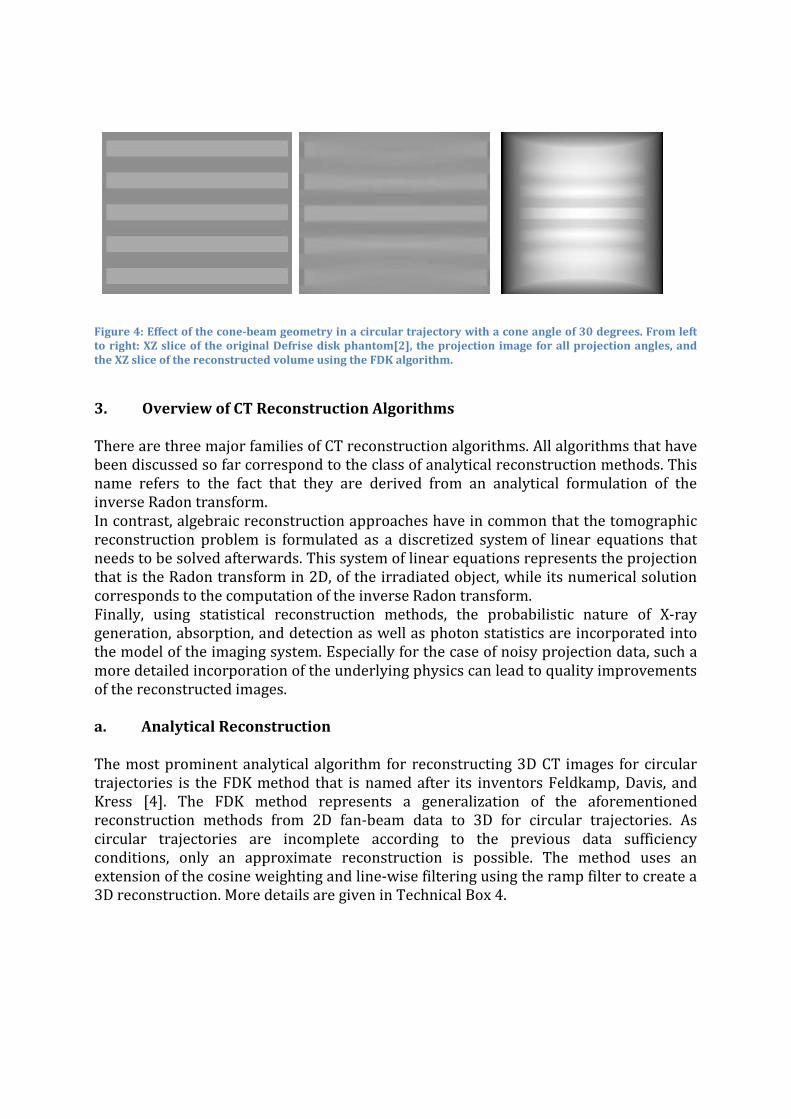
Figure 4: Effect of the cone-beam geometry in a circular trajectory with a cone angle of 30 degrees. From left to right: XZ slice of the original Defrise disk phantom[2], the projection image for all projection angles, and the XZ slice of the reconstructed volume using the FDK algorithm.

3. Overview of CT Reconstruction Algorithms

There are three major families of CT reconstruction algorithms. All algorithms that have been discussed so far correspond to the class of analytical reconstruction methods. This name refers to the fact that they are derived from an analytical formulation of the inverse Radon transform. In contrast, algebraic reconstruction approaches have in common that the tomographic reconstruction problem is formulated as a discretized system of linear equations that needs to be solved afterwards. This system of linear equations represents the projection that is the Radon transform in 2D, of the irradiated object, while its numerical solution corresponds to the computation of the inverse Radon transform. Finally, using statistical reconstruction methods, the probabilistic nature of X-ray generation, absorption, and detection as well as photon statistics are incorporated into the model of the imaging system. Especially for the case of noisy projection data, such a more detailed incorporation of the underlying physics can lead to quality improvements of the reconstructed images.

a. Analytical Reconstruction The most prominent analytical algorithm for reconstructing 3D CT images for circular trajectories is the FDK method that is named after its inventors Feldkamp, Davis, and Kress [4]. The FDK method represents a generalization of the aforementioned reconstruction methods from 2D fan-beam data to 3D for circular trajectories. As circular trajectories are incomplete according to the previous data sufficiency conditions, only an approximate reconstruction is possible. The method uses an extension of the cosine weighting and line-wise filtering using the ramp filter to create a 3D reconstruction. More details are given in Technical Box 4.

In contrast, Katsevich [5] proposed a general algorithmic framework for 3D CT reconstruction that leads to theoretically exact reconstruction results. Consequently, these Katsevich-type algorithms require X-ray source trajectory segments in addition to a circular trajectory such that projection data is captured completely according to Tuy’s sufficiency condition. It is important to point out that FDK-type approximate methods as well as Katsevich-type exact methods also exist for helical scan paths[2]. A more detailed description of the underlying theory is beyond the scope of this introduction to CT reconstruction methods. We refer to the corresponding literature [2]. b. Algebraic Reconstruction In the algebraic approaches, the object to be reconstructed is represented as an ensemble of discrete voxels (in 3D) or pixels (in 2D), and the irradiation process is considered as a sampling of the voxel- (or pixel-) dependent X-ray attenuation values along a discrete set of X-rays. Typically, there is one X-ray assigned to each detector value. This leads to a system 𝑨𝒙 = 𝒑 of linear equations that needs to be solved numerically [1]. Due to the size of the problem, computationally attractive and memory-efficient algorithms are commonly used. The column vector x denotes the unknown X-ray attenuation coefficients to be determined. The detector values, i.e., the line integrals of X-ray attenuation, are covered by the detector measurement vector p on the right-hand side, which is given as a column vector as well. In addition, the entries of the system matrix A are typically defined by the intersection lengths of the X-rays with the respective pixels (in 2D) or voxels (in 3D) or by some other interpolation scheme based on the use of more sophisticated basis functions (cf. [6]). Note that this reconstruction approach is completely independent of the CT acquisition geometry. All geometry information inherent to a specific CT scanner is contained in the elements of A. Thus, all algebraic solution schemes are independent of the scanner geometry and no specific conversions from one geometry to another have to be performed.

𝑓(𝑥,𝑦, 𝑧) =12� 2𝜋

0

1𝑈′2

�𝐷

√𝐷2 + 𝑡2 + 𝑢2𝑔(𝑡,𝑢,𝛽) ⋅ ℎ(𝑡′ − 𝑡) d𝑡d𝛽.

∞

−∞

Technical Box 4: Feldkamp-Davis-Kress Reconstruction For the case of a flat-panel data 𝑔(𝑡,𝑢,𝛽), which is characterized by an array of equally sized detector pixels (𝑡,𝑢) and thus represents a 2D extension of a linear detector 𝑔(𝑡,𝛽), the FDK algorithm is based on the following approximation of the inversion formula:

Tuy’s sufficiency condition implies that the FDK method is only correct for special cases. In general, it delivers only approximate reconstruction results due to the incomplete set of projection data that results from a circular scan trajectory.

In the following figure, a simple example is shown. It is assumed that nine detector values are measured, which leads to an overall number of nine linear equations.

𝑥1 + 𝑥2 + 𝑥3 = 𝑝1 𝑥4 + 𝑥5 + 𝑥6 = 𝑝2 𝑥7 + 𝑥8 + 𝑥9 = 𝑝3 𝑥3 + 𝑥6 + 𝑥9 = 𝑝4 𝑥2 + 𝑥5 + 𝑥8 = 𝑝5 𝑥1 + 𝑥4 + 𝑥7 = 𝑝6

2(√2 − 1)𝑥4 + (2 − √2)𝑥4 + 2(√2 − 1)𝑥8 = 𝑝7 (√2)𝑥1 + (√2)𝑥5 + (√2)𝑥9 = 𝑝8

2(√2 − 1)𝑥2 + (2 − √2)𝑥3 + 2(√2 − 1)𝑥6 = 𝑝9 Figure 5: Representation of the CT reconstruction problem as a system of linear equations, which is an essential step when solving the reconstruction task algebraically.

𝒙𝒊 = 𝒙𝒊−𝟏 +𝑝𝑖 − 𝑨𝒊 𝒙𝒊𝑨𝒊 𝑨𝒊⊤

𝑨𝒊⊤,

Technical Box 5: Algebraic Reconstruction Technique (ART) The ART possesses an intuitive geometrical interpretation. Each of the linear equations represents a (hyper-) plane in the solution space. For example, for the very simple case of a reconstruction problem with two unknown pixels only, each equation defines a line in the 2D plane. The ART can be illustrated as a successive orthogonal projection of the respective approximate solution onto the (hyper-) planes defined by the individual linear equations. The orthogonal projection of the approximation 𝒙𝒊−𝟏 onto the (hyper-) plane defined by the i-th equation yields the approximation 𝒙𝒊 and is formally given by

where the row vector 𝑨𝒊 represents the i-th matrix row and 𝑝𝑖 denotes the i-th entry of the right-hand side vector p. The ART can therefore be formulated as a numerical iteration scheme that computes any approximation 𝒙𝒌+𝟏 from the previous approximation 𝒙𝒌 until some appropriate termination criterion for the iteration process is reached. A single ART iteration that computes 𝒙𝒌+𝟏 from 𝒙𝒌 reads as follows: 𝒙𝟎 = 𝒙𝒌 for 𝑖 = 1 to number of equations 𝑁 (= rows of A): 𝒙𝒊 = 𝒙𝒊−𝟏 + 𝑝𝑖−𝑨𝒊 𝒙𝒊−𝟏

𝑨𝒊 𝑨𝒊⊤ 𝑨𝒊⊤

end for 𝒙𝒌+𝟏 = 𝒙𝑵 A suitable termination criterion can for example be based on the relative change of one approximate solution to the next or on the length of the current reprojection error 𝒓𝒌 = 𝒑 − 𝑨𝒙𝒌 that measures how well 𝒙𝒌 fulfills the linear system 𝑨𝒙 = 𝒑.

𝑃�𝑋𝑗 = 𝑘; 𝑥𝑗� =1𝑘!𝑒

–𝑥𝑗𝑥𝑗 𝑘 ,

𝑃(𝑌𝑖 = 𝑦𝑖;𝒙) =1𝑦𝑖!

𝑒 –𝑦𝑖(𝒙)𝑦𝑖(𝒙)

𝑦𝑖 ,

𝐿(𝒙) = �𝑃(𝑌𝑖 = 𝑦𝑖;𝒙)𝑦𝑖

.

log 𝐿(𝒙) = log �𝑃(𝑌𝑖 = 𝑦𝑖;𝒙)𝑦𝑖

= �(𝑦𝑖 log 𝑦𝑗(𝒙) − (𝑦𝑗(𝒙) + 𝑟𝑖) + log (1𝑦𝑖!

)),𝑦𝑖

𝑑(𝒙|𝒀) =𝑑(𝒀|𝒙)𝑑(𝒙)

𝑑(𝒀)

log 𝑑(𝒙|𝒀) = log𝑑(𝒀|𝒙) + log𝑑(𝒙) = log 𝐿(𝒙) − 𝛽𝑅(𝒙).

Technical Box 6: Statistical Reconstruction In statistical reconstruction, the assumption is made that the absorption at a given voxel is a random variable 𝑋𝑗 that is distributed according to a Poission distribution with a mean value of 𝑥𝑗:

where 𝑘 is the actual absorption that occurred in the voxel. A ray passing through multiple voxels follows a Bernoulli process. In [7] it is shown that such a process leads to another Poisson-distributed random variable 𝑌𝑖:

where 𝑦𝑖 denotes the observed intensity at the detector and 𝑦𝑖(𝒙) denotes the accumulated absorption through the volume 𝒙 along the respective ray. Given that the observations at the detector are independent in 𝑦𝑖 the total probability for a given volume 𝒙 can be expressed using the likelihood function 𝐿(𝒙):

Since the application of a continuous rising function does not change the position of the maximum and all probabilities are non-negative, it is valid to take the logarithm on both sides to obtain the log likelihood function:

where 𝑟𝑖 are measurement errors that occur during the measurement process. This function can now be optimized to find the volume 𝒙 that fits the observations best in a maximum likelihood (ML) sense. In practice depending on the numerical method that was chosen for optimization different reconstruction algorithms emerge [8]. Note that log (1/(𝑦𝑖!)) is independent of 𝒙. Thus it is removed for the subsequent optimization process. Another approach towards solving the reconstruction problem is to consider the posterior distribution 𝑑(𝒙|𝒀) that can be expressed as

according to Bayes’ rule. For the sake of optimization, the logarithm is taken and 𝑑(𝒀) is removed as it is independent of 𝒙:

Note that log 𝐿(𝒙) is the previously defined log likelihood function. The term 𝑅(𝒙) emerges from prior knowledge 𝑑(𝒙) of 𝒙 and is commonly referred to as a regularization term. Using 𝑅(𝒙), additional properties such as smoothness or other constraints can be enforced in the optimization process. The weighting factor 𝛽 is used to control the influence of the regularization. As the posterior probability is maximized this kind of formulation is often referred to as maximum a-posteriori (MAP) estimation [2].

The different algebraic reconstruction methods result from the selected numerical algorithm that is applied in order to solve the previously generated linear system. For large reconstruction problems, i.e. reconstruction matrices, the linear system may not be assembled explicitly. In order to keep the memory footprint of the computer implementation as small as possible, it is rather generated on-the-fly. For example, consider a data set with 2563 voxels. The number of voxels corresponds to the number of unknowns. With 256 projections with 2562 pixels each, we have 2563 measurements; i.e., equations. This results in a system matrix 𝑨 ∈ ℝ2563×2563. In double precision floating-point arithmetic with 8 Bytes per matrix entry, this leads to a memory requirement of 2048 TB. The ART (Algebraic Reconstruction Technique), for instance, represents an elementary algebraic method. It is based on Kaczmarz’ projection scheme for solving systems of linear equations. As an iterative numerical algorithm, it aims at improving the current approximate solution from iteration to iteration. Technical Box 5 gives a short introduction into ART. The analysis of the convergence behavior of the ART as well as a discussion of more sophisticated numerical algorithms for the solution of large systems of linear equations such as Krylov subspace methods or multigrid schemes is beyond the scope of this overview and the reader is referred to the literature [1]. c. Statistical Reconstruction For the statistical reconstruction, the stochastic nature of the transmission process is taken into account. A short introduction into the idea is given in Technical Box 6. As it is the case for the family of algebraic reconstruction methods, different numerical solution approaches can be applied henceforth to solve the mathematical problem of parameter estimation; e.g., the expectation maximization (EM) method or different gradient descent methods [7]. A more comprehensive discussion of this large family of statistical CT reconstruction algorithms is again beyond the scope of this basic overview. We refer to [6] and [8] for details. 4. Practical Considerations In the previous sections, we discussed the fundamental methods that are required to reconstruct volumetric data. In practice, these methods are often altered to enable larger fields-of-view or to improve image quality. a. Toggle Mode The so-called toggle mode (or shuttle mode) is a technique for CT scanners to increase the size of the imaged field-of-view, i.e. the coverage in head-feet direction. The method is only applicable, if a certain slab of a volume needs to be scanned repeatedly, as it is the case for cardiac and brain perfusion CT [9]. In a conventional perfusion scan, only the volume that is covered by the source and the detector rotation is acquired while the patient remains stationary on the table. For a

reasonably accurate perfusion image, the patient should be repeatedly imaged at a frequency of about 1 Hz. CT gantries, however, can rotate at a much higher speed at a frequency of about 3 Hz. This fast rotation speed can therefore be exploited to increase the imaged field-of-view while maintaining a reasonable temporal sampling rate of the patient. The patient table is moved back and forth and the imaged volume is therefore increased in axial direction. b. Noise and Artifact Reduction As previously described, missing data on a circular trajectory creates a typical cone-beam artifact when reconstruction with an approximate algorithm is performed. Such artifact can be suppressed by extended reconstruction methods as proposed in [10]. A more detailed analysis of such methods is given in [11]. Many FBP reconstruction methods are derived in a continuous domain. The data, however, is acquired in a discrete manner. This discrepancy is often neglected, but may lead to major reconstruction artifacts, if it is not handled with caution [1]. As filtering is applied in many reconstruction algorithms, a truncation of the view in the filtering direction introduces high frequencies that corrupt the resulting reconstruction. This problem is usually corrected by an extrapolation step that is applied before [12] or during the filtering [13]. Another source of artifact emerges from under-sampled data. In this case, reconstruction is performed using only few projections or limiting the angular range. While reconstruction can still be performed correctly, if at least 180° [14] or more [15] are acquired for each point of the reconstructed object, reconstruction from less data suffers from limited angle-artifact. In general, most reconstruction algorithms do not model noise, beam-hardening, scatter, and photon starvation explicitly. They are often compensated in processing steps that are handled before or after the reconstruction [16][6][17][18] and are basically independent of the reconstruction method. c. C-arm CT Reconstruction as a Special Case For most CT scanners, the acquisition geometry is identical to the ideal geometry as they are built for this purpose. However, there are devices that do not fulfill this requirement, but are still able to reconstruct cone-beam CT data. Rotational angiography systems for instance, deviate considerably from the ideal trajectory. The geometry of these machines can be calibrated using standard camera calibration methods [19]. Therefore, a phantom of known geometric properties is scanned and the projection geometry is computed from markers of known location on the phantom [20][19]. Furthermore, the slow rotation speed of these systems is a challenge for the image reconstruction, if the object is not static, as it is assumed in most reconstruction algorithms. In order to cope with these effects, either repeated scans with different synchronization strategies [21] are applied or the effect of motion is modeled explicitly [22][23][24]. 5. New Directions

CT reconstruction is a vivid field of research, and it is impossible to name all of the new directions that are being investigated at present. Therefore, we will only give a short description of recent advances in current research in the opinion of the authors. Hardware accelerated reconstruction: With the availability of low-cost high performance hardware such as fast graphics boards computationally infeasible reconstruction approaches like iterative methods are reconsidered again [25]. Iterative methods exhibit the advantage that they can be regularized towards a certain solution [26]. This may also include the use of prior knowledge [27] such as atlas data or preceding reconstruction results. Motion compensated reconstruction: In present CT theory, the reconstructed object is assumed to be static. This may, however, not be the case in all applications [21]. In order to mend the problem of motion in the acquired data, a motion field can be estimated. In this way, we can differentiate the motion of the object from the rotating motion during the acquisition and perform a motion compensated reconstruction [24]. While this approach can be applied to many scenarios, the main challenge is to estimate the motion correctly [23]. Benchmark data sets: Another interesting trend for the scientific evaluation of reconstruction methods is to share a common problem with the scientific community and to publish a list with the best known results. In the context of the RabbitCT project [28], for example, a comparison of fast reconstruction methods is found. CAVAREV [22] focuses on the accuracy of the reconstruction of the cardiac vasculature. Reconstruction from sparse data: Many acquisition scenarios do provide projections from limited angles or only sparse set of projection images. In tomosynthesis [29], which is particularly used in mammography, limited angle reconstruction is a rather demanding issue. The reconstruction of high contrast objects from sparse projections is considered in discrete tomography [30] as well as in the context of compressed sensing approaches [27][31]. Spectral reconstruction: Modern CT scanners and their reconstruction algorithms rely on the assumption that monochromatic X-ray is used for image acquisition. If detectors are able to measure the spectrum of X-ray, reconstruction algorithms will be required to perform spectral reconstruction, that is reconstruction of engery-dependent absorption coefficients. The development of this new generation of reconstruction algorithms is part of intense research [32]. Phase Contrast CT: As X-rays propagate through material their attenuation and phase is altered. In conventional X-ray imaging only the attenuation is used. Both attenuation and phase shift, however, depend on material properties. Thus both contain useable information. In phase contrast CT, the phase shift is measured and the reconstruction is done on the basis of these measurements [33]. Additional diagnostic value is presently under investigation.

Bibliography [1] Kak AC, Slaney M, Principles of Computerized Tomographic Imaging. Piscataway, NJ,

United States: IEEE Service Center, 1988. [2] Zeng L, Medical Image Reconstruction: A Conceptual Tutorial. Heidelberg Dordrecht

London New York, United States of America: Springer, 2009. [3] Hein I, Taguchi K, Mori I, Kazama M, Silver M, "Tilted helical Feldkamp cone-beam

reconstruction algorithm for multislice CT," in Proc SPIE Medical Imaging, San Diego, California, USA, 2003.

[4] Feldkamp LA, Davis LC, Kress JW, "Practical cone beam algorithm," Journal of the Optical Society of America, vol. 1, pp. 612-619, 1984.

[5] Katsevich A, "Theoretically exact filtered backprojection-type inversion algorithm for spiral CT," SIAM Journal of Applied Mathematics, vol. 62, no. 6, pp. 2012-2026, 2002.

[6] Buzug T, Computed Tomography - From Photon Statistics to Modern Cone-Beam CT. Berlin, Germany: Springer, 2008.

[7] Fessler A, "Statistical Image Reconstruction Methods," in Handbook of Medical Imaging, Volume 2. Medical Image Processing and Analysis, Sonka M Fitzpatrick M, Ed. Bellingham, Washington USA: SPIE Press, 2000, ch. 1, pp. 1-70.

[8] Lange K, Fessler JA, "Globally Convergent Algorithms for a Maximum a Posteriori Transmission Tomography," IEEE Transactions on Image Processing, vol. 4, no. 10, pp. 1430-1438, 1995.

[9] Fieselmann A, Kowarschik M, Ganguly A, Hornegger J, Fahrig R, "Deconvolution-Based CT and MR Brain Perfusion Measurement: Theoretical Model Revisited and Practical Implementation Details," Journal of Biomedical Imaging, 2011, Article ID 467563, 20 pages.

[10] Dennerlein F, Noo F, Lauritsch G, Hornegger J, "A Factorization Approach for Cone-beam Reconstruction on a Circular Short-Scan," IEEE Transactions on Medical Imaging, vol. 27, no. 7, pp. 887-896, 2008.

[11] Dennerlein F, Image Reconstruction from Fan-Beam and Cone-Beam Projections. Erlangen, Germany: Dissertation, Universität Erlangen-Nürnberg, 2008.

[12] Ohnesorge B, Flohr T, Schwarz K, Heiken JP, Bae KT, "Efficient correction for CT image artifacts caused by objects extending outside the scan field of view.," Medical Physics, vol. 27, no. 1, pp. 39-46, 2000.

[13] Dennerlein F, Maier A, "Region-Of-Interest Reconstruction on medical C-arms with the ATRACT Algorithm," in Proceedings SPIE 8313, San Diego, California, USA, 2012, p. 83131B.

[14] Noo F, Defrise M, Clackdoyle R, Kudo H, "Image reconstruction from fan-beam projections on less than a short scan," Physics in Medicine and Biology, vol. 47, no. 14, pp. 2525-2546, 2002.

[15] Parker DL, "Optimal short scan convolution reconstruction for fanbeam CT," Medical Physics, vol. 9, no. 2, pp. 254-257, 1982.

[16] Maier A, Wigström L, Hofmann HG, Hornegger J, Zhu L, Strobel N, Fahrig R, "Three-dimensional Anisotropic Adaptive Filter-ing of Projection Data for Noise Reduction in Cone Beam CT," Medical Physics, vol. 38, no. 11, pp. 5896-5909, 2011.

[17] Zellerhoff M, Scholz B, Rührnschopf EP, Brunner T, "Low contrast 3-D reconstruction from C-arm data," in Proceedings of the SPIE, Volume 5745, San Diego, United States, 2005, pp. 646-55.

[18] Perona P, Malik J, "Scale space and edge detection using anisotropic diffusion," IEEE Transactions on Pattern Analysis and Machine Intelligence, vol. 12, pp. 629-39, 1990.

[19] Maier A, Choi JH, Keil A, Niebler C, Sarmiento M, Fieselmann A, Gold G, Delp S, Fahrig R, "Analysis of Vertical and Horizontal Circular C-Arm Trajectories," in Proceedings SPIE 7961, Lake Buena Vista, Florida, USA, 2011, p. 796123.

[20] Hoppe S, Accurate Cone-Beam Image Reconstruction in C-Arm Computed Tomography. Erlangen, Germany: Dissertation, Universität Erlangen-Nürnberg, 2008.

[21] Lauritsch G, Boese J, Wigström L, Kemeth H, Fahrig R, "Towards cardiac C-arm computed tomography," IEEE Transactions on Medical Imaging, vol. 25, pp. 922-34, 2006.

[22] Rohkohl C, Lauritsch G, Keil A, Hornegger J, "CAVAREV—an open platform for evaluating 3D and 4D cardiac vasculature reconstruction," Physics in Medicine and Biology, vol. 55, pp. 2905-2915, 2010.

[23] Rohkohl C, Motion Estimation and Compensation for Interventional Cardiovascular Image Reconstruction. Erlangen, Germany: Dissertation, Universität Erlangen-Nürnberg, 2011.

[24] Prümmer M, Cardiac C-Arm Computed Tomography: Motion Estimation and Dynamic Reconstruction. Erlangen, Germany: Dissertation, Universität Erlangen-Nürnberg, 2009.

[25] Scherl H, Kowarschik M, Hofmann HG, Keck B, Hornegger J, "Evaluation of state-of-the-art hardware architectures for fast cone-beam CT reconstruction," Parallel Computing, vol. 38, pp. 111-124, 2012.

[26] Sidky EY, Pan X, "Image reconstruction in circular cone-beam computed tomography by constrained, total-variation minimization," Physics in Medicine and Biology, vol. 53, no. 17, pp. 4777-4807, 2008.

[27] Chen GH, Tang J, Leng S, "Prior image constrained compressed sensing (PICCS): A method to accurately reconstruct dynamic CT images from highly undersampled projection data sets," Medical Physics, vol. 35, no. 2, pp. 660-663, 2008.

[28] Rohkohl C, Keck B, Hofmann H, Hornegger J, "RabbitCT - an open platform for benchmarking 3D cone-beam reconstruction algorithms," Medical Physics, vol. 36, no. 9, pp. 3940-3944, 2009.

[29] Dobbins JT, Godfrey DJ, "Digital x-ray tomosynthesis: current state of the art and clinical potential," Physics in Medicine and Biology, vol. 48, no. 19, pp. R65-R106, 2003.

[30] Kuba A, Herman GT, Ed., Advances in Discrete Tomography and Its Applications, Applied and Numerical Harmonic Analysis. Boston, USA: Birkhäuser, 2007.

[31] Wu H, Maier A, Hofmann H, Fahrig R, Hornegger J, "4D-CT Reconstrucion Using Sparsity Level Constrained Compressed Sensing," in 2nd CT Meeting, Salt Lake City, 2012, pp. 206-209.

[32] Heismann B, Balda M, "Quantitative image-based spectral reconstruction for computed tomography," Medical Physics, vol. 36, no. 10, pp. 4471-4485, 2009.

[33] Pfeiffer F, Weitkamp T, Bunk O, David C, "Phase retrieval and differential phase-contrast imaging with low-brilliance X-ray sources," Nature Physics , no. 2, pp. 258 - 261 , 2006.

[34] Apostol T, Mathematical Analysis, 2nd ed.: Addison Wesley, 1974.