ctdas-lagrange v1.0: a high-resolution data assimilation

Geosci. Model Dev., 11, 3515–3536, 2018https://doi.org/10.5194/gmd-11-3515-2018© Author(s) 2018. This work is distributed underthe Creative Commons Attribution 4.0 License.

CTDAS-Lagrange v1.0: a high-resolution data assimilation systemfor regional carbon dioxide observationsWei He1,2, Ivar R. van der Velde3,4, Arlyn E. Andrews3, Colm Sweeney3,4, John Miller3, Pieter Tans3,Ingrid T. van der Laan-Luijkx5, Thomas Nehrkorn6, Marikate Mountain6, Weimin Ju1, Wouter Peters2,5, andHuilin Chen2,4

1International Institute for Earth System Science, Nanjing University, Nanjing, China2Center for Isotope Research (CIO), Energy and Sustainability Research Institute Groningen (ESRIG),University of Groningen, Groningen, 9747 AG, the Netherlands3Global Monitoring Division, NOAA Earth System Research Laboratory, Boulder, Colorado, USA4Cooperative Institute for Research in Environmental Sciences (CIRES), University of Colorado, Boulder, Colorado, USA5Department of Meteorology and Air Quality, Wageningen University, Wageningen, the Netherlands6Atmospheric and Environmental Research, Lexington, MA, USA

Correspondence: Huilin Chen ([email protected])

Received: 7 September 2017 – Discussion started: 5 December 2017Revised: 25 May 2018 – Accepted: 15 August 2018 – Published: 30 August 2018

Abstract. We have implemented a regional carbon diox-ide data assimilation system based on the CarbonTrackerData Assimilation Shell (CTDAS) and a high-resolution La-grangian transport model, the Stochastic Time-Inverted La-grangian Transport model driven by the Weather Forecastand Research meteorological fields (WRF-STILT). With thissystem, named CTDAS-Lagrange, we simultaneously opti-mize terrestrial biosphere fluxes and four parameters that ad-just the lateral boundary conditions (BCs) against CO2 obser-vations from the NOAA ESRL North America tall tower andaircraft programmable flask packages (PFPs) sampling pro-gram. Least-squares optimization is performed with a time-stepping ensemble Kalman smoother, over a time windowof 10 days and assimilating sequentially a time series ofobservations. Because the WRF-STILT footprints are pre-computed, it is computationally efficient to run the CTDAS-Lagrange system.

To estimate the uncertainties in the optimized fluxesfrom the system, we performed sensitivity tests with vari-ous a priori biosphere fluxes (SiBCASA, SiB3, CT2013B)and BCs (optimized mole fraction fields from CT2013B andCTE2014, and an empirical dataset derived from aircraft ob-servations), as well as with a variety of choices on the waysthat fluxes are adjusted (additive or multiplicative), covari-ance length scales, biosphere flux covariances, BC param-

eter uncertainties, and model–data mismatches. In pseudo-data experiments, we show that in our implementation theadditive flux adjustment method is more flexible in optimiz-ing net ecosystem exchange (NEE) than the multiplicativeflux adjustment method, and our sensitivity tests with realobservations show that the CTDAS-Lagrange system has theability to correct for the potential biases in the lateral BCsand to resolve large biases in the prior biosphere fluxes.

Using real observations, we have derived a range of esti-mates for the optimized carbon fluxes from a series of sensi-tivity tests, which places the North American carbon sink forthe year 2010 in a range from−0.92 to−1.26 PgC yr−1. Thisis comparable to the TM5-based estimates of CarbonTracker(version CT2016, −0.91± 1.10 PgC yr−1) and Carbon-Tracker Europe (version CTE2016, −0.91±0.31 PgC yr−1).We conclude that CTDAS-Lagrange can offer a versatile andcomputationally attractive alternative to these global systemsfor regional estimates of carbon fluxes, which can take ad-vantage of high-resolution Lagrangian footprints that are in-creasingly easy to obtain.

Published by Copernicus Publications on behalf of the European Geosciences Union.

3516 W. He et al.: CTDAS-Lagrange v1.0

1 Introduction

CO2 exchange between the terrestrial biosphere and theatmosphere has a strong impact on the climate system(Houghton et al., 2001), which makes it crucial to quan-tify the amount of CO2 exchange, and to better understandthe interactions between the global carbon cycle and climatechange. Atmospheric measurements of trace gas mole frac-tions provide constraints for the estimates of biosphere sur-face fluxes from regional to global scales (Schuh et al., 2010;Lauvaux et al., 2012; Peters et al., 2007; Peylin et al., 2013;van der Laan-Luijkx et al., 2017), and complement bottom-up biosphere modeling (Sellers et al., 1996; Schaefer et al.,2008; van der Velde et al., 2014) that typically targets siteto ecosystem scales in the earth system. Inferring biosphericand oceanic surface fluxes from a “top-down” perspective,through an atmospheric inversion, plays an important role inglobal budgeting efforts (Le Quéré et al., 2016), as it takesadvantage of the mass conservation of carbon in the atmo-sphere for global inversions and the high-precision measure-ments done in the atmosphere over the past decades (Con-way et al., 1994; observations are now published throughObsPack available at https://www.esrl.noaa.gov/gmd/ccgg/obspack/index.html, last access: 25 August 2018).

In the past decade, much attention has been given to esti-mating carbon fluxes at global scales (e.g., Rödenbeck et al.,2003; Peters et al., 2007; Chevallier et al., 2010; Peylin etal., 2013), while regional inversion studies with high spatialresolution for carbon fluxes are only gaining ground morerecently (e.g., Rödenbeck et al., 2019; Göckede et al., 2010;Schuh et al., 2010; Tolk et al., 2011; Lauvaux et al., 2012;Gourdji et al., 2012; Broquet et al., 2013; Shiga et al., 2014;Alden et al., 2016; Kountouris et al., 2018). Such regionalinversion studies contribute to a better understanding of themechanism through which carbon fluxes react to environ-mental variations at a fine scale. But to link carbon fluxes andenvironmental drivers to atmospheric measurements, a high-resolution transport model is typically needed. In the frame-work for global inversions, typically, ensemble-based meth-ods (Peters et al., 2007) are based on Eulerian models, andanalytical methods (Rödenbeck et al., 2003; Chevallier et al.,2010) are with a linearized adjoint model of such Eulerianmodels. In terms of computational efficiency, Lagrangianmodels are superior to these traditional Eulerian models forhigh-resolution applications, which makes them suitable forcomputation-intensive regional atmospheric inversions. Thecomputation cost of Lagrangian models increases with theincreasing number of observations; however, it remains anadvantage that offline Lagrangian transport results, i.e., foot-prints need to be computed only once, can be stored for futureuse.

However, both global and regional inversion studies suf-fer from various uncertainties, including transport and rep-resentation errors, possible observational biases when datafrom different laboratories are combined, and uncertainties

in a priori fluxes. For regional inversions, errors in lateralboundary conditions (BCs) become another critical issue(Alden et al., 2016; Gerbig et al., 2003; Schuh et al., 2010;Lauvaux et al., 2013), and can bias flux estimates, particu-larly for smaller areas (Göckede et al., 2010) and for shorterperiods (Andersson et al., 2015). Several methods to createlateral BCs have been employed, including deriving themfrom mole fraction fields of global inversions (Kountouris etal., 2018) and in situ mole fraction observations, e.g., air-craft profiles or satellite observations (Jiang et al., 2015).Embedding a regional inversion inside a global model do-main has been widely applied for CO2, CH4, and N2O fluxestimates (Bergamaschi et al., 2010; Corazza et al., 2011), forexample within the nested TM5 model framework. Gourdjiet al. (2012) compared an empirical BC derived from aircraftprofiles and marine boundary layer data with BC values takenfrom CarbonTracker CT2009 optimized mole fraction fields,and pointed out the former might be more accurate than thelatter. Various studies apply aircraft measurements to correctmodel-derived BCs either before (Broquet et al., 2013) orduring regional inversions (Lauvaux et al., 2012; Brioude etal., 2013; Wecht et al., 2014). Adjusting BCs using the in-verse modeling framework is desirable as it guarantees con-sistency between all sources of information used. Recently,Jiang et al. (2015) assimilated the MOPITT satellite profiledata to optimize BCs during the estimation of North Amer-ican CO emissions, and reported a reduction of the meanresidual bias in the posteriori simulation (simulations minusobservations) from −13.3 % to 3.5 %.

To better understand regional carbon fluxes, we developeda data assimilation system that employs a high-resolutionLagrangian atmospheric transport model, the WRF-STILTmodel. Our assimilation system, the CarbonTracker DataAssimilation Shell – Lagrange, (referred to as “CTDAS-Lagrange”), is based on the CarbonTracker Europe system,which is a widely applied global inversion system (Peterset al., 2010; van der Laan-Luijkx et al., 2015, 2017). Inour new system, we optimize BCs using independent in-formation from aircraft profiles. We use a priori biospherefluxes from the SiBCASA biosphere model (Schaefer etal., 2008), and the other a priori fluxes for the componentsocean, fossil fuels, and fires are from CT2013B (accessiblefrom the archived release https://www.esrl.noaa.gov/gmd/ccgg/carbontracker/CT2013B/, last access: 25 August 2018).CO2 observations come from the NOAA programmable flaskpackage (PFP) data from tall towers and aircraft sites. Air-craft observations are used to optimize BCs while tower ob-servations were used to optimize the terrestrial biospherefluxes at the surface. We investigate the impact of differenta priori fluxes and BCs, two alternative ways of adjustingfluxes (additive and multiplicative), covariance length scales,BC parameter uncertainties, model–data mismatch, and un-certainties from transport on the optimized fluxes. Based onthe above investigations, we have constructed a range of esti-

Geosci. Model Dev., 11, 3515–3536, 2018 www.geosci-model-dev.net/11/3515/2018/

https://www.esrl.noaa.gov/gmd/ccgg/obspack/index.html

https://www.esrl.noaa.gov/gmd/ccgg/obspack/index.html

https://www.esrl.noaa.gov/gmd/ccgg/carbontracker/CT2013B/

https://www.esrl.noaa.gov/gmd/ccgg/carbontracker/CT2013B/

W. He et al.: CTDAS-Lagrange v1.0 3517

mates, and then compared the inversion results with those ofcontemporary inversion studies.

The purpose of this paper is to describe and demonstratethe CTDAS-Lagrange data assimilation system. We have per-formed preliminary inversions using a subset of the avail-able CO2 data for North America for a single year. A morecomprehensive analysis is planned that will incorporate ad-ditional datasets and cover a longer time period. This paperis organized as follows: in Sect. 2 we introduce the modelingframework and observation data used for this study, Sect. 3presents results of the system performance and sensitivityruns, followed by discussion and conclusions in Sect. 4.

2 Data and model

2.1 CO2 observations

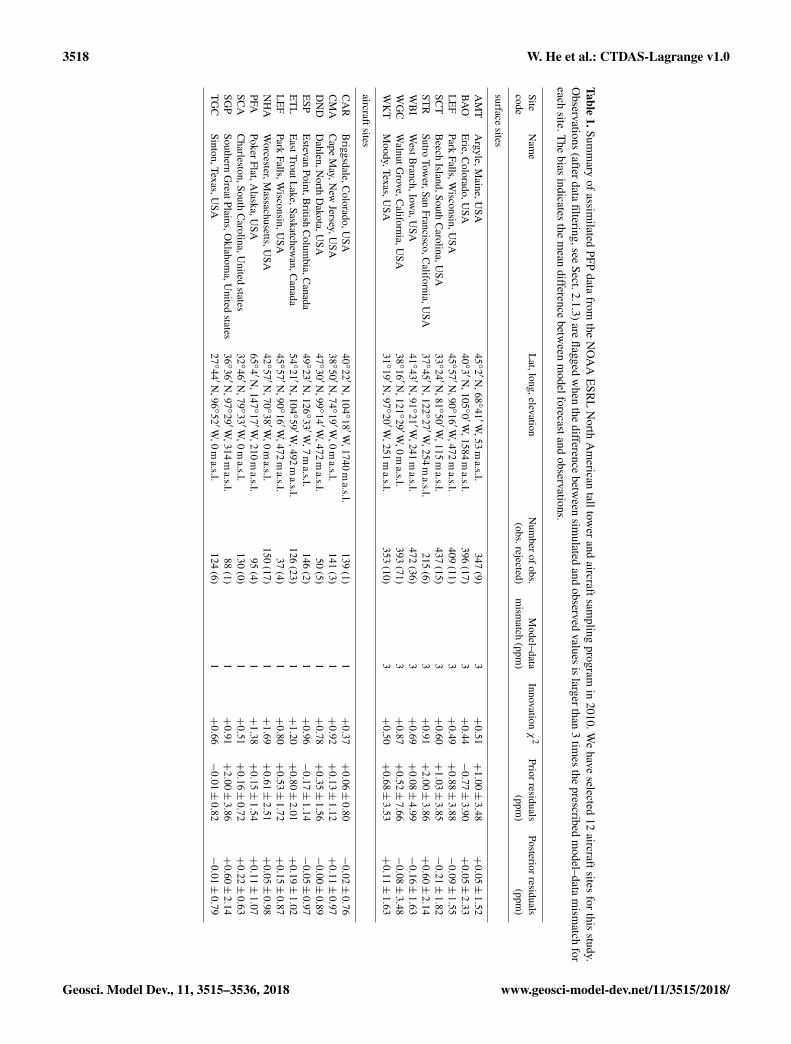
Our system assimilates atmospheric CO2 mole fraction mea-surements made from the NOAA ESRL Global GreenhouseGas Reference Network, specifically the analysis results ofair samples collected by automated flask-sampling systemsthat are known as programmable flask packages (PFPs). Theadvantage of using PFP flask data is that more than 50compounds, including carbon monoxide, are also availabletogether with CO2 measurements. These data collected inNorth America at 8 tall tower sites and 12 selected aircraftsites in 2010 are used for this study. The air samples werecollected daily or on alternate days during mid-afternoon atthe tall tower sites (Andrews et al., 2014), and biweekly ormonthly at the selected aircraft sites (Sweeney et al., 2015).The location of the observations is shown in Fig. 1. The dataare provided to the model input as an ObsPack (Masarie etal., 2014).

2.1.1 Tall tower observations

Detailed site and sampling information of the tall tower ob-servations is listed in Table 1. Andrews et al. (2014) usedflask versus in situ comparisons for quality control andpointed out such comparisons suffer from quasi-continuousin situ data (due to, for example, switching of sampling linesamong different heights, calibrations), difference in samplingtime, and atmospheric variability. The mean differences be-tween PFP and in situ CO2 measurements over all eight sitesfor 2010 range from 0.08 to 0.32 ppm, with the standard de-viation of the differences for each site ranging from 0.2 to0.6 ppm and increasingly positive differences over the period2008–2011. According to Andrews et al. (2014), the meandifferences are likely caused by potential biases in an increas-ing number of the PFP measurements that may result fromcontamination caused by routine use throughout the networkor by use under polluted conditions. A new flask samplingprotocol was implemented in September such that the flaskis pressurized with ambient air prior to sample collection andheld at high pressure for several minutes then vented and re-

sampled. Agreement has improved between flask and in situmeasurement systems so the difference is reliably better than0.2 ppm. We did not make any attempt to correct for the po-tential biases in the 2010 data. Masarie et al. (2011) showsthat every 1 ppm of bias at Park Falls, Wisconsin, (labeledLEF) in the CarbonTracker inversion causes a linear responserate of 68 Tg C yr−1 for temperate North American net fluxestimates. However, if the bias is across the whole network,the impact on the net flux estimates will be much less thanthat.

2.1.2 Aircraft profiles

The NOAA ESRL aircraft CO2 profile data (Table 1) are usedto optimize lateral BCs. The aircraft program of the GlobalGreenhouse Gas Reference Network (Sweeney et al., 2015)has been collecting air samples for vertical profile measure-ments over North America since 1992. For each individ-ual flight, 12 flask samples are collected from 500 m aboveground up to 8000 m above sea level at most aircraft sites.Of the 15 ongoing aircraft sites by 2014, we have selected12 sites (8 close to the domain boundary, and 4 in the middleof the domain) for this study. Because the aircraft programuses the same PFP flasks as in the tall tower program, the air-craft CO2 measurements may have potential biases as well.Indeed, Karion et al. (2013) reported PFP minus in situ CO2measurements of 0.20± 0.37 ppm for the aircraft measure-ments over Alaska from 2009 to 2011, a similar magnitudeof biases as found in the tall tower PFP versus in situ com-parisons.

2.1.3 Data filtering

We use daytime data from the tall towers that are collectedbetween 10:00 and 18:00 local time to constrain surfacefluxes. Aircraft observations made at altitudes higher than3000 m above ground at all hours are used to constrain BCs.In CTDAS-Lagrange, we use fossil fuel emissions based oninventory estimates and do not attempt to optimize them. Weremove CO2 observations that are likely strongly influencedby fossil fuels before optimizing biosphere fluxes. This di-minishes the potential biases in optimized biosphere fluxesthat are caused by local fossil fuel sources and/or by rep-resentation errors in the simulated fossil fuel CO2 signals.To achieve this, we use CO measurements as a proxy forfossil fuel influences, realizing that especially in summerother sources of CO can contribute to enhanced mole frac-tions. We first calculate CO enhancement as the differencebetween the CO observation and the background value, i.e.,the corresponding value from a second order harmonic func-tion that is fitted to the CO data for each tall tower site.We filter out any CO2 observations with CO enhancementslarger than 33.6 ppb, which corresponds to 3 ppm fossil fuelCO2 according to the year-round median apparent ratio of11.2 ppb ppm−1, estimated in Miller et al. (2012). About

www.geosci-model-dev.net/11/3515/2018/ Geosci. Model Dev., 11, 3515–3536, 2018


Table1.Sum

mary

ofassim

ilatedPFP

datafrom

theN

OA

AE

SRL

North

Am

ericantalltow

erand

aircraftsampling

programin

2010.We

haveselected

12aircraftsites

forthis

study.O

bservations(afterdata

filtering,seeSect.2.1.3)are

flaggedw

henthe

differencebetw

eensim

ulatedand

observedvalues

islargerthan

3tim

esthe

prescribedm

odel–datam

ismatch

foreach

site.The

biasindicates

them

eandifference

between

modelforecastand

observations.

SiteN

ame

Lat,long,elevation

Num

berofobs.M

odel–dataInnovation

χ2

PriorresidualsPosteriorresiduals

code(obs.rejected)

mism

atch(ppm

)(ppm

)(ppm

)

surfacesites

AM

TA

rgyle,Maine,U

SA45◦2′N

,68◦41′W

,53m

a.s.l.347

(9)3

+0.51

+1.00±

3.48

+0.05±

1.52

BA

OE

rie,Colorado,U

SA40◦3′N

,105◦0′W

,1584m

a.s.l.396

(17)3

+0.44

−0.77±

3.90

+0.05±

2.33

LE

FPark

Falls,Wisconsin,U

SA45◦57′N

,90◦16′W

,472m

a.s.l.409

(11)3

+0.49

+0.88±

3.88

−0.09±

1.55

SCT

Beech

Island,SouthC

arolina,USA

33◦24′N

,81◦50′W

,115m

a.s.l.437

(15)3

+0.60

+1.03±

3.85

−0.21±

1.82

STR

SutroTow

er,SanFrancisco,C

alifornia,USA

37◦45′N

,122◦27′W

,254m

a.s.l.215

(6)3

+0.91

+2.00±

3.86

+0.60±

2.14

WB

IW

estBranch,Iow

a,USA

41◦43′N

,91◦21′W

,241m

a.s.l.472

(36)3

+0.69

+0.08±

4.99

−0.16±

1.63

WG

CW

alnutGrove,C

alifornia,USA

38◦16′N

,121◦29′W

,0m

a.s.l.393

(71)3

+0.87

+0.52±

7.66

−0.08±

3.48

WK

TM

oody,Texas,USA

31◦19′N

,97◦20′W

,251m

a.s.l.353

(10)3

+0.50

+0.68±

3.53

+0.11±

1.63

aircraftsites

CA

RB

riggsdale,Colorado,U

SA40◦22′N

,104◦18′W

,1740m

a.s.l.139

(1)1

+0.37

+0.06±

0.80

−0.02±

0.76

CM

AC

apeM

ay,New

Jersey,USA

38◦50′N

,74◦19′W

,0m

a.s.l.141

(3)1

+0.92

+0.13±

1.12

+0.11±

0.97

DN

DD

ahlen,North

Dakota,U

SA47◦30′N

,99◦14′W

,472m

a.s.l.50

(5)1

+0.78

+0.35±

1.56

−0.00±

0.89

ESP

Estevan

Point,British

Colum

bia,Canada

49◦23′N

,126◦33′W

,7m

a.s.l.146

(2)1

+0.96

−0.17±

1.14

−0.05±

0.97

ET

LE

astTroutLake,Saskatchew

an,Canada

54◦21′N

,104◦59′W

,492m

a.s.l.126

(23)1

+1.20

+0.80±

2.01

+0.19±

1.02

LE

FPark

Falls,Wisconsin,U

SA45◦57′N

,90◦16′W

,472m

a.s.l.37

(4)1

+0.80

+0.53±

1.72

+0.15±

0.87

NH

AW

orcester,Massachusetts,U

SA42◦57′N

,70◦38′W

,0m

a.s.l.150

(17)1

+1.69

+0.61±

2.51

+0.05±

0.98

PFAPokerFlat,A

laska,USA

65◦4′N

,147◦17′W

,210m

a.s.l.95

(4)1

+1.38

+0.15±

1.54

+0.11±

1.07

SCA

Charleston,South

Carolina,U

nitedstates

32◦46′N

,79◦33′W

,0m

a.s.l.130

(0)1

+0.51

+0.16±

0.72

+0.22±

0.63

SGP

SouthernG

reatPlains,Oklahom

a,United

states36◦36′N

,97◦29′W

,314m

a.s.l.88

(1)1

+0.91

+2.00±

3.86

+0.60±

2.14

TG

CSinton,Texas,U

SA27◦44′N

,96◦52′W

,0m

a.s.l.124

(6)1

+0.66

−0.01±

0.82

−0.01±

0.79



Figure 1. The model domain is shown together with the CO2 observational sites from NOAA’s Global Greenhouse Gas Reference Networkand the aggregated Olson ecosystem types. Eight tall tower sites are highlighted by green triangles with black site code labels, and 12 selectedaircraft sites are highlighted by red dots with gray site code labels.

8.5 % of the available CO2 data is excluded by the CO filter,with the majority coming from the two sites in California,labeled STR and WGC.

2.2 The CTDAS-Lagrange system

The CTDAS-Lagrange system aims to improve the estimatesof regional carbon fluxes by combining a high spatial resolu-tion Lagrangian modeling framework with the existing Car-bonTracker Data Assimilation Shell (van der Laan-Luijkx etal., 2017). Transport of atmospheric CO2 in the main appli-cation of CTDAS, the CarbonTracker Europe system, is re-alized by using the global two-way nested transport modelTM5 (3◦× 2◦ global, and 1◦× 1◦ for one or more regionaldomains of interest) and driven by 3 h meteorological pa-rameters. The CTDAS-Lagrange system replaces the coarseTM5 transport model with a Lagrangian transport model withhigh spatial resolution. Another advantage of the CTDAS-Lagrange system is its significantly improved time efficiency.Outputs from the Lagrangian transport model can be storedas measurement footprints (influence functions) so that theCO2 mole fractions resulting from different surface flux con-figurations can be simulated offline afterwards, using simplematrix multiplications rather than full transport calculations.In addition, these stored outputs can be used for other speciesdirectly, significantly reducing the computation time whenperforming multiple or other species inversions, i.e., for theextension of our system to multi-species applications.

2.2.1 Atmospheric transport model

The Stochastic Time-Inverted Lagrangian Transport modelcoupled with the Weather Forecast and Research (WRF-STILT) is employed in our system (Lin et al., 2003; Nehrkornet al., 2010). The STILT model is a receptor-oriented frame-work that links surface fluxes of trace gases with atmosphericmole fractions. During a WRF-STILT run, an ensemble ofparticles is released at the observation location (receptor) ata certain time, and particles are transported backward drivenby the WRF wind fields. The influence function, i.e., foot-print, for that particular receptor and time can be computedbased on the density of the particles in the surface layer de-fined in STILT as the lower half of the well-mixed boundarylayer (Gerbig et al., 2003).

We leverage a footprint library created for the NOAA Car-bonTracker Lagrange regional inversion framework (https://www.esrl.noaa.gov/gmd/ccgg/carbontracker-lagrange/, lastaccess: 25 August 2018). The WRF-STILT model was runwith 500 particles that are traced backward for 10 days. TheWRF model (version 3.3.1 for the 2010 time period of thisstudy) was configured with a Lambert conformal map projec-tion to cover continental North America, with a spatial reso-lution of 10 km for the inner domain over the continental US(∼ 25–55◦ N; 135–65◦W) and 40 km for the outer domain(∼ 10–80◦ N; 170–50◦W), and 40 vertical layers, which issimilar to the configurations in Nehrkorn et al. (2010) andHu et al. (2015). The North American Regional Reanaly-sis (Mesinger et al., 2006) provided initial and lateral BCs.Model runs were initialized every 24 h, with the initial 6 hof each 30 h forecast discarded to allow for model spin-up.


https://www.esrl.noaa.gov/gmd/ccgg/carbontracker-lagrange/

https://www.esrl.noaa.gov/gmd/ccgg/carbontracker-lagrange/


Species-independent 10-day surface footprints with 1◦× 1◦

spatial resolution and hourly time resolution are computedwith STILT and stored for each measurement along withback-trajectories. Snapshots of the 3-dimensional particledistribution are also stored to enable assignment of boundaryvalues according to where particles intersect with the domainof the inversion.

2.2.2 Optimization scheme

In the CTDAS-Lagrange system, we extended the exist-ing ensemble Kalman smoother method as is implementedin CarbonTracker and CarbonTracker Europe (Peters et al.,2005, 2007, 2010; van der Laan-Luijkx et al., 2017) to si-multaneously optimize biosphere fluxes and BC parameters.

We use two alternative ways of adjusting the total surfacefluxes (additive and multiplicative), while simultaneously op-timizing the lateral BCs by optimizing four parameters thatare implemented as follows:

C (Xr, tr)= C0 (Xr, tr)+∑4

i=0Wi (Xr, tr) ·βi

+ S (Xr, tr|x,y, t) ·

f[λ, Fbio (x,y, t)

]Fff (x,y, t)

Focn (x,y, t)

Ffire (x,y, t)

, (1)

where C(Xr, tr) is the simulated CO2 mole fraction (ppm)at the location of the observation (receptor) Xr and time tr;C0(Xr, tr) refers to the contribution of advection from thelateral BC (ppm); βi (ppm) is adjusted to optimize the lat-eral BC for each of the four sides of the regional domain foreach 10-day period. The BC mole fraction βi is weightedby the pre-calculated coefficient Wi (Xr, tr) (unitless) thatis determined as the ratio of the number of particles ex-ited from one side of the domain to the number of parti-cles exited from all sides of the domain. The domain con-siders 3000 m as the top boundary, which means that the par-ticles that exited the domain below 3000 m, or did not leavethe domain within 10 days, were not used to calculate theweightWi (Xr, tr). In case all particles left the domain below3000 m, the weights of BC parameters were zero and the BCwas not adjusted. This choice reflects the dominant influenceof surface fluxes over lateral advection for particles that spentconsiderable time within the inner domains. S (Xr, tr|x,y, t)

is the footprint – sensitivity of mole fraction variationsto surface fluxes, ppm (µmol m−2 s−1)−1 – calculated withSTILT. Biosphere fluxes Fbio(x,y, t) (µmol m−2 s−1) are op-timized by either additively or multiplicatively optimizinga set of parameters λ (µmol m−2 s−1, or unitless) for each1× 1◦ grid in the domain for each 10-day period, repre-sented by the function f [λ,Fbio(x,y, t)] in the equation.Focn(x,y, t), Fff(x,y, t), and Ffire(x,y, t) denote the CO2fluxes (µmol m−2 s−1) exchanged with ocean, from fossil fu-els and fires, and these are fixed.

The state variables therefore include the gridded adjust-ing parameters for the biosphere fluxes (3078 land grids with1◦× 1◦ resolution over North America) plus those for thefour BC parameters, leading to a total of 3082 parameters foreach 10-day period. The state variables are optimized simul-taneously within each period. Considering that aircraft ob-servations above 3000 m mostly contain information aboutBCs and have low or even no sensitivity to surface fluxes, weoptimize the biosphere fluxes using tower observations only,and optimize BCs with both tower and aircraft observations.This separation is applied through localization of the Kalmangain matrix.

2.2.3 System setup

The system aims to optimize (non-fire) net ecosystem ex-change (NEE) of CO2 between biosphere and atmosphere,and requires prior biosphere fluxes, lateral BCs, and otherfixed fluxes such as fossil fuel emissions and ocean and firefluxes as model input. This section describes the setup of thebase case run.

We use biosphere fluxes simulated by the combined Sim-ple Biosphere and Carnegie-Ames-Stanford Approach (SiB-CASA) model (Schaefer et al., 2008) as a prior and fixed fos-sil fuel burning, ocean, and fire fluxes from CT2013B (Peterset al., 2007, with updates documented at http://carbontracker.noaa.gov, last access: 25 August 2018) with the latter two be-ing negligibly small in the annual mean over our domain ofinterest, but still included since they introduce spatiotempo-ral variations in CO2 mole fractions. More details about theseprior and the component fluxes are described in Sect. 2.2.4.The lateral BC is also taken from the 4-D mole fraction fieldssimulated by CT2013B. We use the WRF-STILT transportmodel. Here we give a short summary of the configuration ofthe base case run: we prescribe an additive biosphere fluxesuncertainty of 1.6 µmol m−2 s−1; a prior uncertainty in theBC parameters of 2.0 ppm, a model–data mismatch of 3 ppmfor surface sites and 1 ppm for aircraft sites, and a covariancelength scale of 750 km.

We estimate the additive flux adjustments for each gridbox in our domain, but a covariance structure is used toreduce the number of degrees of freedom in the state vec-tor, and to balance it with the number of available observa-tions. The covariance is calculated as an exponential func-tion that decreases with distance between grid boxes, us-ing a decorrelation length scale of 750 km. This covarianceis only used between grid boxes that have the same domi-nant plant-functional type, as specified though the ecoregionmaps that are also used in CT2013B. These in turn are basedon TransCom regions, as well as the Olson ecosystem clas-sification (Olson et al., 2002). Where CT2013B uses singlescaling factors for each ecoregion, our gridded approach hasapproximately 122 degrees of freedom within its 3078 addi-tive adjustment parameters as compared to an average of 112independent observations per assimilation time step.


http://carbontracker.noaa.gov

http://carbontracker.noaa.gov


Figure 2. The time stepping flow of the ensemble Kalman smootherfilter used in CTDAS-Lagrange. The Xp(n) and Xa(n) represent theprior and optimized state vector of a 20-day period shown as twocolored bars from left to right. Parameter n denotes the number oftimes the state vector has been updated. Each of the colored barsrepresents a “lag” of 10 days. In the transport step we calculatethe CO2 mole fraction variations (1CO2) for each measurement(shown as a tower) by convolving the net biosphere flux NEE +Xp/Xa with footprints f (shown as a dashed line). Cycle 1 starts byintroducing a new set of observations and fluxes at the front of thefilter in lag 2. This part of the state vector has not been optimizedbefore (green color, n= 0). At the rear end of the filter, in lag 1, thestate vector has been optimized once in the previous cycle (orangecolor, n= 1). To estimate1CO2 for each observation requires con-volving footprints with 10-day 3-hourly NEE + Xp. Optimizationis done on all 20 days (2 lags of the filter) to find the optimal valuesin the entire state vector. The state vector of lag 1 is done and willnot change again (red color, n= 2). This new optimized state vectorXa(2) is used to calculate the final 1CO2 in lag 1 (final transportstep). Cycle 2 starts by introducing a new set of observations andfluxes at the front of the filter in lag 2. The analyzed state vectorXa(1) in lag 2 of Cycle 1 becomes the new prior state vector Xp(1)in lag 1 of Cycle 2.

We have adapted the fixed lag ensemble Kalman smoothermethod from Peters et al. (2005) to estimate fluxes and BCper 10-day time step. Because the footprint of each receptorcan go back in time up to 10 days, we need a total assimila-tion window of 20 days to account for the backward trajec-tories that overlap two time steps. Therefore, the total statevector contains flux and BC parameters for two 10-day timesteps (3082× 2). The time stepping cycle works as follows(see Fig. 2): First, we use an ensemble of parameters derivedfrom the total state vector to calculate an ensemble of mod-

eled CO2 mole fractions for each measurement extracted inthe current 10-day time step. These state vector parametersreflect the influence of fluxes and BCs on the modeled CO2in the current 10-day time step and the previous 10-day timestep that has already been optimized once in the previous cy-cle. In the next step, the set of ensemble Kalman smootherequations as outlined in Peters et al. (2005) is solved to givea new set of optimized state vector parameters and its en-semble, where the state vector of the previous time step isoptimized for a second and final time. Modeled CO2 fromthe previous time step is updated using the final state vector.Finally, the next cycle starts 10 days forward in time by intro-ducing a new set of measurements. In this way, each 10-daystate vector is finalized after two cycles of optimization.

A comparison of the setup between the base case and sen-sitivity runs (described in the Sect. 2.3) is given in Table 2.

2.2.4 Prior biosphere and other fluxes

The prior biosphere fluxes are simulated by the SiBCASAmodel, a diagnostic biosphere model, which combines pho-tosynthesis and biophysical processes from the Simple Bio-sphere (SiB) model version 3 with carbon biogeochemi-cal processes from the Carnegie-Ames-Stanford Approachmodel (Schaefer et al., 2008). Meteorological driver dataare provided by the European Centre for Medium-RangeWeather Forecasts (ECMWF). SiBCASA calculates the sur-face energy, water, and CO2 fluxes at a 10 min time step on aspatial resolution of 1◦× 1◦, and predicts the moisture con-tent and temperature of the canopy and soil (Sellers et al.,1996). SiBCASA uses one of the 12 dominant biome typesat 1× 1◦ resolution. But it does include the distinction of C3and C4 photosynthesis using the C4 coverage map from Stillet al. (2003), which means that the grid cells contain a frac-tion of both C3 and C4 plant types, and the carbon uptakeis computed separately from each of the plant types. We usethe 3-hourly mean CO2 fluxes as is used in van der Velde etal. (2014) and van der Laan-Luijkx et al. (2017).

CT2013B offers a number of flux estimates (ocean, fos-sil fuels, etc.) from multiple models, which includes twodifferent flux datasets for ocean and fossil fuels, respec-tively. The fire fluxes are based on the Global Fire Emis-sions Database (GFED) 3.1, which are calculated with theCASA model (Giglio et al., 2006; van der Werf et al., 2006).The fire fluxes are not optimized in CT2013B. The two dif-ferent prior ocean fluxes for CT2013B include a long-termmean of ocean fluxes that is derived from the ocean inte-rior inversions (Jacobson et al., 2007) and a climatologydataset that is created from direct observations of seawa-ter around the world and was interpolated onto a regulargrid map using a modeled surface current field (Takahashiet al., 2009). We use the optimized ocean fluxes of CT2013Bthat are calculated as the mean of an ensemble of run re-sults. The two different fossil fuel fluxes for CT2013B arethe “Miller” emissions dataset and the “ODIAC” emissions



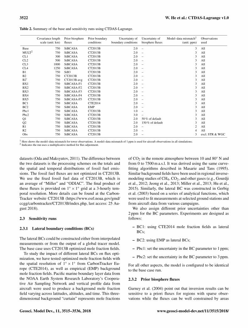
Table 2. Summary of the base and sensitivity runs using CTDAS-Lagrange.

Covariance length Prior biosphere Prior boundary Uncertainty of Uncertainty of Model–data mismatch1 Observationsscale (unit: km) fluxes conditions boundary conditions biosphere fluxes (unit: ppm) used

Base 750 SiBCASA CT2013B 2.0 – 3 AllMULT2 750 SiBCASA CT2013B 2.0 – 3 AllCL1 300 SiBCASA CT2013B 2.0 – 3 AllCL2 500 SiBCASA CT2013B 2.0 – 3 AllCL3 1000 SiBCASA CT2013B 2.0 – 3 AllCL4 1250 SiBCASA CT2013B 2.0 – 3 AllB1 750 SiB3 CT2013B 2.0 – 3 AllB2 750 CT2013B CT2013B 2.0 – 3 AllB2′ 750 CT2013B-avg CT2013B 2.0 – 3 AllBX1 750 SiBCASA-F1 CT2013B 2.0 – 3 AllBX2 750 SiBCASA-F2 CT2013B 2.0 – 3 AllBX3 750 SiBCASA-F3 CT2013B 2.0 – 3 AllBX4 750 SiBCASA-F4 CT2013B 2.0 – 3 AllBX5 750 SiBCASA-F5 CT2013B 2.0 – 3 AllBC1 750 SiBCASA CTE2014 2.0 – 3 AllBC2 750 SiBCASA EMP 2.0 – 3 AllPbc1 750 SiBCASA CT2013B 1.0 – 3 AllPbc2 750 SiBCASA CT2013B 3.0 – 3 AllQ1 750 SiBCASA CT2013B 2.0 50 % of default 3 AllQ2 750 SiBCASA CT2013B 2.0 150 % of default 3 AllR1 750 SiBCASA CT2013B 2.0 – 2 AllR2 750 SiBCASA CT2013B 2.0 – 4 AllObs 750 SiBCASA CT2013B 2.0 – 3 excl. STR & WGC

1 Here shows the model–data mismatch for tower observations. A model–data mismatch of 1 ppm is used for aircraft observations in all simulations;2 Indicates the run uses a multiplicative method for flux adjustment.

datasets (Oda and Maksyutov, 2011). The difference betweenthe two datasets is the processing schemes on the totals andthe spatial and temporal distributions of fossil fuel emis-sions. The fossil fuel fluxes are not optimized in CT2013B.We use the fixed fossil fuel data of CT2013B, which isan average of “Miller” and “ODIAC”. The final product ofthese fluxes is provided on 1◦× 1◦ grid at a 3-hourly tem-poral resolution. More details can be found at the Carbon-Tracker website CT2013B (https://www.esrl.noaa.gov/gmd/ccgg/carbontracker/CT2013B/index.php, last access: 25 Au-gust 2018).

2.3 Sensitivity runs

2.3.1 Lateral boundary conditions (BCs)

The lateral BCs could be constructed either from interpolatedmeasurements or from the output of a global tracer model.The base case uses CT2013B optimized mole fraction fields.

To study the impact of different lateral BCs on flux opti-mization, we have tested optimized mole fraction fields withthe spatial resolution of 1◦× 1◦ from CarbonTracker Eu-rope (CTE2014), as well as empirical (EMP) backgroundmole fraction fields. Pacific marine boundary layer data fromthe NOAA Earth System Research Laboratory’s Coopera-tive Air Sampling Network and vertical profile data fromaircraft were used to produce a background mole fractionfield varying across latitudes, altitudes, and time. This three-dimensional background “curtain” represents mole fractions

of CO2 in the remote atmosphere between 10 and 80◦ N andfrom 0 to 7500 m a.s.l. It was derived using the same curve-fitting algorithms described in Masarie and Tans (1995).Similar background fields have been used in regional inverse-modeling studies of CH4, CO2, and other gases (e.g., Gourdjiet al., 2012; Jeong et al., 2013; Miller et al., 2013; Hu et al.,2015). Similarly, the lateral BC was constructed in Gerbiget al. (2003) based on a series of analytical functions, whichwere used to fit measurements at selected ground stations andfrom aircraft data from various campaigns.

We also assign different prior uncertainties other than2 ppm for the BC parameters. Experiments are designed asfollows:

– BC1: using CTE2014 mole fraction fields as lateralBCs;

– BC2: using EMP as lateral BCs;

– Pbc1: set the uncertainty in the BC parameter to 1 ppm;

– Pbc2: set the uncertainty in the BC parameter to 3 ppm.

For all other aspects, the model is configured to be identicalto the base case run.

2.3.2 Prior biosphere fluxes

Gurney et al. (2004) point out that inversion results can besensitive to a priori fluxes for regions with sparse obser-vations while the fluxes can be well constrained by areas


https://www.esrl.noaa.gov/gmd/ccgg/carbontracker/CT2013B/index.php

https://www.esrl.noaa.gov/gmd/ccgg/carbontracker/CT2013B/index.php


with dense observations. To investigate the impact of dif-ferent a priori fluxes on the optimized fluxes, we have de-signed two sensitivity runs that incorporate two alternativebiosphere fluxes as a priori fluxes as follows:

– B1: SiB3 biosphere fluxes;

– B2: CT2013B optimized biosphere fluxes.

Except for the difference in the a priori biosphere fluxes,the two sensitivity runs share the same model setup as thebase case. SiB3 biosphere fluxes are the simulation resultsof the third version of the Simple Biosphere model (Bakeret al., 2008), with hourly fluxes and a spatial resolution of1◦× 1◦. CT2013B optimized biosphere fluxes are the out-puts of CT2013B that optimizes the global surface biospherefluxes, which uses higher-resolution transport over NorthAmerica than other regions. Although these fluxes are al-ready optimized against global and North American CO2observations, it is still interesting to optimize them in a dif-ferent assimilation system, especially when the system em-ploys a high spatial resolution and different transport model.In addition, CT2013B assimilates a different set of observa-tions compared to CTDAS-Lagrange. In principle, one ex-pects these fluxes to be most consistent with observations,and to lead to a very similar posterior mean flux as was pre-scribed through the prior.

For further analysis of the sensitivity of the CTDAS-Lagrange system to the annual mean and the seasonal mag-nitude of a priori fluxes, we have designed a series of runswith modified SiBCASA fluxes. We scaled the respirationof the SiBCASA fluxes while maintaining the gross primaryproduction (GPP) estimate to obtain a priori North Americanannual mean fluxes ranging from +0.43 to −2.06 PgC yr−1.The tests with prior fluxes+0.43,−0.06,−0.97,−1.44, and−2.06 PgC yr−1 are labeled with BX1, BX2, BX3, BX4, andBX5, respectively.

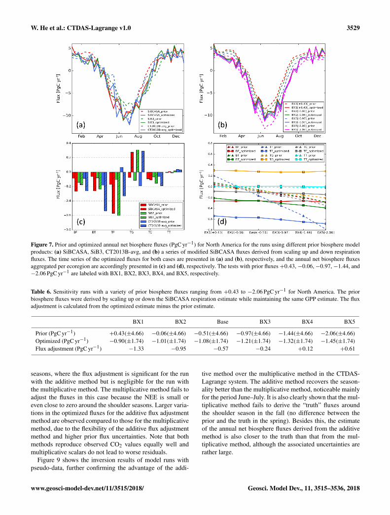
2.3.3 Additive or multiplicative flux adjustment

The multiplicative flux adjustment of NEE relates the uncer-tainties to the magnitude of the fluxes. As NEE is the dif-ference between two gross fluxes, gross primary productionand ecosystem respiration, 10-day mean NEE can be verysmall or even close to zero when GPP and respiration areclose to each other, e.g., in the so-called shoulder seasons(see Fig. 8), which limits the ability of using multiplicativeflux adjustment to scale the mean fluxes due to low uncer-tainties in the inversion system (note that the large diurnalcycle of the net flux will still be scaled though). Scaling bothGPP and respiration has been shown to circumvent this inderiving optimized mean fluxes (Tolk et al., 2011). Here, wehave instead implemented both multiplicative and additiveflux adjustment methods. For the multiplicative method, weset the biosphere scaling parameter variance as 80 %, follow-ing Peters et al. (2010); for the additive method, the vari-ance is prescribed as 1.6 µmol m−2 s−1 which represents the

typical flux uncertainty in the multiplicative method duringthe summer months. Because this value persists yearlong inthe additive run, the total annual uncertainty in this methodis higher though. Sensitivity tests for the covariance are de-scribed below. The additive method is used in the base caserun, and the multiplicative method was tested as a sensitivityrun.

For a better assessment of the adjusting ability of the twomethods, we further perform experimental inversions usingpseudo-data, i.e., Observing System Simulation Experiments(OSSEs). The primary aim of our OSSEs is to investigate theability of our system to retrieve surface fluxes given the ob-servational network. In particular, we test the implementationof the additive flux parameter vs. multiplicative flux parame-ter, and the ability to recover large biases in lateral BCs andprior fluxes. We run the CTDAS-Lagrange in a forward modewith the SiBCASA fluxes as prior to generate simulated molefractions, and then try to recover the “truth” in an inversionusing SiB3 fluxes as a priori.

2.3.4 Covariance length scales

The covariance length scale determines the rate at which thecorrelation between the fluxes of two grids within the sameecoregions decreases exponentially with increasing distance.The prescribed covariance effectively reduces the number ofunknowns to be solved for, and improves the ability of theinversion system to retrieve optimized fluxes when data arelimited (Rödenbeck et al., 2003; Gourdji et al., 2012). Thechoice of appropriate correlation length scale depends alsoon the observation density. For example, CarbonTracker Eu-rope, which includes more observations than those used inthis work, uses a correlation length scale of 300 km for NorthAmerica. In addition, Alden (2013) found 700 km to be thebest length scale to recover true fluxes over North Americawith a pseudo-data inversion experiment. To investigate theimpact of covariance length scales on optimized fluxes, weperformed sensitivity runs with a series of spatial correlationlengths: 300, 500, 750 km (base case), 1000, and 1250 km,labeled as CL1 to CL4, respectively.

2.3.5 Magnitude of covariance and model–datamismatch

Flux covariance determines the range in which prior bio-sphere fluxes can be adjusted. It should ideally reflect theuncertainty in prior biosphere fluxes, but information aboutprior flux errors is not readily available for the priors usedhere or for terrestrial ecosystem models more generally. Toevaluate the possible influence of prior covariances on theoptimized fluxes, we modified the additive uncertainty by±50 %. The model–data mismatch (MDM) is a parameterthat describes the capability of our modeling system to matchthe observations, and is used to de-weight observations thatare not well represented by the model simulations, e.g., in



Figure 3. Simulated CO2 (prior in red and optimized in green) and observed CO2 (black) for the Park Falls, Wisconsin, tower site (labeledLEF) for the year 2010. The blue squares (11 out of 409 samples) are rejected samples because the difference between simulated and observedCO2 is larger than 3 times the assigned model–data mismatch of 3 ppm for tower sites. The distribution of both prior and posterior residualsis presented on the right side. After optimization we observe a strong reduction of the CO2 mean bias and 1σ standard deviation from+0.85± 3.73 to +0.09± 1.55 ppm. Note that the prior residual distribution is calculated without the rejected observations, which explainsthe slightly different statistics in comparison to the data presented in Table 1.

the case of local influence. The observations are even ex-cluded when the differences between observed and simulatedCO2 are larger than 3 times the MDM. We set the MDM to3.0 ppm for tower sites and 1.0 ppm for aircraft sites. Thesensitivity tests that incorporate the covariance and MDM aredescribed below:

– Q1: decrease the magnitude of additive uncertainty by50 %, which means the covariance is 25 % of the de-fault;

– Q2: increase the magnitude of additive uncertainty by50 %, which means the covariance is 225 % of the de-fault;

– R1: set the MDM to 2 ppm for tower sites;

– R2: set the MDM to 4 ppm for tower sites.

The rest of the model setup is the same as the base case run.

2.3.6 Observational data choice

As a sensitivity test, we exclude observations at two towersites (STR and WGC), which are characterized with largerprior and posterior residuals (simulated minus observed, bothmean and standard deviation) than other sites. We have de-fined one sensitivity run as follows:

Obs: excluding STR and WGC, and the rest of the modelsetup is the same as the base case run.

3 Results

This section covers the following topics: CO2 mole fractionsimulations and seasonal cycles of biosphere fluxes from the

base case run, lateral BCs choice and optimization, sensi-tivity to a priori fluxes, additive or multiplicative adjustingparameters, covariance length scales, transport uncertainties,and a summary of ensemble estimates.

3.1 Observed and simulated CO2 mole fractions

As an example, a time series of simulated and observed CO2mole fractions at the LEF tower site for the year 2010 isshown in Fig. 3. As should be expected from the assimila-tion, the optimized CO2 records closely follow the CO2 ob-servations over time, and the optimized residuals (green) aresmaller than those from the model forecast (red). The dis-tribution of both prior and posterior residuals shown on theright side of Fig. 3 indicates improvement from the prior+0.85±3.73 ppm to the posterior 0.09±1.55 ppm. The largervariability in both observed and simulated CO2 between Mayand November (compared to the rest of the year) are likelycaused by larger variability in the biosphere fluxes duringthe growing season, as well as larger variation in atmosphericmixing conditions. A few simulated values (blue) are rejectedin the assimilation procedure because the difference betweensimulations with prior biosphere fluxes and observations islarger than 3 times the assigned model–data mismatch of3 ppm for tower sites. For the LEF tower site, 11 out of thetotal 409, or 2.9 % are rejected, which is slightly larger thanthe expected rejection rate (based on a 3σ cut-off for a Gaus-sian probability density function of the errors) of 2 % (Peterset al., 2010). It is shown in Table 1 that the rejection rates formost tower sites are around 2–3 %, except for WBI (7.6 %)and WGC (18.0 %).



3.2 Seasonal cycles of net ecosystem exchange (NEE) ofCO2

Figure 4 shows the seasonal cycle (10-day averages) of NEEof CO2 for the year 2010 for four major Olson aggregatedland-cover types of North America (Boreal Forests/Wooded,Boreal Tundra/Taiga, Temperate Forests/Wooded, and Tem-perate Crops/Agriculture). The amplitude of the seasonal cy-cle of temperate forests/wooded is the largest among the fourland-cover types, with both large summertime vegetative up-take and large wintertime respiratory emissions. Since thesame ecoregions may correspond to multiple regions and cli-mates, we have separated the southern and northern regionsfor crops and forests (divided by 40◦ N). The seasonal cyclesare mainly caused by those in the northern regions, especiallyfor crops. The uncertainties in the posterior fluxes have beenreduced for all four land-cover types and for almost all sea-sons of the year, especially for temperate forests/wooded andtemperate crops/agriculture.

The seasonal cycle of the posterior fluxes shows a simi-lar magnitude as the prior. In addition, the optimized fluxesgenerally show more fluctuations than prior fluxes over theyear, which could be explained by effective constraints fromatmospheric observations and possibly in some cases as ar-tifacts that are caused by the sparseness of the observations.It should be noted that it does not mean that the actual er-rors in these fluxes are really reduced, as this can only be as-sessed using independent observations of these fluxes. Withmonthly averaging, the fluctuations in the derived posteriorfluxes could be significantly reduced (see Fig. 4). Interest-ingly, the temperate crops/agriculture show double troughs inthe uptake in May and July–August or a sudden drop in theuptake in June, which could be attributed to early-summercrops/agriculture harvests, temperature anomaly, or drought.

The mean prior and optimized fluxes for the summermonths June–August are given in Fig. 5. The optimizedfluxes show a similar spatial pattern as the prior fluxes,but display more spatial details. The optimized results placemore carbon uptake in the agricultural US Midwest and theforests/wooded in the northeast of the US, as well as in theboreal forests/wooded and tundra/taiga of Canada; In con-trast, less carbon uptake (or carbon emissions) is placed inthe western US, especially in south Utah, north Arizona, andLouisiana.

3.3 Boundary condition choice and optimization

A comparison of the mole fraction contribution from threelateral BCs for the eight tower sites is summarized in Ta-ble 3. The annual means of the CTE2014 are consistently∼ 0.30 ppm higher than those of the CT2013B for all sites;however, the summertime means of the CTE2014 and theCT2013B are nearly equal except for the two sites AMTand STR. In contrast, the annual means of the EMP and theCT2013B are nearly equal for all sites; however, the summer-

time drawdowns of the EMP are significantly higher (−1.70to−0.28 ppm) than those of the CT2013B for all sites exceptSTR (0.66 ppm). This suggests that the two model-derivedBCs provide higher summer background mole fractions thanthe EMP-based background, which corresponds to a knownhigh bias in summertime CO2 across North America in bothversions of CarbonTracker used to construct the BCs.

The optimized annual mean fluxes and the adjustment ofthe BC parameters for the model runs with different prior lat-eral BCs are shown in Table 4. When both biosphere fluxesand BC parameters are optimized, i.e., “Flux+BC” optimiza-tion, the optimized annual mean fluxes using three differ-ent prior lateral BCs range from −1.26 to −1.08 PgC yr−1,with an average of −1.14± 0.10 PgC yr−1, which have asmaller variation compared to those from the model runswhen only biosphere fluxes are optimized, i.e., “Flux only”optimization, that ranges from −1.49 to −1.09 PgC yr−1 or−1.22± 0.23 PgC yr−1 (discussed in more detail in the fol-lowing section). The results show that the additional BC opti-mization is desired when model-based BCs are used, and thatthis reduces the annual mean optimized biosphere fluxes byup to 0.23 PgC yr−1, or 15.4 % of the “Flux only” optimizedfluxes. The largest adjustment in the optimized annual meanbiosphere uptake takes place in the run with the CTE2014as lateral BCs, which corresponds to the consistently higherannual means of the BC contributions of the CTE2014 thanthose of the CT2013B. The contribution of the adjustmentof BC parameters to simulated CO2 ranges from −0.18 to0.16 ppm over all seasons of the year 2010, which stressesthat this is a subtle, but systematic, signal to account for in aregional inversion.

The residuals of the model runs with and without BC op-timization (not shown), in almost all cases, are significantlyreduced after optimization. The reduction in the residuals af-ter optimization for aircraft sites is primarily due to the ad-justment of the BC parameters. We notice that the residuals(means and standard deviations) of the model runs with opti-mized biosphere fluxes and BC parameters for the two sitesSTR and WGC are larger than those for other sites. Possi-ble reasons are that the two sites are still significantly influ-enced by regional fossil fuel signals after the data filteringpresented in Sect. 2.1.3, and are less sensitive to biospherefluxes (due to their proximity to the west coast of NorthAmerica there is less sensitivity to land flux than for othersites). We will investigate the impact of the two observationsites on optimized fluxes in the following section.

The time series of optimized North American averagedbiosphere fluxes from the model runs with different prior lat-eral BCs are shown in Fig. 6. The differences among the op-timized fluxes with additional BC optimization (Fig. 6b) be-come smaller than those from the “Flux only” runs (Fig. 6a).This can also be observed when averaged over major ecore-gions (Fig. 6c and d), especially for the boreal forests andtemperate forests. The differences in the optimized biospherefluxes caused by different prior lateral BCs are mostly small,



Figure 4. The seasonal cycle (10-day resolution) of the net CO2 biosphere flux (PgC yr−1) of four aggregated Olson ecoregions in NorthAmerica for the year 2010. The prior biosphere flux (SiBCASA) and its uncertainty are displayed in blue, and the optimized biosphere fluxand uncertainty in black. “Optimized_sm” stands for the smoothed optimized fluxes (shown in red), which helps to remove the spuriousfluctuations. The Temperate Forests/Wooded and Crops/Agriculture are separated by 40◦ N into North and South, respectively.

Figure 5. Mean prior (a) and optimized (b) net biosphere fluxes, and the mean adjustment (optimized minus prior) (c) for summertime(June–July–August). Note that the color scale used in (c) is different from the one used in (a) and (b).

except that the deviation of the EMP optimized fluxes fromthe other two is slightly larger for the period July–September.

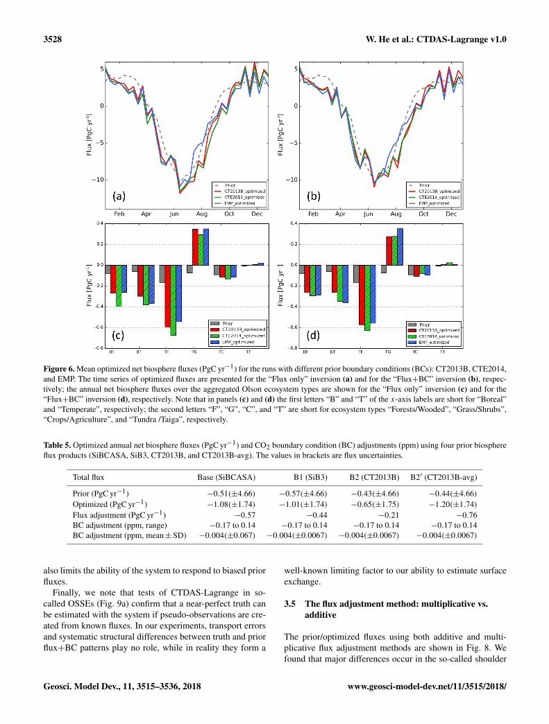
3.4 Sensitivity to prior biosphere fluxes

The optimized annual mean biosphere fluxes and associatedBC parameter adjustments from the runs with different priorbiosphere fluxes are shown in Table 5. The flux adjustmentsare in general large, resulting in significantly larger annualmean uptake over North America than the prior; however,the optimized annual mean fluxes from the runs using three

different prior biosphere products converge, except for therun using the original CT2013B optimized fluxes. A furthercheck indicates that the residuals of the run are reasonable,but more observations have been rejected compared with theother runs. The rejection takes place in the period from Juneto August, which is caused by large fluctuations of the a pri-ori fluxes. Note that the a priori CT2013B fluxes are opti-mized using weekly scaling factors in an assimilation win-dow of 5 weeks long and incur substantial variability (ornoise) that averages out over larger scales in CT2013B. But



Table 3. Contribution of lateral transport to simulated CO2 mole fractions at the tall tower network for three sets of lateral BCs. The meandifferences (in ppm) between CTE2014, EMP, and CT2013B BCs are calculated for 2010 and summer (JJA), respectively. The standarddeviation (1σ ) of the differences for each tower site is given in the parenthesis.

Site CTE2014 minus CT2013B EMP minus CT2013B

annual summer annual summer

AMT 0.39(±0.43) 0.49(±0.56) 0.04(±1.27) −1.19(±1.33)BAO 0.25(±0.34) −0.11(±0.35) −0.24(±1.26) −1.70(±1.54)LEF 0.36(±0.38) 0.00(±0.32) 0.05(±1.36) −1.07(±1.76)SCT 0.29(±0.37) 0.01(±0.40) −0.07(±1.19) −0.50(±1.16)STR 0.35(±0.52) 0.30(±0.19) −0.21(±1.58) 0.66(±0.78)WBI 0.39(±0.41) 0.16(±0.29) −0.03(±1.21) −0.28(±1.10)WGC 0.35(±0.39) −0.00(±0.34) −0.06(±1.30) −0.93(±1.80)WKT 0.31(±0.38) 0.16(±0.61) 0.14(±1.08) −0.66(±1.67)

Table 4. Comparison of the optimized annual net biosphere fluxes (PgC yr−1) and the adjustment of CO2 boundary conditions (BCs, ppm)using different prior lateral BC products (CT2013B, CTE2014, and EMP) and optimization techniques (“Flux only” or “Flux+BC”). Theannual net biosphere flux difference is calculated from the “Flux+BC” optimization minus “Flux only” optimization. The values in bracketsare flux uncertainties.

Total flux Base (CT2013B) BC1 (CTE2014) BC2 (EMP)

“Flux only” optimization (PgC yr−1) −1.10(±1.75) −1.49(±1.75) −1.09(±1.75)“Flux+BC” optimization (PgC yr−1) −1.08(±1.74) −1.26(±1.74) −1.09(±1.73)Flux difference (PgC yr−1) +0.02 +0.23 −0.00BC adjustment (ppm, range) −0.17 to 0.14 −0.18 to 0.16 −0.08 to 0.09BC adjustment (ppm, mean±SD) −0.004(±0.067) −0.004(±0.078) −0.001(±0.030)

the forward simulations of the CTDAS-Lagrange system aresensitive to the fluxes and their diurnal cycle is only in a 10-day window and therefore more sensitive to this variability(or noise). Therefore, we have made an additional sensitivitytest (B2′) with smoothed CT2013B fluxes (10-day averaged,identical 3-hourly fluxes across a day in every 10-day period)as a priori, which gives smaller optimized annual fluxes (seeTable 5). Because the prior CT2013B fluxes contain largefluctuations, we have averaged the fluxes within 10-day win-dows to a single constant value. We are fully aware that thisis not realistic, and this should be regarded as a sensitivitytest to understanding the difficulties of our CTDAS-Lagrangesystem to high-frequency fluctuations in the prior fluxes withlimited flexibility (prior flux uncertainty). We hereafter referto CT2013B-avg for further analysis.

Figure 7a shows the time series of the North American av-eraged biosphere fluxes of the model runs with different priorbiosphere fluxes. It is noticeable that the difference in the sea-sonal amplitude between the SiB3 prior biosphere fluxes andthe other two prior biosphere fluxes is diminished after opti-mization. Furthermore, the significant difference among thethree prior products for the period August–October is largelyreconciled by the inversion. Annual mean fluxes per ecore-gion (Fig. 7c) indicate that the largest adjustment in the fluxestakes place for temperate forests and temperate grass, withfluxes from temperate grass changed from uptake to emis-

sions. Note that the optimized fluxes per ecoregion do notalways agree on their magnitudes, which is likely caused byinsufficient constraints by observations, especially for the bo-real region.

To further investigate the sensitivity of the CTDAS-Lagrange system to the seasonal magnitude and the annualmean of a priori fluxes, we scale the respiration of the SiB-CASA fluxes to obtain a variety of a priori fluxes with theannual mean NEE ranging from +0.43 to −2.06 PgC yr−1.We find that the seasonal magnitudes of the optimized fluxesare nearly independent of those of the prior fluxes (Fig. 7b),and the range of the annual mean is significantly reduced to−0.9 to −1.45 PgC yr−1 (Table 6). Like the runs with theprior fluxes from SiBCASA, SiB3 and CT2013B-avg, theoptimized fluxes show variations at multiple times of theyear that are a direct result of the corresponding flux ad-justment within 10-day windows. The prior/optimized fluxesper ecoregion (Fig. 7d) show that the optimized fluxes areeither independent of (e.g., boreal forests/wooded, temper-ate grass/shrubs) or have a slight dependence on (e.g., bo-real tundra/taiga, temperate forests/wooded) the priors. Thisdemonstrates that the CTDAS-Lagrange system can resolvelarge biases in the priors, but the magnitude of adjustmentis also limited by the prescribed flux uncertainty, which isconfirmed by the tests with increased flux uncertainty (notshown). Besides this, the limited choice of data constraints



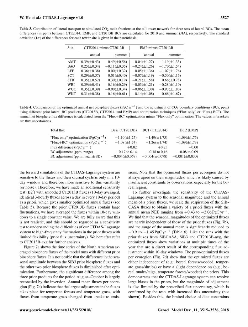
Figure 6. Mean optimized net biosphere fluxes (PgC yr−1) for the runs with different prior boundary conditions (BCs): CT2013B, CTE2014,and EMP. The time series of optimized fluxes are presented for the “Flux only” inversion (a) and for the “Flux+BC” inversion (b), respec-tively; the annual net biosphere fluxes over the aggregated Olson ecosystem types are shown for the “Flux only” inversion (c) and for the“Flux+BC” inversion (d), respectively. Note that in panels (c) and (d) the first letters “B” and “T” of the x-axis labels are short for “Boreal”and “Temperate”, respectively; the second letters “F”, “G”, “C”, and “T” are short for ecosystem types “Forests/Wooded”, “Grass/Shrubs”,“Crops/Agriculture”, and “Tundra /Taiga”, respectively.

Table 5. Optimized annual net biosphere fluxes (PgC yr−1) and CO2 boundary condition (BC) adjustments (ppm) using four prior biosphereflux products (SiBCASA, SiB3, CT2013B, and CT2013B-avg). The values in brackets are flux uncertainties.

Total flux Base (SiBCASA) B1 (SiB3) B2 (CT2013B) B2′ (CT2013B-avg)

Prior (PgC yr−1) −0.51(±4.66) −0.57(±4.66) −0.43(±4.66) −0.44(±4.66)Optimized (PgC yr−1) −1.08(±1.74) −1.01(±1.74) −0.65(±1.75) −1.20(±1.74)Flux adjustment (PgC yr−1) −0.57 −0.44 −0.21 −0.76BC adjustment (ppm, range) −0.17 to 0.14 −0.17 to 0.14 −0.17 to 0.14 −0.17 to 0.14BC adjustment (ppm, mean±SD) −0.004(±0.067) −0.004(±0.0067) −0.004(±0.0067) −0.004(±0.0067)

also limits the ability of the system to respond to biased priorfluxes.

Finally, we note that tests of CTDAS-Lagrange in so-called OSSEs (Fig. 9a) confirm that a near-perfect truth canbe estimated with the system if pseudo-observations are cre-ated from known fluxes. In our experiments, transport errorsand systematic structural differences between truth and priorflux+BC patterns play no role, while in reality they form a

well-known limiting factor to our ability to estimate surfaceexchange.

3.5 The flux adjustment method: multiplicative vs.additive

The prior/optimized fluxes using both additive and multi-plicative flux adjustment methods are shown in Fig. 8. Wefound that major differences occur in the so-called shoulder



Figure 7. Prior and optimized annual net biosphere fluxes (PgC yr−1) for North America for the runs using different prior biosphere modelproducts: (a) SiBCASA, SiB3, CT2013B-avg, and (b) a series of modified SiBCASA fluxes derived from scaling up and down respirationfluxes. The time series of the optimized fluxes for both cases are presented in (a) and (b), respectively, and the annual net biosphere fluxesaggregated per ecoregion are accordingly presented in (c) and (d), respectively. The tests with prior fluxes +0.43, −0.06, −0.97, −1.44, and−2.06 PgC yr−1 are labeled with BX1, BX2, BX3, BX4, and BX5, respectively.

Table 6. Sensitivity runs with a variety of prior biosphere fluxes ranging from +0.43 to −2.06 PgC yr−1 for North America. The priorbiosphere fluxes were derived by scaling up or down the SiBCASA respiration estimate while maintaining the same GPP estimate. The fluxadjustment is calculated from the optimized estimate minus the prior estimate.

BX1 BX2 Base BX3 BX4 BX5

Prior (PgC yr−1) +0.43(±4.66) −0.06(±4.66) −0.51(±4.66) −0.97(±4.66) −1.44(±4.66) −2.06(±4.66)Optimized (PgC yr−1) −0.90(±1.74) −1.01(±1.74) −1.08(±1.74) −1.21(±1.74) −1.32(±1.74) −1.45(±1.74)Flux adjustment (PgC yr−1) −1.33 −0.95 −0.57 −0.24 +0.12 +0.61

seasons, where the flux adjustment is significant for the runwith the additive method but is negligible for the run withthe multiplicative method. The multiplicative method fails toadjust the fluxes in this case because the NEE is small oreven close to zero around the shoulder seasons. Larger varia-tions in the optimized fluxes for the additive flux adjustmentmethod are observed compared to those for the multiplicativemethod, due to the flexibility of the additive flux adjustmentmethod and higher prior flux uncertainties. Note that bothmethods reproduce observed CO2 values equally well andmultiplicative scalars do not lead to worse residuals.

Figure 9 shows the inversion results of model runs withpseudo-data, further confirming the advantage of the addi-

tive method over the multiplicative method in the CTDAS-Lagrange system. The additive method recovers the season-ality better than the multiplicative method, noticeable mainlyfor the period June–July. It is also clearly shown that the mul-tiplicative method fails to derive the “truth” fluxes aroundthe shoulder season in the fall (no difference between theprior and the truth in the spring). Besides this, the estimateof the annual net biosphere fluxes derived from the additivemethod is also closer to the truth than that from the mul-tiplicative method, although the associated uncertainties arerather large.



Figure 8. Comparison between two flux optimization methods: the additive method (a) gives significant different optimized fluxes, high-lighted by the red dashed ellipses, in contrast to the multiplicative method (b), and (c) is similar to (b) but with 2 times the flux uncertainty,i.e., setting the biosphere scaling parameter variance to 160 %. The additive method seems more flexible to adjust fluxes in case net carbonexchange is small or even close to zero around the shoulder seasons (spring/fall).

Figure 9. Comparison of the performance of inversions with pseudo-data using the two flux optimization methods: (a) the additive methodand (b) the multiplicative method, (c) is similar to (b) but with 2 times the flux uncertainty, i.e., setting the biosphere scaling parametervariance to 160 %. The “truth” fluxes are generated in a forward simulation using biosphere fluxes from SiBCASA. The same SiB3 fluxesare used as a priori for all runs. The annual net biosphere fluxes of the truth, prior, and optimized are given in the legend, with the unit ofPgC yr−1.

Figure 10. Sensitivity of the optimized annual net biosphere fluxes(PgC yr−1) as a function of the chosen covariance length scale (km).The optimized fluxes tend to converge to −1.1 PgC yr−1 when thelength scale is larger than 750 km.

3.6 Sensitivity to the covariance length scale

The sensitivity of the CTDAS-Lagrange to the covariancelength scale is shown in Fig. 10. The optimized fluxes tendto reach a robust value when the covariance length scale islarger than 750–1000 km, and we note that the difference be-

tween 750 and 1000 km is relatively small. We have testedwhether including aircraft sites can reduce this length scaledependence below 1000 km, and find it can slightly allevi-ate the dependence but does not fully resolve that. The opti-mized fluxes for the temperate North America are relativelyinsensitive to the covariance length scale, as this region isrelatively well sampled by the dataset. We have only usedsome of the available observations, and different results maybe found when additional data are included, e.g., from Envi-ronment Canada tower sites.

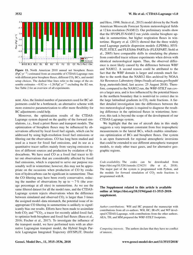
3.7 Ensemble estimates

From the above-described sensitivity runs, we derive an en-semble of estimates of optimized North American annual netbiosphere fluxes in 2010 (see Fig. 11). The optimized bio-sphere fluxes of all the runs are larger (i.e., more uptake) thantheir corresponding prior fluxes. Compared to other factors,the prior biosphere fluxes have the largest impact on the opti-mization result. The selection of model–data mismatch with3 ppm is reasonable, judging from the observed small dif-ferences between the model runs BASE and R2 (4 ppm). We



notice the R1 (2 ppm) run makes a significant difference, as itrejects much more observations than the other two cases, es-pecially during summertime when usually larger mismatchesbetween observations and simulations occurred (not shown).

Comparing BASE, Q1 (decrease the magnitude of addi-tive uncertainty by 50 %), and Q2 (increase the magnitude ofadditive uncertainty by 50 %), we find the prior uncertaintymagnitude ascribed to biosphere fluxes impacts the resultonly a little, with small reductions in the optimized flux whenthe uncertainty gets larger. In addition, we find that our sys-tem is sensitive to the uncertainty in the BC parameter Pbc1(1 ppm uncertainty) and Pbc2 (3 ppm uncertainty), which re-sults in the difference of flux estimates by slightly more than0.1 PgC yr−1. The choice of 2 ppm is according to the un-certainties we assessed from the statistics between these dif-ferent prior BCs we used. When the two tower sites STRand WGC that are located close to the west coast of NorthAmerica are excluded, we find smaller biosphere fluxes (thedifference is approximately 0.15 PgC yr−1), which indicatesthat attention should be paid to the choice of the observations.

Excluding results from B2 that we consider unrealistic dueto the high data rejection rate (replaced by the B2′ run), weestimate North American carbon fluxes for the year 2010 tobe between −0.92 and −1.26 PgC yr−1.

4 Conclusions and discussion

We have implemented a regional carbon assimilation sys-tem based on the CarbonTracker Data Assimilation Shellframework and a high-resolution Lagrangian transport modelWRF-STILT. The new system, named CTDAS-Lagrange,optimizes both biosphere fluxes and four boundary condi-tion (BC) parameters and is computationally efficient (1 yearof optimization can be performed serially within 14 h witheight threads on a 12-core Intel Xeon processor E5 v2 familycomputer with a processor base frequency of 2.7 GHz, oncefootprints are calculated and stored offline). Furthermore, wehave demonstrated that the additive flux adjustment methodis more flexible in optimizing NEE than the multiplicativeflux adjustment method, especially in the shoulder seasonsof the year.

The sensitivity test results with three different lateral BCs(CT2013B, CTE2014, and an empirical curtain) indicate thatCTDAS-Lagrange has the ability to largely correct for thepotential biases in the lateral BCs, with the BC optimizationabsorbing up to 0.23 PgC yr−1 of flux adjustment that wouldotherwise have been made to the optimized annual net bio-sphere fluxes. This makes the CTDAS-Lagrange system lessdependent on the choice of lateral BCs than a system withoutBC optimization or offline correction. The sensitivity testswith two alternative biosphere fluxes (SiB3 and CT2013B-avg) and a series of modified SiBCASA fluxes with a largerange of NEE show that the seasonal magnitude of the op-timized fluxes is almost independent of the prior fluxes, and

the optimized annual net biosphere fluxes converge for SiB3and CT2013B-avg and are much less dependent on the rangeof the priors for the series of modified SiBCASA fluxes. Thisdemonstrates that the CTDAS-Lagrange system is capableof resolving large biases in the prior biosphere fluxes. Onthe other hand, the optimized annual net biosphere fluxeswith different prior fluxes are less convergent at the ecore-gion level, presumably due to the limited choice of obser-vational constraints. This could also be improved by betterprescribing the uncertainties in biosphere fluxes for the ad-ditive adjustment method, as the assumption of spatially andtemporally uniform flux uncertainties may not be reasonable.

We derive an ensemble of estimates of the optimizedannual net biosphere carbon fluxes based on a series ofsensitivity tests, which places the North American Carbonsink for the year 2010 at −0.92 to −1.26 PgC yr−1, com-parable to the TM5-based estimates of CarbonTracker (ver-sion CT2016, −0.91± 1.10 PgC yr−1, data obtained fromhttps://www.esrl.noaa.gov/gmd/ccgg/carbontracker/, last ac-cess: 25 August 2018) and CarbonTracker Europe (versionCTE2016, −0.91± 0.31 PgC yr−1; van der Laan-Luijkx etal., 2017). Note that much less observations have been usedin CTDAS-Lagrange than those assimilated in CT2016 andCTE2016. This work is to be followed up by a multi-yearinversion using more available observations in recent years,and by assimilating an additional tracer, carbonyl sulfide, tosimultaneously constrain both GPP and NEE.

In addition, the estimate of net CO2 uptake for theyear 2010 is reasonable compared to an ensemble of atmo-spheric inversions from several studies that place the NorthAmerican NEE for 2000–2006 at −0.931± 0.670 PgC yr−1

(Hayes et al., 2012), and a more recent study suggestingthe North American net CO2 biosphere fluxes during 2000–2009 to be −0.890± 0.400 PgC yr−1 from the RECCAP-selected TransCom3 inversions (King et al., 2015). Threeatmospheric inversion studies placed North American NEEfor the year 2004, which had been recognized as a climate-favorable year for uptake, from −0.953±0.106 to−1.230±1.120 PgC yr−1 (CT2011, Peters et al., 2007; Butler et al.,2010; Gourdji et al., 2012). However, we also note that al-though we have a comparable estimate to the two versionsof CarbonTracker at the continental scale, our estimates atecoregion scales are different. Typically the boreal region isnot well constrained in our study with eight tower sites lo-cated in the US, while no data from the extensive network ofEnvironment Canada was used. To solve finer-scale fluxes,the use of data from a denser observational network is de-sirable and could likely further reduce the chosen covariancelength scale shown in Fig. 10.

Although we have accounted for the impact of possible bi-ases in the prior lateral BCs on optimized fluxes, we find thatthere remains room to further reduce the biases at surfacesites (shown in Table 1 as posterior residuals). This couldbe partially because aircraft observations are sparse, and aretemporally insufficient for sampling the inflows of the conti-


https://www.esrl.noaa.gov/gmd/ccgg/carbontracker/


Figure 11. North American 2010 annual net biosphere fluxes(PgC yr−1) estimated from an ensemble of CTDAS-Lagrange runswith different prior biosphere fluxes, different CO2 BCs, and modelsetup choices. The dashed blue lines refer to the range of the en-semble estimates −0.92 to −1.26 PgC yr−1 excluding the B2 run.See Table 2 for an overview of all experiments.

nent. Also, the limited number of parameters used for BC ad-justments could be a bottleneck; an alternative scheme withmore extensive parameterization to offer more flexibility forBC adjustments could help.

Moreover, the optimization results of the CTDAS-Lagrange system depend on the quality of the forward sim-ulations, i.e., fixed a priori fluxes and transport models. Theoptimization of biosphere fluxes may be influenced by ob-servations affected by local fossil fuel signals, which can beaddressed by using high-resolution fossil fuel emissions orfiltering out the observations. CO has long been studied andused as a tracer for fossil fuel emissions, and its use as aquantitative tracer suffers mainly from varying emission ra-tios of different sources and production by oxidation of hy-drocarbons. We have used CO as a fossil fuel tracer to fil-ter out observations that are considerably affected by fossilfuel emissions, which is expected to serve our purpose rea-sonably well in wintertime; however, this may not be appro-priate on the occasions when production of CO by oxida-tion of hydrocarbons can be significant in summertime. Thusthe CO filtering may have been overly conservative, reduc-ing the number of observations by up to ∼ 7 % (the aver-age percentage at all sites) in summertime. As we use thesame filtered dataset for all the model runs, and the CTDAS-Lagrange system rejects observations when the differencebetween simulated and observed CO2 is larger than 3 timesthe assigned model–data mismatch, the potential issue of in-appropriate CO filtering in summertime is unlikely to signif-icantly bias our results. Efforts have been made to assimilateboth CO2 and 14CO2, a tracer for recently added fossil fuel,to optimize both biosphere and fossil fuel fluxes (Basu et al.,2016; Fischer et al., 2017). To investigate the influence ofthe transport model, we have performed tests with an alter-native Lagrangian transport model, the Hybrid Single Par-ticle Lagrangian Integrated Trajectory (HYSPLIT; Draxler

and Hess, 1998; Stein et al., 2015) model driven by the NorthAmerican Mesoscale Forecast System meteorological fieldsat 12 km resolution (NAM12). Our preliminary results showthat the HYSPLIT-NAM12 run yields similar biosphere up-take in summertime, but higher respiration fluxes in win-tertime. Hegarty et al. (2013) showed that the three widelyused Lagrange particle dispersion models (LPDMs), HYS-PLIT, STILT, and FLEXible PARTicle (FLEXPART; Stohl etal., 2005) have comparable skills in simulating the plumesfrom controlled tracer release experiments when driven withidentical meteorological inputs. Thus, the observed differ-ence is most likely caused by the difference between WRFand NAM12. A second reason could be attributed to thefact that the WRF domain is larger and extends much fur-ther to the north than the NAM12 files archived by NOAAAir Resources Laboratory (https://ready.arl.noaa.gov/hypub/hysp_meteoinfo.html, last access: 25 August 2018). There-fore, compared to the NAM12 run, the WRF-STILT run cov-ers a larger area, and is less influenced by the potential biasesin the northern boundary that is nontrivial to correct due tothe large latitudinal gradients in CO2 mole fractions. A fur-ther detailed investigation into the differences between thetwo meteorological inputs is required to diagnose the result-ing difference in the optimized fluxes in wintertime; how-ever, this task is beyond the scope of the development of ourCTDAS-Lagrange system.

We highlight that the use of aircraft data in this studysuggests a very important constraint from free troposphericmeasurements to the lateral BCs, which enables simultane-ous optimization of BCs and biosphere fluxes. Our systemis an open framework for regional atmospheric inversionsthat could be extended to use different atmospheric transportmodels, to study other trace gases, and for alternative geo-graphic regions.

Code availability. The codes can be downloaded fromhttps://doi.org/10.5281/zenodo.1234231 (He et al., 2018).The major part of the system is programmed with Python, andthe module for forward simulation of CO2 mole fractions isprogrammed with R.

The Supplement related to this article is availableonline at https://doi.org/10.5194/gmd-11-3515-2018-supplement.

Author contributions. WH and HC prepared the manuscript withcontributions from all co-authors. WH, HC, IRvdV, and WP devel-oped CTDAS-Lagrange, with contributions from the other authors.AEA, TH, and MM prepared the WRF-STILT footprints.

Competing interests. The authors declare that they have no conflictof interest.


https://ready.arl.noaa.gov/hypub/ hysp_meteoinfo.html

https://ready.arl.noaa.gov/hypub/ hysp_meteoinfo.html

https://doi.org/10.5281/zenodo.1234231

https://doi.org/10.5194/gmd-11-3515-2018-supplement

https://doi.org/10.5194/gmd-11-3515-2018-supplement


Acknowledgements. This research is funded by the NOAA ClimateProgram Office’s AC4 program (award number NA13OAR4310082and additional support for production of the NOAA CarbonTrackerLagrange footprint library), and by the National Key R&DProgram of China (2016YFA0600202). Wouter Peters was par-tially funded from European Research Council grant 649087(ASICA). Ingrid T. van der Laan-Luijkx is funded by a NWO Venigrant (016.Veni.171.095). Data collection at Walnut Grove andSutro towers was partially supported by the California Energy Com-missions’s Natural Gas Research Program and the California AirResources Board at Lawrence Berkeley National Laboratory underUS Department of Energy contract no. DE-AC02-05CH11231. Weare grateful to Ian Baker for providing the SiB3 fluxes, to AndyJacobson for his useful comments on the manuscript, and for theIT support at the Centre for Isotope Research of the University ofGroningen.

Edited by: Philippe PeylinReviewed by: two anonymous referees

References

Alden, C. B.: Terrestrial carbon cycle responses to drought and cli-mate stress: new insights using atmospheric observations of CO2and δ13C, Dissertations & Theses, Gradworks, 167–196, 2013.

Alden, C. B., Miller, J. B., Gatti, L. V., Gloor, M. M., Guan, K.,Michalak, A. M., van der Laan-Luijkx, I. T., Touma, D., An-drews, A., Basso, L. S., Correia, C. S. C., Domingues, L. G.,Joiner, J., Krol, M. C., Lyapustin, A. I., Peters, W., Shiga, Y.P., Thoning, K., van der Velde, I. R., van Leeuwen, T. T., Ya-dav, V., and Diffenbaugh, N. S.: Regional atmospheric CO2 in-version reveals seasonal and geographic differences in Ama-zon net biome exchange, Glob. Change Biol., 22, 3427–3443,https://doi.org/10.1111/gcb.13305, 2016.

Andersson, E., Kahnert, M., and Devasthale, A.: Methodology forevaluating lateral boundary conditions in the regional chemicaltransport model MATCH (v5.5.0) using combined satellite andground-based observations, Geosci. Model Dev., 8, 3747–3763,https://doi.org/10.5194/gmd-8-3747-2015, 2015.

Andrews, A. E., Kofler, J. D., Trudeau, M. E., Williams, J. C., Neff,D. H., Masarie, K. A., Chao, D. Y., Kitzis, D. R., Novelli, P. C.,Zhao, C. L., Dlugokencky, E. J., Lang, P. M., Crotwell, M. J.,Fischer, M. L., Parker, M. J., Lee, J. T., Baumann, D. D., Desai,A. R., Stanier, C. O., De Wekker, S. F. J., Wolfe, D. E., Munger,J. W., and Tans, P. P.: CO2, CO, and CH4 measurements from talltowers in the NOAA Earth System Research Laboratory’s GlobalGreenhouse Gas Reference Network: instrumentation, uncer-tainty analysis, and recommendations for future high-accuracygreenhouse gas monitoring efforts, Atmos. Meas. Tech., 7, 647–687, https://doi.org/10.5194/amt-7-647-2014, 2014.

Baker, I. T., Prihodko, L., Denning, A. S., Goulden, M., Miller, S.,and da Rocha, H. R.: Seasonal drought stress in the Amazon:Reconciling models and observations, J. Geophys. Res.-Biogeo.,113, G00b01, https://doi.org/10.1029/2007jg000644, 2008.

Basu, S., Miller, J. B., and Lehman, S.: Separation of biosphericand fossil fuel fluxes of CO2 by atmospheric inversion of CO2and 14CO2 measurements: Observation System Simulations, At-

mos. Chem. Phys., 16, 5665–5683, https://doi.org/10.5194/acp-16-5665-2016, 2016.

Bergamaschi, P., Krol, M., Meirink, J. F., Dentener, F., Segers, A.,van Aardenne, J., Monni, S., Vermeulen, A. T., Schmidt, M.,Ramonet, M., Yver, C., Meinhardt, F., Nisbet, E. G., Fisher, R.E., O’Doherty, S., and Dlugokencky, E. J.: Inverse modeling ofEuropean CH4 emissions 2001–2006, J. Geophys. Res.-Atmos.,115, D22309, https://doi.org/10.1029/2010JD014180, 2010.

Brioude, J., Angevine, W. M., Ahmadov, R., Kim, S.-W., Evan, S.,McKeen, S. A., Hsie, E.-Y., Frost, G. J., Neuman, J. A., Pol-lack, I. B., Peischl, J., Ryerson, T. B., Holloway, J., Brown,S. S., Nowak, J. B., Roberts, J. M., Wofsy, S. C., Santoni, G.W., Oda, T., and Trainer, M.: Top-down estimate of surface fluxin the Los Angeles Basin using a mesoscale inverse modelingtechnique: assessing anthropogenic emissions of CO, NOx andCO2 and their impacts, Atmos. Chem. Phys., 13, 3661–3677,https://doi.org/10.5194/acp-13-3661-2013, 2013.

Broquet, G., Chevallier, F., Bréon, F.-M., Kadygrov, N., Alemanno,M., Apadula, F., Hammer, S., Haszpra, L., Meinhardt, F., Morguí,J. A., Necki, J., Piacentino, S., Ramonet, M., Schmidt, M.,Thompson, R. L., Vermeulen, A. T., Yver, C., and Ciais, P.:Regional inversion of CO2 ecosystem fluxes from atmosphericmeasurements: reliability of the uncertainty estimates, Atmos.Chem. Phys., 13, 9039–9056, https://doi.org/10.5194/acp-13-9039-2013, 2013.

Butler, M. P., Davis, K. J., Denning, A. S., and Kawa, S. R.: Us-ing continental observations in global atmospheric inversionsof CO2: North American carbon sources and sinks, Tellus B,62, 550–572, https://doi.org/10.1111/j.1600-0889.2010.00501.x,2010.

Chevallier, F., Ciais, P., Conway, T. J., Aalto, T., Anderson, B. E.,Bousquet, P., Brunke, E. G., Ciattaglia, L., Esaki, Y., Froehlich,M., Gomez, A., Gomez-Pelaez, A. J., Haszpra, L., Krummel, P.B., Langenfelds, R. L., Leuenberger, M., Machida, T., Maignan,F., Matsueda, H., Morgui, J. A., Mukai, H., Nakazawa, T., Peylin,P., Ramonet, M., Rivier, L., Sawa, Y., Schmidt, M., Steele, L. P.,Vay, S. A., Vermeulen, A. T., Wofsy, S., and Worthy, D.: CO2 sur-face fluxes at grid point scale estimated from a global 21 year re-analysis of atmospheric measurements, J. Geophys. Res.-Atmos.,115, D21307, https://doi.org/10.1029/2010JD013887, 2010.

Conway, T. J., Tans, P. P., Waterman, L. S., and Thoning, K.W.: Evidence for Interannual Variability of the Carbon-Cyclefrom the National-Oceanic-and-Atmospheric-AdministrationClimate-Monitoring-and-Diagnostics-Laboratory Global-Air-Sampling-Network, J. Geophys. Res.-Atmos., 99, 22831–22855,1994.

Corazza, M., Bergamaschi, P., Vermeulen, A. T., Aalto, T.,Haszpra, L., Meinhardt, F., O’Doherty, S., Thompson, R.,Moncrieff, J., Popa, E., Steinbacher, M., Jordan, A., Dlugo-kencky, E., Brühl, C., Krol, M., and Dentener, F.: Inverse mod-elling of European N2O emissions: assimilating observationsfrom different networks, Atmos. Chem. Phys., 11, 2381–2398,https://doi.org/10.5194/acp-11-2381-2011, 2011.

Draxler, R. R. and Hess, G. D.: An overview of the HYSPLIT_4modelling system for trajectories, dispersion and deposition,Aust. Meteorol. Mag., 47, 295–308, 1998.

Fischer, M. L., Parazoo, N., Brophy, K., Cui, X., Jeong, S., Liu,J., Keeling, R., Taylor, T. E., Gurney, K., Oda, T., and Graven,H.: Simulating estimation of California fossil fuel and biosphere


https://doi.org/10.1111/gcb.13305

https://doi.org/10.5194/gmd-8-3747-2015

https://doi.org/10.5194/amt-7-647-2014

https://doi.org/10.1029/2007jg000644

https://doi.org/10.5194/acp-16-5665-2016

https://doi.org/10.5194/acp-16-5665-2016

https://doi.org/10.1029/2010JD014180

https://doi.org/10.5194/acp-13-3661-2013

https://doi.org/10.5194/acp-13-9039-2013

https://doi.org/10.5194/acp-13-9039-2013

https://doi.org/10.1111/j.1600-0889.2010.00501.x

https://doi.org/10.1029/2010JD013887

https://doi.org/10.5194/acp-11-2381-2011


carbon dioxide exchanges combining in situ tower and satellitecolumn observations, J. Geophys. Res.-Atmos., 122, 3653–3671,https://doi.org/10.1002/2016JD025617, 2017.

Gerbig, C., Lin, J. C., Wofsy, S. C., Daube, B. C., Andrews, A.E., Stephens, B. B., Bakwin, P. S., and Grainger, C. A.: Towardconstraining regional-scale fluxes of CO2 with atmospheric ob-servations over a continent: 2. Analysis of COBRA data usinga receptor-oriented framework, J. Geophys. Res.-Atmos., 108,4757, https://doi.org/10.1029/2003jd003770, 2003.

Giglio, L., van der Werf, G. R., Randerson, J. T., Collatz, G.J., and Kasibhatla, P.: Global estimation of burned area usingMODIS active fire observations, Atmos. Chem. Phys., 6, 957–974, https://doi.org/10.5194/acp-6-957-2006, 2006.

Göckede, M., Turner, D. P., Michalak, A. M., Vickers, D., and Law,B. E.: Sensitivity of a subregional scale atmospheric inverse CO2modeling framework to boundary conditions, J. Geophys. Res.-Atmos., 115, D24112, https://doi.org/10.1029/2010JD014443,2010.

Gourdji, S. M., Mueller, K. L., Yadav, V., Huntzinger, D.N., Andrews, A. E., Trudeau, M., Petron, G., Nehrkorn, T.,Eluszkiewicz, J., Henderson, J., Wen, D., Lin, J., Fischer, M.,Sweeney, C., and Michalak, A. M.: North American CO2 ex-change: inter-comparison of modeled estimates with results froma fine-scale atmospheric inversion, Biogeosciences, 9, 457–475,https://doi.org/10.5194/bg-9-457-2012, 2012.

Gurney, K. R., Law, R. M., Denning, A. S., Rayner, P. J., Pak, B.C., Baker, D., Bousquet, P., Bruhwiler, L., Chen, Y. H., Ciais,P., Fung, I. Y., Heimann, M., John, J., Maki, T., Maksyutov, S.,Peylin, P., Prather, M., and Taguchi, S.: Transcom 3 inversion in-tercomparison: Model mean results for the estimation of seasonalcarbon sources and sinks, Global Biogeochem. Cy., 18, GB1010,https://doi.org/10.1029/2003GB002111, 2004.

Hayes, D. J., Turner, D. P., Stinson, G., McGuire, A. D., Wei,Y., West, T. O., Heath, L. S., Dejong, B., McConkey, B. G.,Birdsey, R. A., Kurz, W. A., Jacobson, A. R., Huntzinger,D. N., Pan, Y., Mac Post, W., and Cook, R. B.: Reconcil-ing estimates of the contemporary North American carbon bal-ance among terrestrial biosphere models, atmospheric inversions,and a new approach for estimating net ecosystem exchangefrom inventory-based data, Glob. Change Biol., 18, 1282–1299,https://doi.org/10.1111/j.1365-2486.2011.02627.x, 2012.

He, W., van der Velde, I. R., Andrews, A. E., Sweeney,C., Miller, J., Tans,P., and Chen, H.: njuhewei/CTDAS-Lagrange: CTDAS-Lagrange (Version v1.0.0). Ctdas-lagrange V1.0: A High-resolution Data Assimilation Sys-tem for Regional Carbon Dioxide Observations, Zenodo,https://doi.org/10.5281/zenodo.1234231, 2018.

Hegarty, J., Draxler, R. R., Stein, A. F., Brioude, J., Mountain,M., Eluszkiewicz, J., Nehrkorn, T., Ngan, F., and Andrews, A.:Evaluation of Lagrangian Particle Dispersion Models with Mea-surements from Controlled Tracer Releases, J. Appl. Meteo-rol. Clim., 52, 2623–2637, https://doi.org/10.1175/JAMC-D-13-0125.1, 2013.

Houghton, J. T., Ding, Y., Griggs, D. J., Norguer, M., van der Lin-den, P. J., Dai, X., Maskell, K., and Johnson, C. A.: Climatechange 2001: The scientific basis, WGI-Report of the Intergov.Panel on Climate Change, Cambridge University Press, Cam-bridge, UK, 881 pp., 2001.

Hu, L., Montzka, S. A., Miller, J. B., Andrews, A. E., Lehman, S. J.,Miller, B. R., Thoning, K., Sweeney, C., Chen, H., Godwin, D.S., Masarie, K., Bruhwiler, L., Fischer, M. L., Biraud, S. C., Torn,M. S., Mountain, M., Nehrkorn, T., Eluszkiewicz, J., Miller, S.,Draxler, R. R., Stein, A. F., Hall, B. D., Elkins, J. W., and Tans,P. P.: US emissions of HFC-134a derived for 2008–2012 from anextensive flask-air sampling network, J. Geophys. Res.-Atmos.,120, 801–825, https://doi.org/10.1002/2014JD022617, 2015.

Jacobson, A. R., Fletcher, S. E. M., Gruber, N., Sarmiento,J. L., and Gloor, M.: A joint atmosphere-ocean inver-sion for surface fluxes of carbon dioxide: 1. Methods andglobal-scale fluxes, Global Biogeochem. Cy., 21, GB1019,https://doi.org/10.1029/2005GB002556, 2007.

Jeong, S., Hsu, Y. K., Andrews, A. E., Bianco, L., Vaca, P., Wilczak,J. M., and Fischer, M. L.: A multitower measurement networkestimate of California’s methane emissions, J. Geophys. Res.-Atmos., 118, https://doi.org/doi.org/10.1002/jgrd.50584, 2013.

Jiang, Z., Jones, D. B. A., Worden, J., Worden, H. M., Henze,D. K., and Wang, Y. X.: Regional data assimilation of multi-spectral MOPITT observations of CO over North America, At-mos. Chem. Phys., 15, 6801–6814, https://doi.org/10.5194/acp-15-6801-2015, 2015.

Karion, A., Sweeney, C., Wolter, S., Newberger, T., Chen, H., An-drews, A., Kofler, J., Neff, D., and Tans, P.: Long-term green-house gas measurements from aircraft, Atmos. Meas. Tech., 6,511–526, https://doi.org/10.5194/amt-6-511-2013, 2013.

King, A. W., Andres, R. J., Davis, K. J., Hafer, M., Hayes, D. J.,Huntzinger, D. N., de Jong, B., Kurz, W. A., McGuire, A. D., Var-gas, R., Wei, Y., West, T. O., and Woodall, C. W.: North Amer-ica’s net terrestrial CO2 exchange with the atmosphere 1990–2009, Biogeosciences, 12, 399–414, https://doi.org/10.5194/bg-12-399-2015, 2015.

Kountouris, P., Gerbig, C., Rödenbeck, C., Karstens, U., Koch, T. F.,and Heimann, M.: Technical Note: Atmospheric CO2 inversionson the mesoscale using data-driven prior uncertainties: method-ology and system evaluation, Atmos. Chem. Phys., 18, 3027–3045, https://doi.org/10.5194/acp-18-3027-2018, 2018.

Lauvaux, T., Schuh, A. E., Uliasz, M., Richardson, S., Miles, N.,Andrews, A. E., Sweeney, C., Diaz, L. I., Martins, D., Shep-son, P. B., and Davis, K. J.: Constraining the CO2 budget ofthe corn belt: exploring uncertainties from the assumptions ina mesoscale inverse system, Atmos. Chem. Phys., 12, 337–354,https://doi.org/10.5194/acp-12-337-2012, 2012.

Lauvaux, T., Miles, N. L., Richardson, S. J., Deng, A., Stauffer,D. R., Davis, K. J., Jacobson, G., Rella, C., Calonder, G., andDeCola, P. L.: Urban Emissions of CO2 from Davos, Switzer-land: The First Real-Time Monitoring System Using an Atmo-spheric Inversion Technique, J. Appl. Meteorol. Clim., 52, 2654–2668, https://doi.org/10.1175/JAMC-D-13-038.1, 2013.

Le Quéré, C., Andrew, R. M., Canadell, J. G., Sitch, S., Kors-bakken, J. I., Peters, G. P., Manning, A. C., Boden, T. A., Tans,P. P., Houghton, R. A., Keeling, R. F., Alin, S., Andrews, O. D.,Anthoni, P., Barbero, L., Bopp, L., Chevallier, F., Chini, L. P.,Ciais, P., Currie, K., Delire, C., Doney, S. C., Friedlingstein, P.,Gkritzalis, T., Harris, I., Hauck, J., Haverd, V., Hoppema, M.,Klein Goldewijk, K., Jain, A. K., Kato, E., Körtzinger, A., Land-schützer, P., Lefèvre, N., Lenton, A., Lienert, S., Lombardozzi,D., Melton, J. R., Metzl, N., Millero, F., Monteiro, P. M. S.,Munro, D. R., Nabel, J. E. M. S., Nakaoka, S.-I., O’Brien, K.,


https://doi.org/10.1002/2016JD025617

https://doi.org/10.1029/2003jd003770

https://doi.org/10.5194/acp-6-957-2006

https://doi.org/10.1029/2010JD014443

https://doi.org/10.5194/bg-9-457-2012

https://doi.org/10.1029/2003GB002111

https://doi.org/10.1111/j.1365-2486.2011.02627.x

https://doi.org/10.5281/zenodo.1234231

https://doi.org/10.1175/JAMC-D-13-0125.1


https://doi.org/10.1002/2014JD022617

https://doi.org/10.1029/2005GB002556

https://doi.org/doi.org/10.1002/jgrd.50584

https://doi.org/10.5194/acp-15-6801-2015

https://doi.org/10.5194/acp-15-6801-2015

https://doi.org/10.5194/amt-6-511-2013

https://doi.org/10.5194/bg-12-399-2015

https://doi.org/10.5194/bg-12-399-2015

https://doi.org/10.5194/acp-18-3027-2018

https://doi.org/10.5194/acp-12-337-2012



Olsen, A., Omar, A. M., Ono, T., Pierrot, D., Poulter, B., Röden-beck, C., Salisbury, J., Schuster, U., Schwinger, J., Séférian, R.,Skjelvan, I., Stocker, B. D., Sutton, A. J., Takahashi, T., Tian,H., Tilbrook, B., van der Laan-Luijkx, I. T., van der Werf, G.R., Viovy, N., Walker, A. P., Wiltshire, A. J., and Zaehle, S.:Global Carbon Budget 2016, Earth Syst. Sci. Data, 8, 605–649,https://doi.org/10.5194/essd-8-605-2016, 2016.

Lin, J. C., Gerbig, C., Wofsy, S. C., Andrews, A. E.,Daube, B. C., Davis, K. J., and Grainger, C. A.: A near-field tool for simulating the upstream influence of atmo-spheric observations: The Stochastic Time-Inverted LagrangianTransport (STILT) model, J. Geophys. Res.-Atmos., 108,https://doi.org/10.1029/2002JD003161, 2003.

Masarie, K. A. and Tans, P. P.: Extension and integration ofatmospheric carbon dioxide data into a globally consistentmeasurement record, J. Geophys. Res., 100, 11593–11610,https://doi.org/10.1029/95JD00859, 1995.

Masarie, K. A., Petron, G., Andrews, A., Bruhwiler, L., Conway, T.J., Jacobson, A. R., Miller, J. B., Tans, P. P., Worthy, D. E., andPeters, W.: Impact of CO2 measurement bias on CarbonTrackersurface flux estimates, J. Geophys. Res.-Atmos., 116, D17305,https://doi.org/10.1029/2011JD016270, 2011.

Masarie, K. A., Peters, W., Jacobson, A. R., and Tans, P. P.: Ob-sPack: a framework for the preparation, delivery, and attribu-tion of atmospheric greenhouse gas measurements, Earth Syst.Sci. Data, 6, 375–384, https://doi.org/10.5194/essd-6-375-2014,2014.

Mesinger, F., DiMego, G., Kalnay, E., Mitchell, K., Shafran, P.C., Ebisuzaki, W., Jovic, D., Woollen, J., Rogers, E., Berbery,E. H., Ek, M. B., Fan, Y., Grumbine, R., Higgins, W., Li, H.,Lin, Y., Manikin, G. Parrish, D., and Shi, W.: North Ameri-can Regional Reanalysis, B. Am. Meteorol. Soc., 87, 343–360,https://doi.org/10.1175/BAMS-87-3-343, 2006.

Miller, J. B., Lehman, S. J., Montzka, S. A., Sweeney, C., Miller,B. R., Karion, A., Wolak, C., Dlugokencky, E. J., Southon,J., Turnbull, J. C., and Tans, P. P.: Linking emissions of fos-sil fuel CO2 and other anthropogenic trace gases using at-mospheric 14CO2, J. Geophys. Res.-Atmos., 117, D08302,https://doi.org/10.1029/2011JD017048, 2012.

Miller, S. M., Wofsy, S. C., Michalak, A. M., Kort, E.A., Andrews, A. E., Biraud, S. C., Dlugokencky, E. J.,Eluszkiewicz, J., Fischer, M. L., Janssens-Maenhout, G., Miller,B. R., Miller, J. B., Montzka, S. A., Nehrkorn, T., andSweeney, C.: Anthropogenic emissions of methane in theUnited States, P. Natl. Acad. Sci. USA, 110, 20018–20022,https://doi.org/10.1073/pnas.1314392110, 2013.

Nehrkorn, T., Eluszkiewicz, J., Wofsy, S. C., Lin, J. C., Ger-big, C., Longo, M., and Freitas, S.: Coupled weather re-search and forecasting-stochastic time-inverted lagrangian trans-port (WRF-STILT) model, Meteorol. Atmos. Phys., 107, 51–64,https://doi.org/10.1007/s00703-010-0068-x, 2010.

Oda, T. and Maksyutov, S.: A very high-resolution (1 km× 1 km)global fossil fuel CO2 emission inventory derived using a pointsource database and satellite observations of nighttime lights, At-mos. Chem. Phys., 11, 543–556, https://doi.org/10.5194/acp-11-543-2011, 2011.

Olson, J. S., Watts, J. A., and Allison, L. J.: Major World EcosystemComplexes Ranked by Carbon in Live Vegetation: A Database(NDP-017), Tech. rep., Carbon Dioxide Information Analysis

Center, Oak Ridge National Laboratory, Oak Ridge, Tennessee,https://doi.org/10.3334/CDIAC/lue.ndp017.2006, 2002.

Peters, W., Miller, J., Whitaker, J., Denning, A., Hirsch, A., Krol,M., Zupanski, D., Bruhwiler, L., and Tans, P.: An ensemble dataassimilation system to estimate CO2 surface fluxes from atmo-spheric trace gas observations, J. Geophys. Res.-Atmos., 110,D24304, https://doi.org/10.1029/2005JD006157, 2005.

Peters, W., Jacobson, A. R., Sweeney, C., Andrews, A. E., Con-way, T. J., Masarie, K., Miller, J. B., Bruhwiler, L. M. P., Petron,G., Hirsch, A. I., Worthy, D. E. J., van der Werf, G. R., Ran-derson, J. T., Wennberg, P. O., Krol, M. C., and Tans, P. P.: Anatmospheric perspective on North American carbon dioxide ex-change: CarbonTracker, P. Natl. Acad. Sci. USA, 104, 18925–18930, https://doi.org/10.1073/pnas.0708986104, 2007.

Peters, W., Krol, M. C., van der Werf, G. R., Houweling, S., Jones,C. D., Hughes, J., Schaefer, K., Masarie, K. A., Jacobson, A. R.,Miller, J. B., Cho, C. H., Ramonet, M., Schmidt, M., Ciattaglia,L., Apadula, F., Helta, D., Meinhardt, F., di Sarra, A. G., Pi-acentino, S., Sferlazzo, D., Aalto, T., Hatakka, J., Strom, J.,Haszpra, L., Meijer, H. A. J., van der Laan, S., Neubert, R. E.M., Jordan, A., Rodo, X., Morgui, J., Vermeulen, A. T., Popa, E.,Rozanski, K., Zimnoch, M., Manning, A. C., Leuenberger, M.,Uglietti, C., Dolman, A. J., Ciais, P., Heimann, M., and Tans, P.P.: Seven years of recent European net terrestrial carbon diox-ide exchange constrained by atmospheric observations, Glob.Change Biol., 16, 1317–1337, https://doi.org/10.1111/j.1365-2486.2009.02078.x, 2010.

Peylin, P., Law, R. M., Gurney, K. R., Chevallier, F., Jacobson,A. R., Maki, T., Niwa, Y., Patra, P. K., Peters, W., Rayner, P.J., Rödenbeck, C., van der Laan-Luijkx, I. T., and Zhang, X.:Global atmospheric carbon budget: results from an ensemble ofatmospheric CO2 inversions, Biogeosciences, 10, 6699–6720,https://doi.org/10.5194/bg-10-6699-2013, 2013.

Rödenbeck, C., Houweling, S., Gloor, M., and Heimann, M.: CO2flux history 1982–2001 inferred from atmospheric data using aglobal inversion of atmospheric transport, Atmos. Chem. Phys.,3, 1919–1964, https://doi.org/10.5194/acp-3-1919-2003, 2003.

Rödenbeck, C., Gerbig, C., Trusilova, K., and Heimann, M.: A two-step scheme for high-resolution regional atmospheric trace gasinversions based on independent models, Atmos. Chem. Phys.,9, 5331–5342, https://doi.org/10.5194/acp-9-5331-2009, 2009.

Schaefer, K., Collatz, G. J., Tans, P., Denning, A. S., Baker, I.,Berry, J., Prihodko, L., Suits, N., and Philpott, A.: CombinedSimple Biosphere/Carnegie-Ames-Stanford Approach terrestrialcarbon cycle model, J. Geophys. Res.-Biogeo., 113, G03034,https://doi.org/10.1029/2007JG000603, 2008.

Schuh, A. E., Denning, A. S., Corbin, K. D., Baker, I. T., Uliasz, M.,Parazoo, N., Andrews, A. E., and Worthy, D. E. J.: A regionalhigh-resolution carbon flux inversion of North America for2004, Biogeosciences, 7, 1625–1644, https://doi.org/10.5194/bg-7-1625-2010, 2010.

Sellers, P. J., Randall, D. A., Collatz, G. J., Berry, J. A.,Field, C. B., Dazlich, D. A., Zhang, C., Collelo, G.D., and Bounoua, L.: A revised land surface parameteri-zation (SiB2) for atmospheric GCMs .1. Model formula-tion, J. Climate, 9, 676–705, https://doi.org/10.1175/1520-0442(1996)009<0676:arlspf>2.0.co;2, 1996.

Shiga, Y. P., Michalak, A. M., Gourdji, S. M., Mueller, K.L., and Yadav, V.: Detecting fossil fuel emissions patterns


https://doi.org/10.5194/essd-8-605-2016

https://doi.org/10.1029/2002JD003161

https://doi.org/10.1029/95JD00859

https://doi.org/10.1029/2011JD016270

https://doi.org/10.5194/essd-6-375-2014

https://doi.org/10.1175/BAMS-87-3-343

https://doi.org/10.1029/2011JD017048

https://doi.org/10.1073/pnas.1314392110

https://doi.org/10.1007/s00703-010-0068-x

https://doi.org/10.5194/acp-11-543-2011

https://doi.org/10.5194/acp-11-543-2011

https://doi.org/10.3334/CDIAC/lue.ndp017.2006

https://doi.org/10.1029/2005JD006157

https://doi.org/10.1073/pnas.0708986104

https://doi.org/10.1111/j.1365-2486.2009.02078.x

https://doi.org/10.1111/j.1365-2486.2009.02078.x

https://doi.org/10.5194/bg-10-6699-2013

https://doi.org/10.5194/acp-3-1919-2003

https://doi.org/10.5194/acp-9-5331-2009

https://doi.org/10.1029/2007JG000603

https://doi.org/10.5194/bg-7-1625-2010

https://doi.org/10.5194/bg-7-1625-2010

https://doi.org/10.1175/1520-0442(1996)009<0676:arlspf>2.0.co;2

https://doi.org/10.1175/1520-0442(1996)009<0676:arlspf>2.0.co;2


from subcontinental regions using North American in situCO2 measurements, Geophys. Res. Lett., 41, 4381–4388,https://doi.org/10.1002/2014GL059684, 2014.

Stein, A. F., Draxler, R. R., Rolph, G. D., Stunder, B. J. B., Co-hen, M. D., and Ngan, F.: NOAA’s HYSPLIT AtmosphericTransport and Dispersion Modeling System, B. Am. Meteo-rol. Soc., 96, 2059–2077, https://doi.org/10.1175/BAMS-D-14-00110.1, 2015.

Still, C. J., Berry, J. A., Collatz, G. J., and DeFries, R. S.:Global distribution of C3 and C4 vegetation: carbon cy-cle implications, Global Biogeochem. Cy., 17, 1006–1019,https://doi.org/10.1029/2001GB001807, 2003.

Stohl, A., Forster, C., Frank, A., Seibert, P., and Wotawa, G.:Technical note: The Lagrangian particle dispersion modelFLEXPART version 6.2, Atmos. Chem. Phys., 5, 2461–2474,https://doi.org/10.5194/acp-5-2461-2005, 2005.

Sweeney, C., Karion, A., Wolter, S., Newberger, T., Guenther,D., Higgs, J. A., Andrews, A. E., Lang, P. M., Neff, D., Dlu-gokencky, E., Miller, J. B., Montzka, S. A., Miller, B. R.,Masarie, K. A., Biraud, S. C., Novelli, P. C., Crotwell, M.,Crotwell, A. M., Thoning, K., and Tans, P. P.: Seasonal cli-matology of CO2 across North America from aircraft mea-surements in the NOAA/ESRL Global Greenhouse Gas Ref-erence Network, J. Geophys. Res.-Atmos., 120, 5155–5190,https://doi.org/10.1002/2014JD022591, 2015.

Takahashi, T., Sutherland, S. C., Wanninkhof, R., Sweeney, C.,Feely, R. A., Chipman, D. W., Hales, B., Friederich, G., Chavez,F., Sabine, C., Watson, A., Bakker, D. C. E., Schuster, U., Metzl,N., Yoshikawa-Inoue, H., Ishii, M., Midorikawa, T., Nojiri, Y.,Körtzinger, A., Steinhoff, T., Hoppema, M., Olafsson, J., Arnar-son, T. S., Tilbrook, B., Johannessen, T., Olsen, A., Bellerby, R.,Wong, C. S., Delille, B., Bates, N. R., and Baar, H. J. W. D.: Cor-rigendum to “Climatological mean and decadal change in surfaceocean pCO2, and net sea-air CO2 flux over the global oceans”[Deep Sea Res. II 56 (2009) 554-577], Deep-Sea Res. Pt. I, 56,2075–2076, 2009.

Tolk, L. F., Dolman, A. J., Meesters, A. G. C. A., and Peters, W.:A comparison of different inverse carbon flux estimation ap-proaches for application on a regional domain, Atmos. Chem.Phys., 11, 10349–10365, https://doi.org/10.5194/acp-11-10349-2011, 2011.

van der Laan-Luijkx, I. T., van der Velde, I. R., Krol, M. C.,Gatti, L. V., Domingues, L. G., Correia, C. S. C., Miller, J. B.,Gloor, M., van Leeuwen, T. T., Kaiser, J. W., Wiedinmyer, C.,Basu, S., Clerbaux, C., and Peters, W.: Response of the Ama-zon carbon balance to the 2010 drought derived with Carbon-Tracker South America, Global Biogeochem. Cy., 29, 1092–1108, https://doi.org/10.1002/2014GB005082, 2015.

van der Laan-Luijkx, I. T., van der Velde, I. R., van der Veen,E., Tsuruta, A., Stanislawska, K., Babenhauserheide, A., Zhang,H. F., Liu, Y., He, W., Chen, H., Masarie, K. A., Krol,M. C., and Peters, W.: The CarbonTracker Data Assimila-tion Shell (CTDAS) v1.0: implementation and global car-bon balance 2001–2015, Geosci. Model Dev., 10, 2785–2800,https://doi.org/10.5194/gmd-10-2785-2017, 2017.

van der Velde, I. R., Miller, J. B., Schaefer, K., van der Werf, G.R., Krol, M. C., and Peters, W.: Terrestrial cycling of 13CO2 byphotosynthesis, respiration, and biomass burning in SiBCASA,Biogeosciences, 11, 6553–6571, https://doi.org/10.5194/bg-11-6553-2014, 2014.

van der Werf, G. R., Randerson, J. T., Giglio, L., Collatz, G. J.,Kasibhatla, P. S., and Arellano Jr., A. F.: Interannual variabilityin global biomass burning emissions from 1997 to 2004, Atmos.Chem. Phys., 6, 3423–3441, https://doi.org/10.5194/acp-6-3423-2006, 2006.

Wecht, K. J., Jacob, D. J., Sulprizio, M. P., Santoni, G. W., Wofsy,S. C., Parker, R., Bösch, H., and Worden, J.: Spatially resolv-ing methane emissions in California: constraints from the Cal-Nex aircraft campaign and from present (GOSAT, TES) and fu-ture (TROPOMI, geostationary) satellite observations, Atmos.Chem. Phys., 14, 8173–8184, https://doi.org/10.5194/acp-14-8173-2014, 2014.


https://doi.org/10.1002/2014GL059684

https://doi.org/10.1175/BAMS-D-14-00110.1

https://doi.org/10.1175/BAMS-D-14-00110.1

https://doi.org/10.1029/2001GB001807

https://doi.org/10.5194/acp-5-2461-2005

https://doi.org/10.1002/2014JD022591

https://doi.org/10.5194/acp-11-10349-2011

https://doi.org/10.5194/acp-11-10349-2011

https://doi.org/10.1002/2014GB005082

https://doi.org/10.5194/gmd-10-2785-2017

https://doi.org/10.5194/bg-11-6553-2014

https://doi.org/10.5194/bg-11-6553-2014

https://doi.org/10.5194/acp-6-3423-2006

https://doi.org/10.5194/acp-6-3423-2006

https://doi.org/10.5194/acp-14-8173-2014

https://doi.org/10.5194/acp-14-8173-2014

ctdas-lagrange v1.0: a high-resolution data assimilation

Documents