CubeSat ToolboxUser’s Guide

This software described in this document is furnished under a license agreement. The software may be used, copied or translatedinto other languages only under the terms of the license agreement.

CubeSat Toolbox

a member of the Spacecraft Control Toolbox product family

June 19, 2017

c©Copyright 1996-2017 by Princeton Satellite Systems, Inc. All rights reserved.

Any provision of Princeton Satellite System Software to the U.S. Government is with Restricted Rights as follows: Use, duplication,or disclosure by the Government is subject to restrictions set forth in subparagraphs (a) through (d) of the Commercial ComputerRestricted Rights clause at FAR 52.227-19 when applicable, or in subparagraph (c)(1)(ii) of the Rights in Technical Data and Com-puter Software clause at DFARS 252.227-7013, and in similar clause in the NASA FAR Supplement. Any provision of PrincetonSatellite Systems documentation to the U.S. Government is with Limited Rights. The contractor/manufacturer is Princeton SatelliteSystems, Inc., 6 Market St. Suite 926, Plainsboro, New Jersey 08536.

Wavefront is a trademark of Alias Systems Corporation. MATLAB is a trademark of the MathWorks.

All other brand or product names are trademarks or registered trademarks of their respective companies or organizations.

Princeton Satellite Systems, Inc.6 Market St. Suite 926Plainsboro, New Jersey 08536

Technical Support/Sales/Info: http://www.psatellite.com

CubeSat Toolbox ii

CONTENTS

CubeSat Toolbox i

Contents iii

List of Figures v

1 Introduction 11.1 Organization . . . . . . . . . . . . . . . . . . . . . . . . . . . . . . . . . . . . . . . . . . . . . . . . 11.2 Requirements . . . . . . . . . . . . . . . . . . . . . . . . . . . . . . . . . . . . . . . . . . . . . . . 21.3 Installation . . . . . . . . . . . . . . . . . . . . . . . . . . . . . . . . . . . . . . . . . . . . . . . . 21.4 Getting Started . . . . . . . . . . . . . . . . . . . . . . . . . . . . . . . . . . . . . . . . . . . . . . 2

2 Getting Help 32.1 MATLAB’s Built-in Help System . . . . . . . . . . . . . . . . . . . . . . . . . . . . . . . . . . . . 32.2 Command Line Help . . . . . . . . . . . . . . . . . . . . . . . . . . . . . . . . . . . . . . . . . . . 72.3 FileHelp . . . . . . . . . . . . . . . . . . . . . . . . . . . . . . . . . . . . . . . . . . . . . . . . . . 102.4 Searching in File Help . . . . . . . . . . . . . . . . . . . . . . . . . . . . . . . . . . . . . . . . . . 112.5 Finder . . . . . . . . . . . . . . . . . . . . . . . . . . . . . . . . . . . . . . . . . . . . . . . . . . . 122.6 DemoPSS . . . . . . . . . . . . . . . . . . . . . . . . . . . . . . . . . . . . . . . . . . . . . . . . . 132.7 Graphical User Interface Help . . . . . . . . . . . . . . . . . . . . . . . . . . . . . . . . . . . . . . 132.8 Finder . . . . . . . . . . . . . . . . . . . . . . . . . . . . . . . . . . . . . . . . . . . . . . . . . . . 142.9 Technical Support . . . . . . . . . . . . . . . . . . . . . . . . . . . . . . . . . . . . . . . . . . . . . 15

3 Basic Functions 173.1 Introduction . . . . . . . . . . . . . . . . . . . . . . . . . . . . . . . . . . . . . . . . . . . . . . . . 173.2 Function Features . . . . . . . . . . . . . . . . . . . . . . . . . . . . . . . . . . . . . . . . . . . . . 173.3 Example Functions . . . . . . . . . . . . . . . . . . . . . . . . . . . . . . . . . . . . . . . . . . . . 20

4 Coordinates 254.1 Transformation Matrices . . . . . . . . . . . . . . . . . . . . . . . . . . . . . . . . . . . . . . . . . 254.2 Quaternions . . . . . . . . . . . . . . . . . . . . . . . . . . . . . . . . . . . . . . . . . . . . . . . . 264.3 Coordinate Frames . . . . . . . . . . . . . . . . . . . . . . . . . . . . . . . . . . . . . . . . . . . . 27

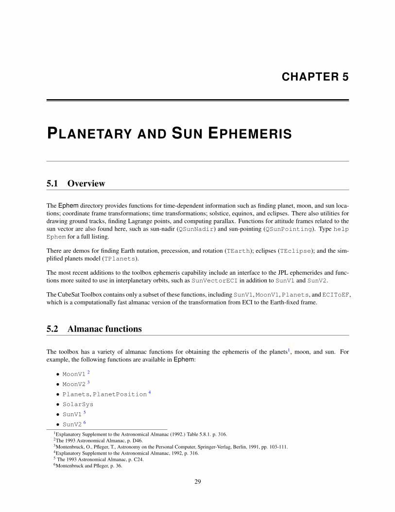
5 Ephemeris 295.1 Overview . . . . . . . . . . . . . . . . . . . . . . . . . . . . . . . . . . . . . . . . . . . . . . . . . 295.2 Almanac functions . . . . . . . . . . . . . . . . . . . . . . . . . . . . . . . . . . . . . . . . . . . . 295.3 JPL Ephemeris . . . . . . . . . . . . . . . . . . . . . . . . . . . . . . . . . . . . . . . . . . . . . . 30

6 CubeSat 336.1 CubeSat Modeling . . . . . . . . . . . . . . . . . . . . . . . . . . . . . . . . . . . . . . . . . . . . 346.2 Simulation . . . . . . . . . . . . . . . . . . . . . . . . . . . . . . . . . . . . . . . . . . . . . . . . . 366.3 Mission Planning . . . . . . . . . . . . . . . . . . . . . . . . . . . . . . . . . . . . . . . . . . . . . 39

iii

CONTENTS CONTENTS

6.4 Visualization . . . . . . . . . . . . . . . . . . . . . . . . . . . . . . . . . . . . . . . . . . . . . . . 406.5 Subsystems Modeling . . . . . . . . . . . . . . . . . . . . . . . . . . . . . . . . . . . . . . . . . . . 42

7 Coordinate Frames 437.1 Overview . . . . . . . . . . . . . . . . . . . . . . . . . . . . . . . . . . . . . . . . . . . . . . . . . 437.2 Orbital Element Sets . . . . . . . . . . . . . . . . . . . . . . . . . . . . . . . . . . . . . . . . . . . 447.3 Relative Coordinate Systems . . . . . . . . . . . . . . . . . . . . . . . . . . . . . . . . . . . . . . . 44

8 Relative Orbit Dynamics 498.1 Organization . . . . . . . . . . . . . . . . . . . . . . . . . . . . . . . . . . . . . . . . . . . . . . . . 498.2 Relative Dynamics in Circular Orbits . . . . . . . . . . . . . . . . . . . . . . . . . . . . . . . . . . . 498.3 Relative Dynamics in Eccentric Orbits . . . . . . . . . . . . . . . . . . . . . . . . . . . . . . . . . . 50

Index 55

CubeSat Toolbox iv

LIST OF FIGURES

2.1 MATLAB Help - Supplemental Software . . . . . . . . . . . . . . . . . . . . . . . . . . . . . . . . 42.2 Toolbox Documentation Main Page, R2016b . . . . . . . . . . . . . . . . . . . . . . . . . . . . . . . 52.3 Toolbox Documentation, R2011b . . . . . . . . . . . . . . . . . . . . . . . . . . . . . . . . . . . . . 52.4 Toolbox Demos . . . . . . . . . . . . . . . . . . . . . . . . . . . . . . . . . . . . . . . . . . . . . . 62.5 The file help GUI . . . . . . . . . . . . . . . . . . . . . . . . . . . . . . . . . . . . . . . . . . . . . 102.6 The demo GUI . . . . . . . . . . . . . . . . . . . . . . . . . . . . . . . . . . . . . . . . . . . . . . 132.7 On-line Help . . . . . . . . . . . . . . . . . . . . . . . . . . . . . . . . . . . . . . . . . . . . . . . 14

3.1 Atmospheric density from AtmDens2 . . . . . . . . . . . . . . . . . . . . . . . . . . . . . . . . . . 193.2 Elliptical orbit from RVFromKepler . . . . . . . . . . . . . . . . . . . . . . . . . . . . . . . . . . 203.3 A sine wave using Plot2D . . . . . . . . . . . . . . . . . . . . . . . . . . . . . . . . . . . . . . . . 23

4.1 Frames A and B . . . . . . . . . . . . . . . . . . . . . . . . . . . . . . . . . . . . . . . . . . . . . . 254.2 Selenographic to ECI frame . . . . . . . . . . . . . . . . . . . . . . . . . . . . . . . . . . . . . . . . 274.3 Areocentric frame . . . . . . . . . . . . . . . . . . . . . . . . . . . . . . . . . . . . . . . . . . . . . 28

5.1 Planet trajectories as generated by the built-in demo of SolarSysJPL . . . . . . . . . . . . . . . . 32

6.1 Model of 2U CubeSat . . . . . . . . . . . . . . . . . . . . . . . . . . . . . . . . . . . . . . . . . . . 356.2 Orbit simulation timestep results, simple on the left with with disturbances on the right. . . . . . . . . 376.3 Orbit evolution for an initial separation of 10 meters . . . . . . . . . . . . . . . . . . . . . . . . . . . 376.4 CubeSatSimulation example results . . . . . . . . . . . . . . . . . . . . . . . . . . . . . . . . 386.5 Observation time windows . . . . . . . . . . . . . . . . . . . . . . . . . . . . . . . . . . . . . . . . 396.6 RapidSwath built-in demo results . . . . . . . . . . . . . . . . . . . . . . . . . . . . . . . . . . . 406.7 Orbit visualization with PlotOrbit and GroundTrack . . . . . . . . . . . . . . . . . . . . . . . 406.8 CubeSat model with deployable solar panels viewed with DrawCubeSat . . . . . . . . . . . . . . . 416.9 Spacecraft visualization with sight lines using DrawSpacecraftInOrbit . . . . . . . . . . . . . 416.10 Playback demo using PlaybackOrbitSim . . . . . . . . . . . . . . . . . . . . . . . . . . . . . . 42

7.1 Relative Orbit Coordinate Frames . . . . . . . . . . . . . . . . . . . . . . . . . . . . . . . . . . . . 457.2 Geometric Parameters for Circular Orbits . . . . . . . . . . . . . . . . . . . . . . . . . . . . . . . . 467.3 Eccentric Parameters for Circular Orbits . . . . . . . . . . . . . . . . . . . . . . . . . . . . . . . . . 47

8.1 Results from FFEccFrameCompare Demo . . . . . . . . . . . . . . . . . . . . . . . . . . . . . . 52

v

LIST OF FIGURES LIST OF FIGURES

CubeSat Toolbox vi

CHAPTER 1

INTRODUCTION

This chapter shows you how to install the CubeSat Toolbox and how it is organized.

1.1 Organization

The CubeSat Toolbox is composed of MATLAB m-files and mat-files, organized into a set of modules by subject.It is essentially a library of functions for analyzing spacecraft and missions. The CubeSat toolbox is a subset ofthe Spacecraft Control Toolbox, which supports a set of scripts for analyzing mission planning, attitude control, andsimulation of nano satellites. The Spacecraft Control Toolbox is composed of a set of modules including CubeSat ,and that organization is preserved in the CubeSat Toolbox.

There is a substantial set of software which the Spacecraft Control Toolbox shares with the Aircraft Control Toolbox,and this software is in a module called Common. The core spacecraft analysis functions are in SC along with ananimation tool in Plotting. These modules with CubeSat are referred to together as the Core toolbox. All of theSpacecraft Control Toolbox modules are described in the following table, including the add-on modules which arepurchased separately.

Table 1.1: Spacecraft Control Toolbox ModulesModule FunctionCubeSat CubeSat and nanonsatellite modelingCommon Coordinate transformations, math, control, CAD tools, time conversions, graph-

ics and general utilitiesPlotting Plotting tools for complex simulations including animationSC Attitude dynamics, pointing budgets, basic orbit dynamics, environment, sample

CAD models, ephemeris, sensor and actuator modeling.SCPro Additional high-fidelity models for environment, sensors, actuators.AttitudeControl In-depth attitude control system design examples, including the hypothetical

geosynchronous satellite ComStarEstimation Attitude and orbit estimation. Stellar attitude determination and Kalman filtering.Imaging Image processing functionsLink Basic RF and optical link analysis.Orbit Orbit mechanics, maneuver planning, fuel budgets, and high-fidelity simulation.Power Basic power modelingPropulsion Electric and chemical propulsion. Launch vehicle analysis.Thermal Basic thermal modelingLaunch Vehicle Add-On Launch vehicle design

1

1.2. REQUIREMENTS CHAPTER 1. INTRODUCTION

Formation Flying Add-On Formation flying controlFusion Propulsion Add-On Fusion propulsion analysisSAAD Add-On Spin axis attitude determinationSolar Sail Add-On Solar sail control and mission analysis

The Formation Flying, Solar Sail, and SAAD add-on modules have their own user’s guides. These modules can bepurchased separately but they require the Professional Edition of the toolbox.

1.2 Requirements

MATLAB 7.0 at a minimum is required to run all of the functions. Most of the functions will run on previous versionsbut we are no longer supporting them.

1.3 Installation

The preferred method of delivering the toolbox is a download from the Princeton Satellite Systems website. Put thefolder extracted from the archive anywhere on your computer. There is no “installer” application to do the copying foryou. We will refer to the folder containing your modules as PSSToolboxes. If you later purchase an add-on module,you would simply add it to this folder.

All you need to do now is to set the MATLAB path to include the folders in PSSToolboxes. We recommend usingthe supplied function PSSSetPaths.m instead of MATLAB’s path utility. From the MATLAB prompt, cd to yourPSSToolboxes folder and then run PSSSetPaths. For example:

>> cd /Users/me/PSSToolboxes>> PSSSetPaths

This will set all of the paths for the duration of the session, with the option of saving the new path for future sessions.

1.4 Getting Started

The first two functions that you should try are DemoPSS and FileHelp. Each toolbox or module has a Demosfolder and a function DemoPSS. Do not move or remove this function from any of your modules! DemoPSS.m looksfor other DemoPSS functions to determine where the demos are in the folders so it can display them in the DemoPSSGUI.

The FileHelp function provides a graphical interface to the MATLAB function headers. You can peruse the functionsby folder to get a quick sense of your new product’s capabilities and search the function names and headers forkeywords. FileHelp and DemoPSS provide the best way to get an overview of the Spacecraft Control Toolbox.Both are described in more detail in the next chapter.

Demos and Functions can also be browsed by MATLAB’s built-in help system. sThis allows for the same searchingand browsing capabilities as DemoPSS and FileHelp.

CubeSat Toolbox 2

CHAPTER 2

GETTING HELP

This chapter shows you how to use the help systems built into PSS Toolboxes. There are several sources of help.Our toolboxes are now integrated into MATLAB’s built-in help browser. Then, there is the MATLAB command linehelp which prints help comments for individual files and lists the contents of folders. Then, there are special helputilities built into the PSS toolboxes: one is the file help function, the second is the demo functions and the thirdis the graphical user interface help system. Additionally, you can submit technical support questions directly to ourengineers via email.

2.1 MATLAB’s Built-in Help System

2.1.1 Basic Information and Function Help

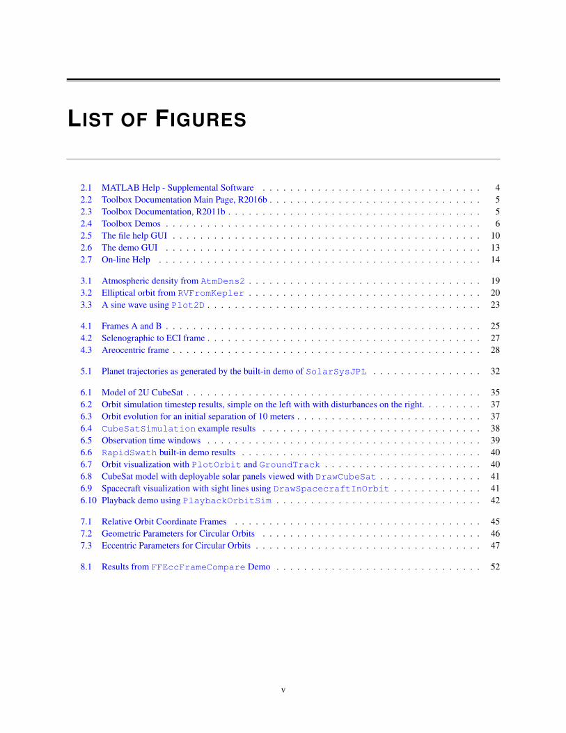
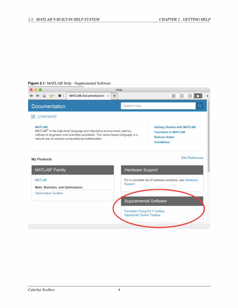
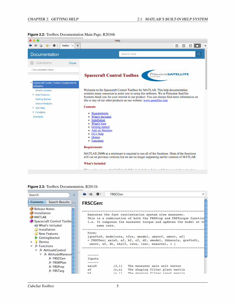
Our toolbox information can now be found in the MATLAB help system. To access this capability, simply open theMATLAB help system. As long as the toolbox is in the MATLAB path, it will appear in the contents pane. In morerecent versions of MATLAB, you need to navigate to Supplemental Software from the main window, as shown inFigure 2.1 on the following page. The index page of the SCT documentation is shown in Figure 2.2 on page 5.

The help window from R2011b and earlier is depicted in Figure 2.3 on page 5.

This contains a lot information on the toolbox. It also allows you to search for functions as you would if you weresearching for functions in the MATLAB root.

2.1.2 Published Demos

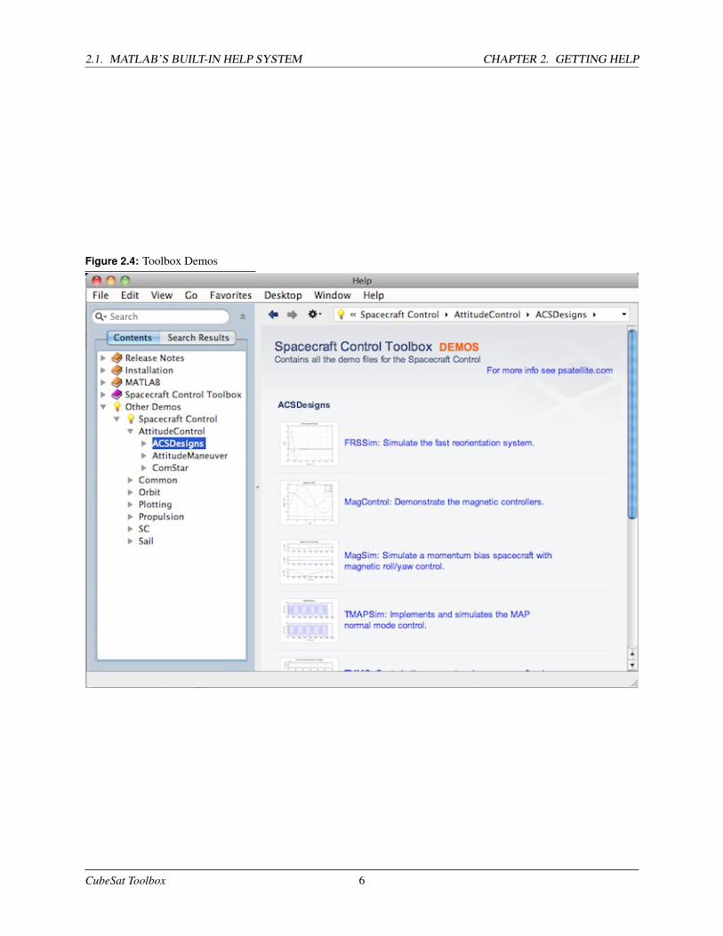
Another feature that has been added to the MATLAB help structure is the access to all of the toolbox demos. Everysingle demo is now listed, according to module and the folder. These can be found under the Other Demos or Examplesportion of the Contents Pane. Each demo has its own webpage that goes through it step by step showing exactly whatthe script is doing and which functions it is calling. From each individual demo webpage you can also run the scriptto view the output, or open it in the editor. Note that you might want to save any changes to the demo under a new filename so that you can always have the original. Below is an example of demo page displayed in MATLAB help thatshows where to find the toolbox demos as well as the the hierarchal structure used for browsing the demos.

3

2.1. MATLAB’S BUILT-IN HELP SYSTEM CHAPTER 2. GETTING HELP

Figure 2.1: MATLAB Help - Supplemental Software

CubeSat Toolbox 4

CHAPTER 2. GETTING HELP 2.1. MATLAB’S BUILT-IN HELP SYSTEM

Figure 2.2: Toolbox Documentation Main Page, R2016b

Figure 2.3: Toolbox Documentation, R2011b

CubeSat Toolbox 5

2.1. MATLAB’S BUILT-IN HELP SYSTEM CHAPTER 2. GETTING HELP

Figure 2.4: Toolbox Demos

CubeSat Toolbox 6

CHAPTER 2. GETTING HELP 2.2. COMMAND LINE HELP

2.2 Command Line Help

You can get help for any function by typing

>> help functionName

For example, if you type

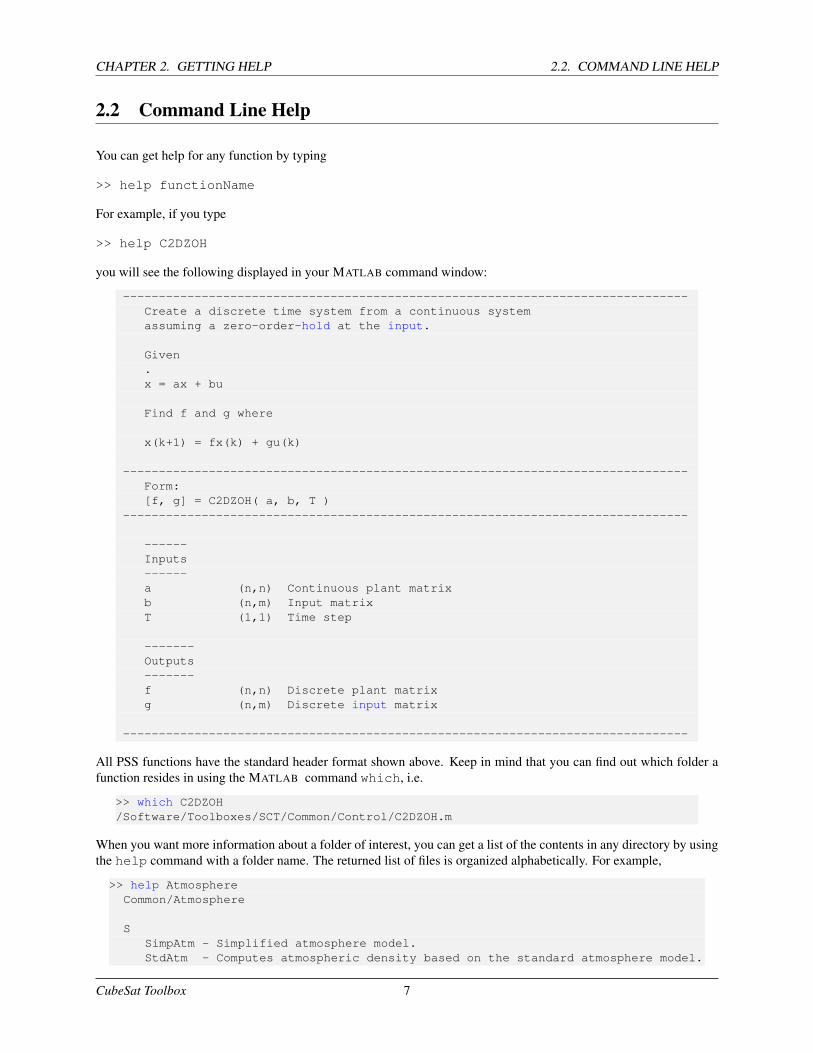
>> help C2DZOH

you will see the following displayed in your MATLAB command window:

-------------------------------------------------------------------------------Create a discrete time system from a continuous systemassuming a zero-order-hold at the input.

Given.x = ax + bu

Find f and g where

x(k+1) = fx(k) + gu(k)

-------------------------------------------------------------------------------Form:[f, g] = C2DZOH( a, b, T )

-------------------------------------------------------------------------------

------Inputs------a (n,n) Continuous plant matrixb (n,m) Input matrixT (1,1) Time step

-------Outputs-------f (n,n) Discrete plant matrixg (n,m) Discrete input matrix

-------------------------------------------------------------------------------

All PSS functions have the standard header format shown above. Keep in mind that you can find out which folder afunction resides in using the MATLAB command which, i.e.

>> which C2DZOH/Software/Toolboxes/SCT/Common/Control/C2DZOH.m

When you want more information about a folder of interest, you can get a list of the contents in any directory by usingthe help command with a folder name. The returned list of files is organized alphabetically. For example,

>> help AtmosphereCommon/Atmosphere

SSimpAtm - Simplified atmosphere model.StdAtm - Computes atmospheric density based on the standard atmosphere model.

CubeSat Toolbox 7

2.2. COMMAND LINE HELP CHAPTER 2. GETTING HELP

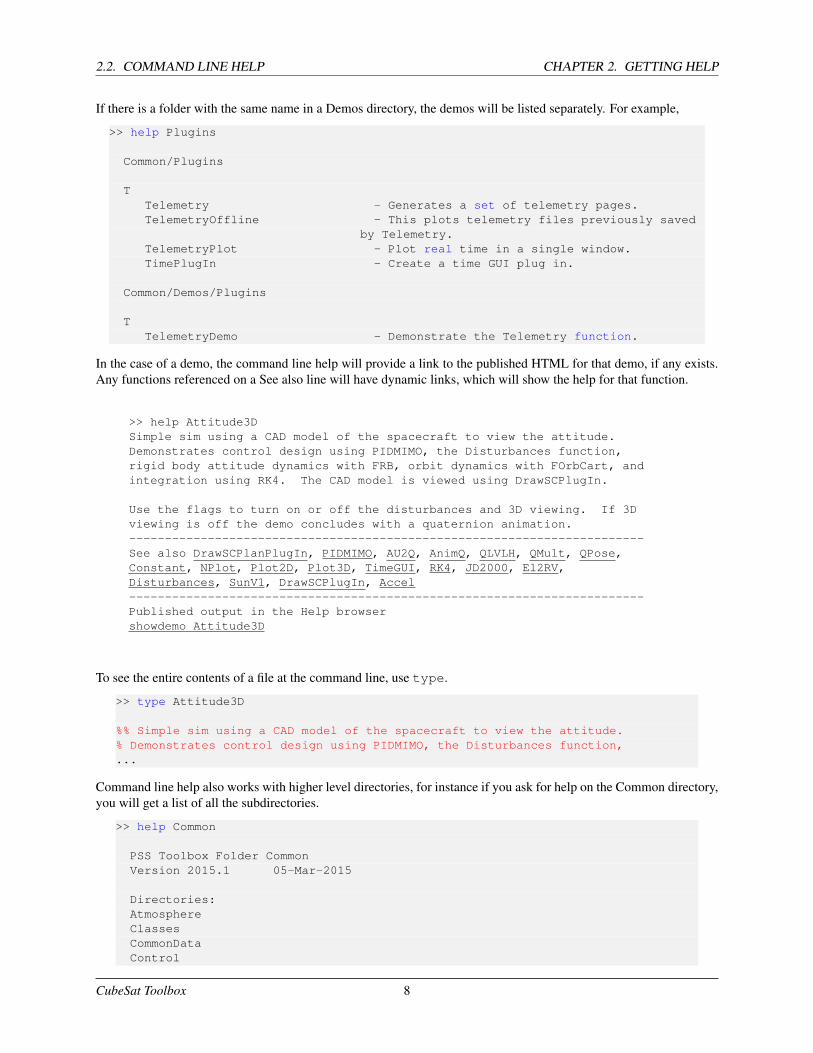
If there is a folder with the same name in a Demos directory, the demos will be listed separately. For example,

>> help Plugins

Common/Plugins

TTelemetry - Generates a set of telemetry pages.TelemetryOffline - This plots telemetry files previously saved

by Telemetry.TelemetryPlot - Plot real time in a single window.TimePlugIn - Create a time GUI plug in.

Common/Demos/Plugins

TTelemetryDemo - Demonstrate the Telemetry function.

In the case of a demo, the command line help will provide a link to the published HTML for that demo, if any exists.Any functions referenced on a See also line will have dynamic links, which will show the help for that function.

>> help Attitude3DSimple sim using a CAD model of the spacecraft to view the attitude.Demonstrates control design using PIDMIMO, the Disturbances function,rigid body attitude dynamics with FRB, orbit dynamics with FOrbCart, andintegration using RK4. The CAD model is viewed using DrawSCPlugIn.

Use the flags to turn on or off the disturbances and 3D viewing. If 3Dviewing is off the demo concludes with a quaternion animation.------------------------------------------------------------------------See also DrawSCPlanPlugIn, PIDMIMO, AU2Q, AnimQ, QLVLH, QMult, QPose,Constant, NPlot, Plot2D, Plot3D, TimeGUI, RK4, JD2000, El2RV,Disturbances, SunV1, DrawSCPlugIn, Accel------------------------------------------------------------------------Published output in the Help browsershowdemo Attitude3D

To see the entire contents of a file at the command line, use type.

>> type Attitude3D

%% Simple sim using a CAD model of the spacecraft to view the attitude.% Demonstrates control design using PIDMIMO, the Disturbances function,...

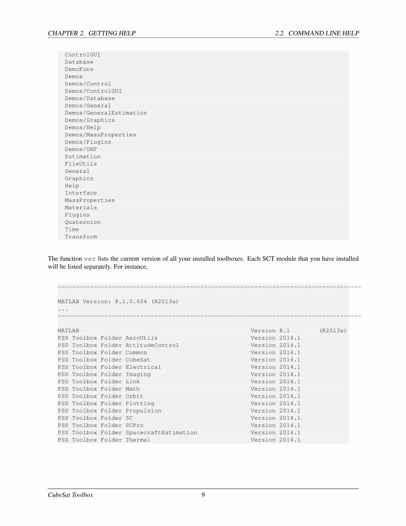
Command line help also works with higher level directories, for instance if you ask for help on the Common directory,you will get a list of all the subdirectories.

>> help Common

PSS Toolbox Folder CommonVersion 2015.1 05-Mar-2015

Directories:AtmosphereClassesCommonDataControl

CubeSat Toolbox 8

CHAPTER 2. GETTING HELP 2.2. COMMAND LINE HELP

ControlGUIDatabaseDemoFunsDemosDemos/ControlDemos/ControlGUIDemos/DatabaseDemos/GeneralDemos/GeneralEstimationDemos/GraphicsDemos/HelpDemos/MassPropertiesDemos/PluginsDemos/UKFEstimationFileUtilsGeneralGraphicsHelpInterfaceMassPropertiesMaterialsPluginsQuaternionTimeTransform

The function ver lists the current version of all your installed toolboxes. Each SCT module that you have installedwill be listed separately. For instance,

-------------------------------------------------------------------------------------

MATLAB Version: 8.1.0.604 (R2013a)...-------------------------------------------------------------------------------------

MATLAB Version 8.1 (R2013a)PSS Toolbox Folder AeroUtils Version 2014.1PSS Toolbox Folder AttitudeControl Version 2014.1PSS Toolbox Folder Common Version 2014.1PSS Toolbox Folder CubeSat Version 2014.1PSS Toolbox Folder Electrical Version 2014.1PSS Toolbox Folder Imaging Version 2014.1PSS Toolbox Folder Link Version 2014.1PSS Toolbox Folder Math Version 2014.1PSS Toolbox Folder Orbit Version 2014.1PSS Toolbox Folder Plotting Version 2014.1PSS Toolbox Folder Propulsion Version 2014.1PSS Toolbox Folder SC Version 2014.1PSS Toolbox Folder SCPro Version 2014.1PSS Toolbox Folder SpacecraftEstimation Version 2014.1PSS Toolbox Folder Thermal Version 2014.1

CubeSat Toolbox 9

2.3. FILEHELP CHAPTER 2. GETTING HELP

2.3 FileHelp

2.3.1 Introduction

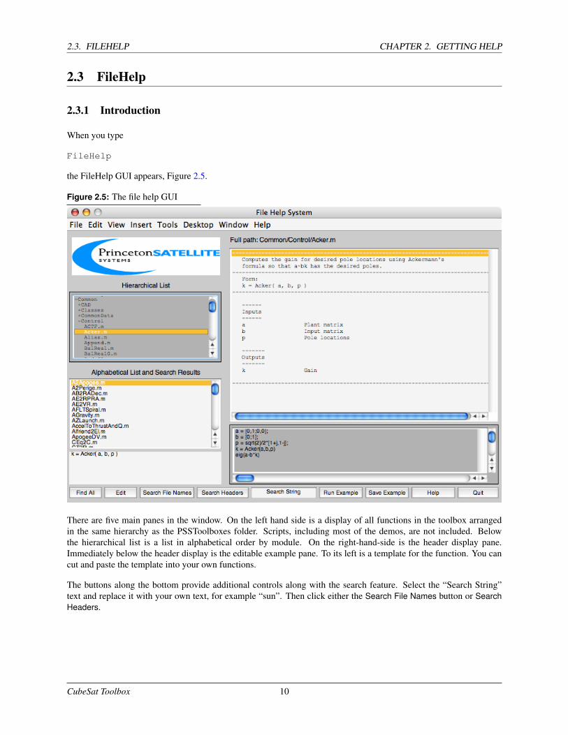
When you type

FileHelp

the FileHelp GUI appears, Figure 2.5.

Figure 2.5: The file help GUI

There are five main panes in the window. On the left hand side is a display of all functions in the toolbox arrangedin the same hierarchy as the PSSToolboxes folder. Scripts, including most of the demos, are not included. Belowthe hierarchical list is a list in alphabetical order by module. On the right-hand-side is the header display pane.Immediately below the header display is the editable example pane. To its left is a template for the function. You cancut and paste the template into your own functions.

The buttons along the bottom provide additional controls along with the search feature. Select the “Search String”text and replace it with your own text, for example “sun”. Then click either the Search File Names button or SearchHeaders.

CubeSat Toolbox 10

CHAPTER 2. GETTING HELP 2.4. SEARCHING IN FILE HELP

2.3.2 The List Pane

If you click a file in the alphabetical or hierarchical lists, the header will appear in the header pane. This is the sameheader that is in the file. The headers are extracted from a .mat file so changes you make will not be reflected in thefile. In the hierarchical list, any name with a + or - sign is a folder. Click on the folders until you reach the file youwould like. When you click a file, the header and template will appear.

2.3.3 Edit Button

This opens the MATLAB edit window for the function selected in the list.

2.3.4 The Example Pane

This pane gives an example for the function displayed. Not all functions have examples. The edit display has scrollbars. You can edit the example, create new examples and save them using the buttons below the display. To run anexample, push the Run Example button. You can include comments in the example by using the percent symbol.

2.3.5 Run Example Button

Run the example in the display. Some of the examples are just the name of the function. These are functions withbuilt-in demos. Results will appear either in separate figure windows or in the MATLAB Command Window.

2.3.6 Save Example Button

Save the example in the edit window. Pushing this button only saves it in the temporary memory used by the GUI.You can save the example permanently when you Quit.

2.3.7 Help Button

Opens the on-line help system.

2.3.8 Quit

Quit the GUI. If you have edited an example, it will ask you whether you want to save the example before you quit.

2.4 Searching in File Help

2.4.1 Search File Names Button

Type in a function name in the edit box and push the button called Search File Names.

2.4.2 Find All Button

Find All returns to the original list of the functions. This is used after one of the search options has been used.

CubeSat Toolbox 11

2.5. FINDER CHAPTER 2. GETTING HELP

2.4.3 Search Headers Button

Search headers for a string. This function looks for exact, but not case sensitive, matches. The file display displays allmatches. A progress bar gives you an indication of time remaining in the search.

2.4.4 Search String Edit Box

This is the search string. Spaces will be matched so if you type attitude control it will not match attitude control (withtwo spaces.)

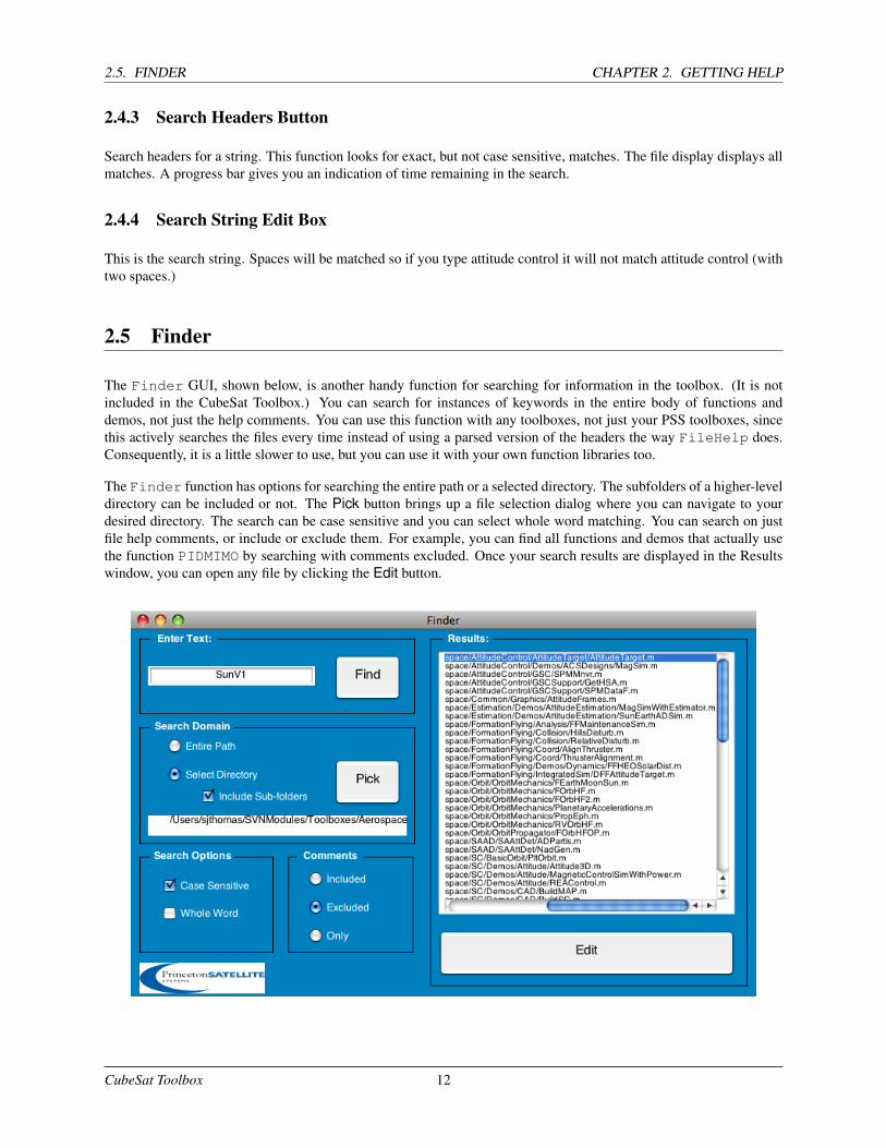
2.5 Finder

The Finder GUI, shown below, is another handy function for searching for information in the toolbox. (It is notincluded in the CubeSat Toolbox.) You can search for instances of keywords in the entire body of functions anddemos, not just the help comments. You can use this function with any toolboxes, not just your PSS toolboxes, sincethis actively searches the files every time instead of using a parsed version of the headers the way FileHelp does.Consequently, it is a little slower to use, but you can use it with your own function libraries too.

The Finder function has options for searching the entire path or a selected directory. The subfolders of a higher-leveldirectory can be included or not. The Pick button brings up a file selection dialog where you can navigate to yourdesired directory. The search can be case sensitive and you can select whole word matching. You can search on justfile help comments, or include or exclude them. For example, you can find all functions and demos that actually usethe function PIDMIMO by searching with comments excluded. Once your search results are displayed in the Resultswindow, you can open any file by clicking the Edit button.

CubeSat Toolbox 12

CHAPTER 2. GETTING HELP 2.6. DEMOPSS

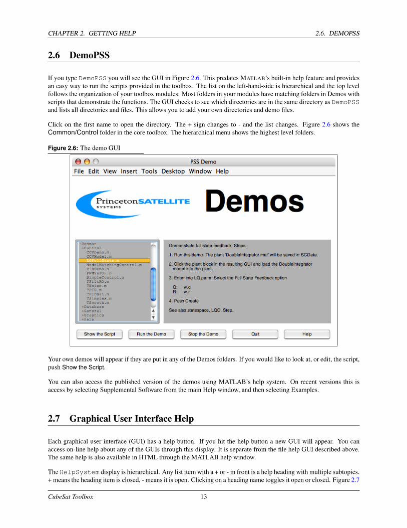
2.6 DemoPSS

If you type DemoPSS you will see the GUI in Figure 2.6. This predates MATLAB’s built-in help feature and providesan easy way to run the scripts provided in the toolbox. The list on the left-hand-side is hierarchical and the top levelfollows the organization of your toolbox modules. Most folders in your modules have matching folders in Demos withscripts that demonstrate the functions. The GUI checks to see which directories are in the same directory as DemoPSSand lists all directories and files. This allows you to add your own directories and demo files.

Click on the first name to open the directory. The + sign changes to - and the list changes. Figure 2.6 shows theCommon/Control folder in the core toolbox. The hierarchical menu shows the highest level folders.

Figure 2.6: The demo GUI

Your own demos will appear if they are put in any of the Demos folders. If you would like to look at, or edit, the script,push Show the Script.

You can also access the published version of the demos using MATLAB’s help system. On recent versions this isaccess by selecting Supplemental Software from the main Help window, and then selecting Examples.

2.7 Graphical User Interface Help

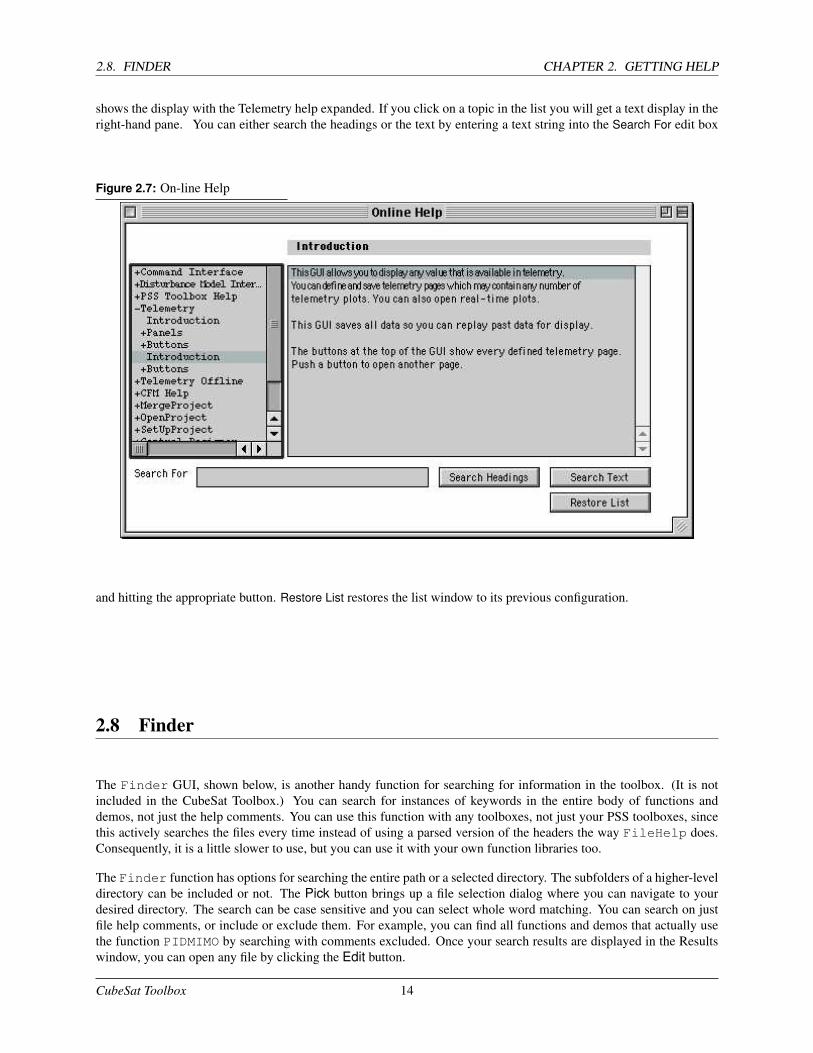
Each graphical user interface (GUI) has a help button. If you hit the help button a new GUI will appear. You canaccess on-line help about any of the GUIs through this display. It is separate from the file help GUI described above.The same help is also available in HTML through the MATLAB help window.

The HelpSystem display is hierarchical. Any list item with a + or - in front is a help heading with multiple subtopics.+ means the heading item is closed, - means it is open. Clicking on a heading name toggles it open or closed. Figure 2.7

CubeSat Toolbox 13

2.8. FINDER CHAPTER 2. GETTING HELP

shows the display with the Telemetry help expanded. If you click on a topic in the list you will get a text display in theright-hand pane. You can either search the headings or the text by entering a text string into the Search For edit box

Figure 2.7: On-line Help

and hitting the appropriate button. Restore List restores the list window to its previous configuration.

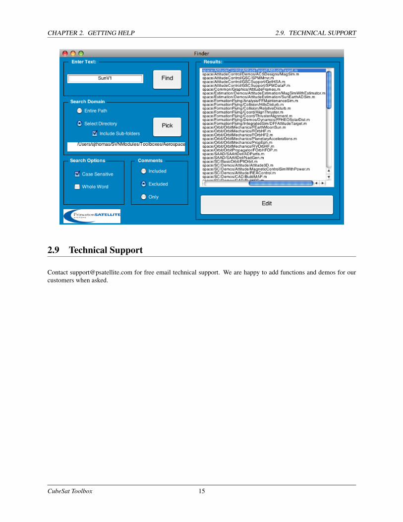
2.8 Finder

The Finder GUI, shown below, is another handy function for searching for information in the toolbox. (It is notincluded in the CubeSat Toolbox.) You can search for instances of keywords in the entire body of functions anddemos, not just the help comments. You can use this function with any toolboxes, not just your PSS toolboxes, sincethis actively searches the files every time instead of using a parsed version of the headers the way FileHelp does.Consequently, it is a little slower to use, but you can use it with your own function libraries too.

The Finder function has options for searching the entire path or a selected directory. The subfolders of a higher-leveldirectory can be included or not. The Pick button brings up a file selection dialog where you can navigate to yourdesired directory. The search can be case sensitive and you can select whole word matching. You can search on justfile help comments, or include or exclude them. For example, you can find all functions and demos that actually usethe function PIDMIMO by searching with comments excluded. Once your search results are displayed in the Resultswindow, you can open any file by clicking the Edit button.

CubeSat Toolbox 14

CHAPTER 2. GETTING HELP 2.9. TECHNICAL SUPPORT

2.9 Technical Support

Contact support@psatellite.com for free email technical support. We are happy to add functions and demos for ourcustomers when asked.

CubeSat Toolbox 15

2.9. TECHNICAL SUPPORT CHAPTER 2. GETTING HELP

CubeSat Toolbox 16

CHAPTER 3

BASIC FUNCTIONS

This chapter shows you how to use a sampling of the most basic Spacecraft Control Toolbox functions.

3.1 Introduction

The Spacecraft Control Toolbox is composed of several thousand MATLAB files. The functions cover attitude controland dynamics, computer aided design, orbit dynamics and kinematics, ephemeris, actuator and sensor modeling, andthermal and mathematics operations. Most of the functions can be used individually although some are rarely calledexcept by other toolbox functions.

This chapter will review some basic features built into the SCT functions and highlight some examples from the folderthat you will use most frequently.

3.2 Function Features

3.2.1 Introduction

Functions have several features that are helpful to understand. Features that are available in the functions are listed inTable 3.1.

Table 3.1: Features in Spacecraft Control Toolbox functions

FeaturesBuilt-in demosDefault parametersBuilt-in plottingError checkingVariable inputs

These are illustrated in the examples given below.

17

3.2. FUNCTION FEATURES CHAPTER 3. BASIC FUNCTIONS

3.2.2 Built-in demos

Many functions have built in demos. A function with a built-in demo requires no inputs and produces a plot or otheroutput for a range of input parameters to give you a feel for the function.

An example of a function with a built-in demo is AnimQ. It creates an example array of quaternions and animates theresulting body axes. The inputs for the built-in demo are generally specified near the top of the function so it is easyto check for one by looking at the code. Plots are produced at the bottom of a function.

3.2.3 Default parameters

Most functions have default parameters. There are two ways to get default parameters. If you pass an empty matrix,i.e.

[]

as a parameter the function will use a default parameter if defaults are available. This is only necessary if you wish touse a default for one parameter and input the value for the next input. For example, EarthRot takes a date in Juliancenturies as the first parameter and a flag for equation of the equinoxes as the second parameter. If you look in thefunction, you will see that the default is to use the current date.

>> g = EarthRot( [], 1 )

g =-0.9815 -0.1914 00.1914 -0.9815 0

0 0 1.0000

The second way to get defaults is simply to leave off arguments at the end of the input list. For EarthRot the secondparameter is also optional.

>> g = EarthRot( )

g =-0.9815 -0.1916 00.1916 -0.9815 0

0 0 1.0000

You should never hesitate to look in functions to see what defaults are available and what the values are. Defaultsare always treated at the top of the function just under the header. Remember that the unix command type works inMATLAB to display a function’s contents, for instance

>> type EarthRot

function [g, gMST, gAST] = EarthRot( T, eOfECalc )

%-------------------------------------------------------------------------------% Computes the earth greenwich matrix that transforms from ECI to earth fixed.%-------------------------------------------------------------------------------% Form:% [g, gMST, gAST] = EarthRot( T, eOfECalc )%-------------------------------------------------------------------------------

...if( nargin < 1 )

T = [];end

CubeSat Toolbox 18

CHAPTER 3. BASIC FUNCTIONS 3.2. FUNCTION FEATURES

if( isempty( T ) )T = JD2T(Date2JD);

end

where we have excerpted the code creating the default input.

3.2.4 Built-in plotting

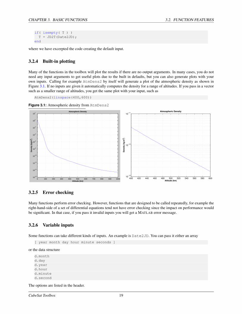
Many of the functions in the toolbox will plot the results if there are no output arguments. In many cases, you do notneed any input arguments to get useful plots due to the built in defaults, but you can also generate plots with yourown inputs. Calling for example AtmDens2 by itself will generate a plot of the atmospheric density as shown inFigure 3.1. If no inputs are given it automatically computes the density for a range of altitudes. If you pass in a vectorsuch as a smaller range of altitudes, you get the same plot with your input, such as

AtmDens2(linspace(400,600))

Figure 3.1: Atmospheric density from AtmDens2

0 100 200 300 400 500 600 700 800 900 100010

-16

10-14

10-12

10-10

10-8

10-6

10-4

10-2

100

102

Altitude (km)

Den

sity

(kg

/m3 )

Atmospheric Density

400 420 440 460 480 500 520 540 560 580 60010

−13

10−12

10−11

Altitude (km)

Den

sit

y (

kg

/m3)

Atmospheric Density

3.2.5 Error checking

Many functions perform error checking. However, functions that are designed to be called repeatedly, for example theright-hand-side of a set of differential equations tend not have error checking since the impact on performance wouldbe significant. In that case, if you pass it invalid inputs you will get a MATLAB error message.

3.2.6 Variable inputs

Some functions can take different kinds of inputs. An example is Date2JD. You can pass it either an array

[ year month day hour minute seconds ]

or the data structure

d.monthd.dayd.yeard.hourd.minuted.second

The options are listed in the header.

CubeSat Toolbox 19

3.3. EXAMPLE FUNCTIONS CHAPTER 3. BASIC FUNCTIONS

3.3 Example Functions

The following sections gives examples for selected functions from the major folders of the SCT core toolbox.

3.3.1 Basic Orbit

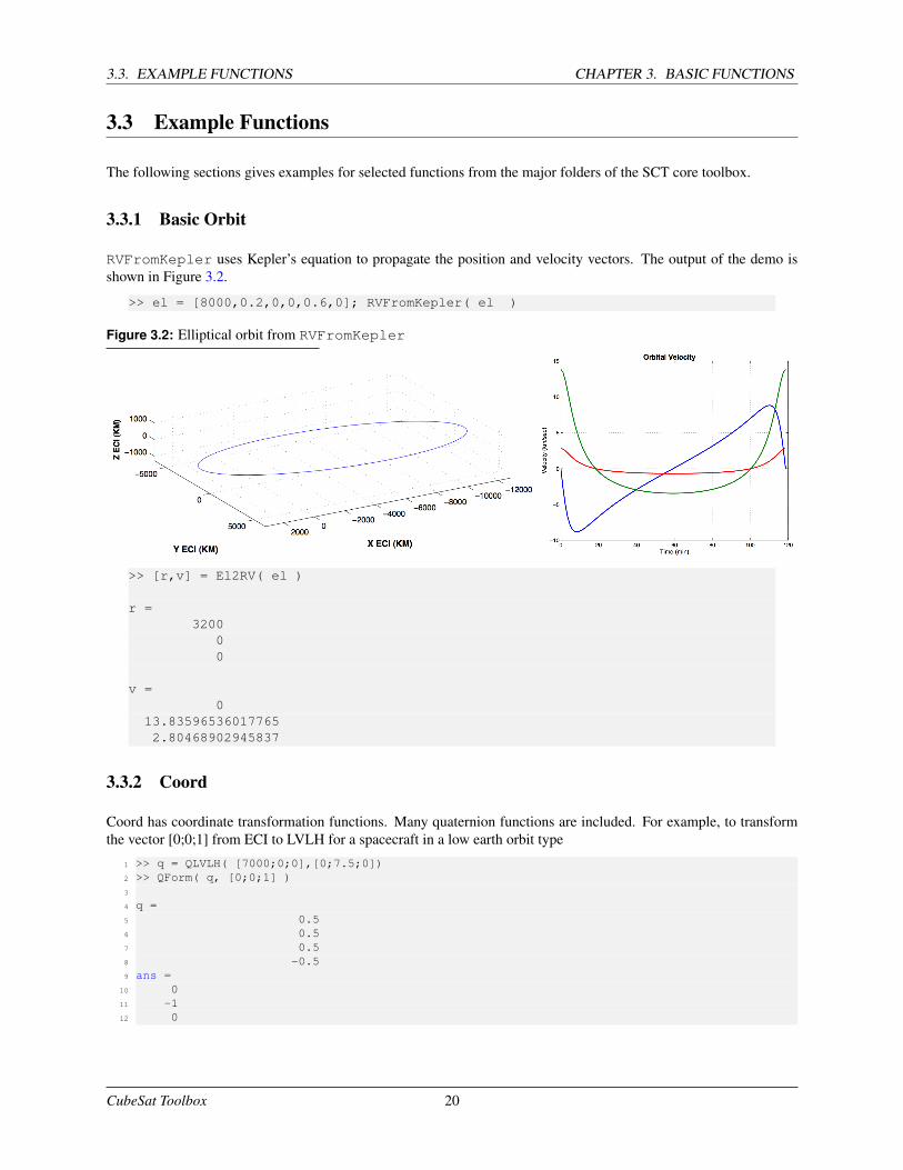
RVFromKepler uses Kepler’s equation to propagate the position and velocity vectors. The output of the demo isshown in Figure 3.2.

>> el = [8000,0.2,0,0,0.6,0]; RVFromKepler( el )

Figure 3.2: Elliptical orbit from RVFromKepler

>> [r,v] = El2RV( el )

r =3200

00

v =0

13.835965360177652.80468902945837

3.3.2 Coord

Coord has coordinate transformation functions. Many quaternion functions are included. For example, to transformthe vector [0;0;1] from ECI to LVLH for a spacecraft in a low earth orbit type

1 >> q = QLVLH( [7000;0;0],[0;7.5;0])2 >> QForm( q, [0;0;1] )3

4 q =5 0.56 0.57 0.58 -0.59 ans =

10 011 -112 0

CubeSat Toolbox 20

CHAPTER 3. BASIC FUNCTIONS 3.3. EXAMPLE FUNCTIONS

3.3.3 CAD

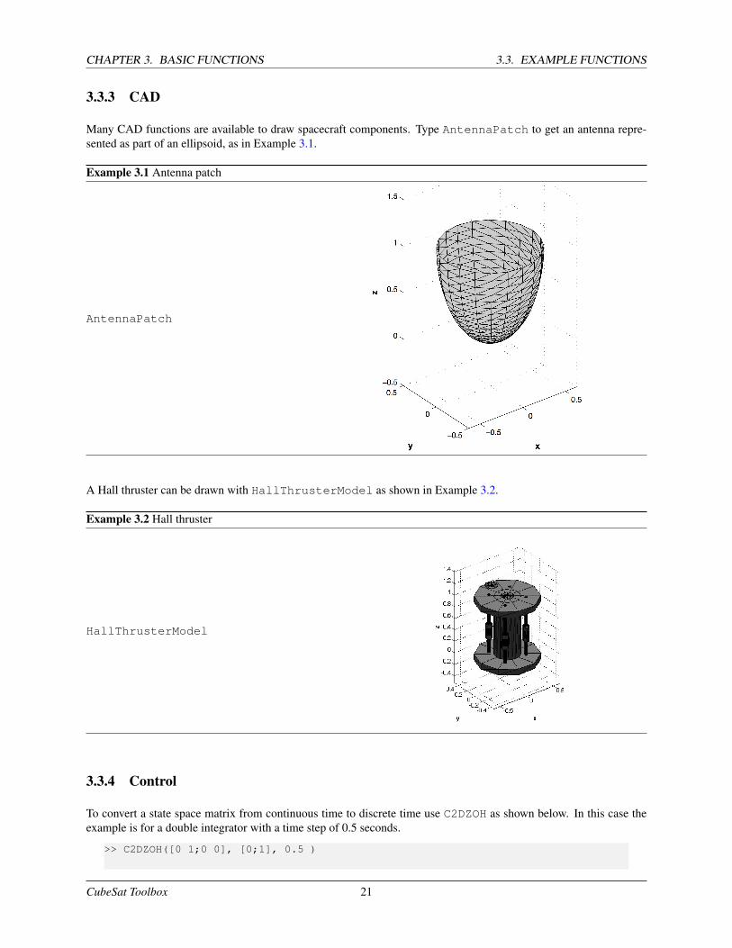
Many CAD functions are available to draw spacecraft components. Type AntennaPatch to get an antenna repre-sented as part of an ellipsoid, as in Example 3.1.

Example 3.1 Antenna patch

AntennaPatch

A Hall thruster can be drawn with HallThrusterModel as shown in Example 3.2.

Example 3.2 Hall thruster

HallThrusterModel

3.3.4 Control

To convert a state space matrix from continuous time to discrete time use C2DZOH as shown below. In this case theexample is for a double integrator with a time step of 0.5 seconds.

>> C2DZOH([0 1;0 0], [0;1], 0.5 )

CubeSat Toolbox 21

3.3. EXAMPLE FUNCTIONS CHAPTER 3. BASIC FUNCTIONS

ans =1 0.50 1

3.3.5 Dynamics

This function can return either a state-space system or the state derivative vector. RBModel has analytical expressionsfor the state space system of a rigid body spacecraft.

>> [a, b, c, d] = RBModel( diag([ 2 2 1]),[0;7.291e-5;0]);>> eig(a)

The resulting plant has a double integrator for each axis.

ans =000

3.3.6 Environs

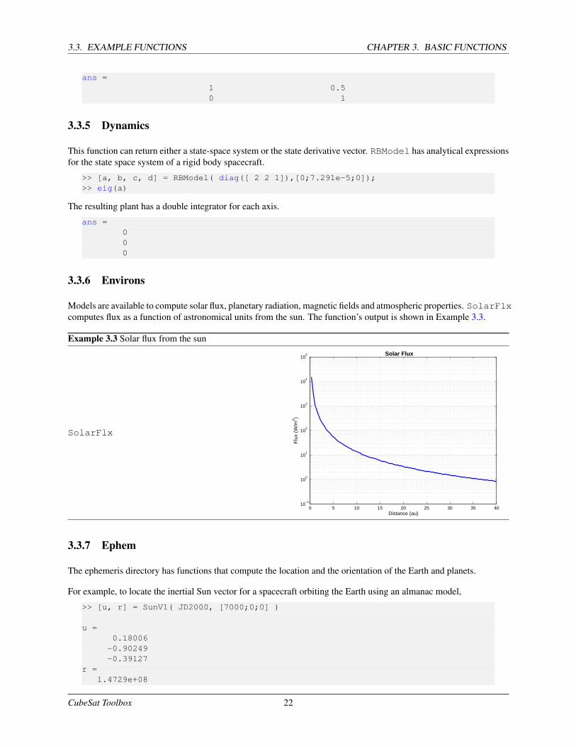
Models are available to compute solar flux, planetary radiation, magnetic fields and atmospheric properties. SolarFlxcomputes flux as a function of astronomical units from the sun. The function’s output is shown in Example 3.3.

Example 3.3 Solar flux from the sun

SolarFlx

Solar Flux

0 5 10 15 20 25 30 35 4010

−1

100

101

102

103

104

105

Flu

x (W

/m2 )

Distance (au)

3.3.7 Ephem

The ephemeris directory has functions that compute the location and the orientation of the Earth and planets.

For example, to locate the inertial Sun vector for a spacecraft orbiting the Earth using an almanac model,

>> [u, r] = SunV1( JD2000, [7000;0;0] )

u =0.18006

-0.90249-0.39127

r =1.4729e+08

CubeSat Toolbox 22

CHAPTER 3. BASIC FUNCTIONS 3.3. EXAMPLE FUNCTIONS

which returns a unit vector to the sun from the spacecraft and the distance from the origin to the sun. SunV2 providesthe same inputs and outputs and uses a higher precision sun model.

3.3.8 Graphics

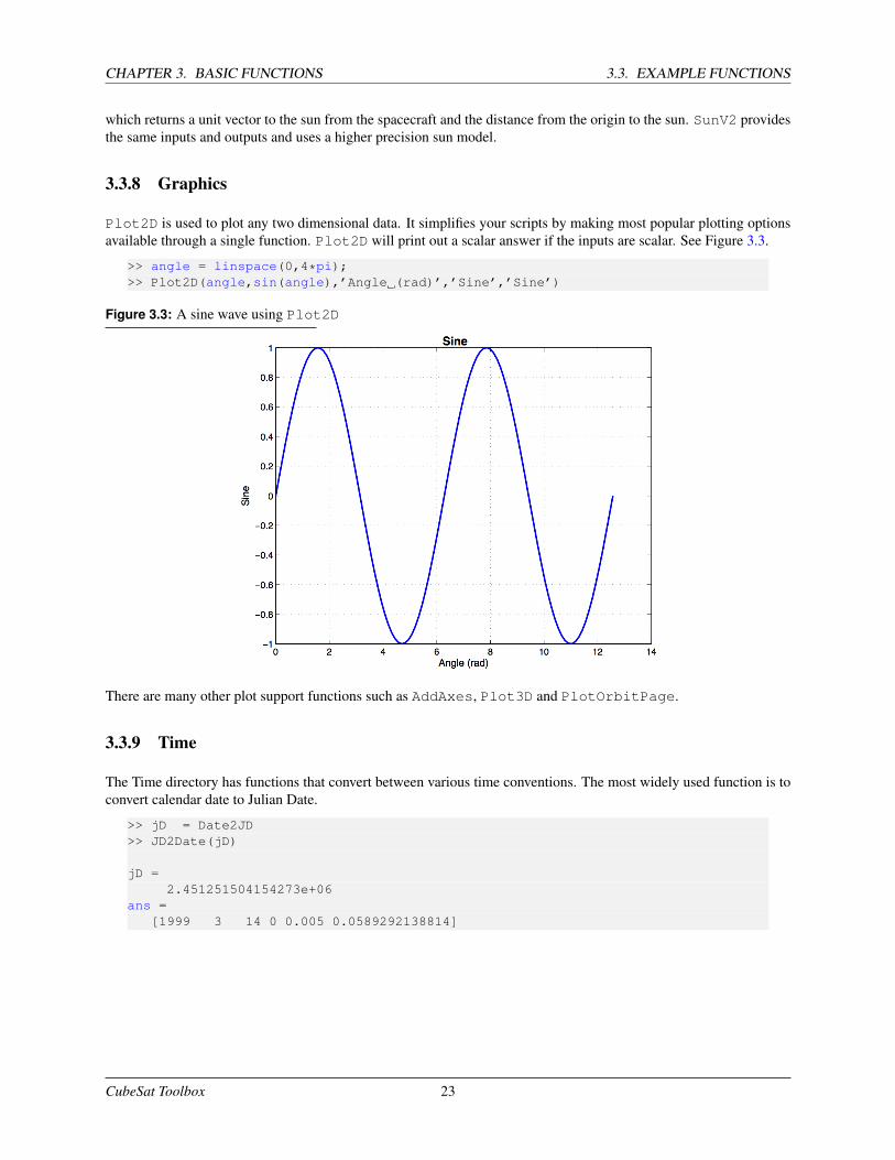
Plot2D is used to plot any two dimensional data. It simplifies your scripts by making most popular plotting optionsavailable through a single function. Plot2D will print out a scalar answer if the inputs are scalar. See Figure 3.3.

>> angle = linspace(0,4*pi);>> Plot2D(angle,sin(angle),’Angle (rad)’,’Sine’,’Sine’)

Figure 3.3: A sine wave using Plot2D

There are many other plot support functions such as AddAxes, Plot3D and PlotOrbitPage.

3.3.9 Time

The Time directory has functions that convert between various time conventions. The most widely used function is toconvert calendar date to Julian Date.

>> jD = Date2JD>> JD2Date(jD)

jD =2.451251504154273e+06

ans =[1999 3 14 0 0.005 0.0589292138814]

CubeSat Toolbox 23

3.3. EXAMPLE FUNCTIONS CHAPTER 3. BASIC FUNCTIONS

CubeSat Toolbox 24

CHAPTER 4

COORDINATE TRANSFORMATIONS

This chapter shows you how to use Spacecraft Control Toolbox functions for coordinate transformations. Thereis a very extensive set of functions in the Common/Coord folder covering quaternions, Euler angles, transformationmatrices, right ascension/declination, spherical coordinates, geodetic coordinates, and more. A few are discussed here.For more information on coordinate frames and representations, please see the Coordinate Systems and Kinematicschapters in the accompanying book Spacecraft Attitude and Orbit Control.

4.1 Transformation Matrices

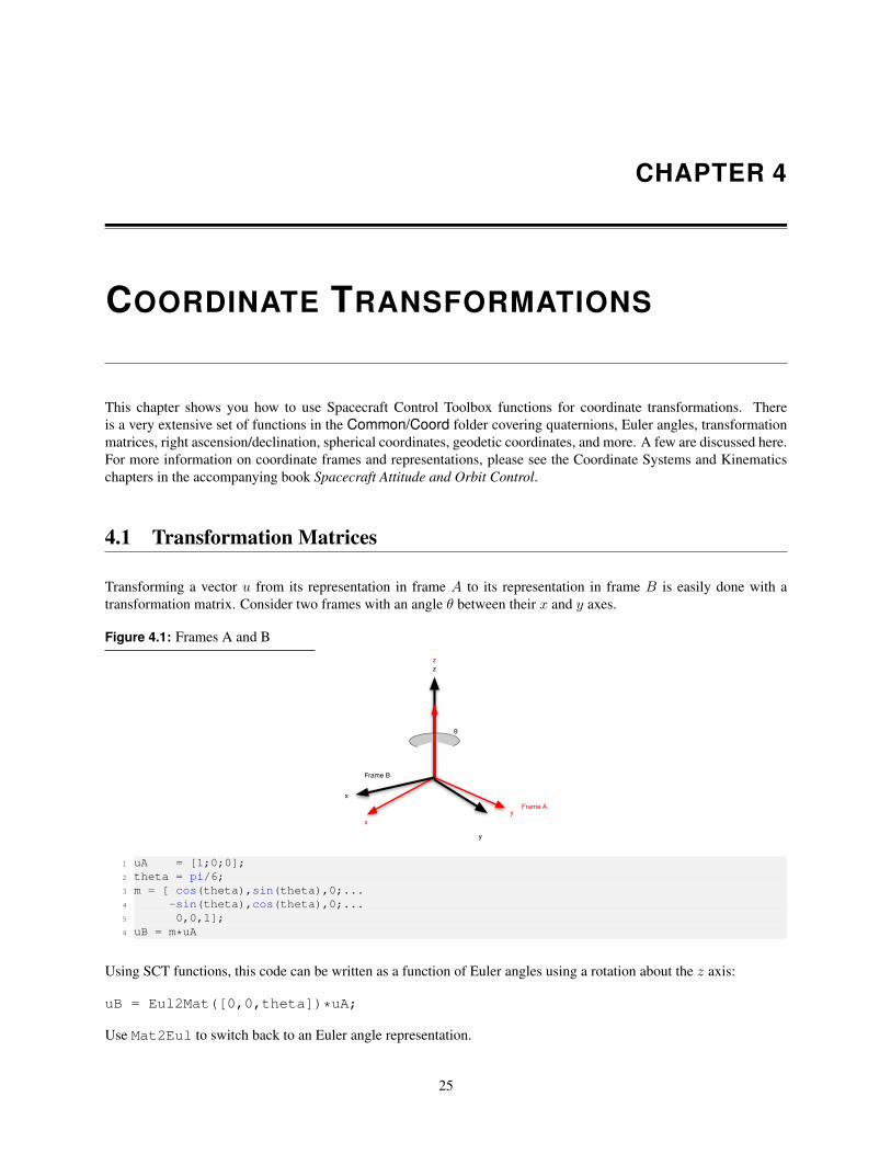
Transforming a vector u from its representation in frame A to its representation in frame B is easily done with atransformation matrix. Consider two frames with an angle θ between their x and y axes.

Figure 4.1: Frames A and B

z

x

y

z

yx

Frame A

Frame B

θ

1 uA = [1;0;0];2 theta = pi/6;3 m = [ cos(theta),sin(theta),0;...4 -sin(theta),cos(theta),0;...5 0,0,1];6 uB = m*uA

Using SCT functions, this code can be written as a function of Euler angles using a rotation about the z axis:

uB = Eul2Mat([0,0,theta])*uA;

Use Mat2Eul to switch back to an Euler angle representation.

25

4.2. QUATERNIONS CHAPTER 4. COORDINATES

4.2 Quaternions

A quaternion is a four parameter set that embodies the concept that any set of rotations can be represented by a singleaxis of rotation and an angle. PSS uses the shuttle convention so that our unit quaternion (obtained with QZero) is [10 0 0]. In Figure 4.1 on the preceding page the axis of rotation is [0 0 1] (the z axis) and the angle is theta. Ofcourse, the axis of rotation could also be [0 0 -1] and the angle -theta.

Quaternion transformations are implemented by the functions QForm and QTForm. QForm rotates a vector in thedirection of the quaternion, and QTForm rotates it in the opposite direction. In this case

q = Mat2Q(m);uB = QForm(q,uA)uA = QTForm(q,uB)

We could also get q by typing

q = Eul2Q([0;0;theta])

Much as you can concatenate coordinate transformation matrices, you can also multiply quaternions. If qAToBtransforms from A to B and qBToC transforms from B to C then

qAToC = QMult(qAToB,qBToC);

The transpose of a quaternion is just

qCToA = QPose(qAToC);

You can extract Euler angles by

eAToC = Q2Eul(qAToC);

or matrices by

mAToC = Q2Mat(qAToC);

If we convert the three Euler angles to a quaternion

qIToB = Eul2Q(e);

qIToB will transform vectors represented in I to vectors represented in B. This quaternion will be the transpose ofthe quaternion that rotates frame B from its initial orientation to its final orientation or

qIToB = QPose(qBInitialToBFinal);

Given a vector of small angles eSmall that rotate from vectors from frame A to B, the transformation from A to Bis

uB = (eye(3)-SkewSymm(eSmall))*uA;

where

SkewSymm([1;2;3])ans =[0 -3 2;3 0 -1;

-2 1 0]

Note that SkewSymm(x)*y is the same as Cross(x,y).

CubeSat Toolbox 26

CHAPTER 4. COORDINATES 4.3. COORDINATE FRAMES

4.3 Coordinate Frames

The toolbox has functions for many common coordinate frames and representations, including

• Earth-fixed frame, aerographic (Mars), selenographic (Moon)

• Latitude (geocentric and geodetic), longitude, and altitude

• Earth-centered inertial

• Local vertical, local horizontal

• Nadir and sun-nadir pointing

• Hills frame

• Rotating libration point

• Right ascension and declination

• Azimuth and elevation

• Spherical, cartesian, and cylindrical

Most of these functions can be found in Coord and some are in Ephem due to their dependence on ephemeris datasuch as the sun vector. A few relevant functions are in OrbitMechanics. For example, the QLVLH function in Coordcomputes a quaternion from the inertial to local-vertical local-horizontal frame from the position and velocity vectors.QNadirPoint, also in Coord, aligns a particular body vector with the nadir vector. The QSunNadir function inEphem computes the sun-nadir quaternion from the ECI spacecraft state and sun vector.

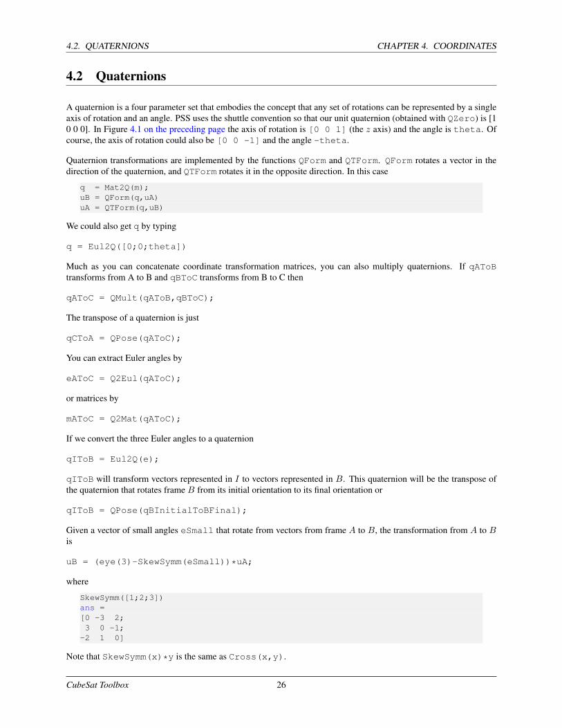
The relationship between the Selenographic and the ECI frame is computed by MoonRot and shown in Figure 4.2.φ′m is the Selenographic Latitude which is the acute angle measured normal to the Moon’s equator between the

Figure 4.2: Selenographic to ECI frame

equator and a line connecting the geometrical center of the coordinate system with a point on the surface of the Moon.The angle range is between 0 and 360 degrees. λm is the Selenographic Longitude which is the angle measuredtowards the West in the Moon’s equatorial plane, from the lunar prime meridian to the object’s meridian. The anglerange is between -90 and +90 degrees. North is the section above the lunar equator containing Mare Serenitatis. Westis measured towards Mare Crisium.

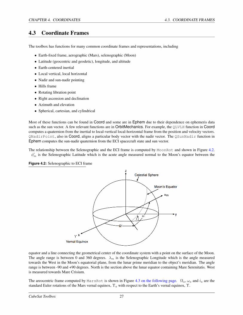
The areocentric frame computed by MarsRot is shown in Figure 4.3 on the following page. Ωa, ωa and ia are thestandard Euler rotations of the Mars vernal equinox, Υa with respect to the Earth’s vernal equinox, Υ.

CubeSat Toolbox 27

4.3. COORDINATE FRAMES CHAPTER 4. COORDINATES

Figure 4.3: Areocentric frame

CubeSat Toolbox 28

CHAPTER 5

PLANETARY AND SUN EPHEMERIS

5.1 Overview

The Ephem directory provides functions for time-dependent information such as finding planet, moon, and sun loca-tions; coordinate frame transformations; time transformations; solstice, equinox, and eclipses. There also utilities fordrawing ground tracks, finding Lagrange points, and computing parallax. Functions for attitude frames related to thesun vector are also found here, such as sun-nadir (QSunNadir) and sun-pointing (QSunPointing). Type helpEphem for a full listing.

There are demos for finding Earth nutation, precession, and rotation (TEarth); eclipses (TEclipse); and the sim-plified planets model (TPlanets).

The most recent additions to the toolbox ephemeris capability include an interface to the JPL ephemerides and func-tions more suited to use in interplanetary orbits, such as SunVectorECI in addition to SunV1 and SunV2.

The CubeSat Toolbox contains only a subset of these functions, including SunV1, MoonV1, Planets, and ECIToEF,which is a computationally fast almanac version of the transformation from ECI to the Earth-fixed frame.

5.2 Almanac functions

The toolbox has a variety of almanac functions for obtaining the ephemeris of the planets1, moon, and sun. Forexample, the following functions are available in Ephem:

• MoonV1 2

• MoonV2 3

• Planets, PlanetPosition 4

• SolarSys

• SunV1 5

• SunV2 6

1Explanatory Supplement to the Astronomical Almanac (1992.) Table 5.8.1. p. 316.2The 1993 Astronomical Almanac, p. D46.3Montenbruck, O., Pfleger, T., Astronomy on the Personal Computer, Springer-Verlag, Berlin, 1991, pp. 103-111.4Explanatory Supplement to the Astronomical Almanac, 1992, p. 316.5 The 1993 Astronomical Almanac, p. C24.6Montenbruck and Pfleger, p. 36.

29

5.3. JPL EPHEMERIS CHAPTER 5. EPHEMERIS

5.3 JPL Ephemeris

The toolbox has the capability to use a JPL ephemeris file such as the DE405 set within the Toolbox. The functionsPlanetPosJPL and SolarSysJPL provide equivalence to PlanetPosition and SolarSys.

NASA’s Jet Propulsion Laboratory (JPL) freely provides these ASCII Lunar and Planetary Ephemerides which can bedownloaded from its website at the ftp site at ftp://ssd.jpl.nasa.gov/pub/eph/export with help athttp://ssd.jpl.nasa.gov/?planet eph export. The functions used in the toolbox for the purpose of reading and interpo-lating these JPL ephemeris files are based on a C implementation by David Hoffman (Johnson Space Center) availableon the ftp site. They generate state data (position and velocity) for the sun, earth’s moon and the 9 major planets.The MATLAB functions require binary versions of the ephemeris which are system-dependent and therefore must becreated by users.

5.3.1 Creating and managing binary files of the JPL ephemerides

Users will first need to compile binary versions of the ASCII files on their own system. This can be done with anyof a number of tools available from the website. The ASCII files are available in 20 year units, i.e. ASCP2000.405,ASCP2020.405. The conversion also needs the header file HEADERPO.405. If you compile Hoffman’s C utility onyour computer, you could for example do

$ ./convert header.405 ascp2000.405 bin2000.405

Writing record: 25Writing record: 50Writing record: 75Writing record: 100Writing record: 125Writing record: 150Writing record: 175Writing record: 200Writing record: 225

Data Conversion Completed.

Records Converted: 230Records Rejected: 0

and similarly create a file for bin2020.405. To verify the files, you can use print header and scan records.

$ ./print_header bin2020.405

GROUP 1010

JPL Planetary Ephemeris DE405/DE405Start Epoch: JED= 2305424.5 1599 DEC 09 00:00:00

Final Epoch: JED= 2525008.5 2201 FEB 2000:00:00

GROUP 1030

2305424.50 2525008.50 32.00

GROUP 1040

156DENUM LENUM TDATEF TDATEB CENTER CLIGHT AU EMRAT GM1 GM2GMB GM4 GM5 GM6 GM7 GM8 GM9 GMS RAD1 RAD2

CubeSat Toolbox 30

CHAPTER 5. EPHEMERIS 5.3. JPL EPHEMERIS

RAD4 JDEPOC X1 Y1 Z1 XD1 YD1 ZD1 X2 Y2Z2 XD2 YD2 ZD2 XB YB ZB XDB YDB ZDBX4 Y4 Z4 XD4 YD4 ZD4 X5 Y5 Z5 XD5YD5 ZD5 X6 Y6 Z6 XD6 YD6 ZD6 X7 Y7Z7 XD7 YD7 ZD7 X8 Y8 Z8 XD8 YD8 ZD8X9 Y9 Z9 XD9 YD9 ZD9 XM YM ZM XDMYDM ZDM XS YS ZS XDS YDS ZDS BETA GAMMAJ2SUN GDOT MA0001 MA0002 MA0004 MAD1 MAD2 MAD3 RE ASUNPHI THT PSI OMEGAX OMEGAY OMEGAZ AM J2M J3M J4MC22M C31M C32M C33M S31M S32M S33M C41M C42M C43MC44M S41M S42M S43M S44M LBET LGAM K2M TAUM AEJ2E J3E J4E K2E0 K2E1 K2E2 TAUE0 TAUE1 TAUE2 DROTEXDROTEY GMAST1 GMAST2 GMAST3 KVC IFAC PHIC THTC PSIC OMGCXOMGCY OMGCZ PSIDOT MGMIS ROTEX ROTEY

$ ./scan_records bin2000.405

Record Start Stop-----------------------------------

1 2451536.50 2451568.502 2451568.50 2451600.50...

230 2458832.50 2458864.50

You can concatenate the files using append. In this case, the data from the second binary file is added to the first.When you scan the records of the combined file the number is increased from 230 to 458. There is also a function toenable you to extract records from binary files to create a custom time interval.

$ mv bin2000.405 binEphem.405$ ./append binEphem.405 bin2020.40$ ./scan_records binEphem.405

Record Start Stop-----------------------------------

1 2451536.50 2451568.502 2451568.50 2451600.50...

458 2466128.50 2466160.50

5.3.2 The InterpolateState function

The function which directly interfaces with the JPL ephemeris files is InterpolateState. This function returnsthe state of a single body at a specific Julian Date. The state is measured from the solar system barycenter and in themean Earth equator frame. The function call is

[X, GM] = InterpolateState( Target, Time, fileName )

The numbering convention for the Target bodies is given in table Table 5.1 on the next page: Additional compu-tations are required to obtain planet states referenced from the sun, or to obtain the heliocentric positions of the Earthand moon.

5.3.3 JPL Ephemeris Demos

The function InterpolateState has its own built-in demo. Recall that this state is measured from the solarsystem barycenter and is in the Earth equatorial frame.

State for Mercury on Jan 1, 20012.454786013744712e+07-5.399651407895338e+07

CubeSat Toolbox 31

5.3. JPL EPHEMERIS CHAPTER 5. EPHEMERIS

Table 5.1: Target Numbering Convention

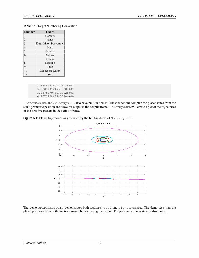
Number Bodies1 Mercury2 Venus3 Earth-Moon Barycenter4 Mars5 Jupiter6 Saturn7 Uranus8 Neptune9 Pluto10 Geocentric Moon11 Sun

-3.136647347180613e+073.530110141765838e+011.987507976959802e+016.957125863787630e+00

PlanetPosJPL and SolarSysJPL also have built-in demos. These functions compute the planet states from thesun’s geometric position and allow for output in the ecliptic frame. SolarSysJPLwill create a plot of the trajectoriesof the first five planets in the ecliptic frame.

Figure 5.1: Planet trajectories as generated by the built-in demo of SolarSysJPL

−6 −4 −2 0 2 4 6−6

−4

−2

0

2

4

6

x

y

Trajectories in AU

−5 −4 −3 −2 −1 0 1 2 3 4

−1.5

−1

−0.5

0

0.5

1

1.5

x

z

The demo JPLPlanetDemo demonstrates both SolarSysJPL and PlanetPosJPL. The demo tests that theplanet positions from both functions match by overlaying the output. The geocentric moon state is also plotted.

CubeSat Toolbox 32

CHAPTER 6

CUBESAT

This chapter discusses how to use the CubeSat module. This module provides special system modules and missionplanning tools suitable for nanosatellite design.

The organization of the module can be seen by typing

>> help CubeSat

which returns a list of folders in the module. This includes Simulation, MissionPlanning, and Visualization, alongwith corresponding Demos folders.

The CubeSat integrated simulation includes a simplified surface model for calculating disturbances. The toolboxincludes the following features:

• Integrated simulation model including

– Rigid body dynamics

– Reaction wheel gyrostat dynamics

– Point mass

– Scale height and Jacchia atmospheric models

– Magnetic dipole, drag, and optical force models

– Gravity gradient torques

– Solar cell power model including battery charging dynamics

• Three-axis attitude control using a PID

• Momentum unloading calculations

• Model attitude damping such as with magnetic hysteresis rods

• 2D and 3D visualization including

– Model visualization with surface normals

– 2D and 3D orbit plotting

– 3D attitude visualization

• Ephemeris

– Convert ECI to Earth-fixed using almanac models

– Sun vector

33

6.1. CUBESAT MODELING CHAPTER 6. CUBESAT

– Moon vector

• Advanced orbit dynamics

– Spherical harmonic gravity model

– Relative orbit dynamics between two close satellites

• Observation time windows

• Subsystem models

– Link bit error probabilities

– Isothermal spacecraft model

– Cold gas propulsion

6.1 CubeSat Modeling

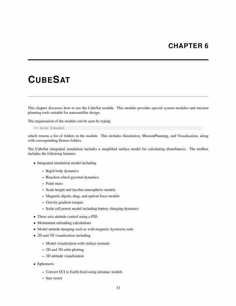
The CubeSat model is generated by CubeSatModel, in the Utilities folder. The default demo creates a 2U satellite.The model is essentially a set of vertices and faces defining the exterior of the satellite. The function header is belowand the resulting model is in Figure 6.1 on the facing page. This model has 152 faces.

>> help CubeSatModelGenerate vertices and faces for a CubeSat model.If there are no outputs it will generate a plot with surface normals, oryou can draw the cubesat model using patch:

patch(’vertices’,v,’faces’,f,’facecolor’,[0.5 0.5 0.5]);

type can be ’3U’ or [3 2 1] i.e. a different dimension for x, y and z.

Type CubeSatModel for a demo of a 3U CubeSat.

This function will populate dRHS for use in RHSCubeSat. The surfacedata for the cube faces will be 6 surfaces that are the dimensions ofthe core spacecraft. Additional surfaces are added for the deployablesolar panels. Solar panels are grouped into wings that attached to theedges of the CubeSat.

The function computes the inertia matrix, center of mass and totalmass. The mass properties of the interior components are computed fromtotal mass and center of mass.

If you set frameOnly to true (or 1), v and f will not contain thewalls. However, dRHS will contain all the wall properties.--------------------------------------------------------------------------

Form:d = CubeSatModel( ’struct’ )[v, f] = CubeSatModel( type, t )[v, f, dRHS] = CubeSatModel( type, d, frameOnly )Demo:CubeSatModel

--------------------------------------------------------------------------

------Inputs------type (1,:) ’nU’ where n may be any number, or [x y z]d (.) Data structure for the CubeSat

.thicknessWall (1,1) Wall thickness (mm)

.thicknessRail (1,1) Rail thickness (mm)

.densityWall (1,1) Density of the wall material (kg/m3)

.massComponents (1,1) Interior component mass (kg)

CubeSat Toolbox 34

CHAPTER 6. CUBESAT 6.1. CUBESAT MODELING

.cMComponents (1,1) Interior components center of mass

.sigma (3,6) [absorbed; specular; diffuse]

.cD (1,6) Drag coefficient

.solarPanel.dim (3,1) [side attached to cubesat, side perpendicular,thickness]

.solarPanel.nPanels (1,1) Number of panels per wing

.solarPanel.rPanel (3,w) Location of inner edge of panel

.solarPanel.sPanel (3,w) Direction of wing spine

.solarPanel.cellNormal (3,w) Wing cell normal

.solarPanel.sigmaCell (3,1) [absorbed; specular; diffuse] coefficients

.solarPanel.sigmaBack (3,1) [absorbed; specular; diffuse]

.solarPanel.mass (1,1) Panel mass- OR -

t (1,1) Wall thickness (mm)frameOnly (1,1) If true just draw the frame, optional

-------Outputs-------v (:,3) Verticesf (:,3) FacesdRHS (1,1) Data structure for the function RHSCubeSat

--------------------------------------------------------------------------Reference: CubeSat Design Specification (CDS) Revision 9

--------------------------------------------------------------------------

Figure 6.1: Model of 2U CubeSat

For the purposes of disturbance analysis, the CubeSat module uses a simplified model of areas and normals. SeeCubeSatFaces. The CubeSatModel function will output a data structure with the surface model in addition tothe vertices and faces, which are strictly for visualization. This function does have the capability to model deployablesolar wings. The solar areas and normals for power generation are specified separately from the satellite surfaces, asthey may be only a portion of any given surface. See SolarCellPower for the power model.

The CubeSatRHS function documents the simulation data model. The function returns a data structure by default forinitializing simulations. The surface data from the CubeSatModel function is in the surfData and power fields.The default data assumes no reaction wheels, as can be seen below since the kWheels field is empty. The atm data

CubeSat Toolbox 35

6.2. SIMULATION CHAPTER 6. CUBESAT

structure contains the atmosphere model data for use with AtmJ70. If this structure is empty, the simpler and fasterscale height model in AtmDens2 will be used instead.

>> d = RHSCubeSatd =

struct with fields:

jD0: 2.4552e+06mass: 1

inertia: 0.0016667dipole: [3?1 double]power: [1?1 struct]

surfData: [1?1 struct]aeroModel: @CubeSatAero

opticalModel: @CubeSatRadiationPressureatm: [1x1 struct]

kWheels: []inertiaRWA: []

tRWA: []

Note in the above structure that the aerodynamics and optical force models are function handles. These functions aredesigned to accept the surface model data structure within RHSCubeSat.

The key functions for modeling CubeSats are summarized in Table 6.1.

Table 6.1: CubeSat Modeling Functions

AddMass Combine component masses and calculate inertia and center-of-mass.InertiaCubeSat Compute the inertia for standard CubeSat types.CubeSatFaces Compute surface areas and normals for the faces of a CubeSat.CubeSatModel Generate vertices and faces for a CubeSat model.TubeSatModel Generate a TubeSat model.

6.2 Simulation

Example simulations are in the Demos/RelativeOrbit and Demos/Simulation folders. The first has a formationflying demo, FFSimDemo. The second has a variety of simulations including an attitude control simulation demo,CubeSatSimulation. CubeSatRWASimulation demonstrates a set of three orthgononal reaction wheels.CubeSatGGStabilized shows how to set up the mass properties for a gravity-gradient boom.

Attitude control loops can be designed using the PIDMIMO function and implemented using PID3Axis. These areincluded from the standard Spacecraft Control Toolbox.

The orbit simulations, TwoSpacecraftSimpleOrbitSimulation and TwoSpacecraftOrbitSimulation, sim-ulate the same orbits, but the simple version uses just the central force model and the second adds a variety of distur-bances. Both use MATLAB’s ode113 function for integration, so that integration occurs on a single line, without afor loop. ode113 is a variable step propagator that may take very long steps for orbit sims. The integration linelooks like

% Numerically integrate the orbit%--------------------------------[t,x] = ode113( @FOrbitMultiSpacecraft, [0 tEnd], x, opt, d );

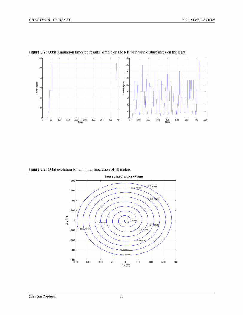
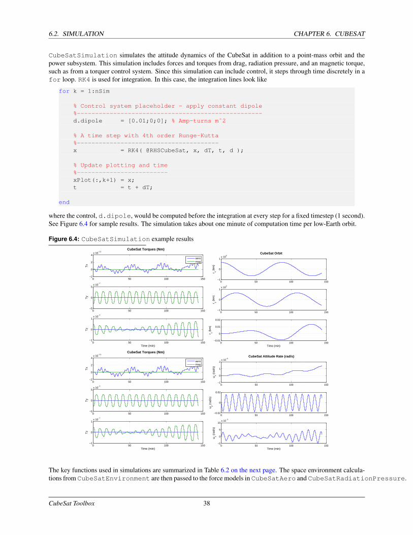
The default simulation length is 12 hours, and the simple sim results in 438 timesteps while the one with disturbancescomputes 733 steps; Figure 6.2 on the facing page compares the time output of the two examples, where we can seethat the simple simulation had mostly a constant step size. Figure 6.3 on the next page shows the typical orbit results.

CubeSat Toolbox 36

CHAPTER 6. CUBESAT 6.2. SIMULATION

Figure 6.2: Orbit simulation timestep results, simple on the left with with disturbances on the right.

0 50 100 150 200 250 300 350 400 4500

20

40

60

80

100

120

Tim

este

p (

sec)

Steps0 100 200 300 400 500 600 700 800

0

20

40

60

80

100

120

140

160

180

Tim

este

p (

sec)

Steps

Figure 6.3: Orbit evolution for an initial separation of 10 meters

Two spacecraft XY−Plane

−800 −600 −400 −200 0 200 400 600 800−800

−600

−400

−200

0

200

400

600

800

∆ y

(m)

∆ x (m)

− 0.0 hours

− 3.8 hours

− 5.4 hours

− 6.6 hours

− 7.6 hours

− 8.5 hours

− 9.4 hours

− 10.1 hours

− 10.8 hours

− 11.5 hours

− 12.0 hours

CubeSat Toolbox 37

6.2. SIMULATION CHAPTER 6. CUBESAT

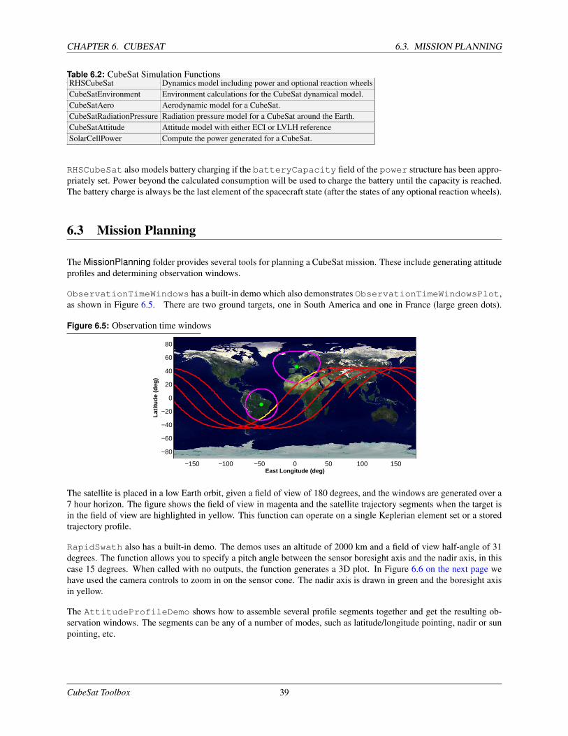
CubeSatSimulation simulates the attitude dynamics of the CubeSat in addition to a point-mass orbit and thepower subsystem. This simulation includes forces and torques from drag, radiation pressure, and an magnetic torque,such as from a torquer control system. Since this simulation can include control, it steps through time discretely in afor loop. RK4 is used for integration. In this case, the integration lines look like

for k = 1:nSim

% Control system placeholder - apply constant dipole%---------------------------------------------------d.dipole = [0.01;0;0]; % Amp-turns mˆ2

% A time step with 4th order Runge-Kutta%---------------------------------------x = RK4( @RHSCubeSat, x, dT, t, d );

% Update plotting and time%-------------------------xPlot(:,k+1) = x;t = t + dT;

end

where the control, d.dipole, would be computed before the integration at every step for a fixed timestep (1 second).See Figure 6.4 for sample results. The simulation takes about one minute of computation time per low-Earth orbit.

Figure 6.4: CubeSatSimulation example resultsCubeSat Torques (Nm)

0 50 100 150−2

0

2

4x 10

−11

Tx

0 50 100 150−5

0

5x 10

−7

Ty

0 50 100 150−1

0

1x 10

−7

Tz

Time (min)

aeromag

CubeSat Orbit

0 50 100 150−1

0

1x 10

4

r x (km

)

0 50 100 150−1

0

1x 10

4

r y (km

)

0 50 100 150−0.01

0

0.01

0.02

r z (km

)

Time (min)

CubeSat Torques (Nm)

0 50 100 150−2

0

2

4x 10

−11

Tx

0 50 100 150−5

0

5x 10

−7

Ty

0 50 100 150−1

0

1x 10

−7

Tz

Time (min)

aeromag

CubeSat Attitude Rate (rad/s)

0 50 100 150−1

0

1

2x 10

−5

ωx (

rad/

s)

0 50 100 150−0.02

0

0.02

ωy (

rad/

s)

0 50 100 150−5

0

5

10x 10

−3

ωz (

rad/

s)

Time (min)

The key functions used in simulations are summarized in Table 6.2 on the next page. The space environment calcula-tions from CubeSatEnvironment are then passed to the force models in CubeSatAero and CubeSatRadiationPressure.

CubeSat Toolbox 38

CHAPTER 6. CUBESAT 6.3. MISSION PLANNING

Table 6.2: CubeSat Simulation FunctionsRHSCubeSat Dynamics model including power and optional reaction wheelsCubeSatEnvironment Environment calculations for the CubeSat dynamical model.CubeSatAero Aerodynamic model for a CubeSat.CubeSatRadiationPressure Radiation pressure model for a CubeSat around the Earth.CubeSatAttitude Attitude model with either ECI or LVLH referenceSolarCellPower Compute the power generated for a CubeSat.

RHSCubeSat also models battery charging if the batteryCapacity field of the power structure has been appro-priately set. Power beyond the calculated consumption will be used to charge the battery until the capacity is reached.The battery charge is always be the last element of the spacecraft state (after the states of any optional reaction wheels).

6.3 Mission Planning

The MissionPlanning folder provides several tools for planning a CubeSat mission. These include generating attitudeprofiles and determining observation windows.

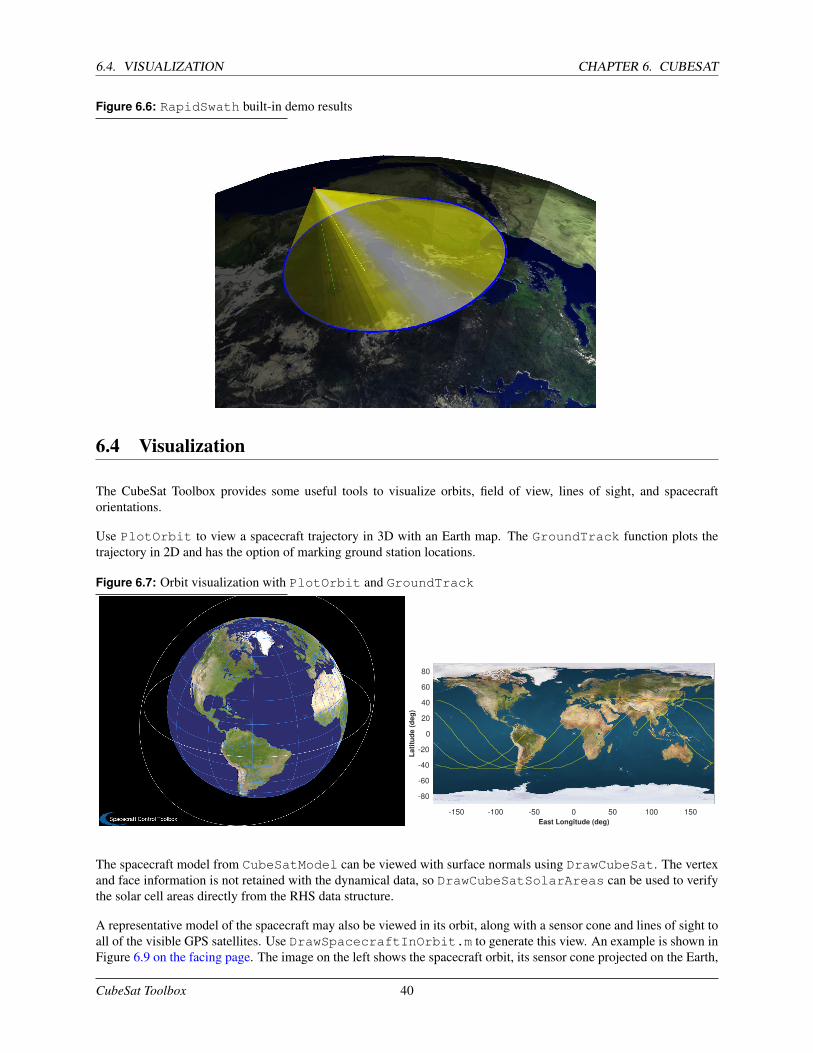
ObservationTimeWindows has a built-in demo which also demonstrates ObservationTimeWindowsPlot,as shown in Figure 6.5. There are two ground targets, one in South America and one in France (large green dots).

Figure 6.5: Observation time windows

−150 −100 −50 0 50 100 150

−80

−60

−40

−20

0

20

40

60

80

East Longitude (deg)

Lat

itu

de

(deg

)

The satellite is placed in a low Earth orbit, given a field of view of 180 degrees, and the windows are generated over a7 hour horizon. The figure shows the field of view in magenta and the satellite trajectory segments when the target isin the field of view are highlighted in yellow. This function can operate on a single Keplerian element set or a storedtrajectory profile.

RapidSwath also has a built-in demo. The demos uses an altitude of 2000 km and a field of view half-angle of 31degrees. The function allows you to specify a pitch angle between the sensor boresight axis and the nadir axis, in thiscase 15 degrees. When called with no outputs, the function generates a 3D plot. In Figure 6.6 on the next page wehave used the camera controls to zoom in on the sensor cone. The nadir axis is drawn in green and the boresight axisin yellow.

The AttitudeProfileDemo shows how to assemble several profile segments together and get the resulting ob-servation windows. The segments can be any of a number of modes, such as latitude/longitude pointing, nadir or sunpointing, etc.

CubeSat Toolbox 39

6.4. VISUALIZATION CHAPTER 6. CUBESAT

Figure 6.6: RapidSwath built-in demo results

6.4 Visualization

The CubeSat Toolbox provides some useful tools to visualize orbits, field of view, lines of sight, and spacecraftorientations.

Use PlotOrbit to view a spacecraft trajectory in 3D with an Earth map. The GroundTrack function plots thetrajectory in 2D and has the option of marking ground station locations.

Figure 6.7: Orbit visualization with PlotOrbit and GroundTrack

-150 -100 -50 0 50 100 150

East Longitude (deg)

-80

-60

-40

-20

0

20

40

60

80

La

titu

de

(d

eg

)

The spacecraft model from CubeSatModel can be viewed with surface normals using DrawCubeSat. The vertexand face information is not retained with the dynamical data, so DrawCubeSatSolarAreas can be used to verifythe solar cell areas directly from the RHS data structure.

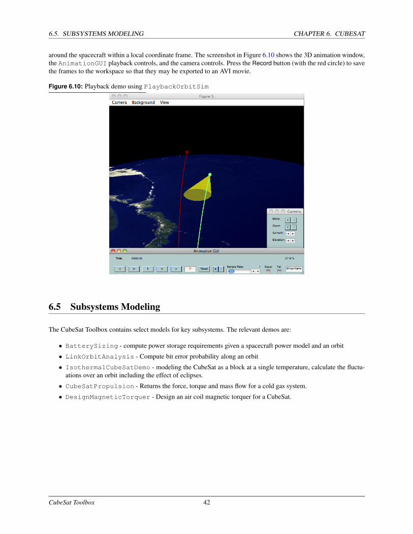
A representative model of the spacecraft may also be viewed in its orbit, along with a sensor cone and lines of sight toall of the visible GPS satellites. Use DrawSpacecraftInOrbit.m to generate this view. An example is shown inFigure 6.9 on the facing page. The image on the left shows the spacecraft orbit, its sensor cone projected on the Earth,

CubeSat Toolbox 40

CHAPTER 6. CUBESAT 6.4. VISUALIZATION

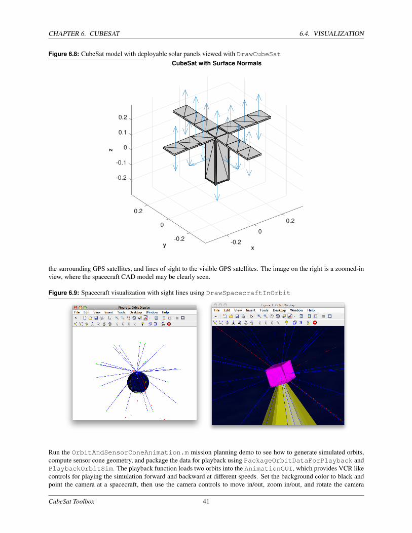
Figure 6.8: CubeSat model with deployable solar panels viewed with DrawCubeSat

-0.2

-0.1

0.2

0z

0.1

CubeSat with Surface Normals

0.2

0.2

y

0

x

0

-0.2-0.2

the surrounding GPS satellites, and lines of sight to the visible GPS satellites. The image on the right is a zoomed-inview, where the spacecraft CAD model may be clearly seen.

Figure 6.9: Spacecraft visualization with sight lines using DrawSpacecraftInOrbit

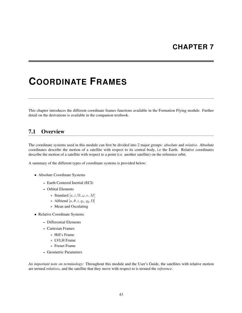
Run the OrbitAndSensorConeAnimation.m mission planning demo to see how to generate simulated orbits,compute sensor cone geometry, and package the data for playback using PackageOrbitDataForPlayback andPlaybackOrbitSim. The playback function loads two orbits into the AnimationGUI, which provides VCR likecontrols for playing the simulation forward and backward at different speeds. Set the background color to black andpoint the camera at a spacecraft, then use the camera controls to move in/out, zoom in/out, and rotate the camera

CubeSat Toolbox 41

6.5. SUBSYSTEMS MODELING CHAPTER 6. CUBESAT

around the spacecraft within a local coordinate frame. The screenshot in Figure 6.10 shows the 3D animation window,the AnimationGUI playback controls, and the camera controls. Press the Record button (with the red circle) to savethe frames to the workspace so that they may be exported to an AVI movie.

Figure 6.10: Playback demo using PlaybackOrbitSim

6.5 Subsystems Modeling

The CubeSat Toolbox contains select models for key subsystems. The relevant demos are:

• BatterySizing - compute power storage requirements given a spacecraft power model and an orbit

• LinkOrbitAnalysis - Compute bit error probability along an orbit

• IsothermalCubeSatDemo - modeling the CubeSat as a block at a single temperature, calculate the fluctu-ations over an orbit including the effect of eclipses.

• CubeSatPropulsion - Returns the force, torque and mass flow for a cold gas system.

• DesignMagneticTorquer - Design an air coil magnetic torquer for a CubeSat.

CubeSat Toolbox 42

CHAPTER 7

COORDINATE FRAMES

This chapter introduces the different coordinate frames functions available in the Formation Flying module. Furtherdetail on the derivations is available in the companion textbook.

7.1 Overview

The coordinate systems used in this module can first be divided into 2 major groups: absolute and relative. Absolutecoordinates describe the motion of a satellite with respect to its central body, i.e the Earth. Relative coordinatesdescribe the motion of a satellite with respect to a point (i.e. another satellite) on the reference orbit.

A summary of the different types of coordinate systems is provided below:

• Absolute Coordinate Systems

– Earth Centered Inertial (ECI)

– Orbital Elements

∗ Standard [a, i,Ω, ω, e,M ]

∗ Alfriend [a, θ, i, q1, q2,Ω]

∗ Mean and Osculating

• Relative Coordinate Systems

– Differential Elements

– Cartesian Frames

∗ Hill’s Frame∗ LVLH Frame∗ Frenet Frame

– Geometric Parameters

An important note on terminology: Throughout this module and the User’s Guide, the satellites with relative motionare termed relatives, and the satellite that they move with respect to is termed the reference.

43

7.2. ORBITAL ELEMENT SETS CHAPTER 7. COORDINATE FRAMES

7.2 Orbital Element Sets

The Formation Flying module makes use of two different orbital element sets. The classical Kepler elements aredefined as:

[a, i,Ω, ω, e,M ]

where a is the semi-major axis, i is the inclination, Ω is the right ascension (longitude) of the ascending node, ω isthe argument of perigee, e is the eccentricity, and M is the mean anomaly. This is the standard set of elements usedthroughout the Spacecraft Control Toolbox.

A second set of elements is particularly useful for formation flying applications. This set is termed the Alfriendelement set, after Dr. Terry Alfriend of Texas A&M who first suggested its use. The Alfriend elements are used solelywith circular or near-circular orbits. The Alfriend set is:

[a, θ, i, q1, q2,Ω]

where a, i,Ω are defined as before. The remaining elements, q1, q2, θ, are defined in order to avoid the problem thatarises at zero eccentricity, where the classical argument of perigee and mean anomaly are undefined.

The functions Alfriend2El and El2Alfriend can be used to convert between the two element sets.

Either of the two above element sets can be defined as mean or osculating. When orbits are governed by a point-massmodel for the central body’s gravity field, the elements do not osculate. Higher fidelity models have perturbations thatcause the elements to change over time, or osculate. The function Osc2Mean will convert osculating elements tomean elements. The elements must be defined in the Alfriend system. Similarly, the function ECI2MeanElementswill compute the mean elements directly from an ECI state.

7.3 Relative Coordinate Systems

The three different types of coordinate systems for expressing the relative orbital states of spacecraft are described inthe textbook: orbital element differences, cartesian coordinate systems, and geometric parameter sets . The FormationFlying module provides coordinate transformation utilities to switch back and forth between all three systems.

7.3.1 Orbital Element Differences

A differential orbital element vector is simply the difference between the orbital element vectors of two satellites. Justas with regular, absolute orbits, this is a convenient way to parameterize the motion of a relative orbit. In the absenceof disturbances and gravitational perturbations, 5 of the 6 differential orbital elements remain fixed; only the mean (ortrue) anomaly changes.

The function OrbElemDiff can be used to robustly subtract two element vectors. This function ensures that angledifferences around the wrapping points of ±π and (0, 2π) are computed properly.

7.3.2 Cartesian Coordinate Systems

The three different coordinate systems for relative orbital motion supported by the Formation Flying module are:

• Hills

• LVLH

CubeSat Toolbox 44

CHAPTER 7. COORDINATE FRAMES 7.3. RELATIVE COORDINATE SYSTEMS

• Frenet

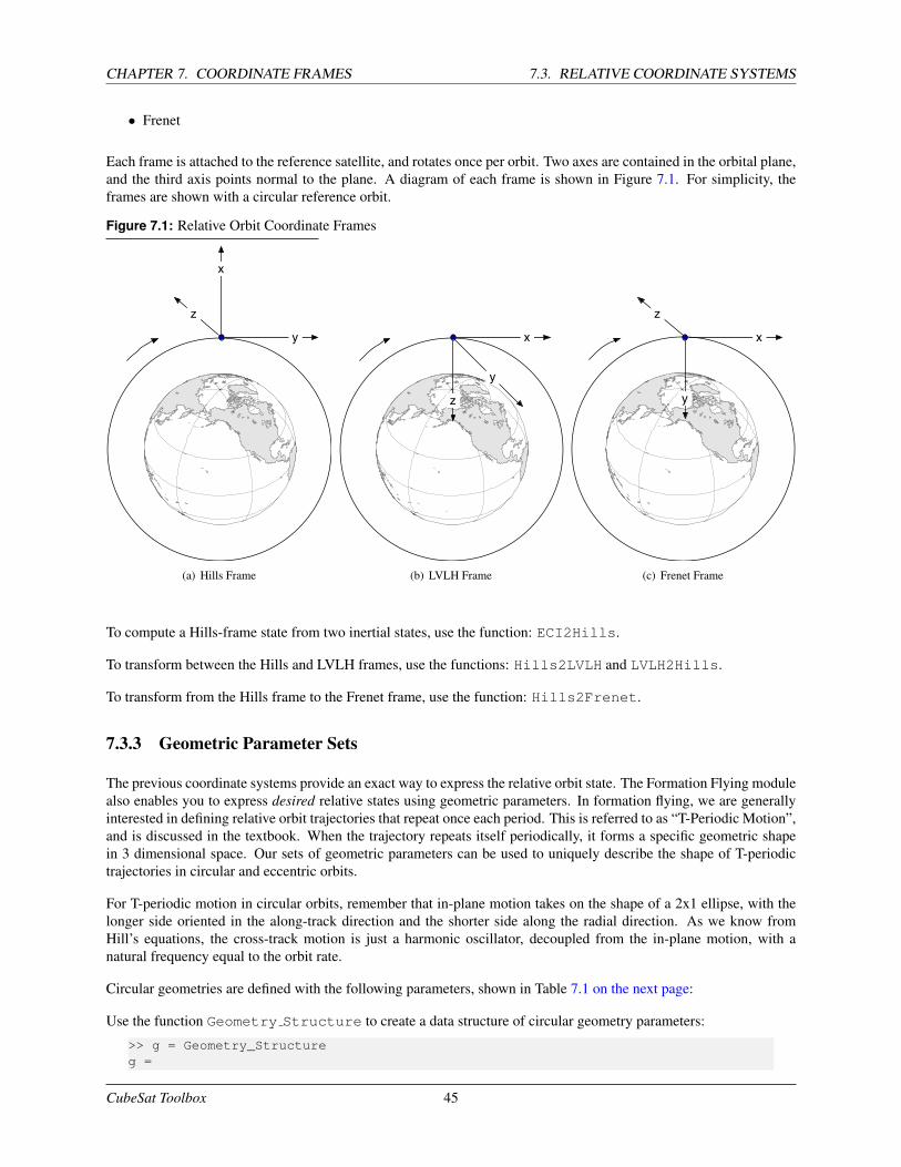
Each frame is attached to the reference satellite, and rotates once per orbit. Two axes are contained in the orbital plane,and the third axis points normal to the plane. A diagram of each frame is shown in Figure 7.1. For simplicity, theframes are shown with a circular reference orbit.

Figure 7.1: Relative Orbit Coordinate Frames

x

y

z

(a) Hills Frame

z

x

y

(b) LVLH Frame

y

x

z

(c) Frenet Frame

To compute a Hills-frame state from two inertial states, use the function: ECI2Hills.

To transform between the Hills and LVLH frames, use the functions: Hills2LVLH and LVLH2Hills.

To transform from the Hills frame to the Frenet frame, use the function: Hills2Frenet.

7.3.3 Geometric Parameter Sets

The previous coordinate systems provide an exact way to express the relative orbit state. The Formation Flying modulealso enables you to express desired relative states using geometric parameters. In formation flying, we are generallyinterested in defining relative orbit trajectories that repeat once each period. This is referred to as “T-Periodic Motion”,and is discussed in the textbook. When the trajectory repeats itself periodically, it forms a specific geometric shapein 3 dimensional space. Our sets of geometric parameters can be used to uniquely describe the shape of T-periodictrajectories in circular and eccentric orbits.

For T-periodic motion in circular orbits, remember that in-plane motion takes on the shape of a 2x1 ellipse, with thelonger side oriented in the along-track direction and the shorter side along the radial direction. As we know fromHill’s equations, the cross-track motion is just a harmonic oscillator, decoupled from the in-plane motion, with anatural frequency equal to the orbit rate.

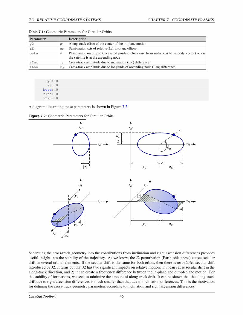
Circular geometries are defined with the following parameters, shown in Table 7.1 on the next page:

Use the function Geometry Structure to create a data structure of circular geometry parameters:

>> g = Geometry_Structureg =

CubeSat Toolbox 45

7.3. RELATIVE COORDINATE SYSTEMS CHAPTER 7. COORDINATE FRAMES

Table 7.1: Geometric Parameters for Circular Orbits

Parameter Descriptiony0 y0 Along-track offset of the center of the in-plane motionaE aE Semi-major axis of relative 2x1 in-plane ellipsebeta β Phase angle on ellipse (measured positive clockwise from nadir axis to velocity vector) when

the satellite is at the ascending nodezInc zi Cross-track amplitude due to inclination (Inc) differencezLan zΩ Cross-track amplitude due to longitude of ascending node (Lan) difference

y0: 0aE: 0

beta: 0zInc: 0zLan: 0

A diagram illustrating these parameters is shown in Figure 7.2.

Figure 7.2: Geometric Parameters for Circular Orbits

yH

|z|

aE2

β0

xH xH

yHzH

aE|z| y0

xH

yH

zH

aEy0

|z|

xH

zH

|z||z|

aE

y0

Separating the cross-track geometry into the contributions from inclination and right ascension differences providesuseful insight into the stability of the trajectory. As we know, the J2 perturbation (Earth oblateness) causes seculardrift in several orbital elements. If the secular drift is the same for both orbits, then there is no relative secular driftintroduced by J2. It turns out that J2 has two significant impacts on relative motion: 1) it can cause secular drift in thealong-track direction, and 2) it can create a frequency difference between the in-plane and out-of-plane motion. Forthe stability of formations, we seek to minimize the amount of along-track drift. It can be shown that the along-trackdrift due to right ascension differences is much smaller than that due to inclination differences. This is the motivationfor defining the cross-track geometry parameters according to inclination and right ascension differences.

CubeSat Toolbox 46

CHAPTER 7. COORDINATE FRAMES 7.3. RELATIVE COORDINATE SYSTEMS

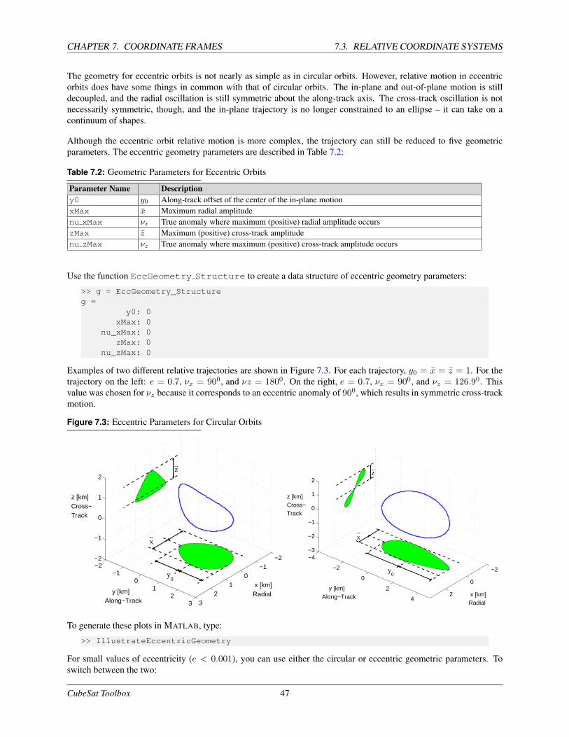
The geometry for eccentric orbits is not nearly as simple as in circular orbits. However, relative motion in eccentricorbits does have some things in common with that of circular orbits. The in-plane and out-of-plane motion is stilldecoupled, and the radial oscillation is still symmetric about the along-track axis. The cross-track oscillation is notnecessarily symmetric, though, and the in-plane trajectory is no longer constrained to an ellipse – it can take on acontinuum of shapes.

Although the eccentric orbit relative motion is more complex, the trajectory can still be reduced to five geometricparameters. The eccentric geometry parameters are described in Table 7.2:

Table 7.2: Geometric Parameters for Eccentric Orbits

Parameter Name Descriptiony0 y0 Along-track offset of the center of the in-plane motionxMax x Maximum radial amplitudenu xMax νx True anomaly where maximum (positive) radial amplitude occurszMax z Maximum (positive) cross-track amplitudenu zMax νz True anomaly where maximum (positive) cross-track amplitude occurs

Use the function EccGeometry Structure to create a data structure of eccentric geometry parameters:

>> g = EccGeometry_Structureg =

y0: 0xMax: 0

nu_xMax: 0zMax: 0

nu_zMax: 0

Examples of two different relative trajectories are shown in Figure 7.3. For each trajectory, y0 = x = z = 1. For thetrajectory on the left: e = 0.7, νx = 900, and νz = 1800. On the right, e = 0.7, νx = 900, and νz = 126.90. Thisvalue was chosen for νz because it corresponds to an eccentric anomaly of 900, which results in symmetric cross-trackmotion.

Figure 7.3: Eccentric Parameters for Circular Orbits

−2−1

01

23

−2−1

01

23

−2

−1

0

1

2

x [km]Radial

z_

y0

x_

y [km]Along−Track

z [km]Cross−Track

−2

0

2

−4

−2

0

2

4

−3

−2

−1

0

1

2

x [km]Radial

y0

z_

x_

y [km]Along−Track

z [km]Cross−Track

To generate these plots in MATLAB, type:

>> IllustrateEccentricGeometry

For small values of eccentricity (e < 0.001), you can use either the circular or eccentric geometric parameters. Toswitch between the two:

CubeSat Toolbox 47

7.3. RELATIVE COORDINATE SYSTEMS CHAPTER 7. COORDINATE FRAMES

gEcc = GeometryCirc2Ecc( w, gCirc );gCirc = GeometryEcc2Circ( w, gEcc );

where w is the argument of perigee.

A number of transformation functions are provided in the Transformation folder. The following table summarizesthe different transformations between various coordinate frames that are possible. The notation x refers to a state withposition and velocity, e is an orbital element set, and g is a set of geometric parameters. The ∆ prefix indicates arelative state. The subscripts are defined as: H (Hills), L (LVLH), F (Frenet), S (Standard), A (Alfriend), C (Circular),E (Eccentric).

Table 7.3: Coordinate Transformations

xECI eS eA ∆xH ∆xL ∆xF ∆eS ∆eA ∆gC ∆gExECI -

√ √ √

eS√

-√ √

eA√

-√

∆xH√

-√ √ √ √ √ √

∆xL√ √

-∆xF

√-

∆eS√ √

-√ √ √

∆eA√ √ √

-√ √

∆gC√ √ √

-√

∆gE√ √ √ √

-

CubeSat Toolbox 48

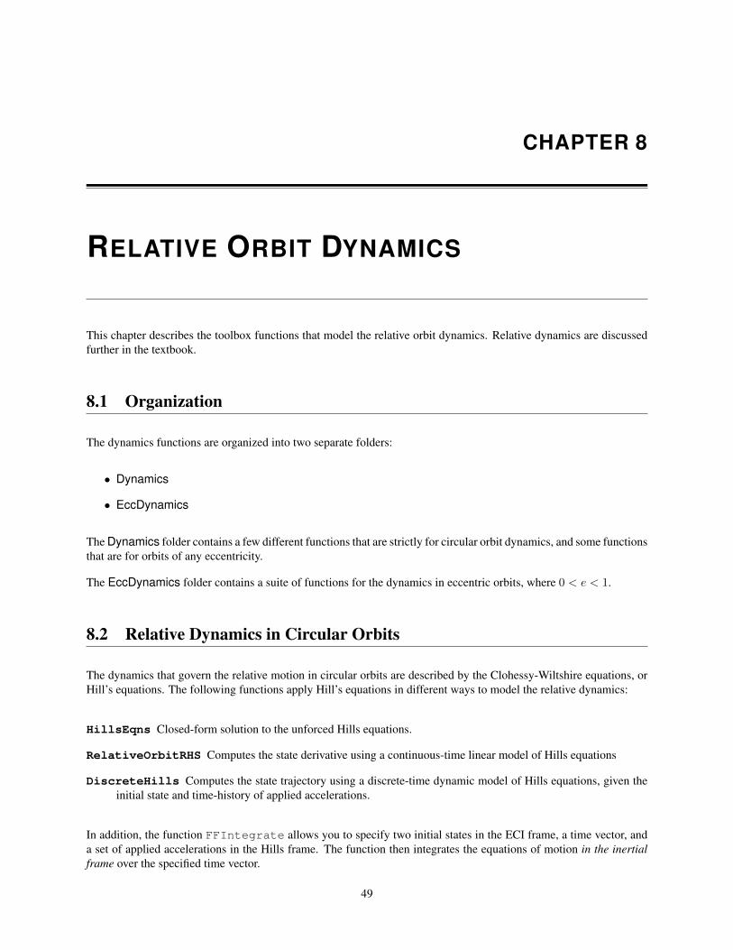
CHAPTER 8

RELATIVE ORBIT DYNAMICS

This chapter describes the toolbox functions that model the relative orbit dynamics. Relative dynamics are discussedfurther in the textbook.

8.1 Organization

The dynamics functions are organized into two separate folders:

• Dynamics

• EccDynamics

The Dynamics folder contains a few different functions that are strictly for circular orbit dynamics, and some functionsthat are for orbits of any eccentricity.

The EccDynamics folder contains a suite of functions for the dynamics in eccentric orbits, where 0 < e < 1.

8.2 Relative Dynamics in Circular Orbits

The dynamics that govern the relative motion in circular orbits are described by the Clohessy-Wiltshire equations, orHill’s equations. The following functions apply Hill’s equations in different ways to model the relative dynamics:

HillsEqns Closed-form solution to the unforced Hills equations.

RelativeOrbitRHS Computes the state derivative using a continuous-time linear model of Hills equations

DiscreteHills Computes the state trajectory using a discrete-time dynamic model of Hills equations, given theinitial state and time-history of applied accelerations.

In addition, the function FFIntegrate allows you to specify two initial states in the ECI frame, a time vector, anda set of applied accelerations in the Hills frame. The function then integrates the equations of motion in the inertialframe over the specified time vector.

49

8.3. RELATIVE DYNAMICS IN ECCENTRIC ORBITS CHAPTER 8. RELATIVE ORBIT DYNAMICS

The function HillsEqns gives a closed-form solution for the relative position and velocity at a future time, giventhe initial position and velocity, and the orbit rate.

Example 8.1 shows a short script that simulates 1 orbit, along with a plot of the trajectory.

Example 8.1 Example Trajectory Found with HillsEqns.m

1 % orbit rate (rad/s)2 n = .001;3

4 % time vector5 t = linspace(0,2*pi/n,100);6

7 % initial state8 xH0 = [1;0;1;0;-2*n;0];9

10 % state trajectory over time t11 xH = HillsEqns( xH0, n, t, 1 );12

13 % plot14 HillsFramePlot(xH)

−2

−1

0

1

2

7 8 9 10 11 12 13

−2

0

2

y [km]Along−Track

z [km]Cross−Track

x [km]Radial

We first define the orbit rate and a time vector that spans one orbit. We then define the initial state, xH0. The initial xposition is 1 km, and the initial y velocity is −.002 km/s. This results in T-periodic motion. The fourth input providedto HillsEqns.m is a flag, where 1 gives the output as a 6 × 1 vector, and the 2 gives the output as a data structurewith fields for position, velocity and time.

The function RelativeOrbitRHS can be used as the right-hand-side equation in a numerical integration routine.

Example 8.2 on the facing page shows a short script that simulates 3 orbits, along with a plot of the trajectory. Noticethe initial y velocity is changed slightly from the previous amount, resulting in along-track drift. Also, notice that theapplied acceleration is an input. Here, we simply set it to zero. However, this can be used to model both disturbanceand control accelerations.

The function DiscreteHills provides a discrete-time model of the relative dynamics. Given an initial state and atime-history of applied accelerations (spaced at a constant time interval), this function will return the forced relativetrajectory.

8.3 Relative Dynamics in Eccentric Orbits

The equations for relative motion in eccentric orbits can be expressed in a number of different ways. The FormationFlying module implements Lawden’s equations, which use the true anomaly as the independent variable. Theseequations are valid for an eccentricity range of 0 < e < 1. In particular, we follow the formula presented by Inalhanet.al. (AIAA JGCD v.25 no.1, 2002) for the numerical implementation of the state transition matrix.

Another formulation, presented by Yamanaka and Ankersen in the same journal, uses an alternative approach thatavoids the singularity at e = 0. This formulation may be added in a future version of this module.

A summary of the main functions for relative dynamic modeling in eccentric orbits is provided below. Note thatfunctions beginning with the FFEcc prefix are valid only for eccentric orbits (0 < e < 1).

CubeSat Toolbox 50

CHAPTER 8. RELATIVE ORBIT DYNAMICS 8.3. RELATIVE DYNAMICS IN ECCENTRIC ORBITS

Example 8.2 Example Simulation Using RelativeOrbitRHS

1 % initial state2 n = .001;3 xH0 = [1;0;1;0;-2.1*n;n/2];4

5 % applied acceleration6 u = [0;0;0];7

8 % simulation9 T = 2*pi/n;

10 nOrb = 2;11 t = 0;12 k = 0;13 dT = 2;14 xHs = xH0;15 while( t< nOrb*T ),16 k=k+1;17 t=t+dT;18 xHs(:,k+1) = ...19 RK4( ’RelativeOrbitRHS’, ...20 xHs(:,k), dT, t, n, u );21 end22

23 % plot24 HillsFramePlot( xHs )

−3

−2

−1

0

1

2

−20

24

68

−20

2

y [km]Along−Track

z [km]Cross−Track

x [km]Radial

FFEccIntConst Computes a set of integration constants given the initial Hills frame state, eccentricity, and trueanomaly.

FFEccProp Computes Hills frame state at future true anomalies given integration constants and eccentricity.

FFEccLawdensEqns Computes a set of future Hills frame states given the initial Hills frame state, eccentricity,and true anomaly.

FFEccLinOrb Computes the state space matrices for linearized motion about a given Hills frame state at a giventrue anomaly.

FFEccDiscreteHills Similar to the circular orbit version, DiscreteHills. Uses FFEccLinOrb to com-pute continuous time system, then discretizes with a zero-order hold.

GVEDynamics Computes the state space matrices for linearized motion about a given differential element vector,using Gauss’s variational equations.

DisreteGVE Similar to FFEccDiscreteHills, but based the motion is defined in terms of orbital elementdifferences.

The function GVEDynamics is valid for both circular and eccentric orbits. It models the continuous-time relativedynamics for Gauss’ variational equations. Provided the orbital elements, it returns the state space matrices A,B thatsatisfy the equation:

δe = Aδe +Bu

where δe is the orbital element difference vector, and u is the applied acceleration in Hills frame coordinates.

For the functions that utilize integration constants, the velocity terms of the Hills frame state are expressed as deriva-tives with respect to the true anomaly, rather than time. We refer to this as the “nu-domain” versus the time-domain,to distinguish derivatives taken with respect to true anomaly (ν, “nu”). When relative states are defined in this way, itis stated explicitly in the file’s help header.

The usage for Lawden’s equations is:

CubeSat Toolbox 51

8.3. RELATIVE DYNAMICS IN ECCENTRIC ORBITS CHAPTER 8. RELATIVE ORBIT DYNAMICS

>> xH = FFEccLawdensEqns( xH0, nu0, nu, e, n );

In this function, the Hill’s frame state input, xH0, can be expressed either in the time-domain or the “nu-domain”. Theoutput is then provided in the same domain as the input.

To see the accuracy of Lawden’s equations, run the function FFEccFrameCompare. The usage is:

>> [xH1,xH2] = FFEccFrameCompare( elRef0, xH0, nOrbits, nS, method );

This function compares 2 methods of computing the relative motion in an eccentric orbit. The first case uses thehomogenous linear time-varying (LTV) solution to Lawden’s equations, as implemented in FFEccLawdensEqns.The second case computes the absolute trajectories of both orbits in the ECI frame, then transforms the resultingtrajectories into the relative Hill’s frame.

Type “help FFEccFrameCompare” for more information on how to use the function. Calling the function with noinputs and no outputs will cause it to run with a set of default inputs, and will produce the following 2 plots: The first

Figure 8.1: Results from FFEccFrameCompare Demo

0 2 4 6 8

x 104

−1000

0

1000

x

0 2 4 6 8

x 104

−2000

0

2000

y

0 2 4 6 8

x 104

−5

0

5x 10

−9

z

Time [sec]

0 2 4 6 8

x 104

−0.5

0

0.5

dx

0 2 4 6 8

x 104

−2

0

2

dy

0 2 4 6 8

x 104

−2

0

2x 10

−12

dz

Time [sec]−1500 −1000 −500 0 500 1000 1500

−800

−600

−400

−200

0

200

400

600

800

y [m]

x [m]

absoluterelative

column on the far left shows the x, y, z position in Hills frame. In this case there is only in-plane motion so z = 0. Theadjacent column of plots show the nu-domain velocities. The in-plane trajectory is shown on the right. The plots showthat there is good agreement between Lawden’s predicted motion (red) and the “true” motion found from integrationin the inertial frame.

This plot shows the simulation of 2 orbits. This is clearly a T-periodic trajectory (repeats once each orbit). You can usethe function FFEccDMatPeriodic to help determine the initial conditions for T-periodic trajectories in eccentricorbits.

As an example, refer to the steps outlined in Example 8.3 on the next page. The eccentricity in this case is 0.1. The topplot shows the trajectory that results from using the same initial Hill’s-frame state that was used for the circular orbitmotion of the previous examples. With the non-zero eccentricity, this state clearly results in a non-repeating trajectory(it has secular drift in the along-track direction). The example shows how the FFEccDMatPeriodic function canbe used to compute the initial conditions necessary for periodic motion. The lower plot shows the resulting periodicmotion after changing the initial state.

CubeSat Toolbox 52

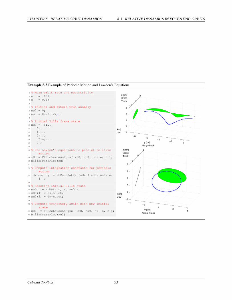
CHAPTER 8. RELATIVE ORBIT DYNAMICS 8.3. RELATIVE DYNAMICS IN ECCENTRIC ORBITS

Example 8.3 Example of Periodic Motion and Lawden’s Equations

1 % Mean orbit rate and eccentricity2 n = .001;3 e = 0.1;4

5 % Initial and future true anomaly6 nu0 = 0;7 nu = 0:.01:2*pi;8

9 % Initial Hills-frame state10 xH0 = [1;...11 0;...12 1;...13 0;...14 -2*n;...15 0];16

17 % Use Lawden’s equations to predict relativemotion

18 xH = FFEccLawdensEqns( xH0, nu0, nu, e, n );19 HillsFramePlot(xH)20

21 % Compute integration constants for periodicmotion

22 [D, dx, dy] = FFEccDMatPeriodic( xH0, nu0, e,1 );

23

24 % Redefine initial Hills state25 nuDot = NuDot( n, e, nu0 );26 xH0(4) = dx*nuDot;27 xH0(5) = dy*nuDot;28

29 % Compute trajectory again with new initialstate

30 xH2 = FFEccLawdensEqns( xH0, nu0, nu, e, n );31 HillsFramePlot(xH2)

−1

0

1

2

3

−8−6

−4−2

0

−2

0

2

y [km]Along−Track

z [km]Cross−Track

x [km]Radial

−2

−1

0

1

2

3

−4−2

02

4

−2

0

2

y [km]Along−Track

z [km]Cross−Track

x [km]Radial

CubeSat Toolbox 53

8.3. RELATIVE DYNAMICS IN ECCENTRIC ORBITS CHAPTER 8. RELATIVE ORBIT DYNAMICS

CubeSat Toolbox 54

INDEX

AddAxes, 23AnimationGUI, 41AnimQ, 18AntennaPatch, 21AtmDens2, 19AtmJ70, 36AttitudeProfileDemo, 39

BatterySizing, 42

C2DZOH, 7, 21CAD, 21coordinate transformation, 20cross, 26CubeSatAero, 38CubeSatFaces, 35CubeSatGGStabilized, 36CubeSatModel, 34, 35CubeSatPropulsion, 42CubeSatRadiationPressure, 38CubeSatRHS, 35CubeSatRWASimulation, 36CubeSatSimulation, 36

Date2JD, 19DemoPSS, 2, 13DesignMagneticTorquer, 42DrawSpacecraftInOrbit.m, 40

EarthRot, 18ECIToEF, 29ephemeris, 22Eul2Mat, 25Eul2Q, 26Euler angle, 26

FFSimDemo, 36FileHelp, 10Finder, 12, 14

GroundTrack, 40

Hall thruster, 21HallThrusterModel, 21help, 3

InterpolateState, 31IsothermalCubeSatDemo, 42

JD2Date, 23JPLPlanetDemo, 32Julian Date, 23

Kepler’s Equation, 20

LinkOrbitAnalysis, 42

MarsRot, 27Mat2Eul, 25MoonRot, 27MoonV1, 29MoonV2, 29

ObservationTimeWindows, 39ObservationTimeWindowsPlot, 39OrbitAndSensorConeAnimation.m, 41

PackageOrbitDataForPlayback, 41PID3Axis, 36PIDMIMO, 36PlanetPosition, 29, 30PlanetPosJPL, 30, 32Planets, 29PlaybackOrbitSim, 41Plot2D, 23Plot3D, 23PlotOrbit, 40PlotOrbitPage, 23PSSSetPaths, 2

Q2Eul, 26Q2Mat, 26QForm, 20, 26QLVLH, 20, 27QMult, 26QNadirPoint, 27QPose, 26QSunNadir, 27QTForm, 26quaternion, 20, 26QZero, 26

55

INDEX INDEX

RapidSwath, 39RBModel, 22RVFromKepler, 20

selenographic latitude, 27selenographic longitude, 27SkewSymm, 26solar flux, 22SolarCellPower, 35SolarFlx, 22SolarSys, 29, 30SolarSysJPL, 30, 32SunV1, 22, 29SunV2, 23, 29SunVectorECI, 29

TEarth, 29TEclipse, 29time, 23TPlanets, 29TwoSpacecraftOrbitSimulation, 36TwoSpacecraftSimpleOrbitSimulation, 36

CubeSat Toolbox 56