cur 412: game theory and its applications, lecture 4

CUR 412: Game Theory and its Applications,Lecture 4

Prof. Ronaldo CARPIO

March 22, 2015

Prof. Ronaldo CARPIO CUR 412: Game Theory and its Applications, Lecture 4

Homework #1

▸ Homework #1 will be due at the end of class today.

▸ Please check the website later today for the solutions to HW1 andHW2, which is due on 4/5.


Review of Last Lecture

▸ Last week, we looked at a classic application of game theory ineconomics: the behavior of oligopolies.

▸ In Cournot oligopoly, firms choose their quantity of output.

▸ Nash equilibrium outcome: firms split the market. Output andprofits are in between the case of monopoly and perfect competition.

▸ In Bertrand oligopoly, firms choose their price. Consumers only buyfrom the lowest price seller.

▸ Nash equilibrium outcome: firms set P =MC , make zero profit.Same as perfect competition.


Hotelling’s Model of Electoral Competition

▸ This is a widely used model in political science and industrialorganization, Hotelling’s ”linear city” model.

▸ Players choose a location on a line; payoffs are determined byhow much of the line is closer to them than other players.

▸ Here, location represents a position on a one-dimensionalpolitical spectrum, but it can also represent physical space orproduct space.


Location on Political Spectrum

xmin

v1

xmax

v2 v3 v4 v5

m

▸ Political position is measured by position on an interval ofnumbers

▸ xmin is the most ”left-wing” position, xmax is the most”right-wing” position

▸ Voters are located at fixed positions somewhere on the line.This position represents their ”favorite position”.

▸ In this example, there are five voters with favorite positions atv1...v5.

▸ The median position m is the position such that half of votersare to the left or equal to m, and the other half are to theright or equal to m.

▸ Voters dislike positions that are farther away from them onthe line. They are indifferent between positions to their leftand right that have the same distance.


Attracting Voters Based on Position

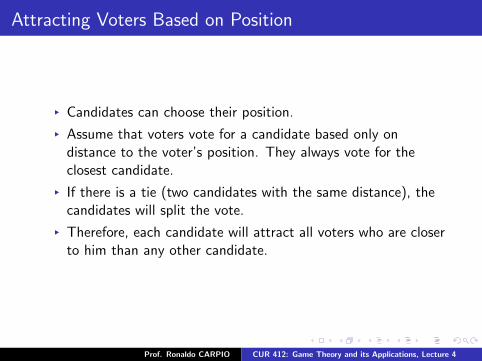
▸ Candidates can choose their position.

▸ Assume that voters vote for a candidate based only ondistance to the voter’s position. They always vote for theclosest candidate.

▸ If there is a tie (two candidates with the same distance), thecandidates will split the vote.

▸ Therefore, each candidate will attract all voters who are closerto him than any other candidate.


Attracting Voters Based on Position

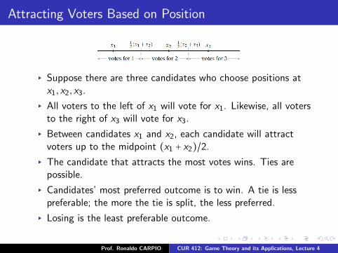
▸ Suppose there are three candidates who choose positions atx1, x2, x3.

▸ All voters to the left of x1 will vote for x1. Likewise, all votersto the right of x3 will vote for x3.

▸ Between candidates x1 and x2, each candidate will attractvoters up to the midpoint (x1 + x2)/2.

▸ The candidate that attracts the most votes wins. Ties arepossible.

▸ Candidates’ most preferred outcome is to win. A tie is lesspreferable; the more the tie is split, the less preferred.

▸ Losing is the least preferable outcome.


Candidates’ Payoff Function

▸ Payoffs can be represented by this function:

ui(x1, ...xn) =

⎧⎪⎪⎪⎪⎨⎪⎪⎪⎪⎩

n if candidate wins

k if candidate ties with n − k other candidates

0 if candidate loses

▸ Definition of Hotelling’s Game of Electoral Competition:▸ Players: the candidates▸ Actions: each candidate can choose a position (a number) on

the line▸ Preferences: Each candidate’s payoff is given by the function

above.


Let’s Play the 2-Person Game

▸ Assume voters (or consumers) are uniformly distributed alonga line that begins at 0 and ends at 100.

▸ I will choose 2 players.

▸ Each player will write down a number from 0 to 100. This istheir position on the line.

▸ Calculate the portion of the line that is closer to each player.

▸ The player with the larger portion wins (if portions are equal,there is a tie).


Two Candidates

▸ Suppose there are two candidates that choose positions x1, x2.

▸ The median position (half of voters are on the left, half on theright) is m.

▸ Let’s examine the best response function of player 1 to x2.

▸ Case 1: x2 < m▸ Player 1 wins if x1 > x2 and (x1 + x2)/2 < m. Every position

between xj and 2m − xj is a best response.

▸ Case 2: x2 > m▸ By the same reasoning, every position between 2m − xj and xj

is a best response.

▸ Case 3: x2 = m▸ Choosing m results in a tie; any other choice results in a loss.

Therefore, x1 = m is the best response.


Best Response Function

▸ Best response function is:

B1(x2) =

⎧⎪⎪⎪⎪⎨⎪⎪⎪⎪⎩

{x1 ∶ x2 < x1 < 2m − x2} if x2 < m

{m} if x2 = m

{x1 ∶ 2m − x2 < x1 < x2} if x2 > m

▸ Unique Nash equilibrium is when both candidates choose m.


Direct Argument for Nash Equilibrium

▸ At (m,m), any deviation results in a loss.▸ At any other position:

▸ If one candidate loses, he can get a better payoff by switchingto m.

▸ If there is a tie, either candidate can get a better payoff byswitching to m.


Implications of Equilibrium

▸ Conclusion: competition between candidates drives them totake similar positions at the median favorite position of voters

▸ In physical or product space: competing firms are driven tolocate at the same position, or offer similar products

▸ This is known as ”Hotelling’s Law” or ”principle of minimumdifferentiation”

▸ Requires the one-dimensional assumption on voter/consumerpreferences.

▸ If there is more than one dimension (e.g. consumers careabout both price and quality), this result may not hold


War of Attrition

▸ This game was originally developed as a model of animal conflict.

▸ Two animals are fighting over prey.

▸ Each animal gets a payoff from getting the prey, but fighting iscostly.

▸ Each animal chooses a time at which it will give up fighting; thefirst one to give up loses the prey.

▸ This can be applied to any kind of dispute between parties, wherethere is some cost to waiting.


Setup of the Game

▸ Two players are disputing an object. The player that concedes firstloses the object to the other player.

▸ Time is a continuous variable that begins at 0, goes on indefinitely.

▸ Assume that player i places value vi on the object (may be differentfrom other player’s value).

▸ If player i wins the dispute, he gains vi in payoff.

▸ Time is costly. For each unit of time that passes before one sideconcedes, both players lose 1 in payoff.


Payoffs

▸ Suppose that player i concedes first at time ti .

▸ Player i ’s payoff: −ti▸ Player j ’s payoff: vj − ti

▸ If both players concede at the same time, they split the object.

▸ Player i ’s payoff: vi/2 − ti▸ Player j ’s payoff: vj/2 − ti


Let’s play War of Attrition

▸ I will choose 2 players, with valuations of 5 and 10.

▸ Each player will write down a number ti ≥ 0. Reveal themsimultaneously.

▸ Suppose that ti < tj .

▸ Player i ’s payoff: −ti▸ Player j ’s payoff: vj − ti

▸ If ti = tj , they split the object.

▸ Player i ’s payoff: vi/2 − ti▸ Player j ’s payoff: vj/2 − ti


Definition of the Game

▸ Players: two parties in a dispute.

▸ Actions: each player’s set of actions is the set of concession times(a non-negative number).

▸ Preferences: Payoffs are given by the following function:

ui(t1, t2) =

⎧⎪⎪⎪⎪⎨⎪⎪⎪⎪⎩

−ti if ti < tj

vi/2 − ti if ti = tj

vi − tj if ti > tj



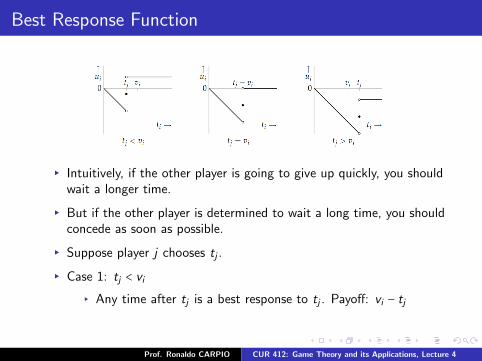
▸ Intuitively, if the other player is going to give up quickly, you shouldwait a longer time.

▸ But if the other player is determined to wait a long time, you shouldconcede as soon as possible.

▸ Suppose player j chooses tj .

▸ Case 1: tj < vi

▸ Any time after tj is a best response to tj . Payoff: vi − tj



▸ Case 1: tj < vi

▸ Any time after tj is a best response to tj . Payoff: vi − tj

▸ Case 2: tj = vi

▸ Any time after or equal to vi is a best response. Payoff: 0

▸ Case 3: tj > vi

▸ ti = 0 is the best response. Payoff: 0


Nash Equilibrium

▸ (t1, t2) is a Nash equilibrium if and only if:

▸ t1 = 0, t2 ≥ v1 or

▸ t2 = 0, t1 ≥ v2


Implications of Equilibrium

▸ Players don’t actually fight in equilibrium.

▸ Either player can concede first, even if he has the higher valuation.

▸ Equilibria are asymmetric: each player chooses a different action,even if they have the same value

▸ This can only be a stable social norm if players come from differentpopulations (e.g. owners always concede, challengers always wait)


Let’s Hold an Auction

▸ I will auction off 50 yuan.

▸ If you want to submit a bid, write down your ID number and bid (anumber ≥ 0) on the piece of paper.

▸ I will pay the difference between 50 and the highest bid. (If it isnegative, then the winner should pay me.)

▸ If there is a tie, the difference will be evenly divided among everyonewith the highest bid.

▸ What do you predict the outcome will be?



▸ This type of auction is called a first-price, sealed-bid auction.

▸ first-price, because the winner (the highest bidder) pays his bid▸ sealed-bid, because bids are made secretly, then revealed

simultaneously

▸ Also a type of common-value auction, since the value of the prize isthe same to all players

▸ What are the Nash equilibria of this auction?



▸ What are the Nash equilibria of this auction?

▸ Assume two players who bid x1, x2. The value of the prize is V .

▸ Let’s find Player 1’s best response to x2.

▸ Suppose x2 < V .

▸ No matter what x1 is, Player 1 can always improve his payoffby choosing a number closer to, and greater than, x2.

▸ No best response exists.

▸ Suppose x2 > V .

▸ Any number less than x2 gives the same payoff of 0. This isthe set of best responses.

▸ Suppose x2 = V .

▸ Any number ≤ V gives the same payoff of 0. This is the set ofbest responses.

▸ x1 = V , x2 = V is the only Nash equilibrium.



▸ Outcome is similar to Bertrand duopoly.

▸ Two players are enough to compete profits away to zero.


Auctions

▸ A good is sold to the party who submits the highest bid.

▸ A common form of auction:

▸ Potential buyers sequentially submit bids.

▸ Each bid must be higher than the previous one.

▸ When no one wants to submit a higher bid, the current highestbidder wins.

▸ The actual winning bid has to only be slightly higher than thesecond-highest bid.

▸ We can model this as a second-price auction: the winner is thehighest bidder, but only has to pay the second-highest price.


Second-price, sealed-bid auction

▸ Assume that each person knows his valuation of the object beforethe auction begins, so that valuation cannot be changed by seeinghow others behave.

▸ Therefore, there is no difference if all bids are made secretly, thensimultaneously revealed: a closed-bid auction.

▸ Each player submits the maximum amount he is willing to pay.

▸ The highest bidder wins, and pays the second-highest price.


Setup of the Game

▸ There are n bidders.

▸ Bidder i has valuation vi for the object. Assume that we label thebidders in decreasing order:

▸ v1 > v2 > ... > vn

▸ Each player submits a sealed bid bi .

▸ If player i ’s bid is the highest, he wins and has to pay thesecond-highest bid bj . Payoff: vi − bj

▸ Otherwise, does not win. Payoff: 0

▸ To break ties, assume player with the highest valuation wins.


Let’s Hold a Second-Price Auction

▸ I will choose 2 players. Each player will draw a card, which is either5 or 8. This will be your valuation of the prize.

▸ We will reveal everyone’s valuation.

▸ The players will write down their bids (a number ≥ 0) on a piece ofpaper.

▸ The highest bidder wins the prize, and pays the second-highest price.

▸ We will calculate everyone’s payoff.


Nash Equilibrium with 2 Players

▸ Suppose there are 2 players with valuations v1, v2. Assume v1 > v2.

▸ Each player bids bi .

▸ If b1 > b2, Player 1’s payoff is v1 − b2, Player 2’s payoff is 0.▸ If b2 > b1, Player 1’s 0, Player 2’s payoff is v2 − b1.▸ If b1 = b2, Player 1’s payoff is v1 − b1, Player 2’s payoff is 0.


Best Response Function with 2 Players

▸ Let’s find Player 1’s best response function.

▸ If b2 < v1, Player 1 can get a positive payoff by bidding b1 ≥ b2.Best response is b1 ≥ b2.

▸ If b2 = v1, Player 1 will get a zero payoff with any bid. Bestresponse is b1 ≥ 0.

▸ If b2 > v1, Player 1 can get a zero payoff by bidding b1 < b2, ora negative payoff if b1 ≥ b2. Best response is b1 < b2.

▸ Player 2:

▸ If b1 < v2, Player 2 can get a positive payoff by bidding b2 > b1.Best response is b2 > b1.

▸ If b1 = v2, Player 2 will get a zero payoff with any bid. Bestresponse is b2 ≥ 0.

▸ If b1 > v2, Player 2 can get a zero payoff by bidding b2 ≤ b1, ora negative payoff if b2 > b1. Best response is b2 ≤ b1.


Nash Equilibrium With More Than 2 Players

▸ If there are more than 2 players, best response function becomesvery complicated.

▸ There are many Nash equilibria in this game. Let’s examine somespecial cases.


All Players Bid their Valuation

▸ (b1...bn) = (v1...vn), i.e. every player’s bid is equal to his valuation.

▸ Player 1, who has the highest valuation, wins the object and pays v2.

▸ Player 1’s payoff: v1 − v2 > 0, all other players: 0

▸ Does anyone have an incentive to deviate?

▸ Player 1:

▸ If Player 1 changes bid to ≥ b2, outcome does not change▸ If Player 1 changes bid to < b2, does not win, gets lower payoff

of 0

▸ Players 2 ... n:

▸ If Player i lowers bid, still loses.▸ If Player i raises bid to above b1 = v1, wins, but gets negative

payoff vi − v1 < 0


Player 1 Bids Valuation, All Others Bid 0

▸ (b1...bn) = (v1,0...0), i.e. all players except player 1 bids 0

▸ Player 1 wins, pays 0. Payoff: v1

▸ Does anyone have an incentive to deviate?

▸ Player 1:

▸ Any change in bid results in same outcome (because oftie-breaking rules)


▸ If Player i raises bid to ≤ v1, still loses▸ If Player i raises bid to > v1, wins, but gets negative payoffvi − v1

▸ This outcome is better off for player 1, but worse off for the seller ofthe object


An Equilibrium where Player 1 Doesn’t Win

▸ (b1...bn) = (v2, v1,0, ...0). Player 2 wins the auction and pays pricev2. All players get a payoff of 0.

▸ Player 1:

▸ If he raises bid to x < v1, still loses.▸ If he raises bid to x ≥ v1 he wins, gets payoff of 0

▸ Player 2:

▸ If he raises bid or lowers to x > v2, outcome unchanged▸ If he lowers bid to x ≤ v2, loses auction, gets payoff of 0


▸ If he raises bid to x ≤ v1, still loses▸ If he raises bid to > v1, wins, but gets negative payoff vi − v1


An Equilibrium where Player 1 Doesn’t Win

▸ (b1...bn) = (v2, v1,0, ...0). Player 2 wins the auction and pays pricev2. All players get a payoff of 0.

▸ Player 2’s bid in this equilibrium exceeds his valuation.

▸ This seems risky - what if player 1 decided to bid higher than v2?

▸ In a dynamic setting, player 2’s bid is not credible.

▸ Later on, we’ll study ways of showing that these kinds of outcomesare implausible.


Equilibria with Weakly Dominant Actions

▸ For each player i , the action vi weakly dominates all other actions

▸ Player i can do no better than bidding vi , no matter what otherplayers bid

▸ If the highest bid of other players is ≥ vi , then:

▸ If player i bids vi , payoff is 0 (either win and pay vi , or don’twin)

▸ If player i bids bi ≠ vi , payoff is zero or negative

▸ If the highest bid of the other players is b < vi , then:

▸ If player i bids vi , wins and gets payoff vi − b▸ If player i bids bi ≠ vi , either wins and gets same payoff, or

loses and gets payoff of 0

▸ Second-price auction has many Nash equilibria, but the onlyequilibrium where each player plays a weakly dominant action is(b1...bn) = (v1...vn).


First-price, sealed bid auction with n players

▸ We saw that in the first-price sealed bid auction with 2 players whohad the same valuation, the only NE was (b1,b2) = (v1, v2).

▸ Now, let’s allow n players, and valuations can differ among players.

▸ Assume that if there is a tie, the winner is the player with thehighest valuation.

▸ First, let’s check the obvious case, where everyone bids theirvaluations: (b1...bn) = (v1...vn)

▸ The winner, Player 1, has an incentive to deviate: he can increasehis payoff by lowering his bid from v1 to v2.

▸ Note that this results in the same payoffs as the second-priceauction.


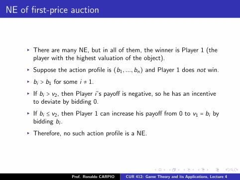
NE of first-price auction

▸ There are many NE, but in all of them, the winner is Player 1 (theplayer with the highest valuation of the object).

▸ Suppose the action profile is (b1, ...,bn) and Player 1 does not win.

▸ bi > b1 for some i ≠ 1.

▸ If bi > v2, then Player i ’s payoff is negative, so he has an incentiveto deviate by bidding 0.

▸ If bi ≤ v2, then Player 1 can increase his payoff from 0 to v1 = bi bybidding bi .

▸ Therefore, no such action profile is a NE.


Review of Random Variables

▸ A random variable is a variable that can take on different values,according to some probability distribution.

▸ A finite, discrete random variable is random variable that can takeon a finite number of values.

▸ For example, suppose that y is a random variable that can take ontwo values:

▸ y = 1 occurs with probability p,▸ y = 0 occurs with probability 1 − p.

▸ y can represent the outcome of flipping a biased coin that shows 1on one side and 0 on the other side.

▸ If we flip this coin a very large number of times, the frequency (i.e.the fraction of flips) of showing 1 will be p.


Expected Values

▸ The expected value of a random variable is the weighted sum of allpossible outcomes, weighted by the probability of occurrence.

▸ For the biased coin example, the expected value is:

E(y) = Pr(y = 1) ⋅ 1 + Pr(y = 0) ⋅ 0

= p ⋅ 1 + (1 − p) ⋅ 0

= p

▸ In general, the expected value (EV) of a discrete random variablethat can take on n outcomes y1, ...yn with probabilities p1, ...pn is

E(y) = p1y1 + p2y2 + ... + pnyn

▸ The sum of probabilities over all outcomes must add up to 1.


Next Lecture & Homework

▸ Homework #1 will be due at the end of class today.

▸ Please check the website later today for the solutions to HW1 andHW2, which is due on 4/5.

▸ For next week, please read Chapter 4.


cur 412: game theory and its applications, lecture 4

Documents