curriculum choice, educational performance, and …

STUDY PAPER 124 FEBRUARY 2018

CURRICULUM CHOICE, EDUCATIONAL PERFORMANCE,AND WAGES WITHIN STEM

LENE KROMANN, ANDERS SØRENSEN AND JEANETTE WALLDORF

Curriculum choice, educational performance, and wages within STEM

Copenhagen 2018

Lene Kromann, Anders Sørensen and Jeanette Walldorf

The ROCKWOOL Foundation Research Unit

Study Paper No. 124

Curriculum choice, educational performance, and wages within STEM

Study Paper 124

Published by:© The ROCKWOOL Foundation Research Unit

Address:The ROCKWOOL Foundation Research UnitSoelvgade 10, 2.tv.DK-1307 Copenhagen K

Telephone +45 33 34 48 00E-mail: [email protected] site: www.rockwoolfonden.dk/en

Commissioned at University Press of Southern Denmark.

Price: 49 DKK including VAT.

February 2018

Contents

1 Introduction . . . . . . . . . . . . . . . . . . . . . . . . . . . . . . . . . . . . . . . . . . . . . . . . . 6

2 Literature . . . . . . . . . . . . . . . . . . . . . . . . . . . . . . . . . . . . . . . . . . . . . . . . . . . 8

3 Data and Institutional Setting . . . . . . . . . . . . . . . . . . . . . . . . . . . . . . . . . . . 103 .1 The sample . . . . . . . . . . . . . . . . . . . . . . . . . . . . . . . . . . . . . . . . . . . . . . . 103.2 STEM-classification . . . . . . . . . . . . . . . . . . . . . . . . . . . . . . . . . . . . . . . 113 .3 Descriptive Statistics . . . . . . . . . . . . . . . . . . . . . . . . . . . . . . . . . . . . . . . . 13

4 The Correlation Study . . . . . . . . . . . . . . . . . . . . . . . . . . . . . . . . . . . . . . . . . 174 .1 The empirical model . . . . . . . . . . . . . . . . . . . . . . . . . . . . . . . . . . . . . . . 174 .2 Results . . . . . . . . . . . . . . . . . . . . . . . . . . . . . . . . . . . . . . . . . . . . . . . . . . . 184 .3 Controlling for Relative Ability . . . . . . . . . . . . . . . . . . . . . . . . . . . . . . . 234 .4 Controlling for Industry Composition of Jobs . . . . . . . . . . . . . . . . . . . . 25

5 Conclusion . . . . . . . . . . . . . . . . . . . . . . . . . . . . . . . . . . . . . . . . . . . . . . . . . . 28

6 References . . . . . . . . . . . . . . . . . . . . . . . . . . . . . . . . . . . . . . . . . . . . . . . . . . . 29

7 Appendix . . . . . . . . . . . . . . . . . . . . . . . . . . . . . . . . . . . . . . . . . . . . . . . . . . . 31

5

Abstract

The importance of curriculum choice for subsequent income is studied, using de-tailed education data from the Master of Science in Engineering program at the Technical University of Denmark (DTU). It is found that there are large differences across areas of specialization within STEM . Compared to graduates specialized in Science (S), graduates specialized in Mathematics (M) have a starting wage that is 20 percent higher, and graduates specialized in Technology (T) have a starting wage that is approximately 15 percent higher; graduates specialized in Engineering (E) have a similar starting wage. Wage variation within the specific education program is of comparable importance to the wage variations between broad types and different lengths of education . Moreover, large variations in wages exist within the four STEM areas, which can be partly explained by course choice. Specifically, courses in M are associated with higher wages in most areas of specialization, which indicates that M is a general-purpose skill . In contrast, S, T and E are to a higher extent specific-purpose skills, as courses in these fields are not associated with higher wages if completed outside the area of specialization. In addition, a higher GPA obtained in the specific program is associated with higher wages. Approximately half of the wage differences can be explained by the industry composition of jobs . Proxies for individual ability, in the form of the course taken and the average GPA from high school, are included in the regressions to control for individual ability .

76

1 Introduction

This paper studies the following question: How important is curriculum choice in a higher education program for a student’s subsequent career? This is important to understanding how further education affects the creation of human capital. Is the curriculum choice within specific educational programs important, or is the return on education affected more by educational type (natural science, social science, business administration, etc .) and length (high school, bachelor’s, master’s, etc .)? There is limited knowledge about this issue .

The importance of curriculum choice for starting income is studied for candidates in the Master of Science in Engineering program at the Technical University of Denmark (DTU) . The main reason for selecting this program is that STEM is often claimed to be important for productivity and economic growth . A number of mod-els of economic growth emphasize the importance of engineers for innovation and R&D; see, for example, Romer (1990) . Knowledge of the importance of STEM qualifications and more specific qualifications within STEM – for example, within Science (S) – for individual productivity as measured by wages is, however, limited and is the focus of this study. To our knowledge, the present study is the first to ex-amine in detail the relationship between STEM qualifications and starting salaries within a specific graduate program.

We run wage regressions including, among others, information on course selec-tion and the GPA obtained in the program . The main result is that wage variation within the specific educational program is of quantitative importance. For exam-ple, graduates who specialize in M, i.e., take most courses within the field, have on average a starting salary that is 20 percent higher than graduates specialized in S . Graduates who fully specialize in M, i.e., take all their courses within the field, have on average a starting salary that is 27 percent higher than graduates who are fully specialized in S .

Moreover, coursework in M enters positively and significantly in four out of five ar-eas of specialization . In other words, M is correlated with higher wages in (almost) all specializations and can be interpreted as a general-purpose skill . On the other hand, S, T, and E are not correlated significantly with income when coursework is com-pleted outside the area of specialization. For example, graduates specialized in T do not have higher wages if they take courses in S or E . This suggests that S, T, and E can be interpreted as specific-purpose skills .

7

Wage variation within the specific education program is of comparable magnitude to wage variations between type and length of education. For comparison, Dal-gaard et al. (2009) find that a degree in the humanities in Denmark is associated with 22 percent lower earnings compared to a non-humanities degree; Iversen et al. (2016) find a wage gap of 40 percent between employees with upper secondary degrees and higher education .1 This indicates that curriculum choice within specific graduate programs is potentially very important for graduates’ productivity and has a magnitude that matches both type and length of education .

The analysis is made possible by a dataset on engineering graduates from DTU . Specifically, the dataset contains information on the curriculum choices and grades obtained . The dataset is linked with register data from Statistics Denmark, which contains information on the individuals’ labor market history . In addition, the da-taset includes information on graduates’ educational history prior to the master’s education, as well as information about their parents’ education and income .

A limitation of the analysis is that the estimated effects may be subject to omitted variable bias. The concern is related to variation in individual ability. For example, if individuals who are highly skilled in mathematics specialize in mathematical courses, and if this specialization subsequently results in higher wages, we cannot rule out the possibility that ability, not curriculum choice, is what results in higher wages. To handle this challenge, we include proxies for ability – measured by aver-age GPA in high school, courses selected in high school and other educational in-formation – in the analysis. It is found that the presented results are robust against the inclusion of such proxies . Despite this, we cannot rule out the possibility that unobserved factors are important, as we may not have controlled sufficiently for individuals’ ability . In that sense, the analysis presented is a correlation study rather than a study of causality . Nevertheless, we consider the analysis to be of interest because there exist only a few studies on curriculum choice and wages and no study focusing on STEM .

The remainder of the paper is organized as follows: In section 2, previous studies are presented . In section 3, the data and institutional setting are introduced, and section 4 presents the results . Section 5 concludes .

1 The economic literature shows that the wage gap between college majors is of the same magnitude as the wage gap between high school and college (Altonji, 2012; Kirkeboen et al ., 2016) .

98

2 Literature

Few studies have investigated the variation within higher education programs in the return on education . Three studies focus on highly selected individuals from top US schools, and one study analyzes a higher education program at Copenhagen Business School . All these studies focus on education programs within the social sciences and business economics . Athey et al . (2007) study graduate students from the five highest-ranked economics Ph.D. programs in 1993 (Harvard University, MIT, Princeton University, Stanford University, and the University of Chicago) and find that first-year grades in mandatory courses are a strong predictor of economics graduate students’ job placements, but they do not examine how different courses impact job placements . Bertrand et al . (2010) examine the salary gap between male and female MBA students from Chicago Booth (the business school of the Univer-sity of Chicago). They find that men take more finance courses and have higher GPAs; the GPA, however, has no impact on wages, whereas the share of finance courses of all courses taken is significantly positively related to wages. Lazear (2012) studies MBAs from the Stanford Graduate School of Business (the business school of Stanford University) and uses three variables to describe differences in course plans; these are the number of economics courses taken, the number of finance courses taken, and the maximum number of courses taken within one field. Only the number of finance courses has a significant positive impact on wages.

Dahl et al . (2016) use detailed educational data on graduates from Copenhagen Business School. They find that choosing courses in management is a significant predictor of leadership and that individuals who have diversified curricula, with many different types of classic business courses, are more likely to become manag-ers. By contrast, they found that educational diversification outside classic business courses is not significant in the model. The paper also finds that courses in manage-ment, marketing, finance and accounting show a positive correlation with wages.

Carnevale et al. (2015) study wage differences at the bachelor’s level but do not link wage differences to the selection of courses. It is found that there are large wage gaps both between and within 15 bachelor’s degree areas. For example, stu-dents with a major within STEM have the highest starting wages and experience the highest wage increases during their careers, compared to non-STEM students . Within STEM, the starting salary is highest for engineers (median of $50,000), followed by mathematicians (median of $43,000) . The two lowest-earning STEM groups earn less than the median annual wage of college-educated workers

9

($33,000) . It is concluded that there is a large variation in salaries both within and between STEM majors in the US .

Several studies more generally compare wages between educational types . Blundell et al . (2000) use the UK National Child Development Study, with information on family background for children born in a specific week in March 1958, their ed-ucational choices, and labor market data on hourly wages . They use the salary in 1991, when the individuals were 33 years old . Estimation is performed using match-ing, where people with higher education are compared to people who could have completed higher education but chose not to do so . In accordance with previous studies, Blundell et al. (2000) find significant differentials. For example, chemistry and biology achieve the lowest return on education, while economics, accounting and law gain the highest return. Another study focusing on differences between majors is Arcidiacono (2004), who similarly finds large differences in wages between majors, such as the natural sciences, business administration, the social sciences, the humanities, etc .

1110

3 Data and Institutional Setting

The backbone of the analysis is a dataset from the DTU . The dataset contains the full exam transcripts for all engineers graduating from DTU since 1996 . The data-set is linked to the Danish matched employer-employee dataset, which gives access to information on wages and other labor market variables . Moreover, the dataset is linked to graduates’ pre-tertiary educational performance, as well as personal and parental background characteristics .

3.1 The sample

The data from DTU covers a period from 1996 to 2016 . To avoid the possibility that changes in the institutional setup at DTU would influence the results, a period with only minor changes in the study structure is selected . In addition, to follow graduate engineers for up to 10 years on the labor market, an early period is pri-oritized . This results in a sample of students who were admitted to DTU in the 2003/2004 study year or earlier and who started a general 5-year program (civil engineering) . The sample is limited to students who started completion of the last 120 European Credit Transfer and Accumulation System (ECTS)2 credits in the fall term of 1997 or later3. The final sample for analysis includes approximately 3,500 individuals who graduated from the 5-year program .

The chosen program is characterized by few rules and regulations, allowing students to freely choose from all available courses . The study guidebook from 2003/2004 states that students complete approximately 35 courses, 3-5 courses per semester. In the first four semesters, they face one restriction, which is successful completion of a specific compulsory course program.4 Since the first part of the degree program is partly mandatory, the last two academic years of the program are used in this analysis . In this part of the program, the individual specialization is expected to be most pronounced . More precisely, the analysis is limited to the

2 ECTS credits measure the quantity of further education in the European Union. For successfully completed studies, ECTS credits are awarded . One academic year corresponds to 60 ECTS credits .3 This restriction is because of a data break since significant changes were made to the supply of courses and the naming of courses in 1997 .4 The main elements of the compulsory course program were an introduction to the core of mathematics, physics and chemistry (adapted to the individual compulsory course program), an introduction to the field’s technical courses, and a project focusing on interdisciplinary skills . It is important to note that the compulsory course program did not lock students’ further study opportunities .

11

last 120 ECTS credits of the engineering degree . This is generally the last four semesters of the 5-year degree and corresponds to a master’s degree following the Bologna Declaration . During the last two years, students choose 3 to 5 courses per semester from approximately 700 courses offered annually.

3.2 STEM-classification

This section describes the applied course classification of the analysis. To reduce the dimensions in curriculum choice, courses are divided into five areas: Science (S), Technology (T), Engineering (E), Mathematics (M) and Management (L) .

There is a very large supply of courses at DTU, and the 3,500 students in the sam-ple passed approximately 1,600 of these within the last 2 years of their studies .5 On average, a course has been taken by 33 of the students in the sample . However, per semester, a course was taken by an average of only 5 .8 students; for 50 percent of the courses, there were 3 or fewer students in the sample . This indicates that stu-dents in our sample have very different course curricula in the final two years of their graduate studies . A student typically takes 13 courses in the last 2 years; the remaining credits are obtained through projects, including a final thesis.

The large variation in courses is an advantage but also a challenge in the analysis of curriculum choices . On the one hand, it is a prerequisite for our analysis that there is a large degree of individual specialization . However, to make precise pre-dictions, a level of aggregation is needed . To reduce the data variation, courses are aggregated into the five groups. The reason for dividing courses into STEM is the great interest in STEM in many countries; see, for example, Romer (2001) .6 Thus, there seems to be general agreement that STEM is an important education type for individuals and the society at large. It is less clear which specific qualifications within STEM lead to higher productivity . Management is chosen as a specialization in addition to STEM because the structure at DTU makes it a natural area to sepa-rate out . In addition, high-quality management has been found to be important for

5 The 1,600 courses correspond to different choices from the DTU course database. Projects and the master’s thesis are not included in this .6 Romer (2001) points to a flaw in the US innovation strategy: ignoring the structure of the institution of higher education . An inelastic labor supply will lead investment in R&D to transform into higher wages instead of technological progress . Consequently, he argues that government programs focusing on the demand side that were intended to speed up technological processes had very little effect. Instead, the government should subsidize the supply in the market for scientists and engineers .

1312

firms’ performance (e.g., Bloom and Van Reenen, 2010), which makes a focus on management relevant .

The aggregation of courses into the 5 areas is performed using the department structure at DTU that offers courses more or less related to the different fields. Table 1 shows which departments we aggregate into the five areas.7 In addition, the percentage of students taking courses within the 5 areas and 14 departments is shown . By aggregating the courses into 5 areas, the analysis is more robust, yet an important part of the course variation remains in the data .8

Table 1. Departments and aggregation of courses into 5 areas

Areas Departments Share of students Average share

Science: S 0.55 0.20Physics 0.31 0.04Chemistry 0.22 0.04Systems Biology 0.18 0.08Micro- and Nanotechnology 0.09 0.03

Technology: T 0.72 0.26Chemical Engineering 0.17 0.04Electrical Engineering 0.37 0.08Photonics 0.17 0.04Mechanical Technology 0.26 0.08

Engineering: E 0.32 0.16Building and Construction 0.19 0.08Water and Environmental Technology 0.20 0.07

Mathematics: M 0.74 0.21Mathematics 0.25 0.02Informatics and Mathematical Modeling 0.69 0.18

Management: L 0.78 0.17Planning, Innovation and Management 0.77 0.15Transportation and Traffic 0.05 0.01

Source: Own calculations based on data from DTU and Statistics Denmark.

7 The students also had the opportunity to take courses at other educational institutions in Denmark or abroad . In addition, DTU offers language courses and other courses. These courses typically fall below 5 ECTS credits for the individual student and are not part of this analysis .8 It should be noted that the decision to reduce the variation in data and the use of departments naturally also defines some limitations of this study. Most of the departments at DTU could claim that they educate students in several qualifications across the chosen areas. This variation is excluded in this analysis.

13

All courses can naturally be classified as “engineering” as we analyze an engineer-ing program. The division in STEM areas should be understood as a classification within the field of engineering. E is chosen to represent a particular group of courses and is a narrower definition than overall engineering. The classic courses of engineering (building, electrical, machine and production) are divided into E and T, where T has a relatively higher industrial focus than E . S is chosen to rep-resent science (including courses such as physics, chemistry, and biology) . M and L cover courses offered by the Department of Mathematics and Department of In-formation and Mathematical Modeling, respectively, the Department of Planning, Innovation, and Management, and the Department for Transportation and Traffic. It appears that 78 percent of the sample took courses within Management and that 74 percent took courses within Mathematics . Conversely, only 32 percent took courses within Engineering .

3.3 Descriptive Statistics

In this section, the wage variation between and within the 5 areas is explored . In Figure 1, the cumulative distribution function for starting salary is presented by the 5 areas of specialization, where the area of specialization is defined as the area in which students obtained the highest number of ECTS credits . The median starting salary for specialization in M is around DKK 432,000, while the median starting salary for T and L is around DKK 409,000. Finally, the median starting salaries for E and S are around DKK 381,000 and 336,000, respectively . In other words, there is about a DKK 96,000 or 29 percent difference in the median annual starting sal-ary between individuals specialized in M and S . Eighty percent of individuals spe-cialized in M earn around DKK 350,000 or more, whereas only 45 percent earn that amount or more if specialized in S . In addition, variation within specialization areas is large; for instance, the middle 60 percent of individuals specialized in M, i .e ., individuals between the 20th and 80th percentile, earn between DKK 350,000 and 500,000. It is also apparent from the figure that M stochastically dominates the other 4 areas and that L and T stochastically dominate E and S .

In Table 2, the variations in courses across the 5 areas are presented . The table is best understood by focusing on one area of specialization at a time . In the following, we focus on T as the area of specialization . It appears from the second row of the table that 983 of the students have T as their area of specialization. For example, the top 10 percent of individuals within T have 91 percent or more of their ECTS credits within T, while the bottom 10 percent of individuals have only 54 percent

1514

or less of their ECTS credits within T . In addition to courses within T, 46 percent of the individuals have credits within S, 18 percent within E, 73 percent within M, and 75 percent within L . There is also a large spread in how many areas in which the students have taken courses, and how large a percentage of their credits they have in the different areas. For example, some students have more than 23 percent of their courses within L, and other students have more than 31 percent of their courses within M . In other words, there is a large variation in the course choice of individuals specialized within T . Similar patterns apply for the other four areas of specialization . This is reassuring since there are no restrictions on how the ed-ucation is structured across these program areas, and no obvious combinations of courses within the five areas of specialization are observed.

Table 2. Distribution of credits within the five areas of specialization

Science Technology Engineering Mathematics Management

Specialization Share p10 p90 Share p10 p90 Share p10 p90 Share p10 p90 Share p10 p90

S (n=743) 1 0.58 0.95 0.58 0.04 0.28 0.12 0.04 0.17 0.67 0.04 0.17 0.72 0.04 0.15

T (n=983) 0.46 0.04 0.27 1 0.54 0.91 0.18 0.04 0.29 0.73 0.04 0.31 0.75 0.04 0.23

E (n=619) 0.35 0.04 0.13 0.53 0.04 0.17 1 0.59 0.93 0.68 0.04 0.18 0.73 0.04 0.24

M (n=673) 0.51 0.04 0.14 0.69 0.04 0.35 0.08 0.04 0.29 1 0.56 0.93 0.77 0.04 0.21

L (n=507) 0.37 0.04 0.15 0.65 0.04 0.32 0.34 0.04 0.36 0.61 0.04 0.22 1 0.51 0.96

Note: The rows indicate the area a student has the most credits in (specialization), and the columns indicate the distribution of credits across the 5 areas. Share indicates the percentage of students who have credits in the area. P10 indicates the 10th percentile for students who have credits in the area. The P90 indicates the 90th percentile. As an example, the first cell (S, S) says that everyone with a primary focus in S has, by definition, courses within S. Eighty percent of students take 58 percent to 95 percent of their courses within S. Thus, 90 percent of students with S as their main area have more than 58 percent of their courses within S. The top 10 percent takes more than 95 percent of their courses within S.


Finally, in Figure 2, the average salaries across the 5 areas over time are present-ed .9 The figure confirms that, in the first job, the average wage gap is about DKK 100,000 between S and M, corresponding to 28 percent. This difference is persis-

9 The figure is based on an unbalanced sample with 3,525 engineers after 1 year, 2,055 engineers after 8 years and 1,302 engineers after 10 years. This is a consequence of how the sample was defined.

15

tent . However, two areas have stronger wage increments compared to the other areas . These are L and S . Individuals specialized in L start out being, on average, the third best-paid group, while individuals specialized in S on average begin as the lowest-paid group . After 10 years, however, L is on average the best-paid specializa-tion, while S is on average better paid than E .

In conclusion, large variations in starting salaries exist across and within the five areas. In the following section, the paper investigates whether these differences can be (partly) explained by differences in course choice. However, it is stressed that no causal identification strategy is used, and the analysis should be thought of as a correlation study rather than a study of causality . Nevertheless, the analysis is con-sidered to be of interest because there exist only a few studies on curriculum choice and wages, and no study focuses on STEM . In addition, it should be mentioned that we do include proxies to control for differences in individual ability.

Figure 1. Cumulative Wage Distribution by Specialization.

Percentiles are averages of 5 individuals around the specific percentile to fulfill Statistics Denmark’s rules on anonymity.


1716

Figure 2. Average Wage Income over Time (by Specialization).

Percentiles are averages of 5 individuals around the specific percentile to fulfill Statistics Denmark’s rules on anonymity.


17

4 The Correlation Study

In this section, wage regressions are used to investigate to what extent course choic-es are associated with differences in starting salaries.

4.1 The empirical model

We estimate the following wage regression:

10

4. TheCorrelationStudyInthissection,wageregressionsareusedtoinvestigatetowhatextentcoursechoicesareassociatedwithdifferencesinstartingsalaries.

4.1TheempiricalmodelWeestimatethefollowingwageregression:

𝑦𝑦" = 𝛽𝛽% + 𝛽𝛽'𝑍𝑍" + 𝛼𝛼'𝑋𝑋" + 𝜃𝜃,," + 𝜀𝜀",

where𝑦𝑦" measures(thelogarithmof)theannualsalaryforthefirstfullcalendaryearaftergraduation.𝑍𝑍" is a vector of variables describing individuals’ course choices;𝑋𝑋" is a vector of personal and parentalcharacteristicsthatisincludedtopartlycontrolforindividualabilitythatispotentiallycorrelatedwiththechoiceofcoursesandsubsequentlabormarketperformance.𝜃𝜃,," areyeardummiesthatequalonetheyearastudenthascompletedthedegree.Theyeardummiescontrolformacroeconomicshocksthatmayaffectsalariesandthelabormarketingeneral(seeKahn,2010;Oreopoulosetal.,2012).𝜀𝜀" isarobuststandarderror.Thecoefficientvector,𝛽𝛽,isthevectorofinterestthatdescribestheeffectofthecoursechoiceonstartingsalaries.

Inthefollowing,weapplythreeapproachestoincludinginformationonindividuals’coursechoices.First,𝑍𝑍" includesfourdummyvariables,oneforeachoftheareasofspecialization(usingSasthereferencegroup).Theresultsarepresented inTable3.Second,𝑍𝑍" includes fourcontinuousvariables (usingSasreference),with the sharesofECTScreditswithin the5areas inTable4.Thisapproachenablesus toanalyzecombinationsofcoursesacrossthe5areas.TheresultsarepresentedinTable4.Third,weusethefivesharesofECTScreditscombinedwitheachofthe5areasofspecialization.ThisisalessrestrictiveversionoftheapproachusedinTable4,astheimpactof,forexample,theshareofmathematicscourses,isallowedtovaryacrossareasofspecialization.Asaconsequence,𝑍𝑍" includes24variables(5x5,excludingthereferencegroup).TheresultsarepresentedinTable6.(ThestructureofTable6followsthatofTable2, i.e.,withineachofthefiveareasofspecialization,thesharesofECTScreditsacrossthe5areasareincluded).

4.2ResultsTable 3 presents coefficients from the wage regression for the first job and focuses on the area ofspecialization.Inthefirstcolumn,dummiesfortheareaofspecialization,GPAforthelast2yearsofthedegree, anddummies for graduationyearare includedas theonlyexplanatoryvariables. This followsFigure 1,with the difference that the table controls forGPA and the year of graduation. Specifically,dummiesareincludedforspecializationwithinT,E,MandL,whileSisusedasthereferencegroup.Thecoefficientsmeasure the salary gains for the corresponding area of specialization compared to beingspecializedinS. It isseenthatindividualswithinT,MandLreceiveonaverageahigherstartingsalarythan individualswithinS.ApersonspecializedwithinMhasonaveragethehigheststartingsalary,anaverageof20percenthigherthanS.10ForindividualsspecializedinTorL,thesalarygainisonaverage14

10Thepercentagedifferenceisequaltoexp(0.200)-1=22percent,whilethe0.20referstodifferencesinlogpoints.Inthefollowing,werefertotheestimatedcoefficientsaspercentagedifferences,althoughthisisonlyapproximatelycorrect.

where

10








measures (the logarithm of) the annual salary for the first full calendar year after graduation .

10








is a vector of variables describing individuals’ course choices;

10








is a vector of personal and parental characteristics that is included to partly control for individual ability that is potentially correlated with the choice of courses and subsequent labor market performance .

10








are year dummies that equal one the year a student has completed the degree . The year dummies control for macroe-conomic shocks that may affect salaries and the labor market in general (see Kahn, 2010; Oreopoulos et al ., 2012) .

10








is a robust standard error. The coefficient vector,

10








, is the vector of interest that describes the effect of the course choice on starting salaries .

In the following, we apply three approaches to including information on individuals’ course choices. First, includes four dummy variables, one for each of the areas of specialization (using S as the reference group) . The results are presented in Table 3 . Second, includes four continuous variables (using S as reference), with the shares of ECTS credits within the 5 areas in Table 4 . This approach enables us to analyze combinations of courses across the 5 areas . The results are presented in Table 4 . Third, we use the five shares of ECTS credits combined with each of the 5 areas of specialization . This is a less restrictive version of the approach used in Table 4, as the impact of, for example, the share of mathematics courses, is allowed to vary across areas of specialization . As a consequence, includes 24 variables (5x5, ex-cluding the reference group) . The results are presented in Table 6 . (The structure of Table 6 follows that of Table 2, i.e., within each of the five areas of specializa-tion, the shares of ECTS credits across the 5 areas are included) .

1918

4.2 Results

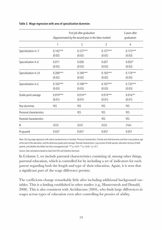
Table 3 presents coefficients from the wage regression for the first job and focuses on the area of specialization. In the first column, dummies for the area of spe-cialization, GPA for the last 2 years of the degree, and dummies for graduation year are included as the only explanatory variables. This follows Figure 1, with the difference that the table controls for GPA and the year of graduation. Specifically, dummies are included for specialization within T, E, M and L, while S is used as the reference group. The coefficients measure the salary gains for the corresponding area of specialization compared to being specialized in S . It is seen that individu-als within T, M and L receive on average a higher starting salary than individuals within S . A person specialized within M has on average the highest starting salary, an average of 20 percent higher than S .10 For individuals specialized in T or L, the salary gain is on average 14 percent and 11 percent, respectively, compared to indi-viduals specialized in S . Starting salaries in specialization areas S and E do not differ in a statistical sense . Moreover, a high university GPA is important to the starting salary . It is seen that an additional GPA point leads to a higher starting salary of approximately 2 percent; the Danish grade scale runs from the pass mark of 2 to the best mark of 12 .

Columns 1 through 3 include additional background information in

10








, reading from left to right . In Column 2, personal characteristics consist of, among other things, the high school GPA. We include this variable to control for the “absolute ability” of students. This GPA is a weighted average of the grades in the final exam in each course . The quality of the courses, as well as the GPA, is comparable across high schools since all students within the same cohort face identical written exams; all exams and major written assignments are evaluated by the student’s own teacher, as well as external examiners (teachers from other high schools) . The external examiners are assigned by the Danish Ministry of Education . In Column 2, two measures of student performance are included: the GPA from the master’s program and the GPA from high school . Including personal characteristics in the wage equation, the wage gap across areas of specialization narrows slightly, but the significant part of the difference persists.

10 The percentage difference is equal to exp(0.200) - 1 = 22 percent, while the 0.20 refers to differences in log points. In the following, we refer to the estimated coefficients as percentage differences, although this is only approximately correct .

19

Table 3. Wage regression with area of specialization dummies

First job after graduation (Approximated by the second year in the labor market)

5 years after graduation

1 2 3 4

Specialization in T 0.142*** 0.127*** 0.127*** 0.115***(0.02) (0.02) (0.02) (0.03)

Specialization in E 0.011 0.028 0.027 0.052*(0.03) (0.03) (0.03) (0.03)

Specialization in M 0.200*** 0.184*** 0.183*** 0.174***(0.02) (0.02) (0.02) (0.03)

Specialization in L 0.103*** 0.108*** 0.107*** 0.135***(0.03) (0.03) (0.03) (0.03)

Grade point average 0.019*** 0.014** 0.014*** 0.016**(0.01) (0.01) (0.01) (0.01)

Year dummies YES YES YES YES

Personal characteristics YES YES YES

Parental characteristics YES YES

N 3525 3525 3525 3165

R-squared 0.037 0.057 0.057 0.051

Note: OLS log-wage regression with robust standard errors in brackets. Personal characteristics: Female and child dummies and their cross-product, age at the start of the education, and the admission grade point average. Parental characteristics: Log-income of both parents, education dummy of both parents, and whether the father has had a management job. *** p <0.01, ** p <0.05, * p <0.1.


In Column 3, we include parental characteristics consisting of, among other things, parental education, which is controlled for by including a set of indicators for each parent regarding both the length and type of their education . Again, it is seen that a significant part of the wage difference persists.

The coefficients change remarkably little after including additional background var-iables. This is a finding established in other studies (e.g., Hamermesh and Donald, 2008). This is also consistent with Arcidiacono (2004), who finds large differences in wages across types of education even after controlling for proxies of ability .

2120

In Column 4, the salary is measured 5 years after graduation . It appears that wage differences are very persistent, which is consistent with the trends presented in Fig-ure 2 .

The results presented in Table 3 are estimated assuming that it is the area of spe-cialization only that is associated with starting salaries, limiting any effect of the degree of specialization . This assumption is relaxed in Table 4, where wage regres-sions are presented for the first job, focusing on course choices measured by share of ECTS credits within the 5 areas . Taking courses within M compared to S gives on average the largest salary gain . The results quantify that an individual who takes 10 percent of his ECTS credits in M and 90 percent in S earns on average 2 .71 per-cent more in the first job. Approximately 50 percent of individuals specialized with-in S take courses in M, and individuals take up to 46 percent of their credits within M. This implies that on average the yearly salary differences can be up to 12.5 per-cent, equivalent to approximately DKK 44,000 for individuals within S . Similarly, an individual with one third of his courses in each of the three areas T, M and L has a starting salary that is 20 percent (=0.184/3+0.272/3+0.148/3) higher than that of an individual fully specialized in S . If an individual takes all courses within M, he will have an average initial salary that is 27 .2 percent higher - equivalent to DKK 96,000 – compared to someone who has taken all his credits within S .

21

Table 4. Wage regression with credit shares independent of specialization


5 years after graduation

1 2 3 4

Share of ECTS credits in T 0.184*** 0.162*** 0.161*** 0.156***(0.03) (0.03) (0.03) (0.04)

Share of ECTS credits in E 0.028 0.049 0.049 0.063(0.03) (0.03) (0.03) (0.04)

Share of ECTS credits in M 0.272*** 0.248*** 0.247*** 0.236***(0.03) (0.03) (0.03) (0.04)

Share of ECTS credits in L 0.148*** 0.153*** 0.152*** 0.215***(0.04) (0.04) (0.03) (0.07)

Grade point average 0.019*** 0.014** 0.014** 0.015**(0.01) (0.01) (0.01) (0.01)

Year dummies YES YES YES YES

Personal characteristics YES YES YES

Parental characteristics YES YES

N 3525 3525 3525 3165

R-squared 0.038 0.057 0.057 0.055

Note: See table 3 for comments.Source: Own calculations based on data from DTU and Statistics Denmark.

The main insight of Table 4 is that combinations of courses across the 5 areas are associated with higher wages . As in Table 3, more background information is included in when moving from Column 1 to 3. Again, the coefficients change re-markably little after additional background variables are included, and wage differ-entials between the specialization areas are very persistent .

To sum up, Table 3 showed that specializing in S, T, E, M and L are highly corre-lated with starting salary gaps within the same graduate program, whereas Table 4 shows how much ECTS credits within S, T, E, M and L impact starting salaries .

An additional issue is whether credits within an area are associated with starting salaries independent of the area of specialization . This was assumed to be the case

2322

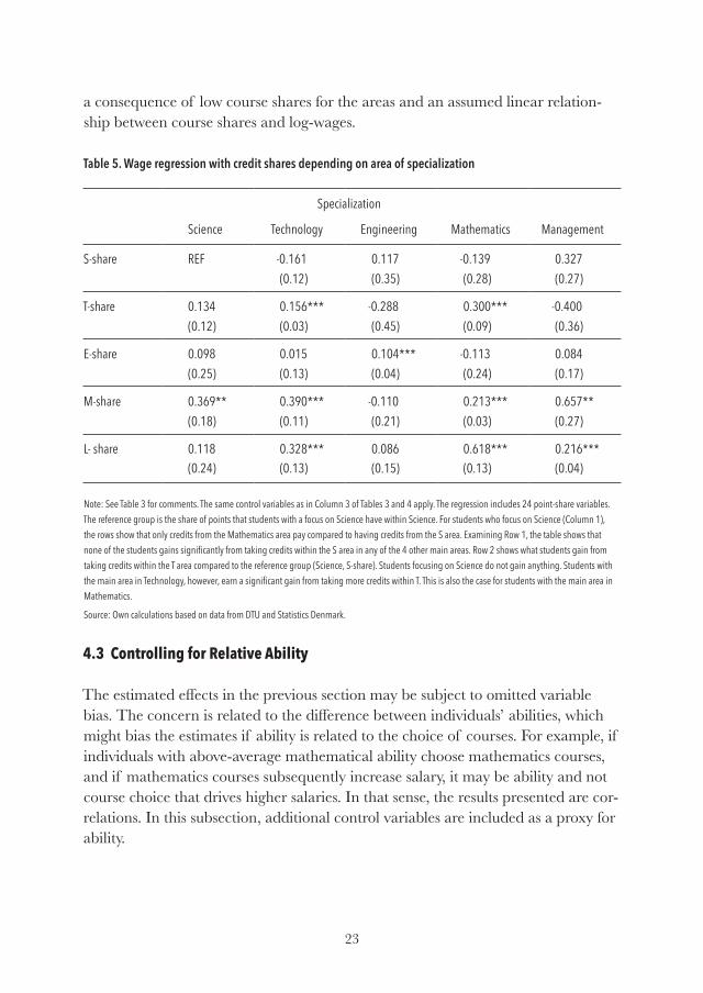
in Table 4. In Table 5, this restriction is relaxed by allowing for salary differences from additional credits within specific areas to vary across the areas of specializa-tion. The coefficients of Table 5 all belong to the same regression and are directly comparable to Table 4, Column 3. All coefficients are compared to the reference group (Science, S-share), where the first element refers to the area of specialization and the second element refers to the share of ECTS credits in Science . It is thereby assumed that the reference group consists of individuals who have full specializa-tion in Science, i .e ., have taken all ECTS credits in science .

Column 1 shows the coefficients of individuals specializing in S . It is seen that gains from taking credits within T, E, M and L are all positive; however, only the point estimate to credits in M is significantly different from zero. The magnitude of this point estimate implies that an individual specialized in S who takes 10 percent of his credits in M earns on average 3.69 percent (=0.369 x 0.1) more compared to specializing fully in S .

Columns 2-5 show the coefficients of individuals specializing in T, E, M and L, respectively. It is seen that all coefficients in the diagonal of the matrix are posi-tive and significantly different from zero. The coefficient for Technology (T-share) equals 0 .156, implying that full specialization in T results in a starting salary 15 .6 percent higher than full specialization in Science . In a similar manner, individuals fully specialized in E have a starting wage that is 10 .4 percent higher than full spe-cialization in S, individuals fully specialized in M have a starting wage that is 21 .3 percent higher, and full specialization in L has a 21 .6 percent higher starting wage .

In addition, two important findings are evident in Table 5 from inspection of the results presented in the rows. First, the M-share enters positively and significantly in four out of five areas of specialization. The only exception is specialization in E . A high M-share implies higher wages, which – to a great extent – are independent of the area of specialization . Coursework in M can, therefore, be interpreted as a gen-eral-purpose skill. This finding is consistent with the finding in Arcidiacono (2004) in an analysis of returns on majors . A similar result is found for management, to some extent . Second, S, T, and E are not correlated significantly off the diagonal, which implies that courses taken within these areas are not positively correlated with wag-es unless they are within the area of specialization . This suggests that S, T, and E can be interpreted as specific-purpose skills .

A final comment on Table 5 is that point estimates for some areas are very high, e.g., the point estimate for M under L-specialization equals 0 .657 . We consider this to be

23

a consequence of low course shares for the areas and an assumed linear relation-ship between course shares and log-wages .

Table 5. Wage regression with credit shares depending on area of specialization

Specialization

Science Technology Engineering Mathematics Management

S-share REF -0.161 0.117 -0.139 0.327(0.12) (0.35) (0.28) (0.27)

T-share 0.134 0.156*** -0.288 0.300*** -0.400(0.12) (0.03) (0.45) (0.09) (0.36)

E-share 0.098 0.015 0.104*** -0.113 0.084(0.25) (0.13) (0.04) (0.24) (0.17)

M-share 0.369** 0.390*** -0.110 0.213*** 0.657**(0.18) (0.11) (0.21) (0.03) (0.27)

L- share 0.118 0.328*** 0.086 0.618*** 0.216***(0.24) (0.13) (0.15) (0.13) (0.04)

Note: See Table 3 for comments. The same control variables as in Column 3 of Tables 3 and 4 apply. The regression includes 24 point-share variables. The reference group is the share of points that students with a focus on Science have within Science. For students who focus on Science (Column 1), the rows show that only credits from the Mathematics area pay compared to having credits from the S area. Examining Row 1, the table shows that none of the students gains significantly from taking credits within the S area in any of the 4 other main areas. Row 2 shows what students gain from taking credits within the T area compared to the reference group (Science, S-share). Students focusing on Science do not gain anything. Students with the main area in Technology, however, earn a significant gain from taking more credits within T. This is also the case for students with the main area in Mathematics.


4.3 Controlling for Relative Ability

The estimated effects in the previous section may be subject to omitted variable bias. The concern is related to the difference between individuals’ abilities, which might bias the estimates if ability is related to the choice of courses. For example, if individuals with above-average mathematical ability choose mathematics courses, and if mathematics courses subsequently increase salary, it may be ability and not course choice that drives higher salaries . In that sense, the results presented are cor-relations . In this subsection, additional control variables are included as a proxy for ability .

2524

Table 6 includes proxies for ability, which consist of pre-tertiary educational choices and the initial choice of a compulsory program at DTU as explanatory variables . The reason is that individuals reveal their relative abilities in previous educational choices . In high school in Denmark, students choose the level and combination of courses in mathematics, physics and chemistry. For example, individuals may choose mathematics and physics at the highest level if they have abilities for that combination . Alternatively, if they have higher ability within chemistry relative to physics, they may well choose chemistry at a higher level than physics . Table 6 con-trols for the combination of courses in mathematics, physics and chemistry .

Table 6. Wage regression with point shares and extra control variables


1 2 3 4

T-share 0.161*** 0.139*** 0.151*** 0.138***(0.03) (0.03) (0.03) (0.03)

E-share 0.049 0.038 0.032 0.026(0.03) (0.04) (0.03) (0.04)

M-share 0.247*** 0.159*** 0.222*** 0.141***(0.03) (0.03) (0.03) (0.04)

L-share 0.152*** 0.128*** 0.133*** 0.116***(0.04) (0.04) (0.04) (0.04)

Grade point average 0.014*** 0.014** 0.013* 0.013**(0.01) (0.01) (0.01) (0.01)

Compulsory course program YES YES

High school information YES YES

N 3525 3525 3287 3287

R-squared 0.057 0.060 0.056 0.058

Note: OLS log-wage regression with robust standard errors in brackets. The compulsory course program is described by 4 dummies, taking the value 1 depending on whether one’s compulsory program was in the S, T, E, or M area. Course level in high school is described by the level combination for Mathematics, Physics and Chemistry. *** p <0.01, ** p <0.05, * p <0.1.


25

Column 1 reproduces the basic regression from Table 4, Column 3 . Column 2 includes the course level for mathematics, physics and chemistry from high school . The estimates obtained on the credit shares are unchanged . Column 3 includes an alternative approximation for relative ability: the choice of courses from the first year of study . Column 4 combines both sets of controls . The qualitative results for the point shares are relatively robust to the additional control variables . However, the point estimate of M decreases from approximately 0 .25 to 0 .14, suggesting that this area is more affected by ability selection.11

In the appendix, additional controls are included for a subsample . This table in-cludes choices broader than the three main mathematical subjects . The results pre-sented in the appendix are similar to those in Table 6 .

4.4 Controlling for Industry Composition of Jobs

Finally, we include industry dummies in the wage regressions. If industry dummies are included to capture wage differentials across industries, two extreme outcomes are possible. The first extreme outcome is that the difference in point estimates disappears completely, i.e., wage differentials are fully explained by wage differ-ences between industries . This outcome would indicate that the course choice is a matter of obtaining the skills required for specific industries. The other extreme outcome is that the point estimates do not change at all when industry dummies are included . This outcome suggests that the composition of courses is not related to industry-specific skills. Both extremes seem unlikely, and an outcome in between is expected . A similar argument can be made for occupations .

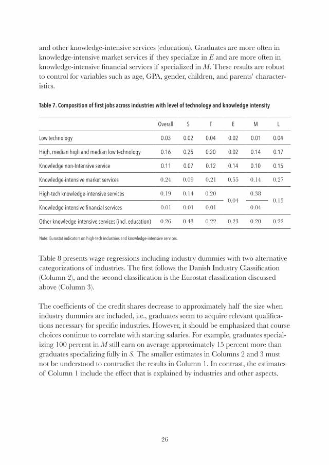
Using Eurostat indicators on high-tech industries and knowledge-intensive servic-es, it is found that most engineering graduates in the sample are occupied in high knowledge-intensive firms.12 However, graduates specialized in management are slightly overrepresented in low technology manufacturing and knowledge non-in-tensive services compared to graduates with other specializations . Moreover, spe-cialization in science is overrepresented in high-technology manufacturing firms

11 We have run an IV regression using average credit shares within specialization area, excluding the individual’s own shares in the graduation year as instruments for the individual’s credit shares . This instrument is inspired by Rose and Betts (2004). The IV estimation coefficients are expected to be different from OLS if high-ability individuals generally choose different combinations of courses. We do not present the results here because the point estimates are similar to those in Table 4 . This is consistent with results not being driven by unobserved variations in ability . 12 http://ec .europa .eu/eurostat/cache/metadata/Annexes/htec_esms_an3 .pdf

2726

and other knowledge-intensive services (education) . Graduates are more often in knowledge-intensive market services if they specialize in E and are more often in knowledge-intensive financial services if specialized in M . These results are robust to control for variables such as age, GPA, gender, children, and parents’ character-istics .

Table 7. Composition of first jobs across industries with level of technology and knowledge intensity

Overall S T E M L

Low technology 0.03 0.02 0.04 0.02 0.01 0.04

High, median high and median low technology 0.16 0.25 0.20 0.02 0.14 0.17

Knowledge non-Intensive service 0.11 0.07 0.12 0.14 0.10 0.15

Knowledge-intensive market services 0 .24 0 .09 0 .21 0 .55 0 .14 0 .27

High-tech knowledge-intensive services 0 .19 0 .14 0 .200 .04

0 .380 .15

Knowledge-intensive financial services 0 .01 0 .01 0 .01 0 .04

Other knowledge-intensive services (incl. education) 0 .26 0 .43 0 .22 0 .23 0 .20 0 .22

Note: Eurostat indicators on high-tech industries and knowledge-intensive services.

Table 8 presents wage regressions including industry dummies with two alternative categorizations of industries. The first follows the Danish Industry Classification (Column 2), and the second classification is the Eurostat classification discussed above (Column 3) .

The coefficients of the credit shares decrease to approximately half the size when industry dummies are included, i.e., graduates seem to acquire relevant qualifica-tions necessary for specific industries. However, it should be emphasized that course choices continue to correlate with starting salaries. For example, graduates special-izing 100 percent in M still earn on average approximately 15 percent more than graduates specializing fully in S . The smaller estimates in Columns 2 and 3 must not be understood to contradict the results in Column 1 . In contrast, the estimates of Column 1 include the effect that is explained by industries and other aspects.

27

Table 8. Wage regression with credit shares and industry dummies


1 2 3

T-share 0.161*** 0.085*** 0.094***(0.03) (0.03) (0.03)

E-share 0.049 0.008 -0.012(0.03) (0.04) (0.04)

M-share 0.247*** 0.156*** 0.181***(0.03) (0.03) (0.03)

L-share 0.152*** 0.074* 0.068*(0.04) (0.04) (0.04)

Grade point average 0.014** 0.022*** 0.021***(0.01) (0.01) (0.01)

Industry dummies NO YES YES

N 3525 3525 3525

R-squared 0.057 0.120 0.112

Note: OLS log-wage regression with robust standard errors in brackets. Danish industry classification is used in Column 2, and Eurostat classification is used in Column 3. *** p <0.01, ** p <0.05, * p <0.1.


2928

5 Conclusion

This article uses a unique dataset from a specific master’s program for engineer-ing graduates to infer the importance of course choices on starting salaries. For simplicity, courses are divided into five areas: Science, Technology, Engineering, Mathematics and Management . The primary conclusion is that course choice is of statistical and economic importance for starting salaries, even when controlling for parental and personal characteristics, including proxies for ability . It is found that it is important to include curriculum choices when comparing educational outcomes, as this adds important explanatory information .

We find large differences across areas of specialization within STEM. Compared to graduates specialized in Science (S), graduates specialized in Mathematics (M) have a starting wage that is 20 percent higher, graduates specialized in Technology (T) have a starting wage that is approximately 15 percent higher, and graduates specialized in Engineering (E) have a starting wage of a similar magnitude . More-over, large variations in wages exist within the four STEM areas, which can partly be explained by course choice. Specifically, courses in M are associated with higher wages in most areas of specialization, which indicates that M is a general-purpose skill. This result echoes Arcidiacono (2004), which finds similar results for a study of university education types . Contrary to this, S, T and E are to a higher extent specific-purpose skills, as courses in these fields are not associated with higher wages if completed outside the area of specialization .

A limitation of the study is that the estimated effects are not necessarily causal. It cannot be ruled out that the relationships are driven by individual ability, poten-tially leading to biased estimates . We do include observable proxies for ability, such as high school GPA and course choice in high school, to control for ability; the established results are robust against the inclusion of these proxies for ability . How-ever, we may not have controlled sufficiently for ability, and in this sense, the results presented are correlations and not causations. In future research, we will try to find more and better instruments to establish causal results .

29

6 References

Arcidiacono, P. (2004), “Ability sorting and the returns to college major”, Journal of Econometrics, 121 (1-2), 343-37 .

Altonji J., E. Blom & C. Meghi, (2012), “Heterogeneity in human capital invest-ments: High school cirriculum, college major and careers”, Annual Review of Econom-ics 4, 185-223 .

Athey, S., L. F. Katz, A. B. Krueger, S. Levitt and J. Poterba (2007), “What Does Performance in Graduate School Predict? Graduate Economics Education and Student Outcomes”, The American Economic Review, 97 (2), 512-518 .

Bertrand, M., C. Goldin & L. F. Katz (2010), “Dynamics of the Gender Gap for Young Professionals in the Financial and Corporate Sectors”, American Economic Journal: Applied Economics, 2, 228–255.

Bloom, N., & J. Van Reenen (2010), “Why do management practices differ across firms and countries?” The Journal of Economic Perspectives, 203-224 .

Blundell, R., L.L. Dearden, A. Goodman & H. Reed (2000), “The Returns to Higher Education in Britain: Evidence from a British Cohort”, Economic Journal, 110, 82-89 .

Carnevale, A., B. Cheah & A. Hanson (2015), “The Economic Value of College Majors” Washington: Center on Education and the Workforce. https://cew.george-town .edu/cew-reports/valueofcollegemajors/ .

Dalgaard, C-J. L., A. Sørensen & E. Schultz (2009), “Do Human Arts Really Offer a Lower Return to Education?” Copenhagen: Centre for Economic and Business Research .

Dahl, C.M., M. Skibsted & A. Sørensen (2016), “Choice of Electives and Future Leadership - Evidence from Business School Students”, CBS mimeo

Hamermesh, D., & S. Donald (2008), “The effect of college curriculum on earn-ings: An affinity identifier for non-ignorable non-response bias” Journal of Economet-ricsI, 144, 479-491

3130

Iversen, J., N. Malchow-Møller & A. Sørensen (2016), “Success in entrepreneur-ship: a complementarity between schooling and wage-work experience, Small Busi-ness Economics, 47, 437-460

Kahn, L, (2010), “The long-term labor market consequences of graduating from college in a bad economy” Labour Economics, 17, 303–316

Kirkeboen, L., E. Leuven & M. Mogstad (2016), “Field of Study, Earnings, and Self-selection” The Quarterly Journal of Economics, 131(3), 1057-1112

Lazear, E. P. (2012), “Leadership: A personnel economics approach”, Labour Eco-nomics, 19, 92–101

Oreopoulos, P., T. von Wachter, & A. Heisz (2012), “The Short- and Long-Term Career Effects of Graduating in a Recession”, American Economic Journal: Applied Eco-nomics, 4(1): 1–29

Romer, P. M. (1990). “Endogenous Technical Change.” Journal of Political Economy 98(5), 71–102.

Romer, P. M. (2001). “Should the Government Subsidize Supply or Demand in the Market for Scientists and Engineers?”, in: Innovation Policy and the Economy, Vol-ume 1, pages 221-252 National Bureau of Economic Research

Rose, H. & J. Betts (2004). ”The Effect of High School Courses on Earnings” The Review of Economics and Statistics, 96(2), 497-513 .

31

7 Appendix

The following table shows that the results reported in section 4 .1 are robust to a broader set of course combinations . The sample size is reduced to less than half, as data on course level in high school is only available from the school year 1997/1998 and onwards in academic-track high schools in Denmark .

Column 2 re-estimates the results in section 4 .2 for the high school subsample; the coefficients are very persistent. In Column 3, additional high school course level combinations are included . The results are robust to these additional combinations .

Appendix Table 1. Wage regression with point shares and high school control variables (subsample)


1 2 3

T-share 0.151*** 0.137*** 0.135***(0.03) (0.04) (0.03)

E-share 0.032 0.066 0.057(0.03) (0.04) (0.04)

M-share 0.222*** 0.196*** 0.195***(0.03) (0.04) (0.04)

L-share 0.133*** 0.154*** 0.151***(0.04) (0.05) (0.05)

Grade average 0.013* 0.004 0.001(0.01) (0.01) (0.01)

Level combination (Math, Physics, Chemistry) (Math, Physics, Chemistry)(Math, Physics, Chemistry, Biology, English, Second

language)

Sample Full High School High School

N 3287 1609 1609

R-squared 0.056 0.102 0.092

Note: OLS log-wage regression with robust standard errors in brackets. The full sample estimation corresponds to Table 6, Column 3. Column 2 re-estimates the regression in Column 1 for the subsample who went to a Danish academic-track high school. Column 3 adds extra course level combinations. *** p <0.01, ** p <0.05, * p <0.1.


ISSN 0908-3979

The ROCKWOOL Foundation Research Unit

Soelvgade 10, 2 .tv .

DK-1307 Copenhagen K

University Press of Southern Denmark

curriculum choice, educational performance, and …

Documents