Curve Building and Swap Pricing in the

Presence of Collateral and Basis Spreads

S I M O N G U N N A R S S O N

Master of Science Thesis Stockholm, Sweden 2013

Curve Building and Swap Pricing in the Presence of Collateral and Basis

Spreads

S I M O N G U N N A R S S O N

Master’s Thesis in Mathematical Statistics (30 ECTS credits) Master Programme in Mathematics (120 credits) Supervisor at KTH was Boualem Djehiche Examiner was Boualem Djehiche

TRITA-MAT-E 2013:19 ISRN-KTH/MAT/E--13/19--SE Royal Institute of Technology School of Engineering Sciences KTH SCI SE-100 44 Stockholm, Sweden URL: www.kth.se/sci

Abstract

The eruption of the financial crisis in 2008 caused immense widening of both domestic

and cross currency basis spreads. Also, as a majority of all fixed income contracts are now

collateralized the funding cost of a financial institution may deviate substantially from

the domestic Libor. In this thesis, a framework for pricing of collateralized interest rate

derivatives that accounts for the existence of non-negligible basis spreads is implemented.

It is found that losses corresponding to several percent of the outstanding notional may

arise as a consequence of not adapting to the new market conditions.

Keywords: Curve building, swap, basis spread, cross currency, collateral

Acknowledgements

I wish to thank my supervisor Boualem Djehiche as well as Per Hjortsberg and Jacob

Niburg for introducing me to the subject and for providing helpful feedback along the way.

I also wish to express gratitude towards my family who has supported me throughout my

education. Finally, I am grateful that Marcus Josefsson managed to devote a few hours

to proofread this thesis.

Contents

1 Introduction 1

1.1 The Libor-OIS and TED Spreads . . . . . . . . . . . . . . . . . . . . . . . 2

1.2 Tenor Basis Spreads . . . . . . . . . . . . . . . . . . . . . . . . . . . . . . 4

1.3 Cross Currency Basis Spreads . . . . . . . . . . . . . . . . . . . . . . . . . 5

1.4 Previous Research . . . . . . . . . . . . . . . . . . . . . . . . . . . . . . . . 6

1.5 FRA and Swap Pricing Before the Financial Crisis . . . . . . . . . . . . . . 7

2 Theoretical Background 10

2.1 Curve Construction without Collateral . . . . . . . . . . . . . . . . . . . . 10

2.1.1 A Single IRS Market . . . . . . . . . . . . . . . . . . . . . . . . . . 10

2.1.2 An IRS and TS Market . . . . . . . . . . . . . . . . . . . . . . . . . 11

2.1.3 Introducing the Constant Notional CCS . . . . . . . . . . . . . . . 11

2.2 Curve Construction with Collateral . . . . . . . . . . . . . . . . . . . . . . 13

2.2.1 Pricing of Collateralized Derivatives . . . . . . . . . . . . . . . . . . 13

2.2.2 Introducing the OIS . . . . . . . . . . . . . . . . . . . . . . . . . . 14

2.2.3 Curve Construction in a Single Currency . . . . . . . . . . . . . . . 15

2.2.4 Curve Construction in Multiple Currencies . . . . . . . . . . . . . . 15

3 Implementation 18

3.1 Building the USD Curves . . . . . . . . . . . . . . . . . . . . . . . . . . . . 18

3.1.1 The USD Discounting Curve . . . . . . . . . . . . . . . . . . . . . . 18

3.1.2 The USD 3m Forward Curve . . . . . . . . . . . . . . . . . . . . . . 19

3.1.3 The USD 1m Forward Curve . . . . . . . . . . . . . . . . . . . . . . 20

3.1.4 The USD 6m Forward Curve . . . . . . . . . . . . . . . . . . . . . . 22

3.2 Building the EUR Curves . . . . . . . . . . . . . . . . . . . . . . . . . . . 23

3.2.1 The EUR Discounting Curve . . . . . . . . . . . . . . . . . . . . . . 23

3.2.2 The EUR 6m Forward Curve . . . . . . . . . . . . . . . . . . . . . 23

3.2.3 The EUR 1m Forward Curve . . . . . . . . . . . . . . . . . . . . . 24

3.2.4 The EUR 3m Forward Curve . . . . . . . . . . . . . . . . . . . . . 25

3.2.5 The EUR 1y Forward Curve . . . . . . . . . . . . . . . . . . . . . . 25

3.2.6 The Case of USD Collateral . . . . . . . . . . . . . . . . . . . . . . 26

4 Results 27

4.1 The Case of USD . . . . . . . . . . . . . . . . . . . . . . . . . . . . . . . . 27

4.2 The Case of EUR . . . . . . . . . . . . . . . . . . . . . . . . . . . . . . . . 31

4.3 Comparing the Currencies . . . . . . . . . . . . . . . . . . . . . . . . . . . 35

5 Conclusions 36

5.1 Critique . . . . . . . . . . . . . . . . . . . . . . . . . . . . . . . . . . . . . 36

5.2 Suggestions for Further Research . . . . . . . . . . . . . . . . . . . . . . . 37

References 38

Appendices 41

A The Forward Measure 41

B Mark-to-Market Cross Currency Swaps 42

C Day Count Conventions 44

D Swap Conventions 45

E Cubic Spline Interpolation 46

F Proof of Proposition 2.1 48

G Tables 50

G.1 Tables of USD Data . . . . . . . . . . . . . . . . . . . . . . . . . . . . . . 50

G.2 Tables of EUR Data . . . . . . . . . . . . . . . . . . . . . . . . . . . . . . 52

1 Introduction

The global financial meltdown during 2008 inevitably caused a lot of change on the finan-

cial markets. Companies were faced with increased credit and liquidity problems and for

banks this situation affected their trading abilities. Henceforth it became vital to account

for credit and liquidity premia when pricing financial products. The effects were particu-

larly apparent in the market for interest rate products, i.e. FRAs, swaps, swaptions etc.,

and as a consequence professionals started developing new pricing frameworks that would

correctly account for the increased credit and liquidity premia. More specifically, ba-

sis spreads between different tenors and currencies that were negligible (typically smaller

than the bid/ask spread) before the crisis were now much wider. A new pricing framework

would have to account for the magnitudes of these spreads and produce consistent prices

that are arbitrage-free. In practice this entails that one should estimate one forward curve

for each tenor, instead of using one universal forward curve for all tenors. Also, as most

over-the-counter interest rate products are nowadays collateralized the question of how

to correctly discount future cash flows must be raised.

In light of this, the purpose of this thesis is to implement a pricing framework that

accounts for non-negligible basis spreads between tenors and currencies that is also able

to price collateralized products in a desirable manner. The approach will be empirical,

i.e. forward rates and discount factors will be extracted from available market quotes and

we will not develop and implement a framework that models the term structures of basis

spreads.

We will assume basic knowledge of stochastic calculus as covered in Øksendal (2003)

[22]. Martingale pricing of financial derivatives is also assumed a prerequisite and an

introduction is given in Bjork (2009) [3]. Geman et. al. (1995) [12] provides an extensive

discussion on the important technique of changing the numeraire. Also, Friedman (1983)

[8] rigorously presents various essential concepts of analysis, such as fundamental measure

theory and Radon-Nikodym derivatives.

The rest of this paper is structured as follows. The remainder of this chapter provides

a summary of the various spreads that widened during the financial crisis and concludes

with an introduction to swap pricing in the absence of basis spreads. Chapter 2 presents

a framework that accounts for the prevailing basis spreads between tenors and currencies,

with and without the presence of collateral. This framework is later implemented in

Chapter 3, where technical details are covered to a greater extent. Results are discussed

in Chapter 4 and Chapter 5 concludes.

1

1.1 The Libor-OIS and TED Spreads

The USD London Interbank Offered Rate (Libor from now on) is an average of the rates

at which banks think they can obtain unsecured funding. It is managed by the British

Bankers’ Association (BBA) to which the participating banks1 submit their estimated

funding costs. The European equivalent to the Libor is the European Interbank Offered

Rate (Euribor), which is managed by the European Banking Federation. While the Libor

is an average of the perceived funding costs of the participating banks, the Euribor is

an average of the rates at which banks believe a prime bank can get unsecured funding.

Both rates are quoted for a range of tenors, where the 3m and 6m are the most widely

monitored.

An overnight indexed swap is a contract between two parties in which one party pays

a fixed rate (the OIS rate) against receiving the geometric average of the (compound)

overnight rate over the term of the contract. In the US, the overnight rate is the effective

Federal Funds rate whereas in Europe it is the Euro Overnight Index Average (Eonia)

rate.2 The OIS rate can now be viewed upon as a measure of the market’s expectation on

the overnight rate until maturity (Thornton, 2009) [29]. Because no principal is exchanged

and since funds typically are exchanged only at maturity there is very little default risk

inherent in the OIS market.

Due to the low risk of default associated with the OIS rate the spread between the

Libor and the OIS rate should give an indication of the default risk in the interbank

market. In fact, the Libor-OIS spread is considered a much wider measure of the health

of the banking system, for example Morini (2009) [21] emphasizes that liquidity risk3 also

is explanatory for the Libor-OIS spread. Cui et. al. (2012) [6] moreover suggests that

increased overall market volatility and industry-specific problems may cause the Libor-

OIS spread to widen. A general flight to safety whereby banks are reluctant to tie-up

liquidity over longer periods of time may also cause the spread to increase, as mentioned

in the Swedish Riksbank’s survey of the Swedish financial markets (2012) [28]. Recently,

Filipovic and Trolle (2012) [7] suggested an approach of decomposing the Libor-OIS spread

into default and non-default components.

Figure 1.1 depicts the Libor-OIS and Euribor-OIS spreads for 3m rates. As mentioned

in Sengupta (2008) [27], the Libor-OIS spread spiked at 365 basis points on October 10th

2008, presumably due to the broad ”illiquidity wave” that followed the bankruptcy of

1A list of the banks contributing to the Libor fixing is found at http://www.bbalibor.com/panels/usd.2The effective Federal Funds rate is computed as a transaction-weighted average of the rates on overnight

unsecured loans that banks make between each other. The banks in question do not entirely coincide

with the Libor panel, which is the case for the Eonia rate.3Liquidity risk is defined as the risk that banks cannot convert their assets into cash.

2

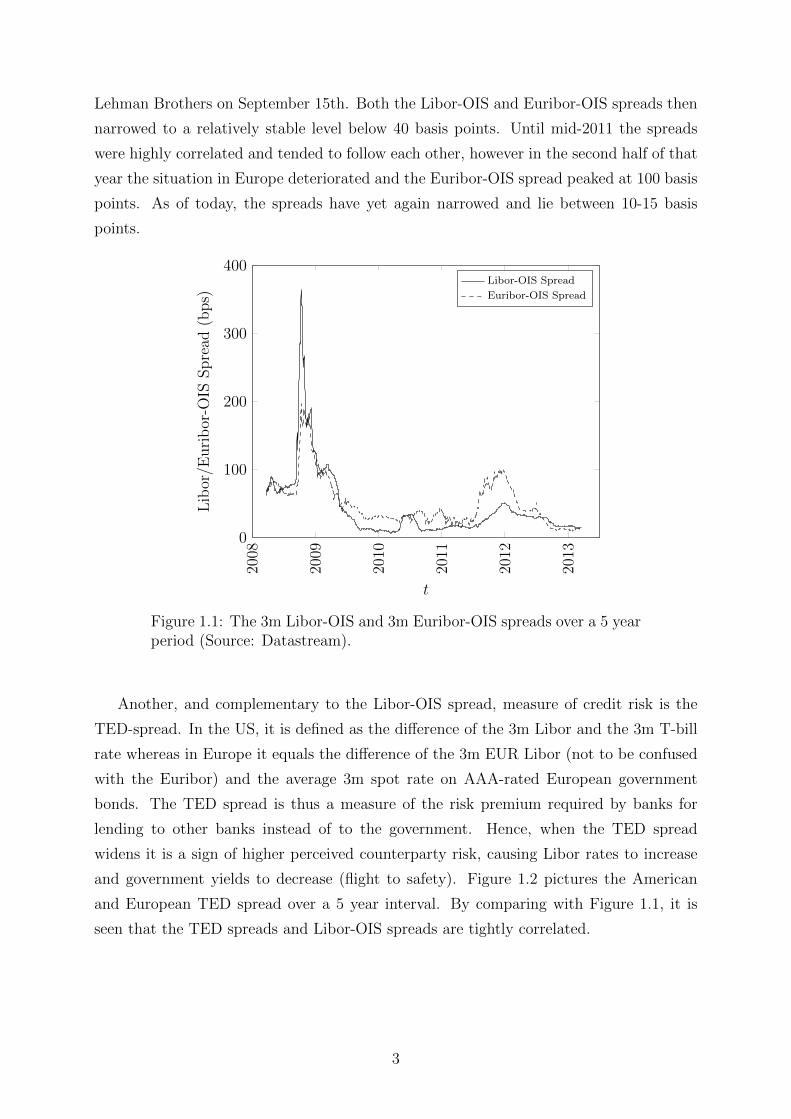
Lehman Brothers on September 15th. Both the Libor-OIS and Euribor-OIS spreads then

narrowed to a relatively stable level below 40 basis points. Until mid-2011 the spreads

were highly correlated and tended to follow each other, however in the second half of that

year the situation in Europe deteriorated and the Euribor-OIS spread peaked at 100 basis

points. As of today, the spreads have yet again narrowed and lie between 10-15 basis

points.

2008

2009

2010

2011

2012

2013

0

100

200

300

400

t

Lib

or/E

uri

bor

-OIS

Spre

ad(b

ps)

Libor-OIS Spread

Euribor-OIS Spread

Figure 1.1: The 3m Libor-OIS and 3m Euribor-OIS spreads over a 5 yearperiod (Source: Datastream).

Another, and complementary to the Libor-OIS spread, measure of credit risk is the

TED-spread. In the US, it is defined as the difference of the 3m Libor and the 3m T-bill

rate whereas in Europe it equals the difference of the 3m EUR Libor (not to be confused

with the Euribor) and the average 3m spot rate on AAA-rated European government

bonds. The TED spread is thus a measure of the risk premium required by banks for

lending to other banks instead of to the government. Hence, when the TED spread

widens it is a sign of higher perceived counterparty risk, causing Libor rates to increase

and government yields to decrease (flight to safety). Figure 1.2 pictures the American

and European TED spread over a 5 year interval. By comparing with Figure 1.1, it is

seen that the TED spreads and Libor-OIS spreads are tightly correlated.

3

2008

2009

2010

2011

2012

2013

0

50

100

150

200

250

300

350

t

TE

DSpre

ad(b

ps)

USD TED Spread

EUR TED Spread

Figure 1.2: The American and European TED spreads over a 5 yearperiod (Source: Datastream).

1.2 Tenor Basis Spreads

A tenor basis swap is a floating for floating swap where the payments are linked to indices

of different tenors. The payments may for example be 6m Libor semiannually on the

first leg and 3m Libor quarterly on the other. Tuckman and Porfirio (2003) [30] shows

that in a default-free environment, a tenor basis swap should trade flat. This means that

lenders are indifferent between receiving the 6m rate semiannually or the 3m rate rolled

over every quarter, and the same goes for other tenors. In reality, the Libor rates have

built in credit premia and it is an accepted fact that these premia differ between tenors.

For example, lending at 6m Libor is associated with more counterparty risk than rolling

lending at 3m Libor. In order to clear markets, the 6m Libor must thus be set higher than

the rate implied by the 3m Libor in order to compensate for the higher counterparty risk.

However, in a tenor basis swap counterparty risk can be eliminated with collateralization

and the advantage of receiving 6m Libor is mitigated by a spread added to the leg paying

3m Libor. Hence, in the presence of credit risk tenor basis swaps do not trade flat, but

with a spread added to the leg with the shorter tenor.

Morini (2009) [21] suggests some explanations as to why lending at a longer tenor is

associated with more counterparty risk as compared to rolling lending at a shorter tenor.

Firstly, in case of default in the 3m-6m period, the 6m lender loses all his interest whereas

the 3m roller receives interest for the first 3 months. Even though both lenders lose the

4

notional, the 3m roller is better off. Also, if the credit conditions of the counterparty

worsen during the first 3 months the 3m roller can exit at par and move on to another

counterparty. The 6m lender instead has to unwind the position at a cost that incorporates

the increased risk of default. Compared to the 3m roller that exits at par, the 6m lender

is worse off. However, in the opposite situation, i.e. that the credit conditions for the

counterparty improve, the 6m lender may be better off than the 3m roller. This suggests

that there is no overall gain for the 3m roller, but since there are commercial reasons

for not unwinding a contract when it is convenient for the lender, the 3m roller has an

advantage.

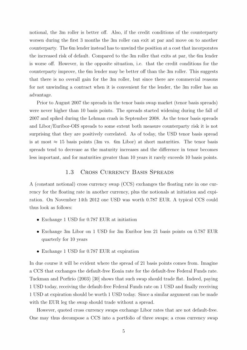
Prior to August 2007 the spreads in the tenor basis swap market (tenor basis spreads)

were never higher than 10 basis points. The spreads started widening during the fall of

2007 and spiked during the Lehman crash in September 2008. As the tenor basis spreads

and Libor/Euribor-OIS spreads to some extent both measure counterparty risk it is not

surprising that they are positively correlated. As of today, the USD tenor basis spread

is at most ≈ 15 basis points (3m vs. 6m Libor) at short maturities. The tenor basis

spreads tend to decrease as the maturity increases and the difference in tenor becomes

less important, and for maturities greater than 10 years it rarely exceeds 10 basis points.

1.3 Cross Currency Basis Spreads

A (constant notional) cross currency swap (CCS) exchanges the floating rate in one cur-

rency for the floating rate in another currency, plus the notionals at initiation and expi-

ration. On November 14th 2012 one USD was worth 0.787 EUR. A typical CCS could

thus look as follows:

• Exchange 1 USD for 0.787 EUR at initiation

• Exchange 3m Libor on 1 USD for 3m Euribor less 21 basis points on 0.787 EUR

quarterly for 10 years

• Exchange 1 USD for 0.787 EUR at expiration

In due course it will be evident where the spread of 21 basis points comes from. Imagine

a CCS that exchanges the default-free Eonia rate for the default-free Federal Funds rate.

Tuckman and Porfirio (2003) [30] shows that such swap should trade flat. Indeed, paying

1 USD today, receiving the default-free Federal Funds rate on 1 USD and finally receiving

1 USD at expiration should be worth 1 USD today. Since a similar argument can be made

with the EUR leg the swap should trade without a spread.

However, quoted cross currency swaps exchange Libor rates that are not default-free.

One may thus decompose a CCS into a portfolio of three swaps; a cross currency swap

5

that exchanges the default-free Eonia rate for the default-free Federal Funds rate, a USD

tenor basis swap that exchanges the Federal Funds rate for the 3m Libor and a EUR tenor

basis swap that exchanges the Eonia for the 3m Euribor. It is now apparent that the cross

currency basis spread derives from the difference between local tenor basis spreads. Now

assume that the 3m Euribor has more credit risk than the 3m Libor. In a collateralized

swap without default risk a stream of 3m Euribor would then be worth more than a

stream of 3m Libor. To compensate for this advantage a negative spread is added to the

leg paying EUR.

The situation above is exactly what prevails on the markets. Figure 1.3 shows how the

3m USDEUR cross currency basis spread has been negative during the last three years.

It is clearly seen that the spread reached −150 basis points in the latter half of 2011,

presumably caused by the then worsening situation in the Euro area. As the markets

calmed the spread narrowed and it is now less than −30 basis points for all maturities.

2010

2011

2012

2013

−160

−140

−120

−100

−80

−60

−40

−20

0

t

USD

EU

RC

ross

Curr

ency

Bas

isSpre

ad(b

ps)

USDEUR Spread

Figure 1.3: The 3m USDEUR cross currency basis spread over a 3 yearperiod (Source: Datastream).

1.4 Previous Research

The works of Hull (2011) [17] and Ron (2000) [26] cover how to price interest rate swaps

in a market absent of basis spreads. The focus lies on bootstrapping a single yield curve

that is used both for discounting and extracting forward rates. This approach is briefly

6

covered in Section 1.5. Once equipped with a discrete set of yields, various interpolation

techniques for obtaining a continuous yield curve are discussed in Hagan and West (2006)

[13] and Hagan and West (2008) [14]. To avoid arbitrage, the interpolation scheme needs

to produce positive forward rates. It is also desired that the obtained forward rates are

stable and that the interpolation function only changes nearby if an input is changed (i.e.

it is local).

Henrard (2007) [15] takes one step towards refining the conventional pricing framework

by addressing the effects from changing the discounting curve. In Henrard (2010) [16], he

further proposes a valuation framework where one forward curve is built for each Libor

tenor. Similar work is done in Ametrano and Bianchetti (2009) [1], where a scheme that

is able to recover the market swap rates is developed. However, as multiple discount rates

exist within the same currency, their model is subject to arbitrage. The arbitrage-free

model proposed in Bianchetti (2008) [2] is in one sense an improvement, but as noted in

Fujii et. al. (2009a) [9] curve calibration cannot be separated from option calibration,

which makes the model somewhat impractical. Mercurio (2009) [20] introduces a new

Libor market model that is based on modeling the joint evolution of implied forward

rates and FRA rates, where the log-normal case with and without stochastic volatility

is analyzed. Johannes and Sundaresan (2009) [19] and Whittall (2010a) [32] further

develop the multi-curve pricing framework by considering the impact of collateralization

on swap rates, whereas Whittall (2010b) [31] discusses which discount rate to use in an

uncollateralized agreement. Other works on the same topic include Morini (2009) [21]

and Chibane et. al. (2009) [5].

Fujii et. al. (2010) [11] presents a method that consistently treats interest rate swaps,

tenor basis swaps, overnight indexed swaps and cross currency basis swaps, where the

effects from collateralization are explicitly addressed. This framework is refined in Fujii

et. al. (2009a) [9], where a model of dynamic basis spreads is introduced. Finally,

Filipovic and Trolle (2012) [7] proposes a term structure of interbank risk that is derived

from observed basis spreads. Moreover, the term structure is decomposed into default

(credit) and non-default components. It is shown that default risk increases with maturity

whereas the non-default component is more dominant in the short term.

1.5 FRA and Swap Pricing Before the Financial Crisis

The forward Libor rate contracted at time t for [Tn−1, Tn] is defined by

L(t, Tn−1, Tn) =1

δn−1,n

(Z(t, Tn−1)

Z(t, Tn)− 1

),

7

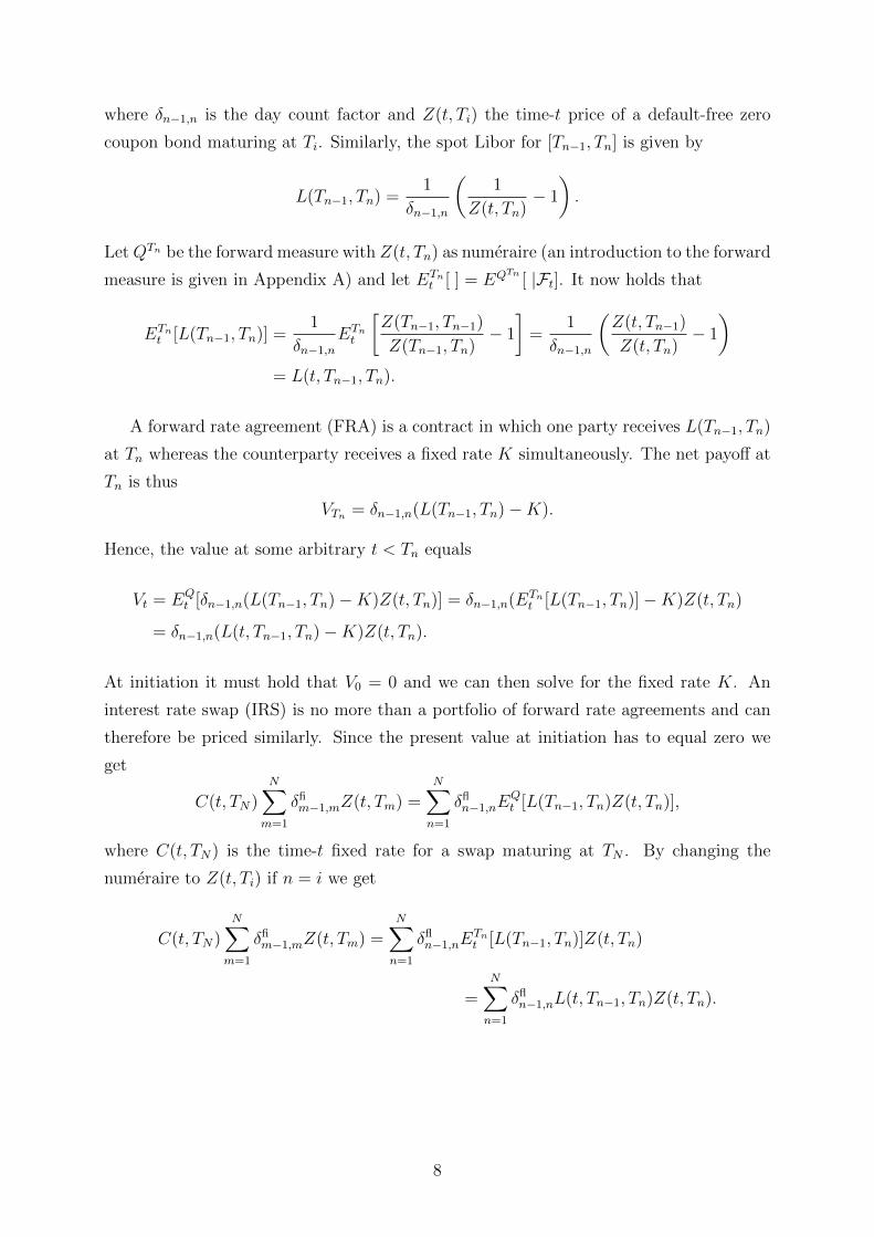
where δn−1,n is the day count factor and Z(t, Ti) the time-t price of a default-free zero

coupon bond maturing at Ti. Similarly, the spot Libor for [Tn−1, Tn] is given by

L(Tn−1, Tn) =1

δn−1,n

(1

Z(t, Tn)− 1

).

LetQTn be the forward measure with Z(t, Tn) as numeraire (an introduction to the forward

measure is given in Appendix A) and let ETnt [ ] = EQTn

[ |Ft]. It now holds that

ETnt [L(Tn−1, Tn)] =

1

δn−1,n

ETnt

[Z(Tn−1, Tn−1)

Z(Tn−1, Tn)− 1

]=

1

δn−1,n

(Z(t, Tn−1)

Z(t, Tn)− 1

)= L(t, Tn−1, Tn).

A forward rate agreement (FRA) is a contract in which one party receives L(Tn−1, Tn)

at Tn whereas the counterparty receives a fixed rate K simultaneously. The net payoff at

Tn is thus

VTn = δn−1,n(L(Tn−1, Tn)−K).

Hence, the value at some arbitrary t < Tn equals

Vt = EQt [δn−1,n(L(Tn−1, Tn)−K)Z(t, Tn)] = δn−1,n(ETn

t [L(Tn−1, Tn)]−K)Z(t, Tn)

= δn−1,n(L(t, Tn−1, Tn)−K)Z(t, Tn).

At initiation it must hold that V0 = 0 and we can then solve for the fixed rate K. An

interest rate swap (IRS) is no more than a portfolio of forward rate agreements and can

therefore be priced similarly. Since the present value at initiation has to equal zero we

get

C(t, TN)N∑m=1

δfim−1,mZ(t, Tm) =

N∑n=1

δfln−1,nE

Qt [L(Tn−1, Tn)Z(t, Tn)],

where C(t, TN) is the time-t fixed rate for a swap maturing at TN . By changing the

numeraire to Z(t, Ti) if n = i we get

C(t, TN)N∑m=1

δfim−1,mZ(t, Tm) =

N∑n=1

δfln−1,nE

Tnt [L(Tn−1, Tn)]Z(t, Tn)

=N∑n=1

δfln−1,nL(t, Tn−1, Tn)Z(t, Tn).

8

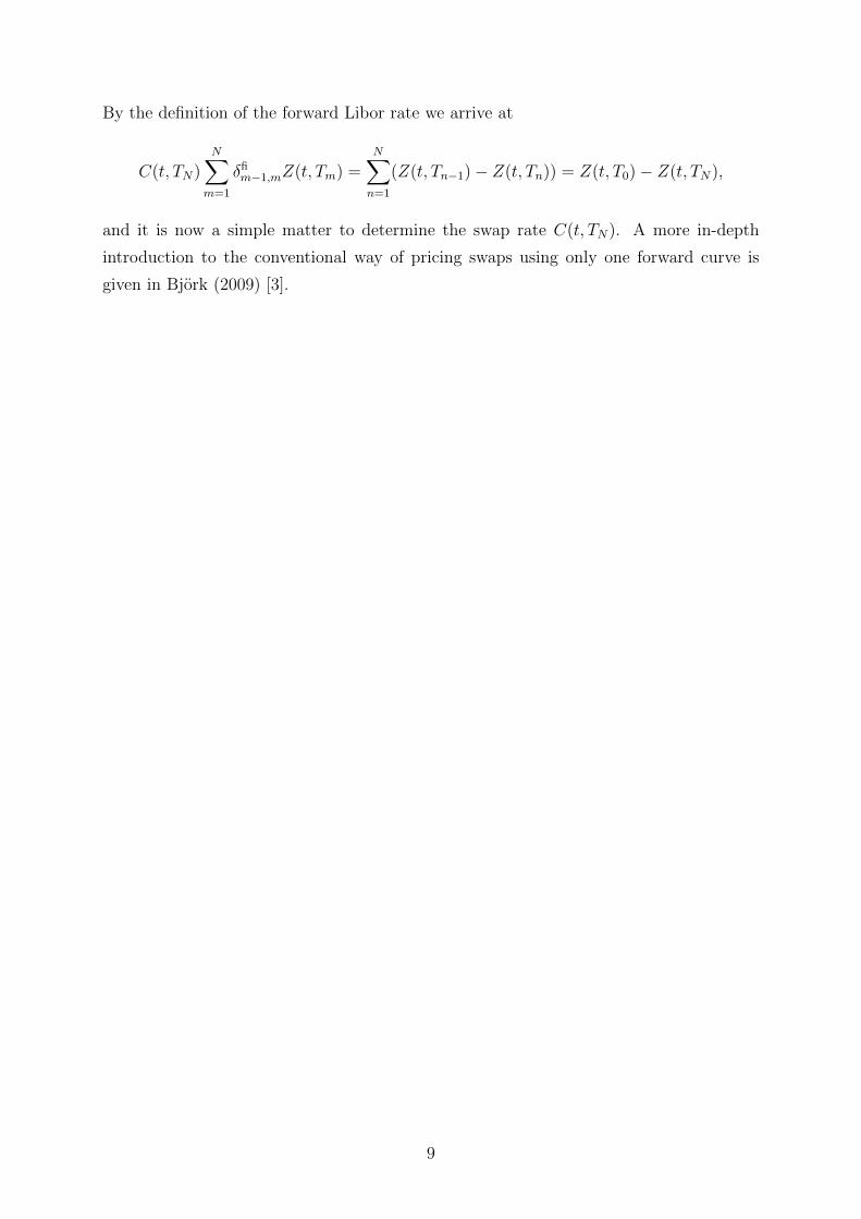
By the definition of the forward Libor rate we arrive at

C(t, TN)N∑m=1

δfim−1,mZ(t, Tm) =

N∑n=1

(Z(t, Tn−1)− Z(t, Tn)) = Z(t, T0)− Z(t, TN),

and it is now a simple matter to determine the swap rate C(t, TN). A more in-depth

introduction to the conventional way of pricing swaps using only one forward curve is

given in Bjork (2009) [3].

9

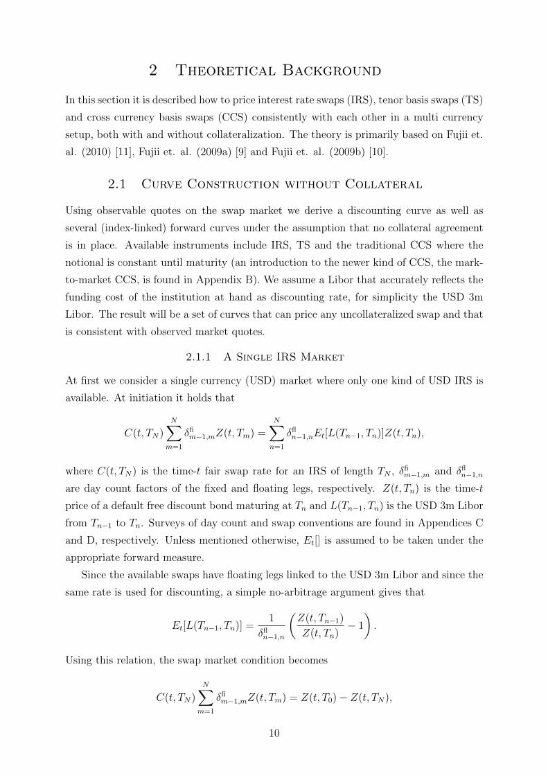
2 Theoretical Background

In this section it is described how to price interest rate swaps (IRS), tenor basis swaps (TS)

and cross currency basis swaps (CCS) consistently with each other in a multi currency

setup, both with and without collateralization. The theory is primarily based on Fujii et.

al. (2010) [11], Fujii et. al. (2009a) [9] and Fujii et. al. (2009b) [10].

2.1 Curve Construction without Collateral

Using observable quotes on the swap market we derive a discounting curve as well as

several (index-linked) forward curves under the assumption that no collateral agreement

is in place. Available instruments include IRS, TS and the traditional CCS where the

notional is constant until maturity (an introduction to the newer kind of CCS, the mark-

to-market CCS, is found in Appendix B). We assume a Libor that accurately reflects the

funding cost of the institution at hand as discounting rate, for simplicity the USD 3m

Libor. The result will be a set of curves that can price any uncollateralized swap and that

is consistent with observed market quotes.

2.1.1 A Single IRS Market

At first we consider a single currency (USD) market where only one kind of USD IRS is

available. At initiation it holds that

C(t, TN)N∑m=1

δfim−1,mZ(t, Tm) =

N∑n=1

δfln−1,nEt[L(Tn−1, Tn)]Z(t, Tn),

where C(t, TN) is the time-t fair swap rate for an IRS of length TN , δfim−1,m and δfl

n−1,n

are day count factors of the fixed and floating legs, respectively. Z(t, Tn) is the time-t

price of a default free discount bond maturing at Tn and L(Tn−1, Tn) is the USD 3m Libor

from Tn−1 to Tn. Surveys of day count and swap conventions are found in Appendices C

and D, respectively. Unless mentioned otherwise, Et[] is assumed to be taken under the

appropriate forward measure.

Since the available swaps have floating legs linked to the USD 3m Libor and since the

same rate is used for discounting, a simple no-arbitrage argument gives that

Et[L(Tn−1, Tn)] =1

δfln−1,n

(Z(t, Tn−1)

Z(t, Tn)− 1

).

Using this relation, the swap market condition becomes

C(t, TN)N∑m=1

δfim−1,mZ(t, Tm) = Z(t, T0)− Z(t, TN),

10

where Z(t, T0) is the discounting factor from time-t to the first fixing date (and can be

determined by the ON-rate). The discounting factors can now be uniquely determined

by sequentially solving

Z(t, Tm) =Z(t, T0)− C(t, Tm)

∑m−1i=1 δfi

i−1,iZ(t, Ti)

1 + C(t, Tm)δfim−1,m

.

This procedure requires that all necessary maturities are in fact traded and the difficulty

that arises when this is not the case is further treated in Section 3. Also, interpolation has

to be carried out in order get a continuous curve of discounting factors and corresponding

forward USD 3m-Libor rates. This topic is further covered in Section 3 and more deeply

in Appendix E.

2.1.2 An IRS and TS Market

We now consider a (still single currency) market where TS as well as IRS with floating legs

linked to USD Libor rates of varying tenor are available. To price an IRS with a floating

leg linked to, for example, the USD 1m Libor, we cannot due to the existence of tenor

basis spreads use the USD 3m Libor forward curve. It is hence necessary to determine a

set of USD 1m Libor forward rates. This can be done by using the quoted USD 1m/3m

TS, where one party pays USD 1m Libor plus a spread monthly and receives USD 3m

Libor quarterly. The resulting conditions become

C(t, TN)N∑m=1

δfim−1,mZ(t, Tm) =

N∑n=1

δ3mn−1,nEt[L

3m(Tn−1, Tn)]Z(t, Tn),

N∑k=1

δ1mk−1,k(Et[L

1m(Tk−1, Tk)] + TS(t, TN))Z(t, Tk) =N∑n=1

δ3mn−1,nEt[L

3m(Tn−1, Tn)]Z(t, Tn),

where TS(t, TN) is the time-t 1m/3m tenor basis spread at maturity TN . The discount

factors and corresponding USD 3m Libor rates are computed as in Section 2.1.1. Through

the basis swaps and proper interpolation it is then possible to compute a continuous set

of USD 1m Libor rates. It is also straightforward to derive forward curves of different

tenors (6m, 1y for example) by adding more TS.

2.1.3 Introducing the Constant Notional CCS

In this section, we expand the model to allow for multiple currencies and for the existence

of a constant notional CCS. More specifically, USD and EUR are the relevant currencies

and the USD 3m Libor is still the discounting rate. Curve construction for US-based

institutions is done as in Sections 2.1.1 and 2.1.2, however for European institutions

one has to account for the cross currency basis spread inherent in the CCS. Thus, the

11

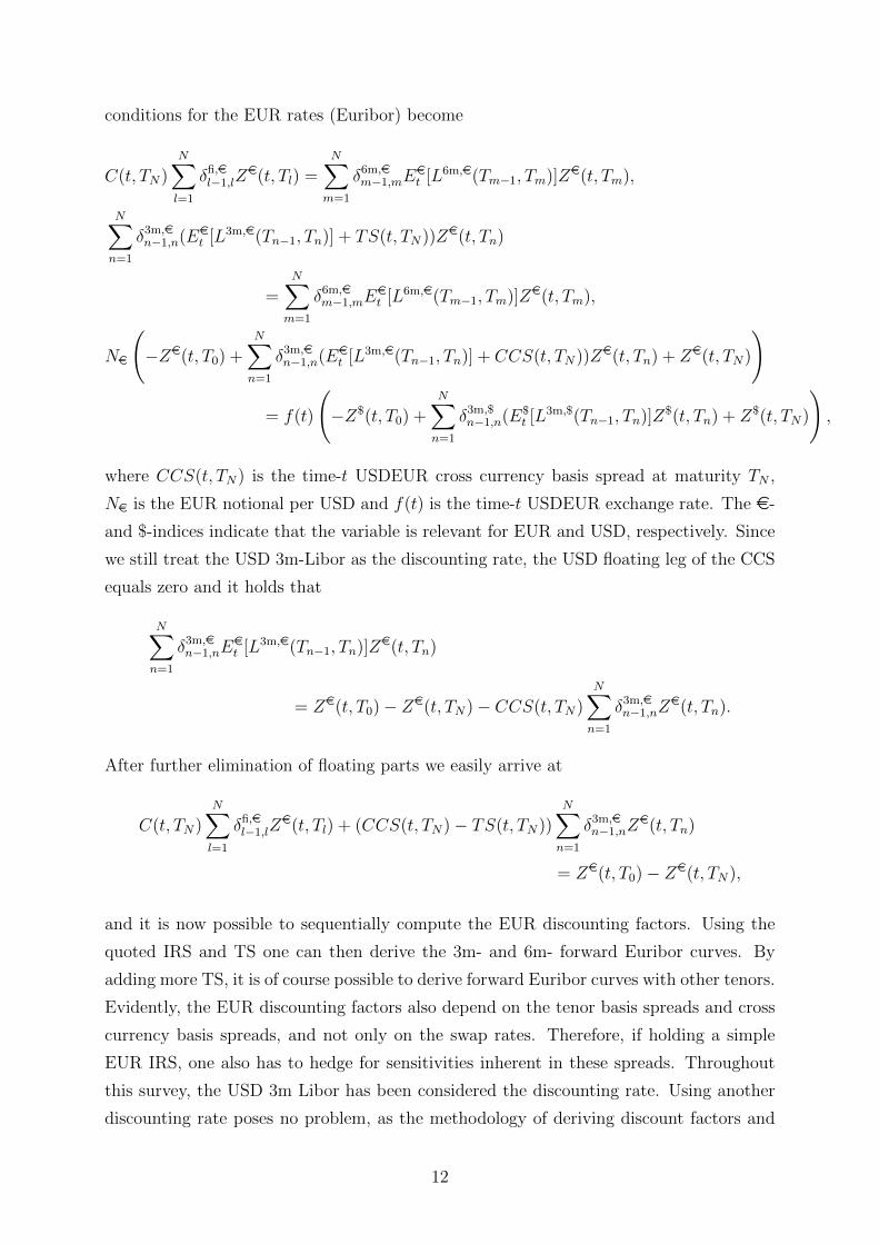
conditions for the EUR rates (Euribor) become

C(t, TN)N∑l=1

δfi,el−1,lZ

e(t, Tl) =N∑m=1

δ6m,em−1,mE

et [L6m,e(Tm−1, Tm)]Ze(t, Tm),

N∑n=1

δ3m,en−1,n(Eet [L3m,e(Tn−1, Tn)] + TS(t, TN))Ze(t, Tn)

=N∑m=1

δ6m,em−1,mE

et [L6m,e(Tm−1, Tm)]Ze(t, Tm),

Ne

(−Ze(t, T0) +

N∑n=1

δ3m,en−1,n(Eet [L3m,e(Tn−1, Tn)] + CCS(t, TN))Ze(t, Tn) + Ze(t, TN)

)

= f(t)

(−Z$(t, T0) +

N∑n=1

δ3m,$n−1,n(E$

t [L3m,$(Tn−1, Tn)]Z$(t, Tn) + Z$(t, TN)

),

where CCS(t, TN) is the time-t USDEUR cross currency basis spread at maturity TN ,

Ne is the EUR notional per USD and f(t) is the time-t USDEUR exchange rate. The e-

and $-indices indicate that the variable is relevant for EUR and USD, respectively. Since

we still treat the USD 3m-Libor as the discounting rate, the USD floating leg of the CCS

equals zero and it holds that

N∑n=1

δ3m,en−1,nE

et [L3m,e(Tn−1, Tn)]Ze(t, Tn)

= Ze(t, T0)− Ze(t, TN)− CCS(t, TN)N∑n=1

δ3m,en−1,nZ

e(t, Tn).

After further elimination of floating parts we easily arrive at

C(t, TN)N∑l=1

δfi,el−1,lZ

e(t, Tl) + (CCS(t, TN)− TS(t, TN))N∑n=1

δ3m,en−1,nZ

e(t, Tn)

= Ze(t, T0)− Ze(t, TN),

and it is now possible to sequentially compute the EUR discounting factors. Using the

quoted IRS and TS one can then derive the 3m- and 6m- forward Euribor curves. By

adding more TS, it is of course possible to derive forward Euribor curves with other tenors.

Evidently, the EUR discounting factors also depend on the tenor basis spreads and cross

currency basis spreads, and not only on the swap rates. Therefore, if holding a simple

EUR IRS, one also has to hedge for sensitivities inherent in these spreads. Throughout

this survey, the USD 3m Libor has been considered the discounting rate. Using another

discounting rate poses no problem, as the methodology of deriving discount factors and

12

forward rates will be analogous to what has been covered herein.

2.2 Curve Construction with Collateral

According to the ISDA Margin Survey [18], close to 80% of all trades with fixed income

derivatives during 2012 were collateralized. For large dealers, this number approaches

90%. As the existence of a collateral agreement substantially reduces the credit risk

inherent in the trade it becomes questionable to apply standard Libor discounting when

pricing a certain product. In this section, it is explained how to price a collateralized

product and more specifically how collateralization affects curve construction for swap

pricing.

2.2.1 Pricing of Collateralized Derivatives

In a collateralized trade, the party whose contract has a positive present value receives

collateral from the counterparty. To compensate for this the party has to pay a certain

margin called ”collateral rate” on the outstanding collateral. In case of cash collateral,

the collateral rate is usually the overnight rate for the collateral currency, i.e. the Federal

Funds rate for USD or the Eonia rate for EUR. To avoid problems with non-linearity,

we assume that mark-to-market and collateral posting is made continuously. Also, the

posted cash collateral is assumed to cover 100% of the contract’s present value. As

collateral posting is commonly done on a daily basis, these simplifications are probably

not too far from reality, at least not for liquid currencies. Since counterparty default risk

can now be neglected, it is possible to recover a linear relationship among payments.

With collateral posted in domestic currency and collateral rate c(s) at time s, the

time-t value h(t) of a derivative h maturing at T is given by the following proposition.

Proposition 2.1.

h(t) = EQt

[e−

∫ Tt c(s)dsh(T )

],

where EQ[] is the expectation with the money-market account as numeraire.

For a proof we refer to Appendix F. If collateral is posted in foreign currency, the

value at time t of the derivative is furthermore given by

h(t) = EQt

[e−

∫ Tt r(s)ds

(e∫ Tt (rf (s)−cf (s))(d)s

)h(T )

],

where r(s) and rf (s) are the domestic and foreign risk-free rates, respectively. cf (s) is

the collateral rate on collateral posted in foreign currency. It can now be seen that in

a collateralized trade future cash flows should be discounted by the collateral rate. As

13

the overnight rate can differ significantly from the Libor, it becomes evident that Libor

discounting is no longer appropriate.

2.2.2 Introducing the OIS

Under the assumption that the collateral rate on cash equals the overnight rate one

can determine collateralized discounted factors by using quoted overnight indexed swaps

(OIS). An OIS exchanges a fixed coupon for a daily compounded overnight rate, where

the dates of the two payments typically coincide. Hence, between two payment dates Tl−1

and Tl the floating leg paysTl∏

s=Tl−1

(1 + δsc(s))− 1

multiplied by the notional. Here, δs is the daily accrual factor and c(s) is the collateral

rate at time s. By approximating daily compounding with continuous compounding, we

getTl∏

s=Tl−1

(1 + δsc(s))− 1 ≈ e∫ TlTl−1

c(s)ds − 1.

If we further assume that the OIS is perfectly collateralized with 100% cash it holds that

(as shown in Section 2.2.1)

S(t, TN)N∑l=1

δfil−1,lE

Qt

[e−

∫ Tlt c(s)ds

]=

N∑l=1

EQt

[e−

∫ Tlt c(s)ds

(e∫ TlTl−1

c(s)ds − 1

)],

where S(t, TN) is the time-t fair swap rate for an OIS of length TN . By denoting the

collateralized discount factors with

D(t, Tl) = EQt

[e−

∫ Tlt c(s)ds

]we arrive at

S(t, TN)N∑l=1

δfil−1,lD(t, Tl) = D(t, T0)−D(t, TN).

It is now a simple matter to sequentially derive the discount factors by

D(t, Tl) =D(t, T0)− S(t, Tl)

∑l−1i=1 δ

fii−1,iD(t, Ti)

1 + S(t, Tl)δfil−1,l

,

and a continuous discount curve is obtained by appropriate splining. Information on

common market conventions for overnight indexed swaps is found in Appendix D.

14

2.2.3 Curve Construction in a Single Currency

In a single currency, the construction of forward Libor curves of different tenors is very

similar to that of Section 2.1.2. After deriving the collateralized discount curve as in

Section 2.2.2, one can compute, let’s say, 1m and 3m Libor forward rates through the

conditions

C(t, TN)N∑m=1

δfim−1,mD(t, Tm) =

N∑n=1

δ3mn−1,nE

ct [L

3m(Tn−1, Tn)]D(t, Tn),

N∑k=1

δ1mk−1,k(E

ct [L

1m(Tk−1, Tk)] + TS(t, TN))D(t, Tk) =N∑n=1

δ3mn−1,nE

ct [L

3m(Tn−1, Tn)]D(t, Tn),

where Ect [] is the expectation with the appropriate D(t, Tn) as numeraire. It is of course

possible to add more TS to derive forward curves with other tenors.

2.2.4 Curve Construction in Multiple Currencies

Unlike the single-currency setup, where collateral and swap payments are in the same

currency, we must now allow for collateral and swap payments to be of different currencies.

As in Section 2.1.3 the constant notional CCS will be used as calibration instrument (how

to use the mark-to-market CCS for curve calibration is covered in Appendix B) and the

relevant currencies will be USD and EUR. Also, the Federal Funds rate will be treated as

the risk-free rate. Since it is also the collateral rate for USD, it now holds that

D$(t, T ) = EQ$

t

[e−

∫ Tt c$(s)ds

]= EQ$

t

[e−

∫ Tt r$(s)ds

]= Z$(t, T ).

Conditions for USD-collateralized USD swaps (with the USD 1m/3m TS) are thus

S$(t, TN)N∑l=1

δfi,$l−1,lZ

$(t, Tl) = Z$(t, T0)− Z$(t, TN),

C$(t, TN)N∑m=1

δfi,$m−1,mZ

$(t, Tm) =N∑n=1

δ3m,$n−1,nE

$t [L

3m,$(Tn−1, Tn)]Z$(t, Tn),

N∑k=1

δ1m,$k−1,k(E

$t [L

1m,$(Tk−1, Tk)] + TS$(t, TN))Z$(t, Tk)

=N∑n=1

δ3m,$n−1,nE

$t [L

3m,$(Tn−1, Tn)]Z$(t, Tn).

15

Similarly, conditions for EUR-collateralized EUR swaps (with the EUR 3m/6m TS) are

Se(t, TN)N∑l=1

δfi,el−1,lD

e(t, Tl) = De(t, T0)−De(t, TN),

Ce(t, TN)N∑l=1

δfi,el−1,lD

e(t, Tl) =N∑m=1

δ6m,em−1,mE

c,et [L6m,e(Tm−1, Tm)]De(t, Tm),

N∑n=1

δ3m,en−1,n(Ec,e

t [L3m,e(Tn−1, Tn)] + TSe(t, TN))De(t, Tn)

=N∑m=1

δ6m,em−1,mE

c,et [L6m,$(Tm−1, Tm)]De(t, Tm).

Of course, more TS conditions can be added if needed.

We now turn our attention to USD-collateralized EUR swaps. Assume the existence

of a USD cash-collateralized USDEUR constant notional CCS. With the results of Section

2.2.1 it holds that4

−Ze(t, T0) +N∑n=1

δ3m,en−1,n(Eet [L3m,e(Tn−1, Tn)] + CCS(t, TN))Ze(t, Tn) + Ze(t, TN)

= N$f(t)

(−Z$(t, T0) +

N∑n=1

δ3m,$n−1,nE

$t [L

3m,$(Tn−1, Tn)]Z$(t, Tn) + Z$(t, TN)

),

where the right-hand side is previously known. It is however not possible to derive both

the EUR zero coupon bond prices and the EUR forward rates through this condition only.

Ideally quotes for USD-collateralized EUR IRS and TS are available, which would allow

us to easily derive the sets of discount factors and forward rates. Alternatively, one could

assume that

Eet [Le(Tn−1, Tn)] = Ec,et [Le(Tn−1, Tn)].

In this approach we thus neglect the change of numeraire, and the approximation is

reasonable if the EUR risk-free and collateral rates have similar dynamic properties. This

4The sum in the LHS is given by

N∑n=1

δ3m,en−1,nE

Qe

t

[e−

∫ Tnt

re(s)ds(e−

∫ Tnt

(r$(s)−c$(s))ds)

(L(Tn−1, Tn) + CCS(t, TN ))]

=

N∑n=1

δ3m,en−1,nE

Qe

t

[e−

∫ Tnt

re(s)ds (L(Tn−1, Tn) + CCS(t, TN ))]

=

N∑n=1

δ3m,en−1,n(Eet [L3m,e(Tn−1, Tn)] + CCS(t, TN ))Ze(t, Tn).

16

enables us to sequentially derive the EUR zero coupon bond prices.

We finally consider the case of EUR-collateralized USD swaps. The conditions for

EUR-collateralized USD IRS and constant notional CCS are

C$(t, TN)N∑m=1

δfi,$m−1,mZ

$(t, Tm)E$t

[e∫ Tmt (re(s)−ce(s))ds

]=

N∑n=1

δ3m,$n−1,nZ

$(t, Tn)E$t

[e∫ Tnt (re(s)−ce(s))dsL3m,$(Tn−1, Tn)

],

N∑n=1

δ3m,$n−1,nZ

$(t, Tn)E$t

[e∫ Tnt (re(s)−ce(s))dsL3m,$(Tn−1, Tn)

]= N$

(−De(t, T0) +

N∑n=1

δ3m,en−1,n(Ec,e

t [L3m,e(Tn−1, Tn)] + CCS(t, TN))De(t, Tn) +De(t, TN)

),

where CCS(t, TN) and C$(t, TN) are the fair rates for the EUR-collateralized CCS and

USD IRS, respectively. With these instruments at hand, it is possible to determine[e∫ Tmt (re(s)−ce(s))ds

]and

[e∫ Tnt (re(s)−ce(s))dsL3m,$(Tn−1, Tn)

]for each m and n. By adding EUR-collateralized USD tenor basis swaps, it is also possible

to derive Libor curves of other tenors.

17

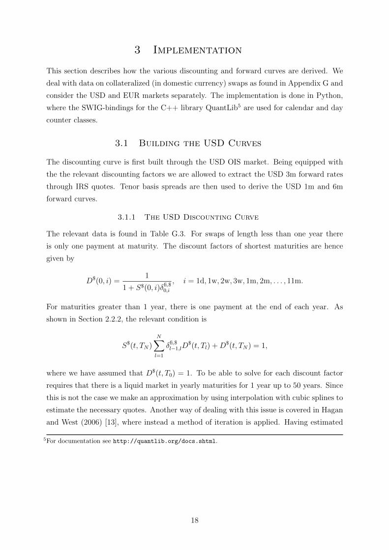
3 Implementation

This section describes how the various discounting and forward curves are derived. We

deal with data on collateralized (in domestic currency) swaps as found in Appendix G and

consider the USD and EUR markets separately. The implementation is done in Python,

where the SWIG-bindings for the C++ library QuantLib5 are used for calendar and day

counter classes.

3.1 Building the USD Curves

The discounting curve is first built through the USD OIS market. Being equipped with

the the relevant discounting factors we are allowed to extract the USD 3m forward rates

through IRS quotes. Tenor basis spreads are then used to derive the USD 1m and 6m

forward curves.

3.1.1 The USD Discounting Curve

The relevant data is found in Table G.3. For swaps of length less than one year there

is only one payment at maturity. The discount factors of shortest maturities are hence

given by

D$(0, i) =1

1 + S$(0, i)δfi,$0,i

, i = 1d, 1w, 2w, 3w, 1m, 2m, . . . , 11m.

For maturities greater than 1 year, there is one payment at the end of each year. As

shown in Section 2.2.2, the relevant condition is

S$(t, TN)N∑l=1

δfi,$l−1,lD

$(t, Tl) +D$(t, TN) = 1,

where we have assumed that D$(t, T0) = 1. To be able to solve for each discount factor

requires that there is a liquid market in yearly maturities for 1 year up to 50 years. Since

this is not the case we make an approximation by using interpolation with cubic splines to

estimate the necessary quotes. Another way of dealing with this issue is covered in Hagan

and West (2006) [13], where instead a method of iteration is applied. Having estimated

5For documentation see http://quantlib.org/docs.shtml.

18

all required OIS rates, we are able to solve the following system of equations:

S$(0, 1y)δfi,$0,1y + 1 0 · · · 0

S$(0, 2y)δfi,$0,1y S$(0, 2y)δfi,$

1y,2y + 1 · · · 0

.... . .

...

.... . . 0

S$(0, 50y)δfi,$0,1y · · · · · · S$(0, 50y)δfi,$

49y,50y + 1

D$(0, 1y)

D$(0, 2y)

...

...

D$(0, 50y)

=

1

1

...

...

1

.

We are now supplied with estimates of yearly discount factors from 1 year up to 50 years.

However, we only use those with maturities corresponding to quoted overnight index

swaps. To obtain a continuous set of discount factors, interpolation with cubic splines is

applied to this subset.

3.1.2 The USD 3m Forward Curve

To build the USD 3m forward curve we use the 3m spot Libor in Table G.1 together with

the IRS quotes in Table G.3. The relevant condition is now

C$(t, TN)N∑m=1

δfi,$m−1,mD

$(t, Tm) =N∑n=1

δ3m,$n−1,nE

c,$t [L3m,$(Tn−1, Tn)]D$(t, Tn),

and is previously known from Section 2.2.4. As we have already built the discounting

curve it is now possible to extract the 3m forward rates. However, just as in Section 3.1.1

we need to interpolate the swap curve to obtain estimates of all necessary swap rates.

Also, since the fixed leg pays semiannually and the floating leg quarterly the resulting

system of equations would become underdetermined. To mitigate this problem we assume

that the forward rates are piecewise flat, i.e. that

Ec,$t [L3m,$(6m, 9m)] = Ec,$

t [L3m,$(9m, 12m)],

Ec,$t [L3m,$(12m, 15m)] = Ec,$

t [L3m,$(15m, 18m)]

19

and so on. Since we already know the 3m spot Libor, the resulting system of equations is

δ3m,$3m,6mD

$(0, 6m) 0 · · · 0

δ3m,$3m,6mD

$(0, 6m)∑12m

i=9m δ3m,$i−3m,iD

$(0, i) · · · 0

......

......

......

... 0

δ3m,$3m,6mD

$(0, 6m)∑12m

i=9m δ3m,$i−3m,iD

$(0, i) · · ·∑600m

i=597m δ3m,$i−3m,iD

$(0, i)

Ec,$t [L3m,$(3m, 6m)]

Ec,$t [L3m,$(9m, 12m)]

...

...

Ec,$t [L3m,$(597m, 600m)]

=

C$(0, 6m)∑6m

n=6m δfi,$n−6m,nD

$(0, n) − δ3m,$0,3mE

c,$t [L3m,$(0, 3m)]D$(0, 3m)

C$(0, 1y)∑12m

n=6m δfi,$n−6m,nD

$(0, n) − δ3m,$0,3mE

c,$t [L3m,$(0, 3m)]D$(0, 3m)

...

...

C$(0, 50y)∑600m

n=6m δfi,$n−6m,nD

$(0, n) − δ3m,$0,3mE

c,$t [L3m,$(0, 3m)]D$(0, 3m)

.

By solving this system we obtain an array of USD 3m forward Libors, however we choose

to discard those with maturities that do not coincide with the maturities of quoted interest

rate swaps. Interpolation with cubic splines on the remainder then gives us the continuous

3m forward curve.

3.1.3 The USD 1m Forward Curve

To construct the USD 1m forward curve we use the 1m spot Libor in Table G.1, the

quoted tenor basis spreads in Table G.2 and the quoted 1m IRS in Table G.3. The 1m

implied swap rate is first computed by

C$(0, 1m) =δ1m,$

0,1m

δfi,$0,1m

Ec,$t [L1m,$(0, 1m)],

and is added to the array of quoted IRS with maturities up to 12 months. We extract the

forward rates with maturities ≤ 12m through the condition

C$(t, TN)N∑k=1

δfi,$k−1,kD

$(t, Tk) =N∑k=1

δ1m,$k−1,kE

c,$t [L1m,$(Tk−1, Tk)]D

$(t, Tk),

20

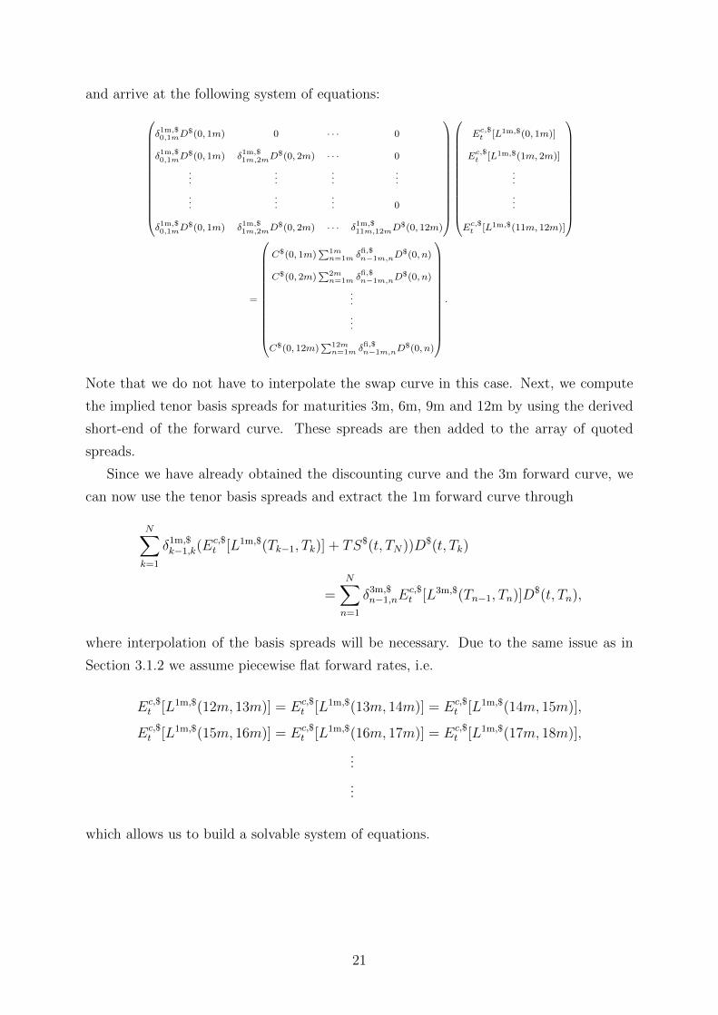
and arrive at the following system of equations:

δ1m,$0,1mD

$(0, 1m) 0 · · · 0

δ1m,$0,1mD

$(0, 1m) δ1m,$1m,2mD

$(0, 2m) · · · 0

......

......

......

... 0

δ1m,$0,1mD

$(0, 1m) δ1m,$1m,2mD

$(0, 2m) · · · δ1m,$11m,12mD

$(0, 12m)

Ec,$t [L1m,$(0, 1m)]

Ec,$t [L1m,$(1m, 2m)]

...

...

Ec,$t [L1m,$(11m, 12m)]

=

C$(0, 1m)∑1m

n=1m δfi,$n−1m,nD

$(0, n)

C$(0, 2m)∑2m

n=1m δfi,$n−1m,nD

$(0, n)

...

...

C$(0, 12m)∑12m

n=1m δfi,$n−1m,nD

$(0, n)

.

Note that we do not have to interpolate the swap curve in this case. Next, we compute

the implied tenor basis spreads for maturities 3m, 6m, 9m and 12m by using the derived

short-end of the forward curve. These spreads are then added to the array of quoted

spreads.

Since we have already obtained the discounting curve and the 3m forward curve, we

can now use the tenor basis spreads and extract the 1m forward curve through

N∑k=1

δ1m,$k−1,k(E

c,$t [L1m,$(Tk−1, Tk)] + TS$(t, TN))D$(t, Tk)

=N∑n=1

δ3m,$n−1,nE

c,$t [L3m,$(Tn−1, Tn)]D$(t, Tn),

where interpolation of the basis spreads will be necessary. Due to the same issue as in

Section 3.1.2 we assume piecewise flat forward rates, i.e.

Ec,$t [L1m,$(12m, 13m)] = Ec,$

t [L1m,$(13m, 14m)] = Ec,$t [L1m,$(14m, 15m)],

Ec,$t [L1m,$(15m, 16m)] = Ec,$

t [L1m,$(16m, 17m)] = Ec,$t [L1m,$(17m, 18m)],

...

...

which allows us to build a solvable system of equations.

21

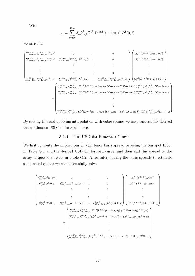
With

A =12m∑i=1m

δ1m,$i−1m,iE

c,$t [L1m,$(i− 1m, i)]D$(0, i)

we arrive at

∑15mi=13m δ1m,$

i−1m,iD$(0, i) 0 · · · 0∑15m

i=13m δ1m,$i−1m,iD

$(0, i)∑18m

i=16m δ1m,$i−1m,iD

$(0, i) · · · 0

......

......

......

... 0∑15mi=13m δ1m,$

i−1m,iD$(0, i)

∑18mi=16m δ1m,$

i−1m,iD$(0, i) · · ·

∑600mi=598m δ1m,$

i−1m,iD$(0, i)

Ec,$t [L1m,$(14m, 15m)]

Ec,$t [L1m,$(17m, 18m)]

...

...

Ec,$t [L1m,$(599m, 600m)]

=

∑15mn=3m δ3m,$

n−3m,nEc,$t [L3m,$(n− 3m,n)]D$(0, n) − TS$(0, 15m)

∑15mi=1m δ1m,$

i−1m,iD$(0, i) −A∑18m

n=3m δ3m,$n−3m,nE

c,$t [L3m,$(n− 3m,n)]D$(0, n) − TS$(0, 18m)

∑18mi=1m δ1m,$

i−1m,iD$(0, i) −A

...

...∑600mn=3m δ3m,$

n−3m,nEc,$t [L3m,$(n− 3m,n)]D$(0, n) − TS$(0, 600m)

∑600mi=1m δ1m,$

i−1m,iD$(0, i) −A

.

By solving this and applying interpolation with cubic splines we have successfully derived

the continuous USD 1m forward curve.

3.1.4 The USD 6m Forward Curve

We first compute the implied 6m 3m/6m tenor basis spread by using the 6m spot Libor

in Table G.1 and the derived USD 3m forward curve, and then add this spread to the

array of quoted spreads in Table G.2. After interpolating the basis spreads to estimate

semiannual quotes we can successfully solve

δ6m,$0,6mD

$(0, 6m) 0 · · · 0

δ6m,$0,6mD

$(0, 6) δ6m,$6m,12mD

$(0, 12m) · · · 0

......

......

......

... 0

δ6m,$0,6mD

$(0, 6) δ6m,$6m,12mD

$(0, 12m) · · · δ6m,$594m,600mD

$(0, 600m)

Ec,$t [L6m,$(0, 6m)]

Ec,$t [L6m,$(6m, 12m)]

...

...

Ec,$t [L6m,$(594m, 600m)]

=

∑6mn=3m δ3m,$

n−3m,n(Ec,$t [L3m,$(n− 3m,n)] + TS$(0, 6m))D$(0, n)∑12m

n=3m δ3m,$n−3m,n(Ec,$

t [L3m,$(n− 3m,n)] + TS$(0, 12m))D$(0, n)

...

...∑600mn=3m δ3m,$

n−3m,n(Ec,$t [L3m,$(n− 3m,n)] + TS$(0, 600m))D$(0, n)

.

22

Next, we filter out the forward rates with maturities that correspond to maturities of

quoted instruments. After performing interpolation (again with cubic splines) on this

subset we have successfully completed the construction of the USD 6m forward curve.

3.2 Building the EUR Curves

In this section it is described how the EUR discounting curve is constructed through

the OIS market, how EUR 1m, 3m, 6m and 1y forward curves are built using quoted

interest rate and tenor basis swaps and, finally, how to derive the discounting curve for

USD-collateralized EUR swaps.

3.2.1 The EUR Discounting Curve

The construction of the EUR discounting curve is analogous to that of the USD discount-

ing curve. For maturities < 1y we get the discount factors by

De(0, i) =1

1 + Se(0, i)δfi,e0,i

, i = 1d, 1w, 2w, 3w, 1m, 2m, . . . , 11m.

For maturities ≥ 1y the condition

Se(t, TN)N∑l=1

δfi,el−1,lD

e(t, Tl) +De(t, TN) = 1

holds, and we thus end up with the following set of equations:

Se(0, 1y)δfi,e0,1y + 1 0 · · · 0

Se(0, 2y)δfi,e0,1y Se(0, 2y)δfi,e

1y,2y + 1 · · · 0

.... . .

...

.... . . 0

Se(0, 50y)δfi,e0,1y · · · · · · Se(0, 50y)δfi,e

49y,50y + 1

De(0, 1y)

De(0, 2y)

...

...

De(0, 50y)

=

1

1

...

...

1

.

To obtain a continuous set of discount factors we apply the same procedure as in Section

3.1.1. The input data is found in Table G.7.

3.2.2 The EUR 6m Forward Curve

The EUR 6m forward curve is built in a similar manner as the USD 3m forward curve,

only that the interest rate swaps now pay fixed annually and floating semiannually. The

relevant condition is thus

Ce(t, TN)N∑l=1

δfi,el−1,lD

e(t, Tl) =N∑m=1

δ6m,em−1,mE

c,et [L6m,e(Tm−1, Tm)]De(t, Tm),

23

where the input swap rates and 6m Euribor are found in Tables G.7 and G.4, respectively.

Having determined the appropriate discount factors and assuming that (compare with

Section 3.1.2)

Ec,et [L6m,e(12m, 18m)] = Ec,e

t [L3m,e(18m, 24m)],

Ec,et [L6m,e(24m, 30m)] = Ec,e

t [L6m,e(30m, 36m)],

...

...

the 6m forward rates are computed by solving

δ6m,e6m,12mD

e(0, 12m) 0 · · · 0

δ6m,e6m,12mD

e(0, 12m)∑24m

i=18m δ6m,ei−6m,iD

e(0, i) · · · 0

......

......

......

... 0

δ6m,e6m,12mD

e(0, 12m)∑24m

i=18m δ6m,ei−6m,iD

e(0, i) · · ·∑600m

i=594m δ6m,ei−6m,iD

e(0, i)

Ec,et [L6m,e(6m, 12m)]

Ec,et [L6m,e(18m, 24m)]

...

...

Ec,et [L6m,e(594m, 600m)]

=

Ce(0, 1y)∑12m

n=12m δfi,en−12m,nD

e(0, n) − δ6m,e0,6mE

c,et [L6m,e(0, 6m)]De(0, 6m)

Ce(0, 2y)∑24m

n=12m δfi,en−12m,nD

e(0, n) − δ6m,e0,6mE

c,et [L6m,e(0, 6m)]De(0, 6m)

...

...

Ce(0, 50y)∑600m

n=12m δfi,en−12m,nD

e(0, n) − δ6m,e0,6mE

c,et [L6m,e(0, 6m)]De(0, 6m)

.

Appropriate splining (a procedure familiar by now) renders the continuous EUR 6m for-

ward curve.

3.2.3 The EUR 1m Forward Curve

To build the EUR 1m forward curve we use the 1m Euribor spot rate in Table G.4, the

quoted 1m/6m tenor basis spreads in Table G.6 and the quoted 1m interest rate swaps in

Table G.7. The procedure is very similar to that of the USD 1m forward curve in Section

3.1.3, apart from a few differences. This time quoted 1m IRS of maturities up to two years

are available, but since they are not so on a monthly basis interpolation of the swap curve

becomes necessary. With the interpolated 1m swap curve we can bootstrap the short-end

of the forward curve (i.e. with maturities ≤ 2 years). Subsequently, the implied 6m, 1y,

18m and 2y tenor basis spreads are computed with the aid of the bootstrapped 1m forward

curve. By initially assuming that the long-end of the 1m forward curve is piecewise flat in

intervals of 6 months (compare with Section 3.1.3) we can successfully compute forward

rates for maturities > 2 years. As usual, forward rates that correspond to maturities

24

of quoted instruments are filtered out before the continuous EUR 1m forward curve is

obtained through interpolation with cubic splines.

3.2.4 The EUR 3m Forward Curve

The short-end of the EUR 3m forward curve is built using the 3m Euribor in Table G.4

and the Euribor futures in Table G.5. As Euribor contracts are available up to, and

including, MAR20156 we can successfully estimate forward rates with maturities up to

30 months using interpolation. After computing the implied 6m, 1y, 18m, 2y and 30m

tenor basis spreads and adding these to the quoted 3m/6m spreads in Table G.6 we end

up with (after customary interpolation of the basis spreads and assuming piecewise flat

forward rates in intervals of 6 months)

∑36mi=33m δ3m,e

i−3m,iDe(0, i) 0 · · · 0∑36m

i=33m δ3m,ei−3m,iD

e(0, i)∑42m

i=39m δ3m,ei−3m,iD

e(0, i) · · · 0

......

......

......

... 0∑36mi=33m δ3m,e

i−3m,iDe(0, i)

∑42mi=39m δ3m,e

i−3m,iDe(0, i) · · ·

∑600mi=597m δ3m,e

i−3m,iDe(0, i)

Ec,et [L3m,e(33m, 36m)]

Ec,et [L3m,e(39m, 42m)]

...

...

Ec,et [L3m,e(597m, 600m)]

=

∑36mn=6m δ6m,e

n−6m,nEc,et [L6m,e(n− 6m,n)]De(0, n) − TSe(0, 36m)

∑36mi=3m δ3m,e

i−3m,iDe(0, i) −A∑42m

n=6m δ6m,en−6m,nE

c,et [L6m,e(n− 6m,n)]De(0, n) − TSe(0, 42m)

∑42mi=3m δ3m,e

i−3m,iDe(0, i) −A

...

...∑600mn=6m δ6m,e

n−6m,nEc,et [L6m,e(n− 6m,n)]De(0, n) − TSe(0, 600m)

∑600mi=3m δ3m,e

i−3m,iDe(0, i) −A

,

where

A =30m∑i=3m

δ3m,ei−3m,iE

c,et [L3m,e(i− 3m, i)]De(0, i).

Now that both the short- and the long-end are estimated we have finished the construction

of the EUR 3m forward curve.

3.2.5 The EUR 1y Forward Curve

The EUR 1y forward curve is constructed using the 1y Euribor spot rate in Table G.4

and the 6m/1y tenor basis spreads in Table G.6. Apart from all intervals in time being

twice as long, this curve is built in exactly the same way as the USD 6m forward curve.

We therefore refer to Section 3.1.4 for more details.

6This refers to a contract starting on the IMM date in March 2015 and maturing on the IMM date in

June 2015. The IMM (International Monetary Market) dates are the third Wednesday of March, June,

September and December.

25

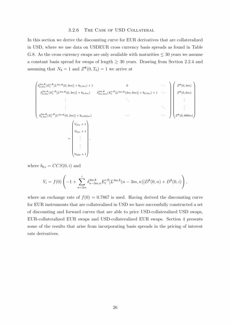
3.2.6 The Case of USD Collateral

In this section we derive the discounting curve for EUR derivatives that are collateralized

in USD, where we use data on USDEUR cross currency basis spreads as found in Table

G.8. As the cross currency swaps are only available with maturities ≤ 30 years we assume

a constant basis spread for swaps of length ≥ 30 years. Drawing from Section 2.2.4 and

assuming that N$ = 1 and Ze(0, T0) = 1 we arrive at

δ3m,e0,3m(Ec,e

t [L3m,e(0, 3m)] + b0,3m) + 1 0 · · ·

δ3m,e0,3m(Ec,e

t [L3m,e(0, 3m)] + b0,6m) δ3m,e3m,6m(Ec,e

t [L3m,e(3m, 6m)] + b0,6m) + 1 · · ·...

. . .

.... . .

δ3m,e0,3m(Ec,e

t [L3m,e(0, 3m)] + b0,600m) · · · · · ·

Ze(0, 3m)

Ze(0, 6m)

...

...

Ze(0, 600m)

=

V3m + 1

V6m + 1

...

...

V600 + 1

,

where b0,i = CCS(0, i) and

Vi = f(0)

(−1 +

i∑n=3m

δ3m,$n−3m,nE

c,$t [L3m,$(n− 3m,n)]D$(0, n) +D$(0, i)

),

where an exchange rate of f(0) = 0.7867 is used. Having derived the discounting curve

for EUR instruments that are collateralized in USD we have successfully constructed a set

of discounting and forward curves that are able to price USD-collateralized USD swaps,

EUR-collateralized EUR swaps and USD-collateralized EUR swaps. Section 4 presents

some of the results that arise from incorporating basis spreads in the pricing of interest

rate derivatives.

26

4 Results

In this section we present the discounting and forward curves as derived in Section 3,

where a discussion on how well these curves are able to replicate the prices of quoted

instruments is included. Moreover, we address the impact basis spreads have on swap

pricing and the importance of correctly adjusting for the existence of such spreads. The

cases of USD and EUR are dealt with separately, where a comparison between the two

currencies concludes the chapter.

4.1 The Case of USD

The discounting and forward curves are shown in Figures 4.1 and 4.2. To be able to

compare the different forward curves we show the implied 6m forward rates for each

tenor. For example, the 6m implied forward rate with basis 1m is computed as

Ect [L

1m(i, i+ 6m)] =

∏6j=1

(1 + δ1m

i+(j−1)m,i+jmEct [L

1m(i+ (j − 1)m, i+ jm)])− 1

δ1mi,i+6m

.

It is seen that the 6m forward curve lies above the 3m forward curve (and the 3m curve

above the 1m curve). This is supposedly due to the higher liquidity and credit risk

associated with lending at 6m Libor as compared to rolling lending at 3m Libor, and is

what one should expect.

With these curves at hand we can price a wide array of USD-collateralized USD swaps,

where the most interesting question is how important it is to adjust for basis spreads when

pricing such swaps. In Figure 4.3 the computed 1m, 3m and 6m swap curves are pictured

along with the market quotes for 3m swaps. The 3m curve seems fairly good at replicating

the quoted swap rates, however as further seen in Table 4.1 there are some discrepancies.

Maturity ∆ (bps)

1y 0.482y 1.123y 1.775y 3.7310y 4.1320y 2.79

Table 4.1: The difference between quoted and estimated USD 3m swaprates (a selection).

That the 3m swap curve on average underestimates the quoted 3m swap rate by 3 basis

points is explained by the assumption we made when constructing the forward curve

27

in Section 3.1.2. As the USD IRS pays floating quarterly but fixed only semiannually

we assumed that the forward curve was piecewise flat in intervals of 6 months. This

assumption was further disregarded when interpolating the bootstrapped forward rates

(since only forward rates that corresponded to maturities of quoted instruments were used

for interpolation) and thus some of the estimated forward rates are lower than implied by

our assumption and the quoted swap rates. Consequently, the value of the floating leg,

and in turn the swap rate, is slightly underestimated. Observe that this would not be

an issue for uncollateralized derivatives, where we could use the relationship between the

discounting factors and forward rates to (almost) perfectly replicate the swap curve.

Figure 4.3 displays how there is a positive spread between the 6m and 3m swap curves

(and similarly for the 3m and 1m curves). This result agrees with theory, since by the

definition of the tenor basis spread we get that

C6m(t, T )− C3m(t, T ) ≈ TS3m,6m(t, T ) > 0,

and so on. The reason for this not being an equality is that day count conventions and/or

payment frequencies might differ between the fixed legs of the interest rate swaps. The

fact that the swap curves do not coincide raises the question of how important it is to

account for basis spreads when pricing interest rate swaps. Assume for example that a

party uses a single (3m forward) curve when pricing derivatives. This party would thus

be willing to pay a higher fixed rate in an IRS with a floating leg linked to the 1m Libor

than what is justified by the basis spreads. This loss can be approximated with

Loss =(C3m(t, T )− C1m(t, T )

)· PV (Discount Factors) ·N ,

where N is the notional and PV (Discount Factors) is the present value of all discount

factors times year fractions. Table 4.2 displays the percentage loss/gain of the notional

that would incur if basis spreads in the USD market are not accounted for properly. For

maturities > 10 years the loss is close to/above 1% for the 1m and 6m swaps, respectively.

This amount is clearly significant and underlines the importance of a pricing framework

that correctly and accurately accounts for basis spreads. That the loss is greater for

6m swaps is in this sense natural, since the 3m/6m basis spreads are greater than the

corresponding 1m/3m spreads.

28

MaturityLoss (%)1m Tenor

Loss (%)6m Tenor

1y 0.09 0.212y 0.19 0.333y 0.28 0.424y 0.38 0.515y 0.49 0.596y 0.58 0.667y 0.65 0.738y 0.71 0.829y 0.76 0.9010y 0.80 0.9812y 0.86 1.1415y 0.91 1.3620y 0.97 1.68

Table 4.2: The loss as a percentage of notional from not accounting forbasis spreads in the USD market.

0 5 10 15 20 25 30 35 40 45 500.3

0.4

0.5

0.6

0.7

0.8

0.9

1

t (years)

D$(0,t

)

USD Discounting Curve

Figure 4.1: The USD discounting curve.

29

0 1 2 3 4 5 6 7 8 9 100

0.5

1

1.5

2

2.5

3

3.5

t (years)

For

war

dR

ate

(%)

1m Forward Curve

3m Forward Curve

6m Forward Curve

Figure 4.2: The USD forward curves.

0 2 4 6 8 10 12 14 16 18 200

0.5

1

1.5

2

2.5

t (years)

Sw

apR

ate

(%)

1m Swap Curve

3m Swap Curve

6m Swap Curve

3m Swap Quotes

Figure 4.3: The USD swap curves along with quotes for 3m USD IRS.

30

4.2 The Case of EUR

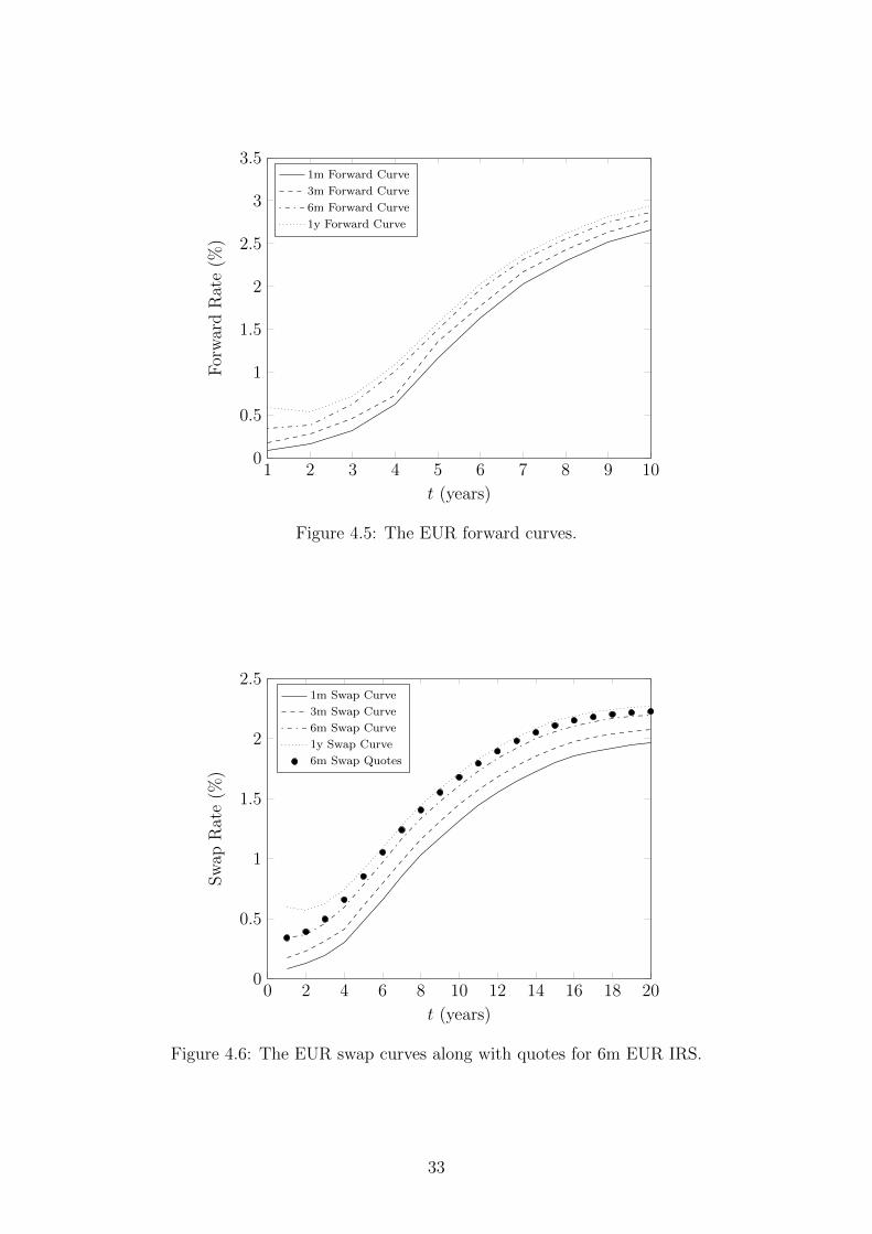
The discounting and forward curves are pictured in Figures 4.4 and 4.5, where the implied

12m forward rates are shown for each tenor. Figure 4.4 also includes the relevant discount

factors for USD-collateralized EUR instruments, where the spread in part is due to the

cross currency basis spreads in Table G.8. As in the case with USD in Section 4.1, the

relative placement of the EUR forward curves agrees well with what is predicted by theory.

The discounting and forward curves are used to construct the EUR-collateralized EUR

swap curves in Figure 4.6, where the quoted 6m swap rates are also displayed. Table 4.3

shows the difference between the quoted rates and the rates computed using the set of

curves. With an average difference of 4.1 basis points it is clear that the pricing framework

Maturity ∆ (bps)

1y -0.272y 2.223y 4.025y 7.2810y 6.7020y 3.25

Table 4.3: The difference between quoted and estimated EUR 6m swaprates (a selection).

underestimates the true swap rate somewhat, where the difference gets smaller as the swap

curve flattens out. The reason for this is the same as in Section 4.1 and was elaborated

further upon there.

Furthermore, Table 4.4 highlights the importance of accounting for basis spreads by

showing the percentage loss (of the notional) that would follow from only using the 6m

forward curve when pricing interest rate swaps, regardless of what tenor the floating leg is

linked to. The loss evidently approaches 4% of the notional for 1m swaps as the maturity

increases. Even for short maturities and independent of tenor, the loss is close to 1%.

For deals with notionals in the ballpark of 10 million EUR or more, the magnitude of the

potential loss is substantial. These numbers thus exemplify how important it could be to

correctly account for basis spreads on a day-to-day basis.

Finally, Figure 4.7 displays the difference in swap rate between USD-collateralized and

EUR-collateralized EUR 6m interest rate swaps. For maturities less than 20 years the

difference is at most around 1 basis point, which obviously is a consequence of the same

curve being used for discounting both the fixed and the floating leg. It is worth remem-

bering that we assumed unchanged forward rates when moving from EUR-collateralized

to USD-collateralized instruments (to derive the relevant discounting curve).

31

MaturityLoss (%)1m Tenor

Loss (%)3m Tenor

Loss (%)1y Tenor

1y 0.26 0.17 0.252y 0.48 0.27 0.413y 0.79 0.44 0.504y 1.18 0.72 0.575y 1.52 0.87 0.656y 1.85 1.06 0.717y 2.13 1.21 0.788y 2.39 1.35 0.849y 2.62 1.46 0.9010y 2.83 1.57 0.9612y 3.18 1.74 1.0715y 3.56 1.90 1.1520y 3.98 2.06 1.24

Table 4.4: The loss as a percentage of notional from not accounting forbasis spreads in the EUR market.

0 5 10 15 20 25 30 35 40 45 50

0.4

0.6

0.8

1

t (years)

De(0,t

)an

dZe(0,t

)

EUR Discounting Curve

EUR Discount Bond Prices

Figure 4.4: The EUR discounting curve together with the EUR zerocoupon bond prices.

32

1 2 3 4 5 6 7 8 9 100

0.5

1

1.5

2

2.5

3

3.5

t (years)

For

war

dR

ate

(%)

1m Forward Curve

3m Forward Curve

6m Forward Curve

1y Forward Curve

Figure 4.5: The EUR forward curves.

0 2 4 6 8 10 12 14 16 18 200

0.5

1

1.5

2

2.5

t (years)

Sw

apR

ate

(%)

1m Swap Curve

3m Swap Curve

6m Swap Curve

1y Swap Curve

6m Swap Quotes

Figure 4.6: The EUR swap curves along with quotes for 6m EUR IRS.

33

0 2 4 6 8 10 12 14 16 18 20−0.2

0

0.2

0.4

0.6

0.8

1

1.2

t (years)

Diff

eren

cein

Sw

apR

ate

(bps)

Figure 4.7: The difference in swap rate between USD-collateralized EUR6m swaps and EUR-collateralized EUR 6m swaps.

34

4.3 Comparing the Currencies

By comparing Tables 4.1 and 4.3 it is seen that both the USD 3m and EUR 6m swap

rates are underestimated by the respective pricing frameworks. With an average difference

between the quoted and estimated swap rate of ≈ 4 bps, the effect is more substantial for

EUR swaps. The effect is even greater when considering the steep part of the swap curve,

where the difference amounts to 7-8 bps for some maturities. For USD swaps, on the other

hand, the quoted swap rate is never underestimated by more than 5 bps. As previously

mentioned, this effect is due to the assumption that forward rates are piecewise flat in

intervals of 6 months (12 months for EUR) in the bootstrapping procedure. In turn, we

made this assumption since the fixed legs pay semiannually and annually for USD and

EUR interest rate swaps, respectively (as compared to quarterly and semiannual floating

payments). To minimize this effect one could instead assume that the dates of the fixed

and floating payments coincide, i.e. that EUR swaps pay fixed semiannually whereas USD

swaps pay fixed quarterly.

Moreover, Tables 4.2 and 4.4 highlight the importance of accounting for basis spreads

in the respective currencies. Whereas the USD loss is at most around 1.7% (20 year 6m

swap), the EUR loss approaches 4% for similar maturities. Obviously, the larger basis

spreads in the EUR market as compared to the USD market are to blame for this. This

is especially true when considering the EUR 1m swaps, where the loss amounts to 2%

even for a swap maturing in 7 years. To incur a loss of similar magnitude in the USD

market, one needs to consider a 6m swap maturing in 26 years from now (for 1m swaps of

maturities less than 50 years, losses of similar magnitude are never possible). Evidently,

it is currently more important to account for basis spreads when pricing European instru-

ments as compared to American. This result is hardly surprising when considering the

withholding state of the European financial climate, where the perceived liquidity/credit

risks remain high.

35

5 Conclusions

To recapitulate, the purpose of this thesis was to implement a pricing framework that

accounts for the basis spreads between different tenors and currencies, with and without

collateralization. Distinct forward curves were built for each available Libor/Euribor

tenor using quoted tenor basis swaps. Furthermore, the quoted overnight indexed swaps

allowed us to build discount curves suitable for pricing collateralized contracts. The cross

currency basis spread between USD and EUR was then used to construct a discount curve

applicable on EUR-denominated instruments that are collateralized with USD cash. The

resulting set of discount and forward curves made it possible to price USD-collateralized

USD instruments as well as USD- and EUR-collateralized EUR instruments.

Section 4 presented the derived discount and forward curves as well as the corre-

sponding swap curves. In particular, two aspects were discussed more deeply. Firstly,

the method of constructing the curves was evaluated by how well it managed to replicate

quoted swap rates. It was seen that the pricing framework underestimates quoted rates

by a few basis points, where the effect was most significant for EUR swaps. Moreover,

we computed the incurred loss from not accounting for basis spreads appropriately. Even

now when basis spreads have narrowed considerably the effect was significant and could

lead to a loss of several percent of the notional, especially for EUR denominated swaps.

Therefore, we can stress the importance for institutions to implement a framework where

basis spreads are not assumed negligible. Mispricing of interest rate products (and of

other asset classes for that matter) could lead to substantial losses, especially if the credit

climate worsens and basis spreads widen.

The rest of this Section is devoted to discussing potential improvements to the curve

construction procedure as well as relevant topics for further research.

5.1 Critique

One drawback is that the derived swap curves underestimate the quoted swap spread by

a few basis points, and the reason for this was explained in Section 4.1. Note that since

not all relevant maturities are available it is not possible to perfectly replicate all swap

rates, however one could try to reach better estimates by for example assuming that the

fixed and floating legs have equal payment frequencies.

Moreover, the interpolation method could be reviewed. We have used interpolation

with cubic splines consistently throughout the curve construction procedure, but as men-

tioned in Hagan and West (2006) [13] this method implicitly treats discrete forward rates

as a property of one of the endpoints of the interval, and not as a property of the entire

interval. It could therefore be an idea to implement interpolation with forward monotone

36

convex splines, as discussed in Hagan and West (2006) [13]. This method also makes sure

that the resulting continuous curve is convex and locally monotone given that the discrete

inputs have the corresponding discrete properties.

Lastly, the quoted cross currency basis swaps are in fact of the mark-to-market type

and do not have constant notionals. One could account for this by adapting the imple-

mentation procedure, but this will not have significant impact on the results.

5.2 Suggestions for Further Research

A natural extension to the empirical approach in this paper is to implement a model with

dynamic basis spreads as proposed in Fujii et. al. (2009) [9] or in Filipovic and Trolle

(2012) [7]. Such model could further be used to price more exotic interest rate derivatives,

for example interest rate swaptions or options on tenor basis swaps.

The implementation procedure could further be extended by computing appropriate

hedging ratios. Of most interest is probably the delta sensitivity of a portfolio consisting

of instruments with a variety of different underlying tenors. Of course, the convexity and

other Greeks could also be of interest.

Finally, the framework implemented in this thesis only produces basis consistent prices

of interest rate products. It is certainly necessary to develop similar frameworks for other

asset classes, for example equity and commodity derivatives.

37

References

[1] Ametrano, F. M., and Bianchetti, M. Bootstrapping the Illiquidity: Multiple

Yield Curves Construction for Market Coherent Forward Rates Estimation. MOD-

ELING INTEREST RATES, Fabio Mercurio, ed., Risk Books, Incisive Media (May

2009).

[2] Bianchetti, M. Two Curves, One Price: Pricing & Hedging Interest Rate Deriva-

tives Decoupling Forwarding and Discounting Yield Curves. Working Paper, Novem-

ber 2008.

[3] Bjork, T. Arbitrage Theory in Continuous Time, vol. 3. Oxford University Press,

2009.

[4] Burden, R. L., and Faires, J. D. Numerical Analysis, vol. 9. Brooks Cole, 2010.

[5] Chibane, M., Selvaraj, J., and Sheldon, G. Building Curves on a Good Basis.

Working Paper, April 2009.

[6] Cui, J., In, F. H., and Maharaj, E. A. What Drives the Libor-OIS Spread?

Evidence from Five Major Currency Libor-OIS Spreads. Working paper, November

2012.

[7] Filipovic, D., and Trolle, A. B. The Term Structure of Interbank Risk. Swiss

Finance Institute Research Paper No. 11-34, October 2012.

[8] Friedman, A. Foundations of Modern Analysis. Dover Publications Inc., 1983.

[9] Fujii, M., Shimada, Y., and Takahashi, A. A Market Model of Interest Rates

with Dynamic Basis Spreads in the Presence of Collateral and Multiple Currencies.

Working paper, 2009.

[10] Fujii, M., Shimada, Y., and Takahashi, A. A Survey on Modeling and Analysis

of Basis Spreads. Working paper, 2009.

[11] Fujii, M., Shimada, Y., and Takahashi, A. A Note on Construction of Multiple

Swap Curves with and without Collateral. CARF Working Paper Series No. CARF-

F-154, 2010.

[12] Geman, H., Karoui, N. E., and Rochet, J. Changes of Numeraire, Changes of

Probability Measure and Option Pricing. Journal of Applied Probability 32(2) (June

1995), 443–458.

38

[13] Hagan, P. S., and West, G. Interpolation Methods for Curve Construction.

Applied Mathematical Finance 13(2) (2006), 89–129.

[14] Hagan, P. S., and West, G. Methods for Constructing a Yield Curve.

WILMOTT Magazine (May 2008), 70–81.

[15] Henrard, M. The Irony in the Derivatives Discounting. Working Paper, March

2007.

[16] Henrard, M. The Irony in the Derivatives Discounting Part II: The Crisis. Working

Paper, December 2009.

[17] Hull, J. Options, Futures and Other Derivatives, vol. 8. Pearson Education, 2011.

[18] International Swaps and Derivatives Association. ISDA Margin Survey

2012, May 2012.

[19] Johannes, M., and Sundaresan, S. The Impact of Collateralization on Swap

Rates. The Journal of Finance 62(1) (February 2007), 383–410.

[20] Mercurio, F. Interest Rates and the Credit Crunch: New Formulas and Market

Models. Bloomberg Portfolio Research Paper No. 2010-01-FRONTIERS (July 2009).

[21] Morini, M. Solving the Puzzle in the Interest Rate Market. Working Paper, October

2009.

[22] Øksendal, B. Stochastic Differential Equations: An Introduction with Applications,

vol. 6. Springer, 2003.

[23] OpenGamma Quantitative Research. Interest Rate Instruments and Market

Conventions Guide, April 2012.

[24] Piterbarg, V. Funding beyond discounting: collateral agreements and derivatives

pricing. Risk Magazine (February 2010), 97–102.

[25] Piterbarg, V. Cooking with collateral. Risk Magazine (August 2012), 58–63.

[26] Ron, U. A Practical Guide to Swap Curve Construction. Bank of Canada, 2000.

[27] Sengupta, R., and Tam, Y. M. The LIBOR-OIS Spread as a Summary Indicator.

Tech. Rep. 25, Federal Reserve Bank of St. Louis Economic Synopses, 2008.

[28] Sveriges Riksbank. Den svenska finansmarknaden, 2012.

39

[29] Thornton, D. L. What the Libor-OIS Spread Says. Tech. Rep. 24, Federal Reserve

Bank of St. Louis Economic Synopses, 2009.

[30] Tuckman, B., and Porfirio, P. Interest Rate Parity, Money Market Basis

Swaps, and Cross-Currency Basis Swaps. Fixed Income Liquid Markets Research,

Lehman Brothers, June 2003.

[31] Whittall, C. Dealing with Funding on Uncollateralised Swaps. Risk Magazine

(June 2010).

[32] Whittall, C. The Price is Wrong. Risk Magazine (March 2010).

40

A The Forward Measure

We begin with a definition of the forward measure.

Definition A.1. The Tn-forward measure QTn is defined as the martingale measure

for the numeraire process Z(t, Tn) = e−∫ Tnt r(s)ds, where r(s) is the short rate process.

This measure should not be confused with the conventional martingale measure Q with

the money market account B = e∫ t0 r(s)ds as numeraire. It can however be shown that the

Radon-Nikodym derivative dQTn

dQis given by

dQTn

dQ=

Z(t, Tn)

B(t)Z(0, T ),

and if assuming that the zero coupon bond dynamics under Q are Wiener driven it holds

that the Girsanov kernel for the transition from Q to QTn equals the bond volatility

σ(t, Tn). The following theorem is now rather evident.

Theorem A.1. The relation Q = QTn holds if and only if r is deterministic.

Finally, let XTn be the value of an arbitrary claim at Tn. Now,XTn

Z(T,T )= XTn is a martingale

under QTn and we arrive at

Theorem A.2. For any claim XTn it holds that

Xt = Z(t, Tn)ETn [XTn|Ft],

where ETn [ ] denotes expectation under QTn.

Bear in mind that Z(t, Tn) can be observed directly on the market at time t (or boot-

strapped from other quoted instruments).

41

B Mark-to-Market Cross Currency Swaps

The mark-to-market cross currency swap and the constant notional cross currency swap

are different in one aspect. In the mark-to-market cross currency swap the notional on

the leg paying Libor flat (i.e. the USD leg) is adjusted at all Libor fixing times, where

the calculation is based on the prevailing spot exchange rate. The difference between the

old and the new notional amount is then paid or received. Conceptually, the USD leg can

be seen as a portfolio of one period constant notional cross currency swaps, where the

terminal and initial exchanges correspond to the transfer of notional.

We first consider a USD-collateralized USDEUR mark-to-market cross currency swap

(MtMCCS). Since the notional on the EUR leg remains constant it still holds that

PVe = −Ze(t, T0) +N∑n=1

δ3m,en−1,n(Eet [L3m,e(Tn−1, Tn)] + CCS(t, TN))Ze(t, Tn) + Ze(t, TN).

However, the present value of the USD leg is now given by

PV$ = −N∑n=1

EQ$

t

[e−

∫ Tn−1t r$(s)ds

f(Tn−1)

]+

N∑n=1

EQ$

t

[e−

∫ Tnt r$(s)ds(1 + δ3m,$

n−1,nL3m,$(Tn−1, Tn))

f(Tn−1)

].

Under the assumption that the Libor is the risk-free rate it holds that PV$ = 0 and

uncollateralized swaps with 3m Libor discounting would thus not be affected by the change

from constant notional to mark-to-market cross currency swaps. As we here deal with

collateralized derivatives where the risk-free rate is the Federal Funds rate is gets necessary

to decompose the Libor forward rate into a risk-free part plus a spread. Hence, assume

that

L3m,$(Tn−1, Tn) =1

δ3m,$n−1,n

(1

Z$(Tn−1, Tn)− 1

)+ S(Tn−1, Tn),

where S(Tn−1, Tn) is the spread at Tn−1. We then get

PV$ = −N∑n=1

EQ$

t

[e−

∫ Tn−1t r$(s)ds

f(Tn−1)

]+

N∑n=1

EQ$

t

[e−

∫ Tnt r$(s)dsδ3m,$

n−1,nS(Tn−1, Tn)

f(Tn−1)

]

+N∑n=1

EQ$

t

[1

f(Tn−1)

e−∫ Tnt r$(s)ds

e−

∫ TnTn−1

r$(s)ds

]=

N∑n=1

EQ$

t

[e−

∫ Tnt r$(s)dsδ3m,$

n−1,nS(Tn−1, Tn)

f(Tn−1)

].

This expression depends on the correlation between risk-free discount bonds and the

exchange rate, even with a deterministic spread S. One way to proceed is to assume

a deterministic spread S and that the forward exchange rate and the forward risk-free

bond both follow geometric Brownian motions. Let f(t, Tn−1) and Z(t, Tn−1, Tn) be the

time-t forward exchange rate maturing at Tn−1 and the time-t value of a discount bond on

42

[Tn−1, Tn], respectively. Furthermore, σfn−1(t) and σZn−1(t) are the log-normal volatilities

and ρn−1(t) is the correlation coefficient. It can now be shown that the present value of

the USD leg is given by

PV$ =N∑n=1

Z$(t, Tn)δ3m,$n−1,nS(Tn−1, Tn)

f(t, Tn−1)e∫ Tn−1t σfn−1

(s)σZn−1(s)ρn−1(s)ds.

To calibrate this model the spread S can be computed as the difference between the

Federal Funds rate curve and the collateralized Libor curve. Forward exchange rates

are further observed directly on the market. Moreover, the exchange rate volatility is

observed on the FX option market. Similarly, the volatility of the Federal Funds rate can

be extracted from the overnight indexed swaption market. The correlation can lastly be

estimated from historical data or perhaps be calibrated using quanto products. Having

completed these steps, the necessary curves can be built as prescribed in Section 2.2.4.

We will not go into the case of the EUR-collateralized USDEUR MtMCCS and instead

refer to Fujii et. al. (2010) [11]. More information on mark-to-market cross currency

swaps is found in Fujii et. al. (2009a) [9].

43

C Day Count Conventions

This appendix lists how to compute day count factors using a few different day count

conventions. A deeper survey is found in [23].

• 30/360 methods. The day count factor between two dates is given by

δ =360(Y2 − Y1) + 30(M2 −M1) + (D2 −D1)

360,

where Y , M and D denote year, month and day, respectively. How to compute

these depends on which 30/360 method that is used.

• ACT/360. The day count factor is given by

δ =d2 − d1

360,

where d2 − d1 is the number of days between the dates.

• ACT/365 Fixed. In this case,

δ =d2 − d1

365.

Note that 365 is used also in a leap year.

• ACT/ACT ISDA. The day count factor is

δ =Days in a non-leap year

365+

Days in a leap year

366,

where the first day is included and the last day is excluded when computing the

number of days.

• Business/252. The day count factor is

δ =Business

252,

where the number of business day is in a given calendar (including the first date

and excluding the last date).

44

D Swap Conventions

Market conventions for USD and EUR interest rate- and overnight indexed swaps are

listed herein. More information is found in [23].

Fixed Leg Floating Leg

Currency Spot Lag Tenor Convention Reference Tenor Convention

USD 2 6m 30/360 Libor 3m ACT/360EUR 1y 2 1y 30/360 Euribor 3m ACT/360EUR >1y 2 1y 30/360 Euribor 6m ACT/360

Table D.1: Market conventions for interest rate swaps. The spot lag isthe number of days between the trade date and the first fixing date.

Fixed Leg Floating Leg

Currency Spot Lag Tenor Convention Reference Convention Pay Lag

USD ≤ 1y 2 Maturity ACT/360 Fed Fund ACT/360 2USD > 1y 2 1y ACT/360 Fed Fund ACT/360 2EUR ≤ 1y 2 Maturity ACT/360 Eonia ACT/360 2EUR > 1y 2 1y ACT/360 Eonia ACT/360 2

Table D.2: Market conventions for overnight indexed swaps. The spotlag is the number of days between the trade date and the first fixing date.The pay lag is the number of days between the last fixing date and thepayment.

45

E Cubic Spline Interpolation

As mentioned in Ron (2000) [26] and Hagan and West (2006) [13] it is desired that the

output of an interpolation method is a smooth curve that is able to replicate observed

market data points reasonably well. A risk with over-smoothing the curve is however that

valuable market pricing information may be lost. Also, in order to avoid arbitrage the

produced forward rates must be positive. As we mostly perform interpolation immediately

on extracted forward rates we need not worry about this issue.

In this thesis we have consistently used interpolation with cubic splines. This method

does indeed produce a smooth, continuous curve and it is one of the most prevalent

techniques on the market. The method computes n − 1 third-order polynomials fi(t)

between the n market observations, over the time interval [t1, tn]. I.e.,

fi(t) = ai + bi(t− ti) + ci(t− ti)2 + di(t− ti)3, ti < t < ti+1, 1 ≤ i ≤ n− 1.

The number of unknowns is thus 4n − 4, and we need to impose a few constraints to

compute all coefficients. First, we require that the function meets the observed market

data points fi, 1 ≤ i ≤ n. With hi = ti+1 − ti we obtain the following n equations:

ai = fi, i = 1, 2, . . . , n− 1

an−1 + bn−1hn−1 + cn−1h2n−1 + dn−1h

3n−1 = fn.

Furthermore, we want the entire function to be continuous and differentiable, which gives

rise to another 2n− 4 equations.

ai + bihi + cih2i + dih

3i = ai+1, i = 1, 2, . . . , n− 2

bi + 2cihi + 3dih2i = bi+1, i = 1, 2, . . . , n− 2.

We now have a set of 3n − 4 equations with 4n − 4 unknowns and hence need n extra

conditions. One approach is to use the natural boundary conditions as described in

Burden and Faires (1997) [4]. In this set-up we assume that the derivative is differentiable

everywhere and that the second derivative at each endpoint equals zero. We then get

ci + 3dihi = ci+1, i = 1, 2, . . . , n− 2

cn−1 + 3dn−1hn−1 = 0

c1 = 0,

and can now solve for all 4n− 4 coefficients.

46

Other, and more advanced, interpolation methods are covered in Hagan and West

(2006) [13] and Hagan and West (2008) [14]. These papers also discuss preferable charac-

teristics of an interpolation method for curve construction to a greater extent than what

is done here.

47

F Proof of Proposition 2.1

First consider collateral posted in the domestic currency. Let V (t) be the stochastic

process of the collateral account and adopt a suitable self-financing trading strategy under

the risk-neutral measure. Since the posted collateral can be invested at the risk-free rate

but decays by the collateral rate, an SDE for the process is given by

dV (s) = (r(s)− c(s))V (s)ds+ a(s)dh(s),

where h(s) is the time-s value of the derivative maturing at T and a(s) is the number of

positions in h at time s. Integration yields

V (T ) = e∫ Tt y(u)duV (t) +

∫ T

t

e∫ Ts y(u)dua(s)dh(s),

where y(s) is the funding spread defined by y(s) = r(s)− c(s). With the trading strategy

V (t) = h(t)

a(s) = e∫ st y(u)du

we get

V (T ) = e∫ Tt y(u)duh(t) +

∫ T

t

e∫ Ts y(u)due

∫ st y(u)dudh(s)

= e∫ Tt y(u)duh(t) + e

∫ Tt y(u)du(h(T )− h(t)) = e

∫ Tt y(u)duh(T ).

The present value of the derivative is then given by

h(t) = EQt

[e−

∫ Tt r(s)dsV (T )

]= EQ

t

[e−

∫ Tt c(s)dsh(T )

],

where expectation is taken with the money-market account as numeraire.

Next, consider a derivative where the collateral is posted in foreign currency. The

process of the foreign currency collateral account is given by

dV f (s) = ((cf (s)− rf (s))V f (s)ds+ a(s)d

(h(s)

f(s)

),

where cf (s) and rf (s) are the time-s foreign collateral and risk-free rates, respectively.

f(s) is the foreign exchange rate. Integration yields

V f (T ) = e∫ Tt yf (u)duV f (t) +

∫ T

t

e∫ Ts yf (u)dua(s)d

(h(s)

f(s)

),

48

where yf (s) = rf (s)− cf (s) is the foreign funding spread. Adopting the trading strategy

V f (t) =h(t)

f(t)

a(s) = e∫ st y

f (u)du

yields

V f (T ) = e∫ Tt yf (u)duh(T )

f(T ).

Finally, the price of the derivative (in domestic currency) is given by

h(t) = V f (t)f(t) = EQt

[e−

∫ Tt r(s)dsV f (T )f(T )

]= EQ

t

[e−

∫ Tt r(s)ds

(e∫ Tt (rf (s)−cf (s))ds

)].

Alternative proofs of these results are provided by Piterbarg (2010) [24] and Piterbarg

(2012) [25].

49

G Tables

G.1 Tables of USD Data

Tenor Rate

1m 0.20853m 0.31006m 0.5265

Table G.1: Quoted USD spot rates (%) on November 12th 2012.

Maturity/Basis 1m/3m 3m/6m

18m 0.09002y 0.0880 0.15103y 0.0830 0.13204y 0.0790 0.12005y 0.0750 0.11206y 0.0710 0.10607y 0.0670 0.10208y 0.0630 0.10109y 0.0590 0.100010y 0.0550 0.099012y 0.0480 0.098015y 0.0410 0.097020y 0.0340 0.096025y 0.0290 0.096030y 0.0260 0.095040y 0.0233 0.094050y 0.0209 0.0930

Table G.2: Quoted USD tenor basis spreads (%) on November 12th 2012.

50

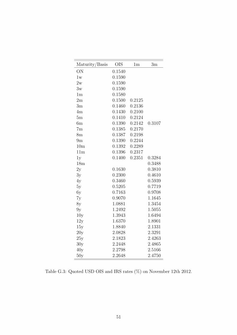
Maturity/Basis OIS 1m 3m

ON 0.15401w 0.15902w 0.15903w 0.15901m 0.15802m 0.1500 0.21253m 0.1460 0.21364m 0.1430 0.21005m 0.1410 0.21246m 0.1390 0.2142 0.31077m 0.1385 0.21708m 0.1387 0.21989m 0.1390 0.224410m 0.1392 0.228911m 0.1396 0.23171y 0.1400 0.2351 0.328418m 0.34882y 0.1630 0.38103y 0.2300 0.46104y 0.3460 0.59395y 0.5205 0.77196y 0.7163 0.97087y 0.9070 1.16458y 1.0881 1.34549y 1.2492 1.505510y 1.3943 1.649412y 1.6370 1.890115y 1.8840 2.133120y 2.0828 2.329125y 2.1823 2.426330y 2.2448 2.486540y 2.2798 2.516650y 2.2648 2.4750

Table G.3: Quoted USD OIS and IRS rates (%) on November 12th 2012.

51

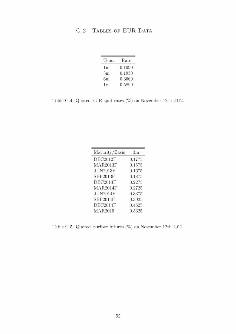
G.2 Tables of EUR Data

Tenor Rate

1m 0.10903m 0.19306m 0.36601y 0.5890

Table G.4: Quoted EUR spot rates (%) on November 12th 2012.

Maturity/Basis 3m

DEC2012F 0.1775MAR2013F 0.1575JUN2013F 0.1675SEP2013F 0.1875DEC2013F 0.2275MAR2014F 0.2725JUN2014F 0.3375SEP2014F 0.3925DEC2014F 0.4625MAR2015 0.5325

Table G.5: Quoted Euribor futures (%) on November 12th 2012.

52

Maturity/Basis 1m/6m 3m/6m 6m/1y

3y 0.2630 0.1530 0.16004y 0.2605 0.1485 0.13905y 0.2580 0.1440 0.12606y 0.2525 0.1395 0.11707y 0.2480 0.1350 0.11008y 0.2430 0.1310 0.10509y 0.2375 0.1265 0.101010y 0.2330 0.1220 0.098011y 0.2265 0.1175 0.096012y 0.2195 0.1125 0.093013y 0.2135 0.1082 0.089814y 0.2084 0.1044 0.086415y 0.2040 0.1010 0.083016y 0.1999 0.0979 0.080017y 0.1959 0.0949 0.077418y 0.1921 0.0922 0.075019y 0.1885 0.0895 0.072920y 0.1850 0.0870 0.071021y 0.1819 0.0847 0.069322y 0.1790 0.0826 0.067823y 0.1765 0.0806 0.066424y 0.1741 0.0787 0.065125y 0.1720 0.0770 0.064026y 0.1698 0.0753 0.063027y 0.1674 0.0737 0.062128y 0.1650 0.0721 0.061329y 0.1625 0.0705 0.060630y 0.1600 0.0690 0.060035y 0.1513 0.0632 0.057240y 0.1456 0.0595 0.055150y 0.1373 0.0540 0.0524

Table G.6: Quoted EUR tenor basis spreads (%) on November 12th 2012.

53

Maturity/Basis OIS 1m 6m

ON 0.03001w 0.08202w 0.08203w 0.08201m 0.08102m 0.0790 0.10903m 0.0720 0.10304m 0.0660 0.09905m 0.0600 0.09406m 0.0550 0.09107m 0.0520 0.08808m 0.0500 0.08709m 0.0490 0.086010m 0.0480 0.085011m 0.0480 0.08501y 0.0480 0.0850 0.343018m 0.09452y 0.0830 0.1259 0.39003y 0.1790 0.49604y 0.3370 0.65705y 0.5330 0.85206y 0.7340 1.05207y 0.9230 1.23908y 1.0910 1.40509y 1.2400 1.551010y 1.3710 1.678011y 1.4910 1.793012y 1.5980 1.894013y 1.6851 1.980014y 1.7671 2.052015y 1.8280 2.108016y 1.8689 2.151017y 1.9013 2.181018y 1.9271 2.202019y 1.9483 2.217020y 1.9670 2.227021y 1.9818 2.235022y 1.9919 2.242023y 1.9990 2.247024y 2.0045 2.251025y 2.0100 2.253026y 2.0146 2.254027y 2.0175 2.255028y 2.0199 2.256029y 2.0227 2.257030y 2.0270 2.260035y 2.0634 2.293040y 2.1314 2.342050y 2.1912 2.4120

Table G.7: Quoted EUR OIS and IRS rates (%) on November 12th 2012.

54

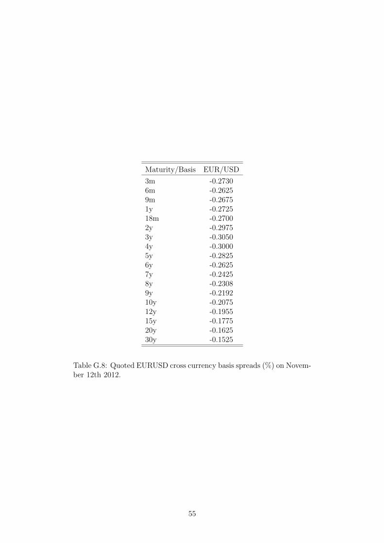
Maturity/Basis EUR/USD

3m -0.27306m -0.26259m -0.26751y -0.272518m -0.27002y -0.29753y -0.30504y -0.30005y -0.28256y -0.26257y -0.24258y -0.23089y -0.219210y -0.207512y -0.195515y -0.177520y -0.162530y -0.1525

Table G.8: Quoted EURUSD cross currency basis spreads (%) on Novem-ber 12th 2012.

55

TRITA-MAT-E 2013:19 ISRN-KTH/MAT/E—13/19-SE

www.kth.se