curve | carleton university research virtual environment
TRANSCRIPT

Energy Optimization forVirtualized Network Environments
by
Ebrahim Ghazisaeedi, M.Sc.
A thesis submitted to the
Faculty of Graduate and Postdoctoral Affairs
in partial fulfillment of the requirements for the degree of
Doctor of Philosophy in Electrical and Computer Engineering
Ottawa-Carleton Institute for Electrical and Computer Engineering
Department of Systems and Computer Engineering
Carleton University
Ottawa, Ontario
August, 2015
c©Copyright
Ebrahim Ghazisaeedi, 2015

Abstract
Information and Communication Technology (ICT) has been estimated to consume
10% of the total energy consumption in industrial countries. According to the latest
measurements, this amount is rapidly increasing by 6% annually. With the evolved
new business model in which Service Providers (SPs) are separated from Infrastruc-
ture Providers (InPs), Virtualized Network Environments (VNEs) have been regarded
as a promising technology for flexibly utilizing shared communication network re-
sources. VNEs also play a fundamental role toward virtualizing data centers. In this
thesis, we suggest different feasible solutions to optimize the energy consumption in
a VNE. In this regard, first, we review the corresponding literature in regard to the
architecture of a VNE, its performance modelling, several power models, and also
existing energy-saving solutions for VNEs. We approach the objective of optimizing
the energy consumption in a VNE by defining and solving two main problems. The
first problem optimizes the energy consumption in a VNE during the off-peak period.
This is feasible by reconfiguring the mapping of already embedded virtual networks
for the off-peak time. This is planned in two smaller and simpler sub-problems with
increasing the complexity and higher energy-saving levels. Our solutions enable the
providers to adjust the level of the reconfiguration and accordingly control the pos-
sible traffic disruptions. In the second problem, we propose a novel energy-efficient
embedding method that maps heterogeneous MapReduce-based virtual networks onto
a heterogeneous data center physical network, energy-wise. We introduce a new in-
cast problem that specifically may happen in Virtualized Data Centers (VDCs). The
proposed embedding process also controls the incast queueing delay.
ii

To my parents
iii

Acknowledgments
I would like to express my special appreciation and thanks to my supervisor Professor
Changcheng Huang, he has been a tremendous mentor for me. I would like to thank
him for encouraging my research and for allowing me to grow as a research scientist.
His advice on both research as well as on my career have been priceless.
I would like to thank Professors Pin-Han Ho, Yiqiang Zhao, Richard Yu, and
Hussein Mouftah for their careful review and contributions to the thesis.
A special thanks to my family. Words cannot express how grateful I am to my
mother, father, and my sister, for all of the sacrifices that they have made on my
behalf. Their prayer for me was what sustained me thus far. I would also like to
thank all of my friends who supported me in writing, and incented me to strive
towards my goal.
iv

Contents
Abstract ii
Acknowledgments iv
Table of Contents v
List of Tables viii
List of Figures ix
Acronyms xii
Terms and Definitions xv
1 Introduction 1
1.1 Motivation . . . . . . . . . . . . . . . . . . . . . . . . . . . . . . . . . 1
1.2 Objective and Scope . . . . . . . . . . . . . . . . . . . . . . . . . . . 3
1.3 Contributions . . . . . . . . . . . . . . . . . . . . . . . . . . . . . . . 5
1.4 Publications . . . . . . . . . . . . . . . . . . . . . . . . . . . . . . . . 8
1.5 Organization of Thesis . . . . . . . . . . . . . . . . . . . . . . . . . . 9
2 Literature Review 10
2.1 Structure of Virtualized Network Environments . . . . . . . . . . . . 11
2.2 Modelling and Analysis of VNEs . . . . . . . . . . . . . . . . . . . . 14
2.2.1 VNE Embedding Problems . . . . . . . . . . . . . . . . . . . . 14
2.2.2 Network Performance in VNEs . . . . . . . . . . . . . . . . . 33
2.2.3 Performance Modelling of Virtualized Servers . . . . . . . . . 42
2.3 Energy-Saving for VNEs . . . . . . . . . . . . . . . . . . . . . . . . . 45
2.3.1 Node Power Models . . . . . . . . . . . . . . . . . . . . . . . . 46
v

2.3.2 Link Power Models . . . . . . . . . . . . . . . . . . . . . . . . 52
2.3.3 Existing Energy-Saving Solutions for VNEs . . . . . . . . . . 57
3 Off-Peak Energy Optimization for Links in a VNE 61
3.1 Introduction . . . . . . . . . . . . . . . . . . . . . . . . . . . . . . . . 61
3.2 Power Models . . . . . . . . . . . . . . . . . . . . . . . . . . . . . . . 65
3.3 Integer Linear Programs . . . . . . . . . . . . . . . . . . . . . . . . . 66
3.3.1 The Network Model . . . . . . . . . . . . . . . . . . . . . . . 67
3.3.2 Programs based on Fixed Link Power Model . . . . . . . . . . 68
3.3.3 Programs based on Semi-Proportional Link Power Model . . . 77
3.4 The Heuristic Algorithm . . . . . . . . . . . . . . . . . . . . . . . . . 78
3.5 Evaluation . . . . . . . . . . . . . . . . . . . . . . . . . . . . . . . . . 81
3.5.1 ILPs . . . . . . . . . . . . . . . . . . . . . . . . . . . . . . . . 83
3.5.2 The Heuristic . . . . . . . . . . . . . . . . . . . . . . . . . . . 86
3.6 Summary . . . . . . . . . . . . . . . . . . . . . . . . . . . . . . . . . 94
4 Off-Peak Energy Optimization for Nodes and Links in a VNE 95
4.1 Introduction . . . . . . . . . . . . . . . . . . . . . . . . . . . . . . . . 95
4.2 Power Models . . . . . . . . . . . . . . . . . . . . . . . . . . . . . . . 98
4.3 Integer Linear Programs . . . . . . . . . . . . . . . . . . . . . . . . . 99
4.3.1 The Network Model . . . . . . . . . . . . . . . . . . . . . . . 101
4.3.2 Programs Based on Fixed Power Model . . . . . . . . . . . . . 102
4.3.3 Programs Based on Semi-Proportional Power Model . . . . . . 119
4.4 The Heuristic Algorithm . . . . . . . . . . . . . . . . . . . . . . . . . 120
4.5 Evaluation . . . . . . . . . . . . . . . . . . . . . . . . . . . . . . . . . 124
4.5.1 ILPs . . . . . . . . . . . . . . . . . . . . . . . . . . . . . . . . 126
4.5.2 The Heuristic . . . . . . . . . . . . . . . . . . . . . . . . . . . 134
4.6 Summary . . . . . . . . . . . . . . . . . . . . . . . . . . . . . . . . . 141
5 GreenMap: Green Mapping of Heterogeneous MapReduce-based
Virtual Networks onto a Data Center Network and Controlling In-
cast Queueing Delay 142
5.1 Introduction . . . . . . . . . . . . . . . . . . . . . . . . . . . . . . . . 142
5.2 The Network Model . . . . . . . . . . . . . . . . . . . . . . . . . . . . 146
5.3 Power Models . . . . . . . . . . . . . . . . . . . . . . . . . . . . . . . 148
vi

5.4 The Mixed Integer Disciplined Convex Program . . . . . . . . . . . . 149
5.5 The Heuristic Algorithm . . . . . . . . . . . . . . . . . . . . . . . . . 157
5.6 Evaluation . . . . . . . . . . . . . . . . . . . . . . . . . . . . . . . . . 169
5.6.1 The MIDCP . . . . . . . . . . . . . . . . . . . . . . . . . . . . 171
5.6.2 The Heuristic . . . . . . . . . . . . . . . . . . . . . . . . . . . 175
5.7 Summary . . . . . . . . . . . . . . . . . . . . . . . . . . . . . . . . . 180
6 Conclusion and Future Works 181
6.1 Off-Peak Energy Optimization for a VNE . . . . . . . . . . . . . . . . 181
6.2 GreenMap . . . . . . . . . . . . . . . . . . . . . . . . . . . . . . . . . 183
List of References 185
vii

List of Tables
2.1 Node and link attributes in VNEs . . . . . . . . . . . . . . . . . . . . 20
2.2 Parameters of physical link power consumption . . . . . . . . . . . . 53
4.1 Re-allocation combinations for virtual nodes of lam,bmn , and the required
off-peak traffic to be rerouted . . . . . . . . . . . . . . . . . . . . . . 107
viii

List of Figures
2.1 A Virtualized Network Environment . . . . . . . . . . . . . . . . . . 11
2.2 A VNE embedding process . . . . . . . . . . . . . . . . . . . . . . . . 12
2.3 M/M/1 queue model for non-virtualized severs . . . . . . . . . . . . . 42
2.4 Queue model for virtual servers [1] . . . . . . . . . . . . . . . . . . . 44
2.5 Two dimensional Markov-Chain model for two virtualized severs on a
single physical server [1] . . . . . . . . . . . . . . . . . . . . . . . . . 45
2.6 Three types of power models . . . . . . . . . . . . . . . . . . . . . . . 47
3.1 Example: An embedded virtual link onto a substrate network . . . . 68
3.2 Example: Generated random topologies . . . . . . . . . . . . . . . . . 82
3.3 Off-peak link energy optimization by global link reconfiguration vs.
local link reconfiguration (splittable traffic) . . . . . . . . . . . . . . . 83
3.4 (a) The total link power consumption of off-peak link energy optimiza-
tion by global link reconfiguration. (b) The total link power consump-
tion of off-peak link energy optimization by local link reconfiguration
for splittable traffic. (c) The total link power consumption of off-peak
link energy optimization by local link reconfiguration for non-splittable
traffic. . . . . . . . . . . . . . . . . . . . . . . . . . . . . . . . . . . . 84
3.5 The total saved power with off-peak link energy optimization by local
link reconfiguration for splittable and non-splittable traffic . . . . . . 86
3.6 The BILP vs. the heuristic for off-peak link energy optimization by
local link reconfiguration (non-splittable traffic) . . . . . . . . . . . . 87
3.7 The total link power consumption of the heuristic for off-peak link
energy optimization by local link reconfiguration . . . . . . . . . . . . 88
3.8 The link reconfiguration heuristic for the different numbers of involved
VNs . . . . . . . . . . . . . . . . . . . . . . . . . . . . . . . . . . . . 89
3.9 The effect of changing the stress rate threshold on the heuristic’s outcome 90
3.10 The link reconfiguration heuristic vs. our previous algorithm . . . . . 91
ix

3.11 The mean link utilization over different configurations . . . . . . . . . 91
3.12 The total link power consumption before and after applying the heuris-
tic on the GEANT simulation setup . . . . . . . . . . . . . . . . . . . 92
3.13 The run time for different methods . . . . . . . . . . . . . . . . . . . 93
4.1 The total node and link power consumption based on the off-peak ratio
by the MILPs for ONL-LNLs-F and ONL-LNLs-SP . . . . . . . . . . 127
4.2 The total saved power in the network, the total saved power in physical
nodes, and the total saved power in physical links based on the off-peak
ratio by the MILP for ONL-LNLs-F . . . . . . . . . . . . . . . . . . . 128
4.3 The total node and link power consumption based on the off-peak ratio
by the MILPs for ONL-LLs-F and ONL-LLs-SP . . . . . . . . . . . . 128
4.4 The total node and link power consumption based on the off-peak ratio
by the BILPs for ONL-LLns-F and ONL-LLns-SP . . . . . . . . . . . 129
4.5 The total saved power in physical nodes and links based on the off-peak
ratio by the MILPs for ONL-LNLs-F and ONL-LLs-F . . . . . . . . . 130
4.6 The total saved power in physical nodes and links based on the off-peak
ratio by the ILPs for ONL-LLs-F and ONL-LLns-F . . . . . . . . . . 131
4.7 The total saved power in physical nodes and links based on the off-peak
ratio by the MILPs for ONL-LLs-F and ONL-LLs-SP . . . . . . . . . 131
4.8 The total saved power in physical nodes and links based on the number
of involved virtual networks by the MILP for ONL-LLs-F . . . . . . . 132
4.9 The total saved power in physical nodes and links based on the number
of virtual nodes per VN by the MILP for ONL-LLs-F . . . . . . . . . 133
4.10 The total node and link power consumption based on the off-peak ratio
before and after applying the heuristic with different values of K, for
ONL-LLns-F . . . . . . . . . . . . . . . . . . . . . . . . . . . . . . . 135
4.11 The total saved power in physical nodes and links based on the off-
peak ratio by the BILP and the heuristic with different values of K,
for ONL-LLns-F . . . . . . . . . . . . . . . . . . . . . . . . . . . . . . 136
4.12 The total saved power in physical nodes and links based on the number
of involved virtual networks by the heuristic with K = 5, for ONL-
LLns-F . . . . . . . . . . . . . . . . . . . . . . . . . . . . . . . . . . . 137
4.13 The total saved power in physical nodes and links based on the number
of virtual nodes per VN by the heuristic with K = 5 for ONL-LLns-F 137
x

4.14 The impact of different s2 thresholds on the total saved power in phys-
ical nodes and links by the heuristic when K = 5 for ONL-LLns-F . . 138
4.15 Comparison between the suggested heuristic in this chapter and pre-
viously proposed heuristic in Chapter 3 . . . . . . . . . . . . . . . . . 139
4.16 The mean link utilization based on the off-peak ratio over different
configurations . . . . . . . . . . . . . . . . . . . . . . . . . . . . . . . 139
4.17 Required run time based on the different number of virtual nodes per
VN, for the BILP and the heuristic with K = 5, for ONL-LLns-F . . 140
5.1 Example: A MapReduce-based VN’s topology . . . . . . . . . . . . . 147
5.2 The heuristic’s decision making process . . . . . . . . . . . . . . . . . 163
5.3 Topology of the data center network in a small simulation setup . . . 169
5.4 The total power consumption based on different numbers of virtual
nodes per VN for the state-of-the-art algorithm, the MIDCP for Green-
Map, and the heuristic for GreenMap . . . . . . . . . . . . . . . . . . 172
5.5 The mean incast queueing delay based on different CPU demands of a
computation-based virtual node for the MIDCP, as well as the chosen
maximum tolerable queueing delay D for a virtual link . . . . . . . . 173
5.6 The total VDC’s power consumption based on different CPU demands
of a computation-based virtual node for the MIDCP, and the MIDCP
when the incast constraints are relaxed . . . . . . . . . . . . . . . . . 174
5.7 The total VDC’s power consumption based on different numbers of vir-
tual nodes per VN for the state-of-the-art algorithm, and the heuristic
for GreenMap . . . . . . . . . . . . . . . . . . . . . . . . . . . . . . . 176
5.8 The mean inast queuing delay based on different numbers of virtual
nodes per VN for the heuristic for GreenMap, as well as the maximum
tolerable queuing delay D for a virtual link . . . . . . . . . . . . . . . 177
5.9 The mean acceptance ratio based on different values of D for the heuris-
tic for GreenMap . . . . . . . . . . . . . . . . . . . . . . . . . . . . . 178
5.10 The mean acceptance ratio based on different mean traffic rates of a
mapper virtual node for the heuristic for GreenMap . . . . . . . . . . 179
5.11 The mean incast queuing delay based on different mean traffic rates of
a mapper virtual node for the heuristic for GreenMap . . . . . . . . . 179
xi

Acronyms
BILP Binary Integer Linear Program
BT British Telecom
CPU Central Processing Unit
GeSI Global e-Sustainability Initiative
ICT Information and Communication Technology
IP Internet Protocol
ISP Internet Service Provider
InP Infrastructure Provider
ILP Integer Linear Program
LSP Label-Switched Path
MPLS Multi Protocol Label Switching
MTU Maximum Transmission Unit
MIB Management Information Base
MIDCP Mixed Integer Disciplined Convex Program
MMPP Markov Modulated Poisson Process
MILP Mixed Integer Linear Program
NF Non-functional
ON Overlay Networks
OL-GLs-F Off-peak Link energy optimization by Global Link reconfiguration,Splittable traffic, Fixed power model
xii

OL-GLs-SP Off-peak Link energy optimization by Global Link reconfiguration,Splittable traffic, Semi-Proportional power model
OL-LLs-F Off-peak Link energy optimization by Local Link reconfiguration,Splittable traffic, Fixed power model
OL-LLs-SP Off-peak Link energy optimization by Local Link reconfiguration,Splittable traffic, Semi-Proportional power model
OL-LLns-F Off-peak Link energy optimization by Local Link reconfiguration,Non-Splittable traffic, Fixed power model
OL-LLns-SP Off-peak Link energy optimization by Local Link reconfiguration,Non-Splittable traffic, Semi-Proportional power model
ONL-LNLs-F Off-peak Node and Link energy optimization by Local Node andLink reconfiguration, Splittable traffic, Fixed power model
ONL-LNLs-SP Off-peak Node and Link energy optimization by Local Node andLink reconfiguration, Splittable traffic, Semi-Proportional powermodel
ONL-LLs-F Off-peak Node and Link energy optimization by Local Link recon-figuration, Splittable traffic, Fixed power model
ONL-LLs-SP Off-peak Node and Link energy optimization by Local Link recon-figuration, Splittable traffic, Semi-Proportional power model
ONL-LLns-F Off-peak Node and Link energy optimization by Local Link recon-figuration, Non-Splittable traffic, Fixed power model
ONL-LLns-SP Off-peak Node and Link energy optimization by Local Link recon-figuration, Non-Splittable traffic, Semi-Proportional power model
QoS Quality of Service
RTT Round Trip Time
RTO Retransmission Timeout
SP Service Provider
SLO Service Level Objective
SLA Service Level Agreement
SDN Software-defined Networking
TCP Transmission Control Protocol
ToR Top-of-Rack
xiii

UDP User Datagram Protocol
VDC Virtualized Data Center
VNE Virtualized Network Environment
VN Virtual Network
VM Virtual Machine
VLAN Virtual Local Area Network
VPN Virtual Private Network
WDM Wavelength-Division Multiplexing
xiv

Terms and Definitions
A(.) A node/link’s attribute
A(.) Attribute of an allocated virtual resource
α(.) Status of a node/link
α(., .) A binary variable denotes whether a virtual node is allocated in a sub-strate node or not
α(.) A node/link’s status before embedding
α(.) A node/link’s status after embedding
b(.) Blocking probability
β(.) Status of a traffic capacity, after reconfiguration
B A large number
c(.) Cost
cc(.) Congestion cost
C(.) Capacity
C(.) Requested capacity
Cb(.) Requested bandwidth capacity
Cc(.) Requested processing capacity
Cmc (.) Minimum amount of required CPU capacity per allocated physical ma-
chine for a computation-based virtual node
Cmc (.) Maximum amount of required CPU capacity per allocated physical ma-
chine for a computation-based virtual node
C(.) Allocated capacity
xv

Cc(.) Off-peak processing demand
C i,jb (.) Allocated traffic capacity in li,js to a virtual link, or bundled allocated
traffic capacity in li,js
Cc(.) Allocated processing capacity
Cb(.) Available bandwidth capacity
Cc(.) Available processing capacity
Cb(.) Bandwidth capacity
Cc(.) CPU capacity
Ci(., .) Minimum incast processing capacity
d Delay/Latency
dp(.) Propagation delay
dq(.) Queuing delay
D Maximum tolerable queuing delay in a virtual link
di,jn (m) An intermediate optimization variable
dx,yn (m) Fraction of Cb(lam,bm
n ) that needs to be allocated to lx,yn (m)
di,j(lx,yn (m)) Amount of allocated traffic capacity to lx,yn (m) in li,js
Δi,j Dissimilarity function of all the attributes between ith node and jth node
Δi,jm Dissimilarity of mth attribute between ith node and jth node
Es Set of edges in a substrate network graph
En Set of edges in nth VN graph
Emv Set of edges of the involved VN with the largest number of virtual links
η(.) Number of involved VNs in a substrate node/link
E(t) Departed traffic load from a service component by time t
Φ Set of all the involved VNs
f i,jn (m) Re-allocated traffic capacity in li,js to lam,bm
n (may be part of link recon-figuration sub-problem)
xvi

f ′i,jn (m) Re-allocated traffic capacity in li,js to lam,bm
n (part of node reconfigurationsub-problem)
f i,j(Cx,yb ) Re-allocated traffic capacity in li,js to Cx,y
b
φ(., .) Status of an allocated virtual node/link in a substrate node/link
φ(., .) Fraction of processing/switching demand of a virtual node that is allo-cated in a substrate node
φ(., .) Re-allocation status of an allocated virtual node/link in a substratenode/link
φ(.) Total allocated processing capacity to virtual nodes in a substrate node
Gs Substrate network graph
Gn nth virtual network graph
gf(.) General objective function to be defined based on the traffic classes
H Hessian matrix
Ht Header of Transport layer
Hi Header of IP layer
h(.) Traffic scalability factor
κi,jm Priority coefficients of mth attribute between ith node and jth node
K Number of shortest paths
Ls Total number of substrate links
li,js Substrate link that connects ith substrate node to jth substrate node
Ln Total number of virtual links in nth VN
la,bn Virtual link belonging to nth virtual network, connects ath virtual nodeto bth virtual node
lam,bmn mth virtual link in nth virtual network, connects the virtual node
mapped onto amth substrate node to the virtual node mapped onto bmthsubstrate node
lx,yn (m) A sub virtual link of lam,bm
n that connects the allocated source virtualnode in vxs to the allocated sink virtual node in vys
L(.) Set of substrate link candidates
xvii

l(.) Loss rate
L(li,js , t) Number of virtual links allocated in li,js at time t
L Number of physical links in the found longest substrate path
λ Arrival mean rate
λMn Summation of arrival rates of all mappers in nth VN
λ Waxman parameter
L(.) Set of adjacent links
L(t) Traffic load function
μ Service mean rate
μ Waxman parameter
M The largest virtual link bandwidth demand in Φ
Ns Total number of substrate nodes
Nn Total number of virtual nodes in nth VN
N(.) Set of substrate node candidates
N(vis, t) Number of virtual nodes allocated in vis at time t
Oo Overhead of overlay networks
Oe Overhead of Ethernet
Oi Overhead of IP layer
Ot Overhead of Transport layer
OT Total overheads
ωmn A binary variable to show the status of intermediate substrate nodes over
the allocated substrate path to lam,bmn
ωmn A binary variable to show the reconfiguration status of the relay nodes
of lam,bmn
ωmn A binary variable to show the reconfiguration status of the source and
sink nodes of lam,bmn
pi,js Substrate path that connects ith substrate node to jth substrate node
xviii

pTs Set of all possible paths in a substrate network
p′s Sub-set of substrate paths
pa,bn Substrate path which la,bn is mapped onto
ψ Tuneable weight
P (j) Probability of being in state j
p(.) Power consumption of a link or node
pb(.) Base power consumption
pm(.) Maximum power consumption
pc(.) Power consumption of the unit CPU utilization in the unit time
pe(.) Power consumption of a packet processor engine
ql(.) Queue length
r(.) Revenue
ru Revenue earned per carried call per unit time
r(.) Traffic rate
r Mean traffic rate
rmn Off-peak traffic demand of lam,bmn
ri,jn (m) Off-peak traffic demand of lam,bmn in li,js
ri,jb Bundled off-peak traffic demand in li,js
RTTL Longest RTT
ρ Traffic intensity
R(t) Arrival traffic load to the service component by time t
s(.) Stress rate
sp Packet Size
sl Payload size
S(t) Traffic capability function
xix

Si(t) ith traffic capability function
Se(t) End-to-end traffic capability function
S L Sorted list of nodes/links
σ Standard deviation
T Stress rate’s treshold
U(.) Node/Link utilization
Uc(.) CPU utilization
Υi,j jth port of ith router
Υ Set of router ports corresponding to the considered LSP
|Υi| Number of line cards in ith router
Vs Set of vertices in a substrate network graph
Vs Set of server nodes in a substrate network
Vs Set of switch/router substrate nodes in a substrate network
V ′s Sub-set of substrate nodes
vis ith substrate node
vis ith substrate node that is a server
vis ith substrate node that is a switch/router
Vn Set of vertices in nth VN graph
Vn Set of mapper virtual nodes in nth VN
Vn Set of reducer virtual nodes in nth VN
Vn Set of shuffler virtual nodes in nth VN
vkn kth virtual node in nth VN
vkn kth virtual node that is a mapper, in nth VN
vkn kth virtual node that is a reducer, in nth VN
vkn kth virtual node that is a shuffler, in nth VN
xx

Vkn(i) Removable amount of allocated processing capacity to vkn in vis
V ′kn Total removable amount of allocated processing capacity to vkn
V∗kn Total removed processing capacity for vkn
�mn (vis) Status of vis over the allocated substrate path to lam,bm
n
�′mn (vis) Status of vis, that is a relay node, over the allocated substrate path to
lam,bmn
W (.) Weight
x An average result
ζ Base power consumption ratio
zi,j(.) Status of a re-allocated commodity in li,js
zi,jn (m) Re-allocation status of lam,bmn in li,js
xxi

Chapter 1
Introduction
1.1 Motivation
Nowadays, Information and Communication Technology (ICT) plays a fundamental
role in everyday life of individuals. It is difficult to imagine a world without the
infrastructure that connects people and transfers their information across the globe.
Significant advantages of communication networks have stimulated the demand for
this technology. It is predicted that the size of the Internet network doubles every
5.32 years [2]. The increase in population’s demand, spreading of broadband access
and the new services offered by ICT, have triggered the warnings about the energy
consumption of the communication technology [3]. The ICT’s energy consumption is
important to the world due to two main reasons [4]:
1. The environmental reason. It is needed to reduce wastes for controlling CO2
emission.
2. The cost reason. The operators would like to provide services with the min-
imum cost. However, the cost of energy is high, so by decreasing the energy
consumption they can pay less for the energy.
Several reports from different ICT organizations over the world confirm the in-
creasing demand of energy in this technology, which is a concern. In the case
that no green technology would be deployed in communication networks, Global e-
Sustainability Initiative (GeSI) predicts 35.8TWh energy consumption for European
telecom operators in 2020, while they have already consumed 21.4TWh in 2010 [5].
The European Commission DG INFSO has the similar estimation and predicts an
1

CHAPTER 1. INTRODUCTION 2
energy consumption of 35.8TWh for ICT in 2020 if no green network technologies
would be used [6]. Besides, Deutsche Telekom in [7] stated 2% increase in the total
energy consumption from year 2006 to 2007, due to the technology developments, in-
creasing transmission volumes and network expansions. In addition, British Telecom
(BT) reported 2.5TWh energy consumption for its networks over the 2008 financial
year [8]. This happens while the ICT related devices, in 2007, have consumed about
10% of the United Kingdom’s energy consumption [9]. This problem is even worse
when we consider servers and data center clusters. The volume of data needed to be
processed by servers in data centers is increasing every day [10], and consequently the
energy consumption of their infrastructure is growing. The data centers are estimated
to consume 1.4% of the worldwide electricity energy consumption, while this grows
with the rate of 12% per year [11]. These infrastructures in USA have consumed 61
billion KWh for a cost of 4.5 billion dollars in 2006 [12]. In Amazon’s data centers,
53% of the total budget, over 15 years period, has been used for the operation of
servers, while 42% of the total budget has been considered for the energy-related
costs. This includes 19% of the direct energy consumption and 23% for the cooling
infrastructure [13]. All the cited reports show the growing energy consumption in
ICT, which confirms the necessity of implementing energy-saving mechanisms in this
technology. Consequently, it is vital to study and design effective methods that not
only control the rapidly increasing energy consumption, but also save the energy.
Recently, virtualization has been proposed to share resources in a network envi-
ronment [14]. A Virtualized Network Environment (VNE) supports the coexistence
of multiple Virtual Networks (VNs) over a single physical network [15]. A VNE
embedding process maps virtual nodes and links onto physical nodes and paths, re-
spectively. A VNE uses the actual resources more efficiently by sharing a physical
network’s capacity among multiple virtual networks. Each virtual network is iso-
lated from others, and might run its desired network protocols and services. Network
virtualization decouples the functionality of the current networks’ architecture into
Infrastructure Providers (InPs) and Service Providers (SPs). Besides, Virtual Ma-
chines (VMs) traditionally virtualize physical servers’ resources. VNs together with
the VMs underpin Virtualized Data Centers (VDCs). Traditional data centers are
moving toward virtualized data centers in order to address cloud computing limita-
tions regarding the network performance, security, and manageability [16]. Hence,
network virtualization has been regarded as a promising technology to flexibly share

CHAPTER 1. INTRODUCTION 3
the resources, and therefore the corresponding solutions to energy-saving in this type
of network become essential.
However, as far as energy efficiency is concerned, few research works have con-
sidered energy-saving in virtualized network environments. A VNE needs distinct
energy-saving solutions that are designed specially for its architecture. In a VNE
embedding process, it is required to map both virtual nodes and virtual links onto
the substrate network. This is more complex than non-virtualized networks in which
nodes are fixed. Besides, virtual network demands do not necessarily mean the same
as current demands [17]. VN demands are the capacities that the virtual network
customers ask from the SPs. They are the upper bounds of the demands generated,
processed, and transported by a VN. Hence, in an allocated virtual network, further
energy optimization can be carried out applying any of the existing energy-saving
techniques [17]. Moreover, allocated virtual networks might have different quality of
service requirements, so it is not possible to treat all of them in a similar way. For
instance, imagine two virtual links that are mapped onto a physical link. The first
virtual link is a part of a virtual network that is throughput-sensitive. However, the
second virtual link belongs to another virtual network that is delay-sensitive. It is
not efficient to treat all the traffic in the physical link similarly.
1.2 Objective and Scope
According to the discussion in Section 1.1, the main objective of this thesis is to
develop new energy-saving solutions for a virtualized network environment. Multiple
fundamental steps are required to be taken toward this objective.
First, we study the architecture of a VNE to give a clear understanding of its
evolved structure. It also helps to discover any possible opportunities to save the
energy in such an environment. We also review different studies in the literature in
regard to modelling a VNE embedding process, and analyzing its performance. Ac-
curate knowledge of a VNE’s architecture and its processes, prepares us to discover
energy-saving opportunities in this environment. The main energy consumers in a
VNE are physical network elements. Power models of different physical nodes and
links, as of the two most important physical network elements, are reviewed. The
power models determine the factors affect the energy consumption of the network
elements, so we can save the energy more effectively by targeting them. A VNE does

CHAPTER 1. INTRODUCTION 4
not change physical power models provided for non-virtualized networks, because the
a substrate network is still the main energy consumer in its architecture. Nonethe-
less, mapping virtual networks onto a physical network might increases the substrate
network’s energy consumption. As far as energy efficiency is concerned, very few
research works have considered energy-saving in virtualized network environments.
In this regard, the literature is surveyed regarding existing energy-saving solutions
for VNEs. We study their advantages and disadvantages. We also discuss the open
research areas.
According to the open research areas, we plan to approach the objective by defin-
ing and solving two main problems. The first problem optimizes the energy consump-
tion in a VNE during the off-peak time, by reconfiguring the mapping of embedded
VNs once networks go from the peak time to the off-peak time. This problem is
planned in two smaller and simpler sub-problems with increasing the complexity and
higher energy-saving levels.
Due to the simpler technical implementation and the high potential of energy-
saving in network links, the first sub-problem in the first problem is restricted to
energy-saving solutions for links in a VNE. It reconfigures the mapping of virtual links
according to the off-peak traffic demands. We formulate multiple novel energy-saving
reconfiguration methods that globally/locally optimize the link energy consumption
in VNE during the off-peak time. The proposed fine-grained local reconfiguration
enables the providers to adjust the level of the reconfiguration, and accordingly control
the possible traffic disruptions. An Integer Linear Program (ILP) is formulated for
each solution according to two power models, and considering the impact of traffic
splittability. Because the formulated ILPs are not scalable to large network sizes, a
novel heuristic algorithm is also suggested. The proposed solutions have been verified
through extensive simulations.
Because physical nodes are also essential energy consumers in VNEs, in the second
sub-problem of the first problem, we discuss multiple energy-saving solutions that
locally optimize the node and link energy consumption in a VNE, during the off-
peak period, by reconfiguring the mapping of already allocated virtual nodes and
links. The proposed reconfigurations enable the providers to adjust the level of the
reconfiguration, and accordingly control the possible traffic disruptions. An ILP is
formulated for each solution, according to two power models, and considering the
impact of traffic splittability. Because the defined ILPs areNP-hard, a novel heuristic

CHAPTER 1. INTRODUCTION 5
algorithm is also suggested. The proposed energy-saving methods are evaluated over
random VNEs.
In the second problem, we propose GreenMap, a novel energy-efficient embedding
method that maps heterogeneous MapReduce-based virtual networks onto a heteroge-
neous data center network. Besides, we introduce a new incast problem that specially
may happen in VDCs. GreenMap also controls the incast queueing delay. We formu-
late a Mixed Integer Disciplined Convex Program (MIDCP) for this method. Because
the formulated MIDCP is NP-hard, we also propose a novel and scalable heuristic
for GreenMap. We evaluate GreenMap through extensive simulations.
1.3 Contributions
The contributions of this thesis are:
1. We propose different methods for reconfiguring the mapping of virtual links
during off-peak time, to optimize the off-peak energy consumption of links in a
VNE.
(a) We propose global and local optimization programs in form of ILPs for
this problem.
(b) The solutions are formulated according to two power models.
(c) A coarse-grained and a fine-grained reconfiguration method are suggested
for this problem.
(d) We discuss how differently we should approach the problem in the case
of non-splittable traffic in comparison to splittable traffic, to have a wide
enough search zone for re-mapping.
(e) We also present a heuristic reconfiguration algorithm that could achieve
closely to the optimum results, but much faster than the optimization
solution.
(f) Our methods do not decrease the network admittance ratio for new virtual
networks.
(g) We define a stress rate for a substrate link. So, our solutions enable the
providers to change the level of the reconfiguration by adjusting the stress
rate’s threshold, and therefore control the possible interruptions.

CHAPTER 1. INTRODUCTION 6
(h) Our solutions are not limited to a sub-topology.
(i) We evaluate the proposed solutions by extensive simulations, and study
the impact of different factors.
(j) The simulation results prove that the significant improvement in saving
power by our method in comparison to the state-of-the-art.
(k) To the best of our knowledge, there is not such a comprehensive
study in the literature that considers simultaneously a global/local,
coarse-grained/fine-grained energy-efficient reconfiguration of a VNE for
splittable/non-splittable traffic, according to two power models.
2. We suggest multiple solutions that formulate unique off-peak energy-saving re-
configuration strategies for nodes and links in a VNE.
(a) We propose a local optimization program in form of an MILP that re-
configures the mapping of both virtual nodes and link during the off-peak
time, to optimize the total energy consumption of nodes and links in a
VNE in that period.
(b) We propose local optimization programs in form of ILPs that reconfigure
the mapping of virtual links during the off-peak time, to optimize the
energy consumption of intermediate substrate nodes and substrate links in
a VNE in that period.
(c) The solutions are formulated according to two power models.
(d) Different programs are formulated for splittable and non-splittable traffic
in order to study the impact of traffic splittability.
(e) We present a scalable heuristic algorithm that can achieve closely to the
optimum results, but considerably faster than the optimization program.
(f) Our methods do not decrease the network admittance ratio for new virtual
networks.
(g) We define different stress rates for distinct types of substrate nodes. There-
fore, different from any related research studies, the proposed methods en-
able the providers to control the level of reconfiguration and possible traffic
interruptions.
(h) Our solutions are not limited to a sub-topology, and therefore they have a
larger degree of freedom to save the energy.

CHAPTER 1. INTRODUCTION 7
(i) We assess the impact of different parameters on the energy-saving capa-
bility of the discussed solutions, through extensive simulations.
(j) To the best of our knowledge, these problems are not defined and formu-
lated mathematically in any published studies.
3. We also propose GreenMap, a novel energy-efficient embedding method that
maps heterogeneous MapReduce-based virtual networks onto a heterogeneous
data center network.
(a) GreenMap is formulated as a MIDCP.
(b) A novel and scalable heuristic is also proposed for the problem that can
achieve closely to the optimum points.
(c) Our approach makes it probable to split and map computation-based
virtual nodes onto a data center network. Accordingly, it enables the
providers to embed computation-based VNs onto a data center network.
(d) GreenMap handles heterogeneity of MapReduce-based VNs and a data
center network.
(e) For the first time, we introduce a new incast problem for virtualized data
centers.
(f) We demonstrate a novel approach that controls the introduced incast
queueing delay.
(g) We tackle the incast problem during the provisioning process. Therefore,
it prevents the incast problem from happening at the first place.
(h) We examine both the MIDCP and the heuristic through extensive simula-
tions, and check impacts of different factors.
(i) We demonstrate how controlling the incast queueing delay may affect the
energy-saving level and the networks’ admittance ratio.
(j) To the best of our knowledge, this is the first study on the energy-efficient
embedding of MapReduce-based virtual networks onto a data center net-
work.

CHAPTER 1. INTRODUCTION 8
1.4 Publications
The sections of this thesis appeared in the following publications:
1. Ebrahim Ghazisaeedi, Changcheng Huang, and James Yan, “Off-Peak Energy-
Wise Link Reconfiguration for Virtualized Network Environment,” In 14th
International Symposium on Integrated Network and Service Management (IM),
IFIP/IEEE, pp. 814-817, Ottawa, 11-15 May 2015.
2. Ebrahim Ghazisaeedi, and Changcheng Huang, “Off-Peak Energy Optimization
for Links in Virtualized Network Environment,” Transactions on Cloud Computing,
IEEE, PP, no. 99, (2015).
3. Ebrahim Ghazisaeedi, and Changcheng Huang, “Energy-Efficient Virtual Link
Reconfiguration for Off-Peak Time,” Accepted for Global Communications Confer-
ence (GLOBECOM): Selected Areas in Communications: Green Communications
and Computing, IEEE, San Diego, CA, 6-10 December 2015.
4. Ebrahim Ghazisaeedi, and Changcheng Huang, “Energy-Aware Node and Link
Reconfiguration for Virtualized Network Environments,” Accepted for Computer
Networks Journal, Special Issue on Communications and Networking in the Cloud
II, Elsevier, (2015).
5. Ebrahim Ghazisaeedi, and Changcheng Huang, “EnergyMap: Energy-Efficient
Embedding of MapReduce-based Virtual Networks and Controlling Incast Queueing
Delay,” Under Review for 15th Network Operations and Management Symposium
(NOMS 2016), IEEE/IFIP, Istanbul, 25-29 April 2016.
6. Ebrahim Ghazisaeedi, and Changcheng Huang, “GreenMap: Green Mapping of
Heterogeneous MapReduce-based Virtual Networks onto a Data Center and Managing
Incast Queueing Delay,” Under Review for Journal on Selected Areas in Communi-
cations: Series on Green Communications and Networking (Issue 2), IEEE, (2015).

CHAPTER 1. INTRODUCTION 9
1.5 Organization of Thesis
The remainder of this thesis is organized as follow: Chapter 2 reviews the literature
in three major sub-sections. First, the structure of a VNE and its different processes
are discussed in Section 2.1. Second, modelling and analysis of a VNE are studied
in Section 2.2. Third, Section 2.3 reviews node and link power models, as well as
the very recent energy-saving researches for VNEs. The problem of off-peak energy
optimization for links in a VNE is described and multiple solutions are proposed in
Chapter 3. Off-peak energy optimization problem for nodes and links in a VNE is
defined and different methods are suggested in Chapter 4. GreenMap is formulated
and solved in Section 5. Finally, the thesis concludes and recommends the future
works in Chapter 6.

Chapter 2
Literature Review
According to Section 1.1, it is vital to develop new energy-saving mechanisms for
virtualized network environments. In order to come up with effective solutions, we
study the corresponding literature in this chapter.
Recently, VNEs have been proposed and attracted researchers’ attention. A virtu-
alized network environment allows coexistence of multiple virtual networks on a single
physical network. In this environment, virtual networks are isolated from each other
and they might run different services and protocols. On one hand, researchers have
studied and analyzed VNEs in different points of view such as a VNE’ architecture,
VNE embedding processes, etc. On the other hand, many energy-saving mechanisms
for different types of communications networks are proposed. Nevertheless, VNEs
and energy-saving techniques have been studied separately, and there are only very
few initial works that concerned about energy efficiency in a VNE.
In this chapter, we review the architecture of a VNE in Section 2.1 to give a clear
picture of its structure. Section 2.2 surveys the literature in regard to modelling and
analysis of VNEs. It reviews VNE embedding processes, which map requested virtual
networks onto a substrate network. Besides, this section studies the network per-
formance in VNEs, and analyzes the performance in virtualized servers. Section 2.3
reviews the energy-saving problem specifically for VNEs. In this section, we discuss
the sources of energy consumption in a VNE, and describe different power models. In
addition, it surveys existing energy-saving solutions for VNEs, their advantages and
disadvantages.
10

CHAPTER 2. LITERATURE REVIEW 11
2.1 Structure of Virtualized Network Environ-
ments
Communication networks and specifically the Internet have became very popular.
This popularity is the biggest impediment to their further growth. Because of a multi-
provider architecture of the Internet, modifications to its design is restricted to simple
updates over network technologies and protocols [14, 18]. Network virtualization has
been proposed as an innovation in the networking to bring a dynamic and flexible
structure in which design modifications are simply possible.
Two Virtual
Networks
Substrate Network
Substrate Link
Virtual Node
Virtual Link
Substrate Node
Figure 2.1: A Virtualized Network Environment
In the case that a networking environment supports coexistence of multiple virtual
networks over a same physical network, it is called a virtualized network environment
[15]. This is shown in Figure 2.1. Virtualization can be achieved by logical separation
and segmentation of nodes and also links. A node can be a server, a switch, or a router.
Hence, as a customer point of view, there is a dedicated network for each customer
while they can run their desired network architecture, protocol, and services. Every
single virtual network consists of virtual nodes and links that are mapped onto an
underlay physical network. This makes a virtualized network environment.
Virtualized network environments cover different technologies. It is possible to
categorize virtual networks in four different types of technologies. Firstly, Virtual
Local Area Networks (VLANs), which contain multiple hosts with a common domain.
VLANs are normally considered as a layer 2 (Data Link) architecture [19]. Secondly,
Virtual Private Networks (VPNs) are the other technology which is covered in VNEs.
A VPN has been implemented over different layers. A layer 3 VPN [20, 21] uses

CHAPTER 2. LITERATURE REVIEW 12
Internet Protocol (IP) or Multi Protocol Label Switching (MPLS), as its network layer
protocol. A layer 2 VPN [22, 23] provides an end-to-end connection using Ethernet,
ATM or Frame Relay layer 2 protocols, and there is also Layer 1 VPNs. Thirdly, active
and programmable networks are considered as an instance of network virtualization
[15]. The programmable networks separate communication hardware from the control
plane [24]. Finally, overlay network creates a virtual topology over a physical topology.
This type of network is implemented in the application layer. Overlay networks are
very popular and used widely due to their applications.
CustomerVirtual Network Query
Service Provider (SP)
Infrastructure Provider (InP)
Substrate Node
Allocated Virtual Node
Virtual Node
Virtual Link
Allocated Virtual Link
Substrate Link
Figure 2.2: A VNE embedding process
VNEs propose decoupling of functionalities by dividing current Internet Service
Providers (ISPs) into Infrastructure Providers (InPs), Service Providers (SPs), and
Virtual Network Users [14,25,26]. These terms are described in the followings:
• Infrastructure Provider: This provider owns the underlay physical substrate
network. It needs to discover its actual physical resources to offer for virtual-
ization.

CHAPTER 2. LITERATURE REVIEW 13
• Service Provider: The service provider is responsible for assigning and allocating
physical resources to virtual network demands.
• Virtual Network User: The VN user request a VN demand from a service
provider. The VN User can be an end-host, a service provider, or a virtual
network provider [27].
In a virtualized network environment, as it is shown in Figure 2.2, a VN user
sends a request to a service provider and asks to map a requested virtual network
onto a physical substrate. The VN request may include different demands like the
minimum Central Processing Unit (CPU) rate and the memory for each virtual node,
the minimum bandwidth and the maximum tolerable delay for each virtual link [28].
Afterwards, the infrastructure provider assists the service provider to assign the re-
quested virtual nodes and links in a specific set of virtual resources extracted from
the actual physical resources [27]. The embedding process occurs in three steps as
follow:
1. Candidate discovery or matching: The infrastructure provider prepares and
sends its actual resources and also virtual resources to the service provider.
Then service provider tries to find a set of candidates from nodes and links which
match the VN query of the VN user. The resources can be all the links and their
bandwidth capacity, all the nodes and their CPU capacity, the memory, ports,
and etc. There are several different techniques in the literature, which help
infrastructure providers to make sure they have discovered all their available
resources and also have the updated network devices’ status.
2. Candidate selection: In the second step, the service provider tries to choose the
best selection of virtual set from found candidates in the first step. In this case,
the best set is defined based on the InP, the SP and the VN user’ constraints.
Different algorithms according to different objectives and constraints have been
proposed in the literature in this regard.
3. Candidate binding: In the final step, the found virtual resources will be allo-
cated/reserved to the VN user [27].
After the embedding process, allocated virtual networks run their own protocols
and services, regardless of other active virtual networks. Note that VNE embedding
processes are also called VNE mapping processes, or provisioning processes.

CHAPTER 2. LITERATURE REVIEW 14
2.2 Modelling and Analysis of VNEs
In VNEs, one of the most important challenges is the embedding or mapping problem.
Section 2.2.1 goes through this problem. For this problem, we model a substrate net-
work, a virtual network, and a mapping process. Multiple VNE embedding methods
are proposed in several papers [28–35]. We study their suggested embedding processes
according to their defined objectives, and review their advantages and disadvantages.
Besides, the virtual network customers and also InPs have specific needs of network
performance which has to be satisfied by the service providers. Consequently, network
performance metrics in VNEs are essential to be studied. The end-to-end service
offered by a virtual network may pass through multiple InPs over a substrate network.
Therefore, it is necessary to model the end-to-end service delivery in a VNE and
study its performance dependence to each of the service components. This subject is
reviewed in 2.2.2. Two most important network performance metrics are throughput
and delay. Throughput and delay for VNEs are also surveyed in 2.2.2.
In addition, servers are one of the essential network elements in the network
virtualization. Performance models for virtualized servers are discussed by benefiting
from the queuing theory in Section 2.2.3. Both non-virtualized and virtualized servers
are modelled in order to make the differences between them more clear.
2.2.1 VNE Embedding Problems
As it is discussed, the role of ISPs has been decoupled into two entities in VNEs, infras-
tructure providers and service providers. Infrastructure providers manage a physical
substrate network and offer physical network resources, while service providers afford
the end-to-end services. When a customer needs a virtual network, it sends its vir-
tual network request to a service provider. Then, the SP makes a candidate list and
chooses the best possible mapping for that specific query, according to the available
physical resources and information received from the InP and the customer. Here is
where the challenge of virtual network embedding comes up. The problem statement
is clear: How should services providers map a virtual network query onto the phys-
ical resources in a substrate network, respect to the virtual and substrate networks’
constraints?
In order to analyze a VNE embedding problem, it is required to formulate three
models. First, it is necessary to have a model for a substrate network, which describes

CHAPTER 2. LITERATURE REVIEW 15
the actual physical network’s topology and its constraints. The model has to include
all the physical constraints and concerns of infrastructure providers. Second, there
should be a model for every virtual network, which reveals the requested virtual
network’s topology and all the customer’s requirements. Finally, we need a model
for the embedding process. The embedding model describes the mapping of virtual
queries onto a physical substrate network, according to the defined objectives and
constraints. In this section, we discuss each of the substrate network model, virtual
network model, and the embedding model.
Several embedding techniques have been proposed for VNEs [28–35], according
to different embedding objectives. A common VNE embedding objective is minimiz-
ing the embedding cost, or maximizing the embedding revenue. Different research
studies define various embedding costs or revenues. Other embedding objectives are
also defined by some studies. We also review some of the existing VNE embedding
techniques and their defined objectives, in this section.
Substrate Network Models
In the majority of papers [28–32, 36] that discuss a VNE embedding problem, a
substrate network Gs is modelled by an undirected/directed graph Gs = (Vs, Es)
including different metrics. Where Vs stands for the substrate graph’s vertices, and
Es denotes its edges. Vertices express nodes and edges refer to links. Ns = |Vs| is thetotal number of substrate nodes in Gs, and Ls = |Es| is the total number of substrate
links in Gs. We might use an undirected graph when all the links in the respective
substrate network are symmetric. So, if there is a substrate link li,js that connects
the ith physical node to the jth physical node with a specific amount of bandwidth
capacity, there is also a substrate link lj,is that connects the jth physical node to
the ith physical node with the same amount of bandwidth capacity. However, when
the substrate network is not symmetric, and therefore the metrics are not the same
in both directions, we might use a directed graph. Here is where the graph theory
comes up and all its prosperities can be helpful. The difference between the substrate
models in different papers is the metrics which are added to the graph in order to
fully express a substrate network’s constraints. We review some of them here.
The authors in [29] added two other parameters to a substrate network
model. They modelled a substrate network with an undirected graph Gs =

CHAPTER 2. LITERATURE REVIEW 16
(Vs, Es, A(Vs), A(Es)). The first two parameters stand for nodes and links of a sub-
strate network. A(Vs) and A(Es) demonstrate node attributes and link attributes,
respectively. The authors in [29] considered the CPU capacity and location for node
attributes, and a link attribute denotes a physical link’s bandwidth capacity. They
also have a parameter that expresses the set of all loopless paths in a substrate net-
work. Choosing the CPU capacity as the most important attribute of substrate nodes
is reasonable, because a portion of a physical node’s CPU capacity will be assigned
to a virtual node and so it is required to express the available CPU capacity amount
in the model. Here, a substrate node is a server or a router. The location is also
important, as the majority of VN queries coming from customers specify the location
of their virtual nodes; this can be a specific city or country. Furthermore, a substrate
link has a limited size of bandwidth capacity and each of the virtual networks requests
a specific amount of bandwidth in their virtual links. Therefore, the most important
attribute for a physical link is the bandwidth capacity.
Ines Houidi and others in [30] represented a substrate network with a weighted
undirected graph. They categorized a substrate network’s attributes in functional and
non-functional ones. The functional attributes state the properties and characteris-
tics of the substrate resources as well as their static metrics like the node type, the
node processor type and the capacity, or the link type, the network interface type and
its location, cost, etc. The node type can be switch or router, and the node capacity
can be defined for CPU and the node network processor. The link type shows the
link virtualization technology and the layer which is virtualized, like VLAN, VPN, or
L3/L2. However, the non-functional attributes in [30] are defined for dynamic param-
eters like the available node CPU capacity, the available node bandwidth capacity,
actual Quality of Service (QoS) parameters and Geographic coordinates. Although
adding functional information like the node type, may help to fully express the ac-
tual network, it might make a complicated model which is hard to analyze. We need
to have enough information in the model to fully express the network, as while as
keeping the model simple enough to analyze.
Jing Lu and Jonathan Turner in [31] also used an undirected graph to model
their substrate network. Nonetheless, the edges in their graph are associated with
their length. The length is used to express the shortest path distance between each
pair of nodes. They also added the location to their graph’s nodes to reveal their
access nodes in which traffic enters and leaves the substrate network. Besides, their

CHAPTER 2. LITERATURE REVIEW 17
substrate network model has an attribute for describing the virtual traffic in form of a
set of general traffic constraints. Each of the constraints is simply an upper bound on
the allowed traffic [31]. The location and the link length are important when we are
discussing routing algorithms and traffic engineering in the network virtualization.
The physical node’s location in regard to finding the access/edge nodes is vital, when
we have more than one underlay substrate network supporting a single end-to-end
service. The dependency of a virtual end-to-end service to each of the underlay
substrate networks will be discussed in Section 2.2.2.
Yong Zhu and Mostafa Ammar in [32] also modelled a substrate network with an
undirected graph. However, based on their requirements they added time stamps for
the links and nodes to use their lifetime in their algorithm. Lifetime may be used
to avoid a network section to get overloaded, while there is an idle section. The
load balancing is considered as the main objective of embedding algorithms in some
studies.
The authors in [28] presented a substrate physical network by a weighted undi-
rected graph. The weight for physical nodes shows the available capacity of the node,
while the weight for the links expresses two non-negative values. It includes an ad-
ditive weight value which denotes the cost and delay of a substrate link, and also
another value which denotes the available bandwidth capacity associated to a physi-
cal link. They derived the bandwidth capacity Cb(pi,js ) for a substrate path pi,js that
connects the ith substrate node to the jth substrate node, by finding the minimal
bandwidth in the substrate links lx,ys along the substrate path. This is calculated
in Equation 2.1. They also measured the weight W (pi,js ) (it can be related to cost,
delay, or jitter) for a substrate path pi,js , by finding sum of the weights W (lx,ys ) for the
substrate links lx,ys along the substrate path pi,js . This is calculated in Equation 2.2.
Cb(pi,js ) = min
(x,y)∈pi,js
Cb(lx,ys ) (2.1)
W (pi,js ) =∑
(x,y)∈pi,js
W (lx,ys ) (2.2)
In a virtual network embedding process, a customer asks a specific amount of
bandwidth capacity for a virtual link. However, an SP may map this virtual link
query onto a substrate path, and not only a substrate link. Therefore, it is needed to
measure the minimal bandwidth along a substrate path. The bandwidth over a path

CHAPTER 2. LITERATURE REVIEW 18
is equal to the minimum bandwidth associated with any link over the path, which
is the bandwidth bottleneck. Cb(pi,js ) measures this metric. Nonetheless, in order to
calculate the other performance metrics like delay or cost, it is required to sum all the
delays or costs the packet takes and pays to travel over the path. W (pi,js ) performs
the same job.
[28] has a wider view in terms of the attributes used to express a substrate
network. It is a good idea to calculate the available bandwidth and delay for all the
possible paths in a substrate network in order to respond fast to the queries needed
to be mapped to a path. Besides, it includes the delay of the substrate links, that
is an advantage. This is an important metric, in the case we have specific tolerable
latency for the virtual link queries.
Virtual Network Models
Similar to the substrate network models, the nth virtual network is also modelled by
an undirected/directed graph Gn = (Vn, En) in several research papers [28–32, 36],
where Vn stands for the set of vertices of the nth virtual network graph, and En
denotes the set of edges of the nth virtual network graph. Vertices and edges represent
nodes and links, respectively. Nn = |Vn| is the total number of virtual nodes in Gn and
Ln = |En| is the total number of virtual links in Gn. We know the allocated virtual
network graph is a sub-graph of the substrate network graph, as it is a virtual network
mapped onto the physical substrate network. In the case the requested virtual links
are residual, and the requested bandwidth between two virtual nodes is the same
in both directions, the undirected graphs can be used to model the virtual network
topology and its attributes. Therefore, if there is a virtual link la,bn belonging to the nth
VN, that connects the ath virtual node to the bth virtual node with a specific amount
of bandwidth capacity, then there is another virtual link lb,an that connects the bth
virtual node to the ath virtual node with the same amount of bandwidth capacity.
Nonetheless, if the requested bandwidth is different over the virtual links, then it
is needed to use directed graphs in order to mathematically express the required
virtual network. Of course, considering undirected graphs makes it easier to analyze
a network. It is desirable to add some metrics to a virtual network request model in
order to express a customer’s requirements for each of the virtual nodes and links.
Different papers considered different metrics to express the customer’s queries. The
common requirement between all these papers is the minimum required CPU capacity

CHAPTER 2. LITERATURE REVIEW 19
for virtual nodes, and the minimum required bandwidth capacity for virtual links.
The authors in [29] presented a virtual network request by an undirected graph
Gn = (Vn, En, A(Vn), A(En)). Their virtual network request normally contains node
and link constrains which are defined based on the substrate network metrics and
constraints. The CPU capacity and the location constraints for virtual nodes and the
bandwidth capacity constraint for virtual links of the nth VN, are shown with A(Vn)
and A(En), respectively. When we are talking about the constraints coming from
the virtual network side, they are setting the minimum requested attributes. This is
different to what is discussed in regard to substrate networks, while they express the
available resources.
Besides, Ines houidi in [30] also modelled a virtual network query, requested by
a customer and sent to a service provider, with a weighted undirected graph. Their
virtual network model, similar to their substrate network model, is associated with
the minimum processor capacity as well as the type and the location for virtual nodes.
Their virtual links in the weighted undirected graph is associated with the minimum
required bandwidth capacity for each virtual link as well as the link type and the
required quality of service.
Different from the other reviewed research papers, Jing Lu and Jonathan Turner
in [31] modelled a requested virtual network query by a directed graph. They used
a directed graph instead of an undirected one, since their requested link bandwidth
capacities are not residual, and so they are not the same in both directions.
In summary, it can be concluded that the most important attributes for substrate
and virtual nodes are the CPU capacity, the memory size, the node network processor
rate and the location. While the most important attributes for substrate and virtual
links are the bandwidth capacity, the cost, delay, jitter, the loss rate, the length,
QoS parameters and its geographic coordinates. The same attributes used for a
substrate network can be used for a virtual network query. However, a substrate
model describes the available amount of the attributes, while a virtual network query
specifies the maximum/minimum of the attribute. A summary of the attributes and
the purpose of their embedding algorithm are shown in Table 2.1. Each of the above
studies used a simple model while their authors specified a model for their special
work. This makes a model easy to work with. Nonetheless, there is not a standard
comprehensive model which considers all of the attributes for substrate/virtual nodes
and links in order to fully express the networks mathematically. By having a standard

CHAPTER 2. LITERATURE REVIEW 20
comprehensive model for substrate/virtual networks, all the researchers in the area of
VNEs will use the same model while customizing it for their special work. This helps
to have a uniform model, as a basic block, which is understandable to every researcher
in this area. Consequently, it is required to design a comprehensive mathematical
model for substrate/virtual networks in VNEs.
Table 2.1: Node and link attributes in VNEs
Attribute Network Element Embedding Algorithm’s Concerns References
CPU Capacity
Node Path splitting, [28–30]
(Server/ Embedding over multiple substrates,
Router) Decentralized embedding
Network ProcessorNode Embedding over multiple substrates [30]
Rate (Router)
Location
Node Path Splitting, [29–31]
Embedding over multiple substrates,
Shortest path routing,
Traffic engineering
Bandwidth
Node, Path Splitting, [28–30]
Link Embedding over multiple substrates,
Decentralized embedding
CostNode,Link Embedding over multiple substrates, [28, 30]
Decentralized embedding
Delay Node, Link Decentralized embedding [28]
Jitter Link Decentralized embedding [28]
Time Stamp Node, Link Load Balancing [32]
Length
Link Routing, [31]
Shortest path routing,
Traffic engineering
GeographicNode, Link Routing, [30]
Coordinates Embedding over multiple substrates
Embedding Models
A virtual network embedding problem is to find the best match for a requested virtual
network to a actual physical substrate, while satisfying all virtual network customers’
necessities as well as the substrate constraints. In this regard, an embedding process

CHAPTER 2. LITERATURE REVIEW 21
can be modelled as a mapping from Gn onto a subset of Gs such that the constraints
are satisfied.
Mapping : Gn → (V ′s , p
′s, A(Vn), A(En)) (2.3)
Where, V ′s ⊂ Vs and p′s ⊂ pTs , and pTs is the set of all the possible paths in a substrate
network. Besides, A(Vn) and A(En) are attributes for allocated virtual nodes and
links, respectively.
A virtual network embedding problem is modelled as a single problem in Equation
2.3. However this problem has been decoupled into a node embedding problem and
a link embedding problem in some papers [28, 29, 32], as the followings:
1. Node embedding: In a node embedding problem we have to find a set of substrate
nodes that supports a customer’s requirements. N(vkn) denotes a set of substrate
node candidates for vkn. vkn is the kth virtual node in the nth VN. N(vkn) includes
at least one substrate node which satisfies the requested customer’s requirements
for vkn [28]. This has been described mathematically by considering only the
node capacity requirements, in Equation 2.4. Therefore, vis, that is the ith
substrate node, is a candidate in the case its available capacity C(vis) is equal
or greater than the minimum requested capacity C(vkn) for vkn. Note that the
capacity might represent different network metrics like the processing capacity,
bandwidth, delay, a memory, etc. Then, we need to find the best mach among
the node candidates, according to the objectives and constraints.
N(vkn) = {vis|i ∈ Vs, C(vis) ≥ C(vkn)} (2.4)
2. Link embedding: The same strategy is used for choosing the substrate link or
path candidates L(la,bn ) for a virtual link la,bn . It is needed to map the requested
virtual links between allocated virtual nodes, determined by the previous prob-
lem. A virtual link can be mapped onto physical paths. However, all the links
on the path must support the requested constraints of the virtual link. Note
that if traffic is splittable, then a virtual link can be mapped onto multiple sub-
strate paths. Nevertheless, if traffic is non-splittable, then the virtual link have
to be mapped onto a single substrate path. Hence, in the case traffic is split-
table, there can be more than one allocated traffic capacity to different virtual
links of a VN in a single physical link. The problem is expressed mathematically

CHAPTER 2. LITERATURE REVIEW 22
in Equation 2.5. In the case the available capacity C(pi,js ) of a substrate path
pi,jn is equal or greater than the requested capacity C(la,bn ), the substrate path
will be a candidate for a virtual link la,bn . In this case, it is assumed that the
ath virtual node is allocated in vis and the bth virtual node is allocated in vjs.
Afterwards, we need to find the best mach among the link candidates, according
to the objectives and constraints.
L(la,bn ) = {pi,js |pi,js ∈ pTs , C(pi,js ) ≥ C(la,bn )} (2.5)
Here, node embedding and link embedding problems are solved separately. In each
of them, an algorithm finds the node or link candidates and another algorithm will
find the best match of candidates based on the defined objectives. Decoupling the
VNE embedding problem into a node mapping problem and a link mapping problem,
decreases the complexity of the main problem. Nonetheless, it might not deliver the
most optimum results in regard to an embedding’s objective.
Embedding Techniques and their Objectives
A VNE embedding problem with multiple constraints is NP-hard [15]. Therefore,
optimization programs might not be scalable to large VNEs. Hence, researchers came
up with both approaches of optimization programs and heuristic algorithms to solve
the problem. In this section, we review some of the state-of-the-art VNE embedding
methods, and their defined objectives.
We can categorize VNE embedding solutions, regardless of their objectives, in
two categories, static solutions and dynamic solutions. A static embedding method,
like [31, 32, 35], is a type of embedding technique that allocation is fixed during the
lifetime of virtual networks. In this regard, SPs know every virtual network request
before the allocation phase, and it will not accept any new VN demand during the
network’s operation time. Nevertheless, this type of embedding algorithm is not
efficient, because the reserved capacity may remain idle while there are new VN de-
mands coming from customers. On the other hand, a dynamic embedding method,
like [28, 29,32–34], is an online embedding solution that can allocate the physical re-
sources to VN demands dynamically during the time. In this category, SPs map the
virtual network queries onto the physical resources, as soon as receiving new requests
form VN users. So, a dynamic VNE embedding solution is more efficient than a static

CHAPTER 2. LITERATURE REVIEW 23
VNE embedding method. In addition, we can also categorize VNE embedding solu-
tions in regard to an underlay substrate network. Most of the embedding algorithms
designed to cover a substrate network that handled by a single InP. However, the
demand may need to be mapped onto a substrate network that spans multiple InPs.
To the best of our knowledge, [30] is the only study on virtual network embedding
over a substrate network with multiple InPs.
Different research studies determine various objectives for their VNE embedding
problems. A common VNE embedding objective is minimizing embedding cost, or
maximizing the embedding revenue. However, some of the studies defined other
embedding objectives like maximizing the total network utilization, or maximizing
the total allocated virtual links bandwidth, etc. We study some of them in the
followings:
Cost as an Embedding Objective The most common objective for a VNE em-
bedding process in recent research studies is minimizing the embedding cost, or max-
imizing the embedding revenue. Several papers defined the embedding or mapping
cost of a virtual network request, and proposed optimization programs and heuristic
algorithms in order to map the physical resources with the minimum cost or maxi-
mum revenue. We review some of the recent embedding methods and their defined
embedding cost in the followings:
Authors in [30,32,37,38] presented the embedding cost of a virtual network query
onto a substrate network as the summation of costs of substrate resources assigned
to a virtual network query. This is shown in Equation 2.6.
c(Gn) =∑
(i,j)∈Es
⎧⎨⎩c(li,js )
∑(a,b)∈En
C i,jb (la,bn )
⎫⎬⎭+
∑k∈Vn
c(vis, vkn)C(vkn) (2.6)
Where c(Gn) is the total embedding cost of Gn. c(li,js ) and c(vis, vkn) stands for the
unit cost of a substrate link li,js and a substrate node vis hosting the kth virtual
node vkn, respectively. C i,jb (la,bn ) denotes the amount of allocated traffic capacity in a
substrate link li,js to a virtual link la,bn . Bedsides, C(vkn) denotes the allocated capacity
(processing, etc.) to vkn. The first summation in Equation 2.6 is responsible for the
virtual link embedding cost, and the second summation is responsible for the virtual
node embedding cost. The total link embedding cost is the multiplication of each
physical link’s unit cost and the total allocated traffic capacity to virtual links in the

CHAPTER 2. LITERATURE REVIEW 24
link. So, the physical link that no virtual link is allocated in it, costs zero. However,
the total virtual nodes embedding cost is the multiplication of the unit cost of each
physical node hosts a virtual node and the allocated capacity to the virtual node.
The authors used different optimization techniques to minimize the embedding cost.
Note that this model does not allow a virtual node to be mapped onto multiple
substrate nodes. So, every virtual node can be embedded onto only one substrate
node. This method does not enable the providers to split the computation virtual
nodes to multiple substrate nodes. Besides, they did not define the unit cost for
physical nodes and links.
Yu and others in [29] suggested a dynamic approach for the virtual link embedding
by mapping a virtual link to multiple substrate paths with a flexible path-splitting
ratio. This technique re-optimizes the paths by arriving new VN request from VN
customers. The objective in [29] is to maximize the revenue. Therefore, they intro-
duced two terms, revenue and cost for a VN request. They presented the revenue
that corresponds to the economic benefit of accepting VN requests, while their pro-
posed cost formulation considers the embedding costs in respect to the mapping with
path-splitting. The revenue is defined by r(Gn(t)) for serving a VN request of Gn at
time t. Therefore, the long-term average revenue can be derived by:
limx→∞
∑xt=0 r(Gn(t))
x(2.7)
The revenue can be defined in various ways according to economic models. In [29],
they focused on the demanded bandwidth and CPU capacities as the main substrate
network resources. Then the natural source of revenue for a VN request would be to
the weighted sum of revenues for the bandwidth and CPU capacities, each of which
is proportional to the amount of the requested resources. In this regard, the revenue
r(Gn(t)) for a VN request of Gn at any particular time t that a virtual network Gn
is running, can be calculated by:
r(Gn(t)) =∑
(a,b)∈En
Cb(la,bn ) + ψ
∑k∈Vn
Cc(vkn) (2.8)
Cb(la,bn ) and Cc(v
kn) are the bandwidth and the CPU capacity requirements for a virtual
link la,bn and a virtual node vkn, respectively. ψ is tuneable weight that allows the
provider to strike a balance between the relative costs of the two classes of resources.
We notice that the link bandwidth revenue is not affected by substrate paths that

CHAPTER 2. LITERATURE REVIEW 25
virtual links are mapped onto them. In another words, a physical distance or a
number of hops in the mapped paths does not have any effect on the link bandwidth
revenue.
They also in [29] defined the cost of a VN request with respect to the path-
splitting. The link bandwidth cost for a VN request should be defined to reflect the
entire amount of the link bandwidth capacity used to map the request onto a physical
substrate network. For a single virtual link in the request, it would be natural to use
the allocated bandwidth capacity multiplied by the length of the substrate path that
the virtual link is mapped onto. With the path splitting, we count the bandwidth
capacity allocated in each path to the virtual link and sum them up. Thus, the cost
of the link embedding c(En) of a virtual network Gn is defined by:
c(En) =∑
(a,b)∈En
∑(i,j)∈pa,bn
C i,jb (la,bn ) (2.9)
Where pa,bn is the substrate path a virtual link la,bn is mapped onto, and C i,jb (la,bn ) is
the amount of traffic capacity allocated to la,bn in a physical link li,js .
Similarly, the cost of node embedding c(Vn) of a Gn can be found by:
c(Vn) =∑k∈Vn
Cc(vkn) (2.10)
Where Cc(vkn) is the amount of the sCPU capacity allocated to a virtual node vkn.
Therefore in order to calculate the total embedding cost c(Gn) of GN , we need to sum
the link embedding cost c(En) and the node embedding cost c(Vn). Thus, c(Gn) =
c(En) + c(Vn) [29].
The above mentioned formulations, in Equations 2.6, 2.8, 2.9, and 2.10, calculate
the cost of embedding based on the capacities allocated to a virtual network in a
substrate network, and the revenue based on the requested capacities. Therefore, by
increasing the allocated capacity, the embedding cost will be increased in respect to
the substrate weights. This is a logical relationship between the embedding cost and
the allocated capacities. It works well when a virtual network customer asks for a
specific amount of bandwidth for each of the virtual nodes and links. However, in
some cases virtual network customers may only concern about other constraints like
a link’s delay or a node’s location, and they do not ask for a specific amount of CPU
capacity or even link bandwidth. Therefore, in this situation, the above formulation

CHAPTER 2. LITERATURE REVIEW 26
is not able to calculate the embedding cost. Some modifications are needed to make a
more comprehensive embedding cost formulation. This is necessary in order to make
us able to calculate the embedding cost in the case of receiving any type of virtual
network query from customers, with any kind of constraints. To make this happen,
first, it needs to find all the possible constraints and attributes the customers might
ask in regard to their virtual network query. Second, it needs to derive different
possible objectives, SPs and InPs may have. Third, the relationships between the
different metrics and the objectives have to be derived. Finally, it is possible to
have a general comprehensive mathematic formulation which is able to calculate the
embedding cost with variety of constraints and performance metrics that possible to
be disabled or enabled as desired.
Luzgachev in [35] concerned about the embedding problem in design of VPNs,
for unicast and multicast connections to maximize the total revenue. The proposed
technique is static and considers final patterns. If a connection is set up, “it will earn
revenue, but it will also cause loss in future expected revenue owing to the additional
blocking that its presence causes” [35]. Therefore, they defined the following equation
which calculates the long-term average revenue for a virtual private network, in terms
of a unicast connection. So, if the embedding objective is maximizing the revenue, it
is possible to benefit from optimization algorithms by setting the following equation
as the objective function and defining the necessary constraints.
r(Gn) =∑
(i,j)∈pa,bn
ruCi,jb (la,bn )
(1− b(Cb(l
a,bn ))
)(2.11)
A VPN unicast connection will be accepted if there is an enough traffic capacity for
the requested connection in all the substrate links across the path. In the case there
is not enough traffic capacity in a link of the proposed path pa,bn , the request will be
blocked. The blocking probability b(Cb(la,bn )) for the requested amount of bandwidth
Cb(la,bn ) for an la,bn will be checked over each substrate link li,js of the proposed path
pa,bn . Therefore, 1 − b(Cb(la,bn )) is the acceptance probability of the requested virtual
bandwidth capacity. Besides, ru stands for the revenue earned per carried call per unit
time, and C i,jb (la,bn ) denotes the allocated bandwidth capacity to an la,bn in a substrate
link li,js . Consequently, Equation 2.11 shows the long-term average revenue for a VPN
can be calculated with multiplying the acceptance probability of a requested virtual
connection by the allocated bandwidth capacity and the unit revenue. The good

CHAPTER 2. LITERATURE REVIEW 27
point of this method is considering the blocking probability in revenue calculation,
while the other papers did not concern about this probability. Nonetheless, this is
a static calculation in which changing the allocated bandwidth and the number of
virtual networks do not affect the revenue. While, it is important to have a dynamic
formulation as the topologies are changing over time. Besides, it is needed first to
derive a revenue unit, which is not discussed in this paper. Moreover, this paper,
as the same as previous discussed ones, did not consider other forms of network
performance metrics like delay, in order to calculate the revenue.
In the same way as [29], He and others in [34] used a dynamic approach over
multiple paths to maximize the aggregate performance across virtual networks. In
this architecture, each substrate link periodically re-assigns bandwidth shares between
its virtual networks, while at a smaller time scale, each virtual network runs an
independent protocol to maximize their own performance. So, each virtual edge
updates the path rates based on the local performance objective, the congestion level
on its virtual paths, and possibly other constraints. While performance objectives
and other constraints can differ, all virtual networks are subject to the bandwidth
constraints [34]. They defined a term cc(la,bn , t) in order to show the congestion price
for a virtual link la,bn , at time t. In Transmission Control Protocol (TCP) congestion
control, the link congestion prices are summed up over a path to calculate the end-
to-end packet loss or delay. Authors in [34] used the following equation in order to
update the congestion prices of a virtual link, periodically.
cc(la,bn , t+RTTL) = cc(l
a,bn , t)− ψ
(Cb(l
a,bn )− r(la,bn , t)
)(2.12)
Therefore, the congestion price for each of the virtual links, will be updated every
RTTL (the longest Round Trip Time (RTT) of a network), based on the difference
between the virtual link traffic load r(la,bn , t) at time t, and the allocated bandwidth
capacity Cb(la,bn ) to the virtual link. The step-size ψ moderates the magnitude of the
update, and reflects the tradeoff between convergence speed (largest step-sizes) and
stability (small step-sizes). Therefore, the local performance objective is to minimize
the congestion price. This is a brilliant idea to define local objectives while we have
a global objective for the whole network. The local objective and the the global one
should be in line. This helps the embedding algorithms to achieve their objectives
more effectively. However, it is required to have an initial congestion price in order to
make the virtual links able to calculate the congestion price periodically. We discuss

CHAPTER 2. LITERATURE REVIEW 28
their global objective in the next section.
Other Embedding Objectives Some research studies defined other embedding
objectives, such as maximizing the allocated bandwidth capacity, maximizing the
allocated CPU capacity, etc. We review some of them in the followings:
As it is discussed, Jiayue He and others in [34] proposed a dynamic embedding
algorithm for VNEs. We reviewed their local objective that minimizes the congestion
price, in the previous section. Nevertheless, they also defined a global objective that
is to optimize the aggregate utility of all the involved virtual networks. They defined
the aggregate utility of all the involved virtual networks as in Equation 2.13.
∑{n|Gn∈Φ}
W (Gn)gf(Gn) (2.13)
Where W (Gn) shows the weight of the nth virtual network, gf(Gn) is a general
function which will be defined based on a traffic class for the nth virtual network,
while its inputs are the actual data rate r and the allocated bandwidth capacity
Cb. Φ denotes the set of all the involved VNs. As one example, the delay-sensitive
traffic may wish to choose the paths with low propagation delay and keep the queues
small to reduce the queuing delay. While, the throughput-sensitive traffic may wish
to maximize aggregate utility as a function of rate [34]. This approach makes sense
as it has different formulations for different traffic classes. However, the previous
approaches did not consider the delay-sensitive traffic. Their objective is to get the
highest traffic rate for each of the defined classes. In their method there is a defined
priority for each of virtual networks. This helps to have multi-level priority based
VNE. The general problem objective (Equation 2.13) as well the local performance
objective (Equation 2.12) brought a good objective combination in in order to get to
the optimum point.
Assuming traffic is throughput-sensitive, the following function defines gf(Gn):
gf(Gn) =∑a∈Vn
log
(∑b∈Vn
r(pa,bn )
)− ψ
∑(a,b)∈En
exp(U(la,bn )
)(2.14)
where
U(la,bn ) =α(la,bn )r(la,bn )
Cb(la,bn )
(2.15)

CHAPTER 2. LITERATURE REVIEW 29
r(pa,bn ) denotes the traffic rate of the allocated path for an la,bn . r(la,bn ) shows the traffic
rate for a virtual link la,bn . α(la,bn ) denotes whether a link is used by the virtual network
or not. If a link is used α(la,bn ) is 1, otherwise α(la,bn ) is 0. Besides, Cb(la,bn ) shows the
allocated traffic capacity to an la,bn . ψ is the strike balance between maximizing
utility and minimizing congestion. In [34] they set ψ as 0.5. In this function (2.14)
each source virtual node is maximizing its utility as a logarithmic function of its
sending rate. However, to avoid congestion, each link penalizes high link utilization
with an exponential function. Therefore, the objective is to increase a link’s rate
logarithmically while decreasing the high rates exponentially to avoid congestion.
This strategy makes sense, however by getting ideas from TCP congestion control
strategies, it is also possible to maximize a link’s utility exponentially while using
linear functions to control the congestion. Equation 2.14 can be used as an objective
function of embedding algorithms in the case of throughput-sensitive traffic.
Nonetheless, assuming traffic is delay-sensitive, the following function defines
gf(Gn):
gf(Gn) =∑a∈Vn
∑b∈Vn
r(pa,bn )∑
(a,b)∈En
α(la,bn )(dp(l
a,bn ) + dq(U(la,bn )
)(2.16)
Where dp(la,bn ) is the propagation delay of a virtual link la,bn , and dq(U(la,bn ) approx-
imates the queuing delay, as a function of a link’s utilization U(la,bn ) = α(la,bn )r(la,bn )
Cb(la,bn )
.
In their simulations they use dq(U(la,bn )) = 10−3exp(U(la,bn )). Note that the delay-
sensitive traffic is inelastic, so it has a fixed traffic rate that needs to be met. The
delay on a path is the sum of the link propagation delays and queuing delays for all
links on the end-to-end path. Therefore, the end-to-end delay on a path to a sink
virtual node from a source virtual node is∑
(a,b)∈Enα(la,bn )
(dp(l
a,bn ) + dq(U(la,bn )
). The
objective of the optimization which captures the average delay for all traffic is ob-
tained by minimizing the products of the path rates and the associated delay [39]. In
order to reflect the true behaviour of the system and derive the real delay we need to
consider all the delay types the packet may take. Nonetheless, the method does not
consider the processing delays and the effect of collision or congestion in the network.
Authors in [29] suggested a dynamic approach for the virtual link embedding by
embedding a virtual link to multiple substrate paths with a flexible path-splitting
ratio. This technique re-optimizes the paths by arriving a new VN request from VN
customers. In order to keep the track of a node/link’s available resources, they defined

CHAPTER 2. LITERATURE REVIEW 30
a mathematical function for the substrate nodes. They did not use the CPU capacity
alone as a factor representing a substrate node’s capacity. Because, we not only
want to make sure that there is enough available CPU capacity, but also consider
the bandwidth capacity to prepare for the subsequent link embedding stage [29].
Therefore, the amount of available resources for a substrate node vis is defined by:
Cc(vis)
∑(i,j)∈L(vis)
Cb(li,js ) (2.17)
Where L(vis) is the set of all adjacent substrate links of a vis, Cc(vis) is the remaining
CPU resource of a vis, and Cb(li,js ) is the unoccupied bandwidth resource of a substrate
link li,js . This is reasonable to consider both node CPU capacity and its adjacent
bandwidth capacity, when we want to express the available resources of a substrate
node. However, the other important parameters like delay are ignored.
One of the initial works on VNE embeddings is [31]. They developed a static
algorithm to allocate the sufficient bandwidth capacity to virtual links in order to
ensure a virtual network can handle any traffic pattern in a general set of traffic
constraints. Nevertheless, a static embedding algorithm is not efficient in a dynamic
network which the virtual topology is changing all the time. A dynamic algorithm is
required to adapt itself during the time.
Houidi and others in [28] proposed a dynamic distributed VNE embedding archi-
tecture, which does not have the problems of centralized embedding systems, such
as scalability limitations, high latency and single point of failure. Their design is
based on autonomous agents to exchange messages between each other in order to
implement a distributed VNE embedding algorithm. Therefore, they also proposed
a protocol to handle the messaging between node agents. The main benefit of this
approach is its architecture which is decentralized.
Yong Zhu and Mostafa Ammar in [32] studied two VNE embedding problems.
First, they suggested a heuristic algorithm for VN assignment when the allocation
is fixed during the VN’s life time. As in a static approach, we know all the virtual
network demands at first, they developed a static algorithm to get the low and bal-
anced load on both substrate nodes and links. Second, they discussed a dynamic
algorithm for a VN assignment with reconfiguration. As in a dynamic approach a
virtual network may leave or a new virtual network demand may come, the designed
algorithm is a dynamic and adaptive. This algorithm prioritizes the reconfiguration

CHAPTER 2. LITERATURE REVIEW 31
for the most critical VNs. One of their embedding objectives is to have a balanced
stress across a substrate network to avoid hot spots and reduce congestions. There-
fore, their virtual network allocating algorithm tries to maintain low and balanced
stress among all substrate links and substrate nodes. In this regard, they defined a
node stress ratio at time t s(Vs, t) as the ratio of the maximum node stress and the
average node stress across the whole substrate network. Similarly, a link stress ratio
at time t s(Es, t) is the ratio of the maximum link stress and the average link stress.
s(Vs, t) =maxi∈VsN(vis, t)(∑i∈Vs
N(vis, t))/|Vs|
(2.18)
s(Es, t) =max(i,j)∈EsL(l
i,js , t)(∑
(i,j)∈EsL(li,js , t)
)/|Es|
(2.19)
Where N(vis, t) is the number of virtual nodes that are assigned in a substrate node vis
at time t, and L(li,js , t) is the number of virtual links allocated in a substrate link li,js
at time t. The good point about this formulation is that it is a dynamic expression of
stress, which is changing over the time. From the definition, we can see s(Vs, t) ≥ 1
and s(Es, t) ≥ 1 for all t > 0. The stress ratio is a proper metric to evaluate the load
balancing performance since a smaller stress ratio indicates that the stress is more
balanced. If the node (or the link) stress ratio is 1, the network achieves optimal load
balancing since all substrate nodes (or links) have the same stress. Although the link
stress ratio reflects the load balancing performance, it may not be sufficient to reveal
the true efficiency of a VN assignment. It indicates that assignments with different
efficiency can have the same s. The key factor here is the maximum link stress.
Therefore, instead of using the stress ratio, they use the maximum link/node stress
as the performance metrics, i.e., they wanted to minimize both the maximum node
stress and maximum link stress. Due to the heterogeneity of the substrate topology, it
may not be possible to achieve optimal stress for both substrate nodes and substrate
links at the same time.
[33] is also one of the initial adaptive and dynamic embedding algorithms. This
approach is a fault-tolerant embedding algorithm which relies on substrate node
agents to cope with the failures. In the case of a substrate node failure, a message
will be broadcasted to all the candidate substrate nodes. Afterwards, each substrate
node that receives the failure message needs to check the similarity of the failed node

CHAPTER 2. LITERATURE REVIEW 32
attributes with itself. A substrate node which has the most similar attributes to the
failed node will be chosen as the replaced node. This is a type of embedding process.
They used a mathematical function Δ in order to consider and combine all possible
non-functional node attributes types (binary, nominal or interval). Δ is computed as
follows:
Δi,j =
∑nm κi,j
mΔi,jm∑n
m κi,jm
(2.20)
Δi,j calculates the dissimilarity of attributes of the ith substrate node and the jth
substrate node, while n is the number of non-functional (NF) attributes of a request
node vis. Δi,jm checks the dissimilarity of an attribute m A(vis,m) of a vis with the
respective attribute of a vjs, and can be found using the attribute type. If the attribute
is binary or nominal it can be calculated as follow:
Δi,jm =
⎧⎪⎨⎪⎩0 if A(vis,m) = A(vjs,m)
1 if A(vis,m) �= A(vjs,m)(2.21)
However, if the attribute type is interval, normalized distance such as Euclidean
distance and Manhattan distance can be used [33]. κi,jm is used to express the priority
coefficients of the NF attributes for nodes vis and vjs. Consequently, a multi-level
priority is assigned to the NF attributes (in this case the mth one) of each virtual
node. By using this function it is possible to find the most similar substrate node to
the failed one. This is an effective method in order to find the most similar replaced
node for a failed one. So, if all the substrate nodes of a network calculate their
similarity rate to a failed node, it is possible to find the best match. Nevertheless,
this is a time consuming approach. It takes time in order to notice the failure,
broadcasting a message to all the active substrate nodes, calculating the similarity of
each node and then finding the best match among all the available ones. However, one
of the most important parameters in terms of fault-tolerant networks is to recover
the service, fast. Moreover, their approach is not scalable to large network sizes.
In the case we have a large virtual network over a large substrate network, it is
not effective to broadcast a message to all the substrate nodes and find the most
similar one. Furthermore, virtual networks might get mapped to multiple substrate
networks. Therefore, in the case of node failure in one of the substrate network, based
on the above approach, a message should be broadcasted to all the involved substrate

CHAPTER 2. LITERATURE REVIEW 33
networks’ nodes and ask for the similarity. Nevertheless, majority of the substrate
networks do not reveal their specifications to the others due to the policies they have.
Hence, as the fault recovery is essential in any type of network and even it is more
important in VNEs, because there are more than one network over a single physical
network, it is necessary to have a fast reliable effective failure recovery approach. The
approach should be dynamic as the virtual network topologies are changing over the
time, and then the active network elements as well as their attributes are changing by
time. The approach also should support an InP and customers’ constraint in failure
time.
2.2.2 Network Performance in VNEs
In network virtualization environments, an SP may map a virtual network request
onto multiple InPs and not only one InP. Therefore, a virtual network may span
multiple substrate networks, while each has dissimilar network performance. Conse-
quently, it is needed to analyze the end-to-end network performance and study its
dependency to the each of network’s performance. This is discussed in this section.
Network performance is the measure of the quality of network service. There
are different metrics that reflect the network performance. The two main network
performance metrics are throughput and delay. Throughput is a measure of how much
traffic is successfully received at an intended destination [40]. Delay is the time that
a packet takes to travel from the transmitter to the receiver. We study the network
performance for VNEs and the overheads a VNE may add, in this section.
End-to-End Service Delivery
As explained in Section 2.2.1, the role of ISPs is decoupled into two different entities
in VNEs. The first one that handles physical infrastructure is called an InP, and
the second one that provides the end-to-end service to virtual network customers
is called an SP. An end-to-end virtual service in VNEs may span multiple InPs.
In consequence, an end-to-end service delivery in VNEs consists of series of service
components which are logical abstraction of substrate networks provided by several
InPs to an SP.
There are lots of papers in the literature that discuss network virtualization, how-
ever understanding the end-to-end service delivery performance in virtualized network
environments is still an open topic which needs analytical modelling [41]. There are

CHAPTER 2. LITERATURE REVIEW 34
few papers that reviewed analytical modelling of the end-to-end service delivery per-
formance in virtualized network environments.
Qiang Duan in [41] and [42] brought an analytical model for the end-to-end traffic
delivery in VNEs by benefiting from network calculus theory [43]. In order to model
the whole end-to-end service, it is possible to break it up into multiple components
of service for each of the InPs, and define the capability function for every service.
Therefore, combining all of the service components makes the whole end-to-end ser-
vice delivery in a VNE. The capability function denotes the lower band of networking
capacity an SP expects from an InP. Hence, by using the concept of service curve from
network calculus theory [43], the author in [41] derived a traffic capability function
for each of the defined service components. Let R(t) be the arrival traffic load by time
t in a networking session and E(t) the traffic departs from a service component by
time t. Given a non-negative, non-decreasing function of time S(t), where S(0) = 0,
it is possible to say the service element guarantees a traffic capability function S(t)
for the session, if for any t ≥ 0 in the busy period of component:
E(t) ≥ R(t) ∗ S(t) =∫ +∞
−∞R(τ)S(t− τ)dτ (2.22)
According to the definition in [43], considering a system with the input and output
function of R and E, we say that the system offers a service curve of S if and only if
the output E is equal or greater than the convolution of input R and service curve S.
This has been shown in the case of our scenario in Equation 2.22. A traffic capability
function gives the minimum amount of traffic capacity offered to a networking session
by a service component, which is an abstraction of a network infrastructure. Such a
function is a general function of time that specifies the service traffic capacity through
the relation between arrival and departure traffic at a service component; therefore
it is independent of network architectures and technologies, and applicable to various
heterogeneous network infrastructures in the Internet [41].
A single service component model has been studied. However, to analyze an end-
to-end service delivery in network virtualization environment, we need to consider
all the service components in an end-to-end connection. From the network calculus
theory, a service curve guaranteed by a series of tandem services can be obtained
from the convolution of the series curves guaranteed by these services. Therefore, the
traffic capability function Se(t) for an end-to-end virtual connection, which includes
multiple services over different InPs, is the convolution of all of traffic capability

CHAPTER 2. LITERATURE REVIEW 35
functions Si(t), as calculated in Equation 2.22. Si(t) is the ith traffic capability
function.
Se(t) = S1(t) ∗ S2(t) ∗ · · · ∗ Sn(t) (2.23)
Consequently, an end-to-end service in network virtualization environments is de-
pendent to each of the service components offered by any underlying substrate net-
work along the end-to-end service. Although the above discussion is valid, it has a
very general view to the service each of the substrate networks offer. Each of the
substrate networks does not have the same rate on all of their links, so setting a sin-
gle rate or latency for a service component that represents the underlying substrate
network, does not reflect its real behaviour. Besides, normally the virtual network
customers have different bandwidth requirements over each of the virtual links. In
this case, the above analytical model over-provision the allocated bandwidth amount
since it asks for the maximum bandwidth requirement of the customers. Finally,
a general model that considers other end-to-end performance metrics, like delay, is
necessary.
Throughput
Throughput is one of the important network performance metrics. Throughput is
a measure of how much traffic is successfully received at an intended destination
[40]. Ideally, the throughput is equal to the instantaneous load over a channel in
the case the channel is error free. But, in fact the throughput is less than actual
traffic load over a channel when the system is working below the highest capacity
[40]. However, in majority of the papers throughput is considered as the actual
instantaneous traffic over a communication channel. We use the same definition. In
regards of throughput, some other related metrics also come up. The capacity, which
is maximum throughput, and also utilization, that is a ratio of throughput and a
capacity.
Throughput is an important performance metric in VNEs. As discussed in Section
2.2.1, various virtual network embedding algorithms map the best substrate candi-
dates to a virtual network query. The maximum throughput for each of the virtual
links in a network virtualization environment is the bandwidth allocated to that spe-
cific virtual link. In this regard, we study an end-to-end service’s throughput in
a VNE. Second, we review a traffic predictor for virtual links. Finally, we discuss

CHAPTER 2. LITERATURE REVIEW 36
overheads in a VNE, and their impacts on throughput.
As it is discussed in 2.2.2, Duan in [41] proposed a general analytical model for
an end-to-end traffic delivery in network virtualization environments. The traffic
capability function defined in this section gives the minimum bandwidth provided
by a service to its end users. Therefore, given Se(t) for an end-to-end service, the
minimum bandwidth Cb(Se) for the end-to-end network service can be calculated by:
Cb(Se) = limt→∞
(Se(t)
t
)(2.24)
Equation 2.24 derives the minimum bandwidth offered by a service, which is as-
sumed in [41] that is mapped onto multiple substrate networks. In order to calculate
Cb(Se), first it is needed to have the traffic rate for each of the underlying substrate
networks. So, the end-to-end minimum bandwidth can be found by calculating the
convolution of each of the service component functions. This model clearly shows
the dependency of the end-to-end throughput in a VNE to the each of the substrate
networks across a path. This is what researchers in this area need to consider. How-
ever, the model has some issues that need further study. In this model the required
bandwidth for each service component is considered as the maximum bandwidth over
that specific substrate network. However, in VNEs, we have different bandwidth de-
mands for each of the virtual links and even for each physical path. Therefore, some
modifications are needed in this section.
Yongtao Wei and others in [44, 45] modelled the traffic in a virtual link. By
calculating the mean traffic rate for every time interval [t1, t2), [t2, t3), . . . , we can get
a time series of traffic rates r(1), r(2), . . . , r(t). So, it is possible to apply a linear
predictor on that time series [45]. The same authors in [44] proposed the following
predictor for n items from the past history:
r(t+ n) = r +n∑
i=1
ψ(r(t− i+ 1)− r
)(2.25)
Where r is the mean of the time series r(t), and ψ is a tuneable weight. According
to the correlations the traffic rates have in different times, it is possible to predict
the traffic rate for a limited future time. This predictor can be used also for the non-
virtualized networks. Therefore, for every allocated virtual link in a physical link, we
can benefit from such a traffic predictor. This work triggers the necessity and also
possibility of having a traffic predictor based on the correlations the traffic rates have

CHAPTER 2. LITERATURE REVIEW 37
over time. However, this is a simple linear predictor, which is not designed especially
for VNEs. The requirements for VNEs are different to the normal networks. A VN
may pass over multiple substrate networks with different properties. Besides, it is a
dynamic environment that virtual networks are arriving and leaving during the time.
Hence, a simple linear predictor is not effective in a VNE. However, similar predictors,
but much more accurate, which are specially designed for VNEs, are essential in order
to predict the upcoming traffic. This may also help VNE energy-saving solutions to
save power more effectively. In order to formulate a predictor, first it is needed to
understand the dynamic traffic behaviour in a VNE. Afterwards, we have to study
its stochastic behaviour.
One of the important issues in VNEs is the overhead traffic virtual networks
adds to the packets. This affects the throughput, directly. Tsugawa and Fortes
in [46] reviewed the performance of Overlay Networks (ON) which is a type of virtual
networks. The overlay networks add some information to the IP packet which is
considered as ON overhead Oo. In the case IP packets tunnelled using TCP/IP the
travelling message will have two TCP/IP headers in addition to the ON header. The
authors in their paper [46] considered the size of ON header as 52 bytes. Therefore,
the throughput expression will be different due to added overhead. The maximum
throughput r(la,bn ), which can be experienced by an application uses a virtual link la,bn ,
is a fraction of the allocated capacity Cb(la,bn ) to the virtual link. This is formulated
in Equation 2.26.
r(la,bn ) =MTU −Hi −Ht −Oo
MTU +Oe
× Cb(la,bn ) (2.26)
Where transport header Ht has 8 bytes in the case of User Datagram Protocol (UDP)
and 32 bytes in the case of TCP (in modern Linux kernels, due to the need for optional
header fields to support window scaling, selective acknowledgements and timestamps),
and IP header Hi is 20-bytes long. Ethernet overhead Oe is 38 bytes: 14 bytes for
the header, 4 bytes for frame checksum, 12 bytes for inter-frame gap and 8 preamble
bytes. The numerator represents the length of data sent by applications i.e., the IP
Maximum Transmission Unit (MTU) without headers. The denominator is the data
length effectively transmitted in the physical layer, which includes Ethernet overhead.
The maximum throughput decreases linearly at a rate of 0.65 Mbps per VN overhead
byte [46].
In some cases the IP packet may get fragmented due to MTU size. This results

CHAPTER 2. LITERATURE REVIEW 38
of transmitting two fragmented IP packets instead of one. Then the throughput can
be expressed with following function:
r(la,bn ) =MTU −Hi −Ht
MTU +Oe +max{84, Oe +Hi +Oo}× Cb(l
a,bn ) (2.27)
where the expression max{84, Oe, Hi, Oo} represents the overhead of the additional
frame due to the fragmentation. It is at least the minimum Ethernet frame size of
84 bytes: 64 bytes for the frame including header and checksum and 20 bytes for
inter-frame gap and preamble.
Furthermore, Gad and others in [47] experimentally studied the network perfor-
mance of virtualized network technologies and compared the performance of different
technologies. However, they have also discussed throughput theoretically in order to
check their experiments results with the theory. They stated the achievable through-
put r can be calculated with Equation 2.28.
r =slsp
(2.28)
They ignored the effect of collisions and congestions to make the calculations
easier. The packet size sp is the sum of the overheads OT caused by different protocol
headers, and sl is the actual payload size .
sp = OT + sl (2.29)
where the payload size sl is:
sl = MTU − (Oi +Ot) (2.30)
Oi, and Ot denotes the network and transport layer overheads, respectively.
Both of the above papers [46, 47] have considered the overhead caused by the
header added by an overlay network. Nevertheless, the above papers ignore the
effect of collision and congestion for throughput calculations. Besides, there are other
overheads a VNE adds due to the required signalling for handling concurrent networks.
As far as we know there are few related works available in the literature. In order to
find the total overhead added by a VNE, we need to consider different protocols used
in VNEs and their signalling packets. So, a precise study is necessary to discuss all
types of overhead in VNEs and their effects.

CHAPTER 2. LITERATURE REVIEW 39
Delay
One of the important network performance metrics, which is essential for virtual net-
work customers, is delay. There are four types of delay in communication networks,
transmission, propagation, processing and queuing delay. Transmission, propagation
and processing delays can be calculated mathematically by having accurate informa-
tion of a network. Nonetheless, this is not possible for queuing delay, as the packet
arrival of the system is not a constant value. But, it is possible to calculate some
probabilities with stochastic analysis to have a good approximation of delay which
may be caused by packet queues in a network. This issue is essential in network
virtualization as a virtual connection between two virtual nodes may pass through
different physical paths. Therefore, it is needed to have analytical queuing models
for virtual networks in order to predict the delays. In this regard, first, we study
the end-to-end delay in VNEs according to our discussion in 2.2.2. Second, we study
a queuing model that evaluates the end-to-end delay in an MPLS virtual private
networks.
Considering again the discussion in Section 2.2.2, the maximum end-to-end delay
performance is related directly to both the networking capacity of the system and
also traffic properties of that networking session. We have discussed that the authors
in [41] modelled the network bandwidth capacity by a traffic capability function S(t).
However, they also defined a non-negative, non-decreasing function L(t), which shows
the traffic load function for the networking session if:
R(t)−R(i) ≤ L(t− i) , ∀i : 0 < i < t (2.31)
Therefore, it can be shown considering a network with traffic capability function of
S(t) and traffic load function of L(t) the maximum delay d for a network service
delivery can be expressed by:
d = max (min{δ : δ ≥ 0, L(t) ≤ S(t+ δ)}) (2.32)
This reveals that the end-to-end delay in a VNE is dependent to each of service
components offered by underlying substrate networks. However, this model has the
same disadvantages as discussed in the previous sub-section.
Zhu and others in [48] proposed a queuing model to evaluate the end-to-end delay
in MPLS virtual private networks. They believe the traffic in this type of networks

CHAPTER 2. LITERATURE REVIEW 40
is self-similar. Nevertheless, it is very tough to compute a queuing model with a
self-similar arrival process. But, they benefited from the data available in Manage-
ment Information Base (MIB) of routers to estimate the QoS metrics. The periodic
statistics of packet loss rate (l(Υi,j)), the mean queue length (E[ql(Υi,j)]), and uti-
lization of a port (U(Υi,j)), are available in MIB of most of routers and switches [48].
Where Υi,j denotes the jth port of the ith router. Therefore, it is straightforward to
calculate the end-to-end packet loss rate l based on the information we have in MIB,
by Equation 2.33. Υ denotes the set of router ports corresponding to the considered
Label-Switched Path (LSP).
l = 1− Π{(i,j)|Υi,j∈Υ}(1− l(Υi,j)) (2.33)
Nonetheless, we know from queuing theory that the packet loss rate at Υi,j is the
probability of having n(Υi,j) packets in its buffer, as expressed mathematically in
Equation 2.34.
l(Υi,j) = P (ql(Υi,j) = n(Υi,j)) (2.34)
So, the mean queue length is given by:
E[ql(Υi,j)] =
n(Υi,j)∑k=1
kP (ql(Υi,j) = k) = n(Υi,j)l(Υi,j) +
n(Υi,j)−1∑k=1
kP (ql(Υi,j) = k)
(2.35)
Hence, in a condition when the new packet can enter the buffer of Υi,j, the observed
buffer length can be calculated by:
E∗[ql(Υi,j)] = E[ql(Υi,j)]− n(Υi,j)l(Υi,j) (2.36)
Besides, the utilization of the port can be calculated using following equation:
U(Υi,j) =λ(Υi,j)Cb(Υ
i,j)
E[sp](2.37)
λ(Υi,j) =U(Υi,j)E[sp]
Cb(Υi,j)(2.38)
Consequently, by considering Little’s law in queuing theory and having the arrival

CHAPTER 2. LITERATURE REVIEW 41
mean rate of λ(Υi,j) as well as E∗(ql(Υi,j)), the mean sojourn time d(Υi,j) which
consists of queuing delay, processing delay and transmission delay, can be expressed
by E∗[ql(Υi,j)]λ(Υi,j)
, i.e.,
d(Υi,j) =Cb(Υ
i,j)(E[ql(Υ
i,j)]− n(Υi,j)l(Υi,j))
U(Υi,j)E[sp](2.39)
Where Cb(Υi,j) denotes the transmission rate of port Υi,j, and sp is the packet
length. In the above expressions all the parameters are possible to be derived from
MIB of the routers or switches, online. Hence, we are able to derive the end-to-end
delay with following equation, where dp is the propagation delay of the LSP:
d =∑
{(i,j)|Υi,j∈Υ}
Cb(Υi,j)(E[ql(Υ
i,j)]− n(Υi,j)l(Υi,j))
U(Υi,j)E[sp]+ dp (2.40)
The described method is easy to calculate the end-to-end delay because it uses the
available data stored in the routers and does not need any additional measurements.
Nonetheless, it considers traffic, stochastically, as a self-similar traffic and then derived
the queuing model based on that. This limits the model, because the traffic in VNE
may not always be self-similar. So, the model is not a general one. Besides, the
mentioned strategy needs to check the data in MIB of each router or switch over
different paths. This is a time-consuming approach and is not efficient, while it may
not be useful in large scale scenarios as well. Thereby, first, it is needed to clarify
the traffic distribution in VNE. Afterwards a model which can analytically study the
system has to be derived. Thus, a queuing model, for any type of virtual networks,
not only a specific kind (MPLS), which is considering different types of traffic, is
required to be developed.
The reviewed and discussed studies [34,41,48] in this section, consider the trans-
mission, queuing and also propagation delays. Nonetheless, they neglect the effect of
processing delays in a VNE as well as a congestion effect. It is a real need to find
out all the delays the packet takes in a VNE and formulate them. This issue is more
important for VNEs, because we have more than one network over a single physical
network, while a VNE adds its own overhead and signalling packets. In addition,
the objective of a VNE embedding process may be defined in terms of an end-to-end
delay. Hence, it is essential to derive the precise an end-to-end delay of VNEs. There-
fore, we need to first find the processing delays that may happen in VNEs. Moreover,

CHAPTER 2. LITERATURE REVIEW 42
the dynamic congestion effect should be considered as well.
2.2.3 Performance Modelling of Virtualized Servers
By increasing demands of network storages and the cloud computing, data center
providers need to add an extra number of servers in order to cope with the growing
demand. Nonetheless, the virtualization technology slows down the infrastructure
expansion by virtualizing the physical servers to handle concurrent operating sys-
tems, as well as the network. The server virtualization is a technique of running
multiple virtual servers (Virtual Machines (VMs)) over a single physical server, si-
multaneously. Several papers in the literature discuss software implementation and
operating systems’ specification in the sever virtualization [49–55]. In this section, we
study analytical modelling of virtualized servers’ performance, according to [1]. We
compare a model for a virtualized server to a model for a non-virtualized one. The
analytical modelling enables us to calculate various performance metrics, such as the
mean queue length, the response time, and the utilization.
A Model for Non-Virtualized Severs
The well-known queue theory can express the behaviour of a non-virtualized server.
First, assume two servers are operating on two different physical machines. Each of
the servers receives jobs with Poisson arrival process. λ is the mean rate for arrival
Poisson process. μ is the mean rate for exponentially distributed service times. The
behaviour of each server can be expressed by M/M/1 queuing model, independently.
The state space for M/M/1 queue is shown in Figure 2.3.
Figure 2.3: M/M/1 queue model for non-virtualized severs
Consequently, the well-known solutions for M/M/1 calculate the performance met-
rics of non-virtualized servers. Considering the steady state of the queue and balance
equations, Equation 2.41 calculates the probability P (j) of being in state j in the
queue. In this scenario, state j means there are j jobs in each of the servers.

CHAPTER 2. LITERATURE REVIEW 43
P (j) = ρjP0 = ρj(1− ρ) (2.41)
Where ρ is the traffic intensity and it is defined by λμ. Therefore, the mean queue
length E[ql] or in our specific scenario the mean number of jobs in the system, through-
put r, and the average server response-time E[t] (time in the system) are possible to
be calculated based on the described Markov model as follow:
E[ql] =∞∑j=0
jP (j) =ρ
1− ρ(2.42)
r = μ
∞∑j=1
P (j) = λ (2.43)
E[t] =E[ql]
r=
1
μ− λ(2.44)
In the case of a larger number of servers, M/M/1 does not reflect the system
behaviour. Therefore, we may need more complex queuing systems like M/M/k, in
which we have k servers.
A Model for Virtualized Servers
On the other hand, in the case of a virtualized server, the calculated metrics are not
the same. Therefore, it is required to model a virtualized server. Accordingly, we
compare the performance of a non-virtualized server to a virtualized one.
In the second model which is also discussed in [1], we have two servers. However,
different from the previous scenario, these are two virtual servers running on a single
physical machine. It is also possible to model this server modification with M/M/1
queuing model. The arrival rate is Poisson with the mean of λ and inter-arrival times
are distributed exponentially. As it is shown in Figure 2.4, there is one actual physical
CPU that serves both of the virtual servers.
Consequently, the mean service rate is μ2. In this case, the approximate perfor-
mance can be calculated in the same way as non-virtualized servers, when the service
mean rate is μ2, and accordingly ρ = 2λ
μ. Nevertheless, this method ignores the fact
that when one of the virtual servers is idle, the other virtual server can benefit from
the full CPU capacity. In this case the service rate will be μ, not μ2. This issue can be

CHAPTER 2. LITERATURE REVIEW 44
Figure 2.4: Queue model for virtual servers [1]
relatively important when the idle time for each of the virtual servers is large. Hence,
the previously described model is not a true behaviour reflection from what actually
happens in virtual servers. In order to solve this problem, authors in [1] developed
a third model in which addresses the mentioned problem. The new model is still a
Markov-chain model, however the service time switches between μ and μ2. This is a
Markov Modulated Poisson Process (MMPP). The state space for this Markov model
is shown in Figure 2.5.
This is a two dimensional representing of Markov queuing model. The x axis is
the state for the first virtual server, and the y axis is the state for the second virtual
server. Figure 2.5 reveals the mean service rate is μ if only one of the servers is active,
while the mean service rate is μ2when two servers are both active. In this case the
authors in [1] derived a heuristic algorithm which iteratively tries to find an accurate
amount for state probabilities and performance metrics.
Although the third model expresses the virtual server behaviour more realistically,
it is still needed to present a model for the case of larger number of virtual servers
over a single physical machine. The model will be much more complex in the case
of having more than two virtual servers on a single physical machine. Besides, it
is needed to make it clear that the server capacity is assigned to different virtual
nodes and it is not sharable, or the idle capacity can be shared with the other active
virtual networks. So, in the case the virtual servers act isolated and independent of

CHAPTER 2. LITERATURE REVIEW 45
each other, it is possible to model the server with M/M/k queuing model based on
the number of virtual cores we have on the actual physical machine. Consequently,
further studies are essential to design a model that can present a large number of
virtual servers on a single physical machine, with different constraints like memory,
network processing rate, etc.
(0,3)
(0,1)
(0,0)
(1,3) (2,3)
(2,1)(1,1)
(1,0) (2,0)
(0,2) (1,2) (2,2)
….
….
….
….
….
….
….
Figure 2.5: Two dimensional Markov-Chain model for two virtualized severs on asingle physical server [1]
2.3 Energy-Saving for VNEs
As it is explained in Section 1.1, the ICT’s energy consumption is increasing rapidly by
a rate of 6% a year. It is anticipated that the size of the Internet network doubles every
5.32 years [2]. Therefore, researchers in recent years studied different energy-saving
solutions for variety of communication network environments. On the other hand,
one of the promising new technologies that is proposed for a network environment is
virtualization. A virtualized network environment was reviewed in Sections 2.1 and
2.2. However, there are only very few works in the literature that concerned about

CHAPTER 2. LITERATURE REVIEW 46
energy consumption in VNEs.
In order to come up with effective energy-saving solutions, it is required to find
out the sources of energy consumption in the focused network infrastructure. In
VNEs, virtual networks are mapped on a physical network. Consequently, the main
energy consumption of VNE is coming from the underlay physical network that virtual
networks are embedded onto. A VNE does not change power models provided for
physical networks, because the the substrate network is still the main energy consumer
in its architecture. But, mapping virtual networks onto a physical network might
increase the substrate network’s energy consumption.
Therefore, in this section, we study the energy consumption sources in wired and
data center networks as the more probable physical network basis for VNEs. In this
regard, physical nodes and links are two main elements that play a key role in wired
as well as data center network infrastructures. We study several power models for
physical nodes and links. Besides, we review the available researches that studied the
energy optimization problem for VNEs.
To understand power and energy management mechanisms, it is necessary to
clearly define them. Power is the rate at which a system performs a work, and it
is measured with the unit of Watt that is Joules/Second. Energy is the amount of
work has been performed by a system in a period of time, and it is measured with
the unit of Watt-hour. In this regard, power and energy-saving methods are closely
connected [10].
2.3.1 Node Power Models
One of the most important network elements in every wired network is a node. A
node in a wired network can be a switch, a router, or a server. Virtual nodes are
mapped through a VNE embedding process onto the best of matched physical node
candidates. In terms of the node energy consumption, the physical nodes are the
one that drains the energy. However, embedding a virtual node onto a physical node
might add extra energy consumption to the substrate node. The power consumption
of substrate nodes can be modelled in different ways. Several papers studied power
consumption models of physical network nodes. In this section, we review some of
the models that formulate the physical node power consumption, and also the extra
power consumption caused by embedding a VN request.
It is possible to formulate three types of physical node power models based on

CHAPTER 2. LITERATURE REVIEW 47
the traffic load [56]. The first type defines a constant amount of power consumption
pm(vis) for an active physical node vis, regardless of its traffic load. pm(vis) is the
maximum power consumption of a substrate node vis. This is the common case
in today’s networks [56]. We call this type of node power model, Fixed node power
model. The second type, defines a base power pb(vis) that keeps a node vis operational.
However, different from the previous type, the node actual power consumption varies
linearly between the base power consumption pb(vis) (when there is no traffic in the
node) and the maximum power consumption pm(vis) (when the node is fully utilized).
We call this type of node power model, Semi-Proportional node power model. In
the third type, the node actual power consumption is fully proportional to the node
traffic load. The base power consumption pb(vis) is assumed as 0, and the node actual
power consumption varies linearly between 0 and pm(vis), only based on the node’s
traffic load. This type is called Fully-Proportional node power model. Figure 2.6
shows these three power models.
Utilization0 0.2 0.4 0.6 0.8 1
Pow
er C
onsu
mpt
ion
Fully ProportionalSemi ProportionalFixed
pm
pb
Figure 2.6: Three types of power models
Equation 2.45 defines Fixed node power model. If a physical node vis is active, its
actual power consumption p(vis) is a constant amount, regardless of its traffic load.
α(vis) is 1 if vis is active, otherwise it is 0. Equation 2.46 formulates Semi-Proportional
node power model, where an active physical node consumes a base amount of power
pb(vis), as well as the traffic-related amount of power r(vis)Cb(vis)
(pm(vis)− pb(vis)). Where,
r(vis) is the traffic load in vis, and Cb(vis) is its bandwidth capacity. In addition,

CHAPTER 2. LITERATURE REVIEW 48
Equation 2.47 expresses the Fully-Proportional node power model, where the node
actual power consumption is fully dependent on its traffic load.
p(vis) = α(vis)pm(vis) (2.45)
p(vis) = α(vis)pb(vis) +
r(vis)
Cb(vis)(pm(vis)− pb(vis)) (2.46)
p(vis) = α(vis)r(vis)
Cb(vis)(pm(vis)− pb(vis)) (2.47)
Authors in [56,57] defined pb(vis) and pm(vis) for a physical node vis that is a switch
or router. This is shown in Equation 2.48, and Equation 2.49.
pb(vis) = 0.85C23b (v
is) (2.48)
pm(vis) = C23b (v
is) (2.49)
Fan and others in [58] derived a linear and a non-linear power model for a server,
based on measurements. They believe the power consumption of a server as a physical
node vis can be approximated linearly by Equation 2.50. Where, Uc(vis) is the CPU
utilization of a physical node vis.
p(vis) = α(vis)pb(vis) + Uc(v
is)(p
m(vis)− pb(vis)) (2.50)
They also provided a non-linear power model that accurately defines a server’s
power consumption. This is shown in Equation 2.51. ψ is a tuneable weight that can
be found through calibration experiments for each set of deployed servers. Such a
calibration process is suggested in [59]. They assumed ψ = 1.4.
p(vis) = α(vis)pb(vis) + (2Uc(v
is)− Uc(v
is)
ψ)(pm(vis)− pb(vis)) (2.51)
Their extensive experiments on thousands of servers reveals Equation 2.50 defines
the power consumption of a server by 5% error, while Equation 2.51 has only 1%
error.
Andres Fischer in [60] formulated the power consumption of a substrate network in
a VNE. They believe the main power consumption in a VNE is coming from physical

CHAPTER 2. LITERATURE REVIEW 49
nodes. It is assumed a substrate node only consumes power when either a virtual node
is mapped onto it, or it is a part of a path for a mapped virtual link. The proposed
model in [60] defines the total substrate network power consumption as follows:
p(Gs) =∑i∈Vs
α(vis)p(vis) (2.52)
This model simply sums the power consumption p(vis) of every active physical
node. They claim this model is realistic and feasible to calculate [60]. Nevertheless,
this power model does not explain a single node’s power model, and how to calculate
p(vis).
Joseph Chabarek in [61] measured the power demand for two widely Cisco routers
over different configuration and created a power consumption model for routers. This
general model for the power consumption of an active router as a physical node vis is
shown in Equation 2.53.
p(vis) = pb(vis) +
|Υi|∑j=1
(h(Υi,j) + c(Υi,j)
)(2.53)
Equation 2.53 describes the power consumption of an active router, which is pro-
portional to a chassis type of a device, the installed line cards and also a device
configurations and traffic models. pb(vis) stands for the base power consumption of a
router’s chassis, while |Υi| is the number of active line cards in a router vis. h(Υi,j)
is scaling factor based on the traffic utilization over the jth line card in a vis, while
c(Υi,j) shows the cost of the jth line card in a base configuration of a vis. The cost of
traffic is dependent on the configuration of the router and the amount of traffic [61].
This model is based on multi-chassis systems. The architecture for a multi-chassis
router consists of several line cards connected to a non-blocking scalable switch fabric
chassis [61]. Therefore, by having more traffic over a router, we need more line cards
in order to handle the new traffic load. Considering Equation 2.53, by increasing
the traffic load, and therefore growing the number of line cards, the router power
consumption will be increased as well. But, still the power is mainly consumed by
the chassis. Hence, the number of active routers is an important metric in terms of
total node power consumption of a network. Nevertheless, the authors in [61] do not
clarify how to find c(Υi,j) and what does it mean to have the line card cost in the
router power model.

CHAPTER 2. LITERATURE REVIEW 50
Bin Wang and others in [62] derived a generalized node power consumption model
for embedding a virtual network onto a substrate network in a VNE. They assumed
that a physical node is turned off only when all its network ports, or connected links
are turned off. Besides, if a node is unused, then it is simply turned off and has zero
power consumption. In terms of the node power consumption, they defined a node
energy consumption model p(Vn) for accepting a Vn in unit time as:
p(Vn) =∑i∈Vs
p(vis)(α(vis)− α(vis)
)+∑i∈Vs
pc(vis)Cc(vis) (2.54)
Here, a physical node can be a router or a server. The first term in Equation 2.54
is the unit-time power consumption associated with those inactive physical nodes
that turned on after embedding a Vn, where α(vis) and α(vis) are the node status
after and before the embedding, respectively. The second term in this equation is the
variable unit-time power consumption that is added by the CPU. pc(vis) is the power
consumption of the unit CPU utilization of a vis in unit time, and Cc(vis) represents
the CPU capacity of the substrate node.
The node power consumption for accepting a virtual network is well described in
this model. It is a good idea to find out the node status before and after embedding to
derive the power consumption that is added by embedding a particular VN. However,
the model is weak in terms of modelling the node power consumption. It uses p(vis)
as the physical node power consumption, while it is not defined how to calculate it.
Besides, it adds the CPU power consumption as a separate part, but it should already
be included in p(vis).
Sen Su, and Zhongbao Zhang in [63] and [64] introduced a power model for a vir-
tual node as well as a node power consumption model for embedding a VN request.
They used a server power model for estimating the node power consumption in the
context of virtual network embedding. Their suggested model is shown in Equation
2.55. In this model, the CPU utilization is the main contributor to the power con-
sumption variations of a node. In the case a substrate node vis is active (α(vis) = 1),
its power consumption is calculated based on the node’s base power consumption
pb(vis), the maximum power when serving at the maximum capacity pm(vis), and its
CPU utilization Uc(vis), as follows:

CHAPTER 2. LITERATURE REVIEW 51
p(vis) =
⎧⎪⎨⎪⎩pb(vis) + (pm(vis)− pb(vis))Uc(v
is) α(vis) = 1
0 α(vis) = 0(2.55)
According to this model, the additional power consumption p(vkn, vis) produced
by embedding a virtual node vkn with the demanded CPU capacity of Cc(vkn) onto a
physical link vis, is calculated in Equation 2.56 [63,64].
p(vkn, vis) =
⎧⎪⎨⎪⎩pb(vis) + (pm(vis)− pb(vis))Cc(v
kn) α(vis) = 0
(pm(vis)− pb(vis))Cc(vkn) α(vis) = 1
(2.56)
Equation 2.56 shows in the case a virtual node vkn is mapped onto a substrate
node vis which is already active (α(vis) = 1), the additional power consumption is
only related to the demanded CPU capacity. However, in the case a substrate node is
inactive before the embedding process (α(vis) = 0), the additional power consumption
includes the node base power as well as the required power to handle the demanded
CPU capacity. Consequently, the additional node power consumption p(Vn) for em-
bedding nodes Vn of the nth virtual network onto a substrate network, is proportional
to the number of physical nodes needed to be powered on from the off state [64]. This
is proved in Equation 2.57.
p(Vn) =∑k∈Vn
p(vkn, vs)
=∑k∈Vn
(∑i∈Vs
φ(vkn, vis)(1− α(vis))p
b(vis) + (pm(vis)− pb(vis))Cc(vkn)
)
=∑k∈Vn
∑i∈Vs
φ(vkn, vis)(1− α(vis))p
b(vis)︸ ︷︷ ︸number of nodes needed to be powered on
+(pm(vis)− pb(vis))∑k∈Vn
Cc(vkn) (2.57)
Where φ(vkn, vis) is a binary variable that is equal to 1 if a virtual node vkn is mapped
onto a substrate node vis, otherwise φ(vkn, vis) is 0.
This model formulates the embedding power consumption more realistically, in
comparison to Equation 2.54, because Equation 2.56 considers different amounts of

CHAPTER 2. LITERATURE REVIEW 52
power consumption for different CPU loads, while this was not included in Equa-
tion 2.54. Nevertheless, this model similar to Equation 2.54 only acknowledges the
requested CPU capacity in terms of power consumption, while the customers might
only concern about other node attributes like memory. This should be included in a
node power model for VNEs.
In summary, based on the cited studies, three main factors impact the node power
consumption in VNEs. The main factor is the node base power consumption which
is needed to keep a physical node operational. The second factor is traffic. The third
factor is the required processor capacity or the CPU utilization. Hence, the best
energy-saving mechanism is deactivating a device, so it consumes no power. It is
also probable to manage the traffic load or the processing load of physical nodes to
optimize their power consumption.
2.3.2 Link Power Models
A physical link is another important element in wired and data center networks.
Every physical node is connected to another physical node through physical links.
The virtual links are mapped onto the physical paths through an embedding process.
A virtual link might be mapped onto a single physical link or a series of physical
links as a path. In the case a virtual link is embedded over a physical path, there
are intermediate physical nodes which are responsible only for packet forwarding. It
is essential to study a physical link power model in order to find the factors affect
its power consumption. In this section, we review some available physical link power
models, and also link embedding power models for VNEs.
Three types of linear power models can be used to define the physical link power
consumption, according to [56]. The first type considers a fixed amount of power
consumption pm(li,js ), that is the maximum power consumption of a physical link li,js
for different ranges of physical link capacity. According to this type, the actual link
power consumption is not affected by the actual traffic load in the link. Therefore, a
physical link li,js consumes a fix amount of power (pm(li,js )), if it is active, regardless
of its traffic load. This is the common case in today’s networks [56]. We call this type
Fixed link power model. The second type assumes a base amount of power pb(li,js ) that
keeps a physical link li,js operational. However, despite the previous type, the actual
link power consumption varies linearly, between the base power consumption pb(li,js )
(when there is no traffic in the link), and the maximum power consumption pm(li,js )

CHAPTER 2. LITERATURE REVIEW 53
(when the link is fully utilized). In this study, this power model type is called Semi-
Proportional link power model. In the third type of link power models, the actual link
power consumption is fully proportional to the traffic load. The base power pb(li,js )
is assumed as 0, and the actual power consumption varies linearly between 0 and
pm(li,js ), only based on the link’s traffic load. This type is called Fully-Proportional
link power model in this study. Figure 2.6 shows different types of power models.
In this regard, according to [56], three types of link power models can be formu-
lated as follows:
p(li,js ) = α(li,js )pm(li,js ) (2.58)
p(li,js ) = α(li,js )pb(li,js ) +r(li,js )
Cb(li,js )
(pm(li,js )− pb(li,js )) (2.59)
p(li,js ) = α(li,js )r(li,js )
Cb(li,js )
(pm(li,js )− pb(li,js )) (2.60)
α(li,js ) denotes the status of an li,js . When the link is active α(li,js ) = 1, other-
wise α(li,js ) = 0. Equation 2.58 is Fixed link power model that defines a constant
amount of power consumption for a physical link. Nonetheless, Equation 2.59 is
Semi-Proportional link power model. In the case a link li,js is active (α(li,js ) = 1),
it consumes pb(li,js ). In addition, the traffic load in the link increases its power con-
sumption linearly. However, Equation 2.60 is Fully-Proportional link power model.
In this model, the physical link power consumption is varying linearly only based on
its utilization.
pb(li,js ), and pm(li,js ) are normally defined for different ranges of bandwidth capac-
ity, and according to the link’s length and the type of the cable. Table 2.2 summarizes
some examples for pb(li,js ) and pm(li,js ).
Table 2.2: Parameters of physical link power consumption
Cb(li,js ) pb(li,js )[Watt] pm(li,js )[Watt] Ref.
0-100 Mbps 0.48 0.48 [65] [66]
100-600 Mbps 0.9 1.00 [65] [66]
600-1000 Mbps 1.70 2.00 [67]

CHAPTER 2. LITERATURE REVIEW 54
In addition, Spyridon, Stevon and Lisa, from Bell Laboratories, also adopted a
simple float model for the physical link power consumption in [68]. The model consists
of a fixed parameter named base power ratio, which determines the required amount
of power consumption to keep the link operational, as well as another parameter which
is dependent on traffic. The power model of a physical link li,js is shown in Equation
2.61. ζ is representing the link base power ratio. Cb(li,js ) stands for the bandwidth
capacity of a physical link li,js . The actual substrate link power consumption p(li,js )
changes according to loaded traffic r(li,js ) in the link, between ζCb(li,js ) and Cb(l
i,js ) for
r(li,js ) = 0 and r(li,js ) = Cb(li,js ), respectively.
p(li,js ) =
⎧⎪⎨⎪⎩
0 r(li,js ) = 0
ζCb(li,js ) + (1− ζ)r(li,js ) 0 < r(li,js ) ≤ Cb(l
i,js )
(2.61)
Consequently, based on the model shown in Equation 2.61, two factors have impact
on the total power consumption of a physical link, the base power ratio ζ, and the
data traffic load r(li,js ) in the link. Setting ζ to 100% leads to have a Fixed link power
model that sets a constant link power consumption, regardless of traffic load. On the
other hand, setting ζ to 0% gives a Fully-Proportional power model that depends only
on traffic load. Any other base power ratio ζ brings a Semi-Proportional link power
model. Thus, by adjusting ζ we are able to increase, or decrease traffic load impact
on physical link power consumption.
We discussed different power models for a physical link. However, it is also re-
quired to study the impact of a virtual link embedding on the physical link power
consumption. Therefore, we review some available power models for a VNE link
embedding, in the followings:
Bin Wang, in the same paper [62] that presented the node embedding power
model, also proposed a model for the power consumption of accepting an En onto a
substrate network. The model is shown in in Equation 2.62.
p(En) =∑
(i,j)∈Es
p(li,js )(α(li,js )− α(li,js )
)(2.62)
This model considers the link states after α(li,js ) and before α(li,js ) an embedding
process to find which links are turned on by embedding a virtual network. In the case
a physical link is active, α(li,js ) \ α(li,js ) is 1, otherwise it is 0. Therefore, it is possible
to calculate the extra power consumption added by embedding the links. Considering

CHAPTER 2. LITERATURE REVIEW 55
both node (Equation 2.54) and link (Equation 2.62) power models, we can formulate
the embedding power consumption of a Gn by Equation 2.63.
p(Gn) =∑i∈Vs
p(vis)(αvis
− αvis
)+∑i∈Vs
pc(vis)Cc(vis) +
∑(i,j)∈Es
p(li,js )(α(li,js )− α(li,js )
)(2.63)
As mentioned in the previous section, this model does not explain the method
of finding the power consumption of a single node or link, while it calculates the
embedding power consumption based on them.
Sen Su, and Zhongbao Zhang at [63] and [64] also presented a virtual link power
model and a virtual link embedding power model. It is a common belief that dedicated
offload engines which send and received packets will be widely deployed in VNEs [64].
The advantages of these engines are the high packet processing rate and the low
processing latency [64]. The authors in [64] consider the engine power consumption
pe(vis) as a constant whether the ports are idle or carrying full speed traffic. In a VNE
embedding process, a virtual link might be embedded onto a single physical link or
sometimes may span a number of physical links as a path. In the case a virtual link is
mapped onto a path, the nodes other than the two ends are called intermediates nodes.
The intermediate nodes are solely responsible for packet forwarding [64]. Authors
of [63] and [64] believe the link power consumption comes only from the nodes on
the path. Therefore, they modelled the virtual link embedding power consumption
by the power consumed at the physical nodes which the virtual links is mapped onto.
Hence, the link embedding power consumption of sending and receiving packets at an
end node is formulated in Equation 2.64. However, this amount at an intermediate
node is calculated at Equation 2.65.
p(la,bn , vis) =
⎧⎪⎨⎪⎩pe(vis) α(vis) = 0
0 α(vis) = 1(2.64)
p(la,bn , vis) =
⎧⎪⎨⎪⎩pb(vis) + pe(vis) α(vis) = 0
0 α(vis) = 1(2.65)
p(la,bn , vis) refers to the additional power consumption when embedding an la,bn
causes activating a vis. Hence, according to [64] a link embedding will not add any
power consumption in the case no new physical node is got activated. Consequently,

CHAPTER 2. LITERATURE REVIEW 56
it is possible to prove the additional link power consumption caused by a VN em-
bedding process, is proportional to both the number of end nodes and intermediate
nodes, which are turned on from off state. This is proved mathematically in Equation
2.66.
p(Ln) =∑
(a,b)∈En
p(la,bn , vs)
=∑k∈Vn
∑i∈Vs
φ(vkn, vis)(1− α(vis)
)︸ ︷︷ ︸
number of working nodes needed to be powered on
pe(vis)
+∑i∈Vs
min
⎛⎝1,
∑{j|(i,j)∈Es}
∑(a,b)∈En
φ(la,bn , li,js )
⎞⎠(
1− α(vis))
︸ ︷︷ ︸number of intermediate nodes needed to be powered on
(pb(vis) + pe(vis)
)
(2.66)
Where, φ(vkn, vis) is 1 if a vkn is allocated in a vis, otherwise it is 0. Similarly,
φ(la,bn , li,js ) is 1 if an la,bn is allocated in an li,js , otherwise it is 0.
Nevertheless, this is not a true reflection of the physical link power consumption.
According to the other cited studies like [68], a physical link itself, other than packet
processor engines, consumes the power. Besides, the traffic load on a link may change
the amount of power which is consumed by the physical link.
In summary, various types of link power models define the physical link power
consumption, differently. The common link power model that describes the energy
consumption of today’s networks is Fixed link power model, that define a constant
amount of power for an active physical link. However, it is expected physical links
are get modified in the future, so their power consumption is proportional to their
traffic load. Semi-Proportional and Full Proportional power models stands for this
concept. In addition, a virtual network embedding adds extra power consumption to
an underlay physical network. The extra power consumption added by embedding a
virtual network is proportional to the number of end and intermediate nodes which
are turned on to handle a virtual link’s traffic.

CHAPTER 2. LITERATURE REVIEW 57
2.3.3 Existing Energy-Saving Solutions for VNEs
There are several papers in the literature discussing virtualized network environments
from different aspects, and also there are several other studies which addressed the
energy-efficient networks. Nevertheless, to the best of our knowledge, there are only
few initial studies which have analyzed and reviewed the energy consumption issue
specifically for VNE. We review them in the followings:
First, four papers [60,62,64,69] tried to save energy in a VNE by making an embed-
ding procedure energy-aware. An embedding procedure in VNEs maps a requested
virtual network topology, coming from customers, onto a substrate network based on
customers and providers’ constraints. Therefore, in order to have an energy-efficient
VNE, it might be feasible to map the virtual network demands onto a substrate
network taking into account the physical network’ power consumption.
Andres Fischer and others in [60] suggested an energy-efficient embedding algo-
rithm. They modified the links’ weights in their embedding routing algorithm. The
new links’ weights are calculated based on their power consumption. Hence, their
embedding algorithm concerns about physical links power consumption and attemps
to map the requested virtual links onto the less power consuming substrate paths.
Authors in [64] proposed an energy-aware VNE embedding algorithm by consoli-
dating virtual networks to the smallest number of substrate nodes and powering down
unused substrate nodes. They formulated an ILP with an objective of minimizing
the number of active substrate nodes.
Bin Wang and others also in [62] offered an energy-aware VNE embedding al-
gorithm. They have first proposed a power model for a VNE and then based on
the suggested power model, formulated a mixed integer program while its objective is
minimizing the energy consumption added by embedding of a virtual network request.
In a similar approach as [64], Juan Felipe Botero and his co-authors in [69] at-
tempted to minimize the power consumption of a VNE by means of resource consol-
idation in an embedding procedure. They also formulated a mixed integer program
in order to find the optimal energy-efficient embedding.
Although modifying the embedding algorithms in order to achieve an energy-
efficient VNE is an effective approach, it suffers from a major difficulty. When VNE
embedding algorithms are modified to map the resources energy-wise, several extra
constraints will be added to the embedding procedure. Accordingly, the embedding
algorithm has a smaller set of physical node and link candidates to choose from. This

CHAPTER 2. LITERATURE REVIEW 58
decreases the network’s admittance ratio for new virtual network requests, which is
not cost efficient for the providers. The main economic objective of providers is to
reject the minimum number of virtual network requests. Thus, these solutions are
not profitable for them in long term.
Some other papers studied heuristic algorithms that modify the already mapped
VNs. Juan Fleipe Botero in [17] offered a heuristic algorithm that reconfigures the
mapping of accepted VNs at each embedding phase to save the energy. This approach
has the same problem of energy-efficient embedding methods. Because reconfiguring
the mapping of accepted VNs at each embedding phase for their life time, still might
make capacity bottlenecks that decrease the network admittance rate for new VNs.
Besides, it suffers from multiple other weaknesses. First, it does not consider the
actual load on the network. The traffic load in a VNE is changing over the time and
most of the allocated capacities are wasted in off-peak hours, because the network
elements consume the same energy as the peak time. Nevertheless, the algorithm
presented in [17] reconfigures the virtual networks, after embedding procedure, to
re-allocate the virtual links peak demands. However, it is not efficient to re-allocate
only according to the peak traffic demands. Second, their heuristic attempts to
re-allocate virtual links while it does not consider physical links. Nonetheless, the
energy is consumed by physical links, and not by each virtual link. Therefore, their
algorithm’s objective is not efficient. Third, the heuristic assumes that each virtual
link is allocated in a single physical link. However, the virtual links might get mapped
onto a physical path. Fourth, the alternative paths are assumed to be pre-calculated,
but this makes the algorithm less effective in a dynamic network environment like
a VNE. Finally, their reconfiguration problem is not formulated in a mathematical
format or an optimization program.
An off-line heuristic reconfiguration algorithm is proposed in our previous work
[70]. The algorithm attempts to maximize the number of physical links in sleep mode
during the off-peak period of a VNE. It reroutes the off-peak traffic of already em-
bedded virtual links, to other already allocated traffic capacities. It does not change
the mapping of VNs. Assuming a fixed VN mapping prevents us from rerouting a
VN’s off-peak traffic to substrate links that no traffic capacity is allocated in them to
that particular VN. This decreases the level of energy we can save.
Authors in [16] suggested a method to move the already embedded virtual ma-
chines onto servers, to other servers. Their solution is run over time periodically, to

CHAPTER 2. LITERATURE REVIEW 59
consolidate the VMs. Nevertheless, moving allocated VMs and setting the servers
into sleep mode is expensive, if it is not impossible, due to two reasons. First, nor-
mally a large amount of data is distributed over a large number of servers, and it
is not profitable/possible for the providers to move data of a server to another one.
Second, waking up servers from the sleep mode (in the case of unexpected demand,
or returning to peak time), imposes hundreds of milliseconds delay to the tasks that
might violate Service Level Objectives (SLOs) [71]. Besides, their solution does not
enable the providers to adjust the level of the reconfiguration, and control the possible
traffic disruptions.
In the case of having a fixed mapping for allocated virtual nodes, the problem
might seem similar to the classic routing problems for a multi-layer network design.
For example, Chuansheng Xin and his co-authors in [72] proposed a mapping method
to design a static virtual topology for Wavelength-Division Multiplexing (WDM) op-
tical networks. They pre-compute possible routes between the source and destination
of every requested traffic demand, and then their ILP chooses the best routes accord-
ing to their objective. [73], [72], and the other existing approaches for energy-efficient
routing problem, e.g. [74,75], are mapping methods. They route every requested traf-
fic demand, between fixed nodes. But, energy-aware routing of every traffic demand
is quite different from locally reconfiguring the mapping of VNs and simultaneously
considering the possible traffic disruptions that might happen during the reconfigu-
ration.
To the best of our knowledge there are few papers that studied a classic energy-
efficient reconfiguration problem and considered the possible traffic interruptions.
Authors in [76] proposed an MILP that reroutes off-peak traffic in order to minimize
the energy consumption during the off-peak period. However, their approach, similar
to [70] and [77], assumes a fixed VN mapping to decrease the possible traffic dis-
ruptions. But, as it is discussed, assuming a fixed VN mapping reduces the level of
energy-saving. Furthermore, they do not provide a tool, so the providers can adjust
the level of the reconfiguration.
Similarly, authors in [78] suggested an MILP to reroute the off-peak traffic to
save the energy. Different from previous papers [70, 76, 77], the method in [78] first
pre-computes static mappings for VNs, according to their off-peak load. They do
no consider energy consumption at this step. Then, the MILP reroutes the off-peak
traffic of every virtual link to the pre-computed paths, to save energy. They do not

CHAPTER 2. LITERATURE REVIEW 60
let the MILP to modify the mapping of virtual links, in order to reduce the possible
traffic interruptions and decrease program’s complexity. However, pre-computing off-
peak mappings and then searching in them to save energy do not provide the most
optimum result, because it is possible to reroute traffic only to the substrate links in
the pre-computed mappings. Besides, rerouting the off-peak traffic of every virtual
link is not a good practice, while the providers are not able to control the possible
traffic interruptions.

Chapter 3
Off-Peak Energy Optimization for Links
in a VNE
3.1 Introduction
In fact, virtual networks’ traffic loads change over time. Virtual networks might
be highly utilized during a period of time (the peak time, e.g. day hours), while
they are under-utilized during another notable period of time (the off-peak time,
e.g. night hours). Traffic variations in virtual networks correspondingly change a
substrate network’s utilization. The reports for 40 North American and 25 European
network providers reveal 60% difference between the peak and the minimum off-peak
traffic rates over their substrate network [78]. However, today’s substrate networks
are provisioned to support the VNs’ peak time traffic demands, with some additional
over-provisioning accommodating unexpected traffic rates [78]. A substrate network’s
elements are always switched on, neglecting the traffic behaviour.
There could be two cases in regard to determining the off-peak time period of a
substrate network and its traffic demands in that period. First, a network provider
has fixed virtual network customers for a specific period of time, e.g. a week. In this
case, the provider could determine the off-peak time period of the substrate network
and its off-peak traffic demands in that time window, through given information by
each virtual network customer. Second, the network provider has dynamic virtual
network customers, so virtual network requests are coming over time. In this case,
the provider could predict the traffic load for a future period of time by the network
traffic prediction techniques, e.g. [79, 80]. The traffic prediction techniques normally
estimate the future traffic by looking at the current traffic state. Accordingly, the
61

CHAPTER 3. OFF-PEAK ENERGY OPTIMIZATION FOR LINKS IN A VNE 62
providers could determine the off-peak period in each time interval that its traffic is
predicted. Note that predicting the off-peak traffic load is out of the scope of this
thesis.
During the off-peak period, it is possible to reduce a VNE’s energy consumption by
reconfiguring the mapping of the already embedded VNs according to their decreased
traffic demands. In this context, virtual networks are accepted and embedded onto
a substrate network by a normal (not energy-efficient) VNE embedding process to
accommodate the peak traffic behaviour. The reconfiguration technique is run during
normal network operations, upon networks go from the peak period to the off-peak
period, to save energy in the off-peak period. However, when the traffic loads change
from a peak level to an off-peak level, some traffic flows that last in the both time
periods might suffer from traffic disruptions imposed by applying the reconfiguration
[78]. Besides, reconfiguring the mapping of embedded VNs may require additional
signalling traffic that is necessary for notifying all the involved routers [77]. This
may introduce a significant work load for the signalling controller especially when the
reconfiguration attempts to make changes to a large number of nodes at the same
time. Consequently, it may not be a good practice to reconfigure the mapping of
every embedded virtual node/link.
The reconfiguration process needs four steps. First, it learns the peak and the off-
peak periods and the associated demands. Second, it calculates the off-peak mapping.
Third, at the beginning of each off-peak period, it reconfigures the mapping of all the
affected VNs based on the result in the second step. Fourth, at the beginning of each
peak period, it restores the original mapping.
The major cost of the reconfiguration consists of three components, collecting
traffic information with each VN, calculating the off-peak mapping, and conducting
the reconfiguration operation. Because the third item is supposed to be completed as
fast as possible, its energy cost is insignificant. The first and the second items depend
on how often they are performed. For example, if all the traffic of all VNs is roughly
periodic, then the first and second items only need to be performed once whenever a
new VN is added or a VN is leaving.
Due to simpler technical implementation and high potential of energy-saving in a
network’s links [73], this chapter is restricted to energy-saving solutions for links in a
VNE. In this chapter, we discuss multiple novel energy-saving solutions that optimize
a VNE’s link energy consumption during the off-peak time, according to two defined

CHAPTER 3. OFF-PEAK ENERGY OPTIMIZATION FOR LINKS IN A VNE 63
power models. We approach the problem by reconfiguring the mapping of the already
embedded virtual links.
First, we study a reconfiguration problem that re-maps every virtual link ac-
cording to its off-peak traffic demand, in order to to minimize a VNE’s link energy
consumption during the off-peak period. This is a coarse-grained (the granularity is
a virtual link) and global (it re-maps every virtual link) reconfiguration method. We
study this problem as our benchmark, because it delivers the most optimum level of
energy-saving for this problem. However, as it is discussed, this is not a safe approach.
We formulate this method as a Mixed Integer Linear Program (MILP).
Second, we propose a novel reconfiguration methodology. We define a stress rate
for a substrate link. Accordingly, a solution is proposed to minimize VNE’s link energy
consumption during the off-peak time. This method may set a less stressed substrate
link into the sleep mode for the off-peak time. We re-map an allocated traffic capacity
to a virtual link in a less stressed substrate link if we set the substrate link into the
sleep mode. This is a fine-grained (the granularity is an allocated traffic capacity to
a virtual link in a substrate link) and local (it does not re-map every allocated traffic
capacity to virtual links) reconfiguration strategy. This method enables the providers
to change the level of the reconfiguration by adjusting the stress rate’s threshold, and
therefore control the possible traffic interruptions. Clearly, there is a trade-off between
the energy-saving level and the possible traffic interruptions. In order to study the
impact of traffic splittability on energy-saving capability of our solutions, we formulate
the latter method as an MILP for splittable traffic, and as a Binary Integer Linear
Program (BILP) for non-splittable traffic.
The formulated optimization solutions are NP-hard and therefore they are not
scalable to large network sizes. Hence, a novel heuristic algorithm is also proposed.
The simulation results confirm that the heuristic algorithm can achieve closely to
the optimum points set by the optimization program. While, it is scalable to large
network sizes.
The related works are discussed in Section 2.3.3. In this regard, our contributions
in this chapter are:
• We propose global and local optimization programs in form of ILPs for this
problem.
• The solutions are formulated according to two power models.

CHAPTER 3. OFF-PEAK ENERGY OPTIMIZATION FOR LINKS IN A VNE 64
• A coarse-grained and a fine-grained reconfiguration method are suggested for
this problem.
• We discuss how differently we should approach the problem in the case of non-
splittable traffic in comparison to splittable traffic, to have a wide enough search
zone for the re-mapping.
• We also present a heuristic reconfiguration algorithm that could achieve closely
to the optimum results, but considerably faster than the optimization solution.
• Different from the previous research studies [17, 60, 62, 64, 69] our method does
not decrease the network’s admittance ratio for new virtual networks. This is
because we reconfigure the mapping of the already accepted VNs only for the
off-peak period, and they could be reconfigured back to their peak mapping in
the case of an unexpected new demand.
• We do not move VMs, so our method does not have the difficulties of [16].
• We define a stress rate for a substrate link. So, we propose a fine-grained local
reconfiguration approach that may set a less stressed substrate link into the
sleep mode for the off-peak time. Accordingly, we re-map an allocated traffic
capacity to a virtual link in a less stressed substrate link if we set the substrate
link into the sleep mode. Our solution makes a decision about which allocated
traffic capacities of which virtual links, are necessary to be re-mapped. This
increases the complexity of the problem in comparison to the classic routing
problems in [72–78]. However, it enables the providers to change the level
of the reconfiguration by adjusting the stress rate’s threshold, and therefore
control the possible interruptions. We show the proposed fine-grained local
reconfiguration is able to reach the same level of energy-saving as the coarse-
grained global reconfiguration (the benchmark), by relaxing the constraint for
the stress rate’ threshold. This is a novel approach different to any existing
research studies.
• As a consequence of this novel approach, our solutions are not limited to a sub-
topology as the case in [70,76–78], and so it has larger degree of freedom to save
energy. The simulation results prove the significant improvement in saving the
power by our method, in comparison to the state-of-the-art.

CHAPTER 3. OFF-PEAK ENERGY OPTIMIZATION FOR LINKS IN A VNE 65
• We evaluate the proposed solutions by extensive simulations. So, the impact of
different factors is studied.
• To the best of our knowledge, there is not such a comprehensive study in the lit-
erature that considers simultaneously global/local, coarse-grained/fine-grained
reconfiguration of a VNE for splittable/non-splittable traffic, according to two
power models.
This chapter is organized as follows: Two physical link power models are reviewed
in Section 3.2. The optimization programs are formulated in Section 3.3 and the
suggested heuristic is discussed in Section 3.4. The performance of the ILPs as well
as the heuristic algorithm are evaluated in Section 3.5. The chapter will conclude in
Section 3.6.
3.2 Power Models
Various link power models are reviewed in Section 2.3.2. In this chapter, we use
two major linear power models to define a physical link’s power consumption. We
discuss our energy-saving solutions according to Fixed link power model and Semi-
Proportional link power model.
The actual power consumption p(li,js ) of a physical link li,js could be found by
Equation 2.58, according to Fixed link power model. Besides, Equation 2.59 defines
p(li,js ) of a physical link li,js , based on Semi-Proportional link power model.
Today’s networks are designed based on Fixed link power model, so it is a common
model that is widely used [56]. Nevertheless, it is not efficient that an active physical
link consumes a constant amount of power, regardless of its traffic load. Therefore,
the physical links are expected to get modified, so their power consumption will be
more adaptive to their traffic load. The Semi-Proportional link power model brings
a traffic-adaptive power model that a physical link’s power consumption is changing
according to its traffic load. These power models are validated by measurements
against the actual physical links in the previous studies, e.g. [81, 82].

CHAPTER 3. OFF-PEAK ENERGY OPTIMIZATION FOR LINKS IN A VNE 66
3.3 Integer Linear Programs
Towards minimizing the total link energy consumption in a VNE during the off-peak
time, the general problem description is the following:
Given:
• A physical substrate network topology
• Allocated virtual networks’ topologies
• For each substrate link: Its bandwidth capacity, and every allocated traffic
capacity to a virtual link in the substrate link
• Off-peak traffic demands of every virtual network (determined by VNs’ cus-
tomers or the network traffic prediction techniques)
Find:
• The modified off-peak link mapping of the VNE that leads to the minimum link
energy consumption of the substrate network, during the off-peak time
Constraints:
• Supporting the off-peak traffic demands
The most optimum result for this problem could be achieved by the coarse-grained
global link reconfiguration program. We call this approach, off-peak link energy opti-
mization by global link reconfiguration. We consider the result of this method as the
benchmark. Nevertheless, as it is discussed, this method might cause uncontrolled
traffic disputations. Therefore, we propose the fine-grained local link reconfiguration
program for the defined problem. The latter approach is called off-peak link energy
optimization by local link reconfiguration. In this regard, first, we model a VNE math-
ematically. Then, according to both Fixed and Semi-Proportional link power models,
we define ILPs for both of the approaches. Since the traffic type (splittable/non-
splittable) has a major impact on the solution’s methodology, we formulate off-peak
link energy optimization by local link reconfiguration, for both splittable and non-
splittable traffic.

CHAPTER 3. OFF-PEAK ENERGY OPTIMIZATION FOR LINKS IN A VNE 67
3.3.1 The Network Model
A substrate network is modelled as a directed graph Gs = (Vs, Es) where Vs is the set
of substrate vertices, and Es is the set of substrate edges. Vertices represent nodes
and edges denote links in a network environment. Since the graph is directed, we
have a higher level of flexibility in terms of rerouting traffic flows.
Similar to the substrate network model, the nth virtual network, from set of all the
involved virtual networks Φ, is also modelled as a directed graph Gn = (Vn, En). Vn
and En stand for the nth virtual network vertices and edges, respectively. Ln = |En|denotes the total number of virtual links in the nth virtual network.
In a VNE embedding procedure, a requested virtual network Gn is mapped onto
a substrate network Gs: Gn → Gs. Virtual nodes are embedded onto the qualified
substrate nodes. A virtual link could be mapped onto a single substrate link, or
multiple substrate links which makes a substrate path. If traffic is splittable, then a
requested traffic capacity for a virtual link could be allocated in multiple substrate
paths. However, if traffic is non-splittable, then each demanded traffic capacity is
allocated only in one path. The allocated virtual links of the nth VN are given
as a set of ordered allocated virtual node pairs (am, bm), m = 1, 2, . . . , Ln. lam,bmn
represents the mth virtual link, belonging to the nth VN, that connects the virtual
node mapped onto the amth substrate node to the virtual node mapped onto the
bmth substrate node. The off-peak traffic demand rmn of each virtual link lam,bmn is also
given. In addition, C i,jb (lam,bm
n ) represents the allocated traffic capacity to lam,bmn in
li,js for the peak time. ri,jn (m) denotes the off-peak traffic demand of C i,jb (lam,bm
n ), and
it is known for every allocated traffic capacity in any substrate link. During the the
off-peak period, the reserved traffic capacity for C i,jb (lam,bm
n ) is equal to its off-peak
traffic demand ri,jn (m), and the rest of the physical link’s bandwidth capacity could
be shared. We might aggregate all the allocated traffic capacities in a substrate link.
C i,jb denotes the bundled allocated traffic capacity in a substrate link li,js , and ri,jb is
its associated off-peak traffic demand. Besides, Cb(li,js ) of each substrate link li,js is
specified.
For example, Figure 3.1 demonstrates a substrate network and a mapped virtual
link lam,bmn onto the network. Since traffic is splittable in this example, two substrate
paths are allocated to the virtual link. Figure 3.1 also shows C i,jb (lam,bm
n ) and C i,jb in
li,js .

CHAPTER 3. OFF-PEAK ENERGY OPTIMIZATION FOR LINKS IN A VNE 68
First allocated path for
Second allocated path for
Substrate Node
Embedded source virtual node of
Embedded sink virtual node of
Substrate Node
ij
Allocated traffic capacity for another virtual link
Figure 3.1: Example: An embedded virtual link onto a substrate network
3.3.2 Programs based on Fixed Link Power Model
According to Fixed link power model, an active physical link consumes a constant
amount of power, regardless of its traffic load. In this chapter, we assume that all the
physical links in the substrate network are in the same range of bandwidth capacity.
Therefore, active substrate links consume the same amount of power. Accordingly,
the energy-saving solution has to put the maximum number of physical links into
the sleep mode, in order to minimize the network’s link energy consumption. We
assume the ideal case, in which a physical link in the sleep mode consumes no power.
The following optimization programs in this section are designed according to this
methodology.
Off-peak Link Energy Optimization by Global Link Reconfiguration (OL-
GLs-F)
In this section, we intend to re-map every virtual link for the off-peak time, to mini-
mize the number of active substrate links during that period. We re-map every virtual
link according to its known off-peak traffic demand. This is a coarse-grained solution,
as the granularity is a virtual link. Besides, it is a global optimization, because we re-
map every virtual link. The traffic is assumed to be splittable in this problem, to give
a larger degree of freedom for the re-mapping. This program is expected to deliver
the most optimum energy-saving level for our problem. But, it might cause uncon-
trollable traffic interruptions. We study this program as the benchmark. When this

CHAPTER 3. OFF-PEAK ENERGY OPTIMIZATION FOR LINKS IN A VNE 69
problem is formulated according to the Fixed link power model, it is called OL-GLs-F.
This problem could be formulated as a multi-commodity flow problem. In the
context of this problem, a virtual link is a commodity. We have Ln commodities for
the nth virtual network. OL-GLs-F is written as an MILP as follows:
Optimization Variables:
• α(li,js ) is an auxiliary binary variable. α(li,js ) is 1 when li,js is active. Otherwise,
α(li,js ) is 0.
• f i,jn (m) is a real-valued variable. f i,j
n (m) is the re-allocated traffic capacity to
lam,bmn in li,js .
Objective Function: The objective function in Equation 3.1 minimizes the number of
active substrate links for the off-peak time.
Minimize∑
(i,j)∈Es
α(li,js ) (3.1)
Constraints: The first constraint in Equation 3.2 is the flow conservation constraint
that maintains the flow balance on the nodes and re-allocates the off-peak traffic
demand of every virtual link.
∑{j|(i,j)∈Es}
f i,jn (m)−
∑{j|(j,i)∈Es}
f j,in (m) =
⎧⎪⎪⎪⎪⎨⎪⎪⎪⎪⎩
rmn if i = am
−rmn if i = bm
0 otherwise
,
∀i ∈ Vs, ∀n ∈ {n|Gn ∈ Φ},m = 1, 2, . . . , Ln (3.2)
The second constraint in Equation 3.3 ensures the total re-allocated traffic capacity
r(li,js ) in each substrate link li,js is less than its physical bandwidth capacity.
r(li,js ) ≤ Cb(li,js ) , ∀(i, j) ∈ Es (3.3)
where:

CHAPTER 3. OFF-PEAK ENERGY OPTIMIZATION FOR LINKS IN A VNE 70
r(li,js ) =∑
{n|Gn∈Φ}
Ln∑m=1
f i,jn (m) (3.4)
A constraint in Equation 3.5 is added to make the program linear. Note that B is a
large integer number. It must be large enough to be greater than the largest amount
of r(li,js ). r(li,js ) could be 0 or greater than 0. First, assume r(li,js ) = 0, so according
to the objective function and the constraint in Equation 3.5, α(li,js ) will be 0. Second,
assume r(li,js ) > 0. In this case, α(li,js ) must be 1 to satisfy the constraint.
r(li,js ) ≤ Bα(li,js ) , ∀(i, j) ∈ Es (3.5)
In addition, the variables must hold the following bounds:
f i,jn (m) ≥ 0 , ∀(i, j) ∈ Es, ∀n ∈ {n|Gn ∈ Φ},m = 1, 2, . . . , Ln (3.6)
α(li,js ) ∈ {0, 1} , ∀(i, j) ∈ Es (3.7)
The formulated MILP for OL-GLs-F is a type of VNE embedding problems. An
MILP is NP-hard in general, because an ILP is NP-hard. Besides, a VNE embed-
ding process is NP-hard [15]. In consequence, the defined MILP for off-peak link
energy optimization by global link reconfiguration is NP-hard, and therefore the
optimization solution is not scalable to the large network sizes.
Off-peak Link Energy Optimization by Local Link Reconfiguration
The previous reconfiguration approach might cause uncontrolled traffic interruptions,
as discussed. Therefore, we propose a second methodology. First, we define a stress
rate for a substrate link. Then, we develop solutions that may set a less stressed
substrate link into the sleep mode for the off-peak time. We re-map an allocated
traffic capacity to a virtual link in a less stressed substrate link if we set the substrate
link into the sleep mode. Different from the previous approach, this is a fine-grained
solution as the granularity is an allocated traffic capacity to a virtual link, in a
substrate link. Besides, this is a local optimization, because it does not re-map every
allocated traffic capacity in any physical link. This method enables the providers to

CHAPTER 3. OFF-PEAK ENERGY OPTIMIZATION FOR LINKS IN A VNE 71
change the level of the reconfiguration by adjusting the stress rate’s threshold, and
therefore control the possible traffic interruptions.
The stress rate s(li,js ) of a substrate link li,js denotes the intensity of involved VNs
and the total off-peak traffic demand in the link. A VN is involved in a substrate link
li,js , if at least one of its embedded virtual links passes through li,js . Assume η(li,js ) as
the number of VNs involved in a substrate link li,js , Equation 3.8 defines s(li,js ).
s(li,js ) =η(li,js )
|Φ| ×∑
{n|Gn∈Φ}∑Ln
m=1 ri,jn (m)
Cb(li,js )
(3.8)
s(li,js ) considers two parameters. The first parameter (η(li,js )
|Φ| ) is the fraction of the
number of involved VNs in a substrate link, over the total number of active VNs. This
parameter denotes the intensity of the involved VNs in an li,js . This is an important
factor. If a substrate link is highly intense in regard to the involved VNs, then traffic
of the large number of involved VNs passes through the link. Therefore, sleeping
such a substrate link might affect normal operations in a large number of VNs. The
second parameter (all the terms except the first parameter) considers the off-peak
traffic demand by finding the fraction of the total off-peak traffic passes a substrate
link, over the bandwidth capacity of the link. This is essential, since sleeping a
substrate link with a high traffic utilization might cause large traffic interruptions.
A higher link stress rate means a larger number of VNs is involved in the link, or
the link is more utilized for the off-peak time. In this regard, we do not re-map the
allocated traffic capacities in a substrate link with s(li,js ) ≥ T , in order to control the
traffic disruptions due to the reconfiguration. T is a stress rate’s threshold, and it
is a real number between 0 and 1. Providers could adjust T . Decreasing the value
of T degrades the amount of energy the programs could save, but also reduces the
traffic interruptions due to the reconfiguration. This is because a smaller number of
physical links are considered for energy-saving. The impact of setting different values
of T on energy-saving ability of the solutions is discussed in Section 3.5.
The traffic might be splittable or non-splittable. In the splittable case, the traffic
demand of a virtual link could be carried by one or multiple paths in a substrate
network. However, if the traffic is non-splittable, then a virtual link’s traffic demand
may be required to follow the same path through the network, rather than be di-
vided among multiple paths. It is expected to save a higher amount of energy when
traffic is splittable, because we are more flexible in terms of finding alternative paths

CHAPTER 3. OFF-PEAK ENERGY OPTIMIZATION FOR LINKS IN A VNE 72
during the reconfiguration. This is a major restriction that has an important impact
on the solution’s methodology. In this regard, we formulate the off-peak link en-
ergy optimization by local link reconfiguration, for both splittable and non-splittable
traffic.
Splittable Traffic (OL-LLs-F) Because the traffic is assumed to be splittable,
it is the same to aggregate all the allocated traffic capacities in a physical link and
then re-allocate the bundled traffic capacity onto multiple paths, or re-allocate every
single allocated traffic capacity in the link onto multiple paths. In order to simplify
the program we re-allocate the bundled traffic capacities according to their off-peak
traffic demand. In this problem, we re-map the bundled allocated traffic capacity in
a less stressed substrate link if we set the substrate link into the sleep mode. The
off-peak link energy optimization by local link reconfiguration problem for splittable
traffic, that is defined according to Fixed link power model, is called OL-LLs-F.
The defined reconfiguration problem could be formulated as a multi-commodity
flow problem. In the context of this problem, the bundled allocated traffic capacity
C i,jb in a substate link li,js with s(li,js ) < T , is a commodity. Each commodity C i,j
b is
associated with a known off-peak traffic demand ri,jb . OL-LLs-F is formulated as an
MILP as follows:
Optimization Variables:
• α(li,js ) is an auxiliary binary variable. α(li,js ) is 1 when a substrate link li,js is
active, otherwise α(li,js ) is 0.
• fx,y(C i,jb ) is a real-valued variable. It is the re-allocated traffic capacity to C i,j
b
in lx,ys . lx,ys is a substrate link that connects the xth substrate node to the yth
substrate node. Similarly, f i,j(Cx,yb ) is a real-valued variable.
• β(C i,jb ) is a binary variable. It shows C i,j
b status, after the reconfiguration. It is
0 in the case C i,jb is removed, after the reconfiguration. Otherwise, β(C i,j
b ) is 1.
Objective Function: The same objective as Equation 3.1.
Constraints: The constraints in Equations 3.3, 3.5, and the followings: The constraint
in Equation 3.9 is the flow conservation constraint that re-allocates the off-peak traffic
demand of a removed commodity. The program does not re-allocate the off-peak traffic

CHAPTER 3. OFF-PEAK ENERGY OPTIMIZATION FOR LINKS IN A VNE 73
demand of every bundled allocated traffic capacity. It re-allocates the off-peak traffic
demand of a commodity if the commodity is removed. If the program decides to remove
a bundled allocated traffic capacity C i,jb , then C i,j
b status changes, and so 1− β(C i,jb )
is equal to 1. Therefore, the constraint in Equation 3.9 requires re-allocating one
or multiple alternative paths from the ith substrate node to the jth substate node,
which support its off-peak traffic demand ri,jb . Nevertheless, if C i,jb is not removed
during the reconfiguration process, then 1 − β(C i,jb ) is equal to 0, and therefore C i,j
b
is not re-mapped.
∑{y|(x,y)∈Es}
fx,y(C i,jb )−
∑{y|(y,x)∈Es}
f y,x(C i,jb ) =
⎧⎪⎪⎪⎪⎨⎪⎪⎪⎪⎩
(1− β(Ci,jb ))ri,jb if x = i
(β(C i,jb )− 1)ri,jb if x = j
0 otherwise
,
∀x ∈ Vs, ∀(i, j) ∈ Es (3.9)
In this problem, different from OL-GLs-F, there might be two types of allocated
traffic capacities in a substrate link, during the off-peak time. The first type is an
un-reconfigured bundled allocated traffic capacity. This means C i,jb was allocated and
it is not removed in the reconfiguration process, therefore β(C i,jb ) = 1. In this case,
β(C i,jb )ri,jb is equal to ri,jb , that is its reserved amount of traffic capacity for the off-peak
period. If the program re-allocates C i,jb , then β(C i,j
b ) = 0. So, its original allocated
traffic capacity is no longer reserved. The second type is a re-allocated bundled traffic
capacity of other links (like lx,ys ), in a substrate link li,js . f i,j(Cx,yb ) is the re-allocated
traffic capacity to Cx,yb in li,js , for the off-peak period. Equation 3.10 calculates the
total allocated traffic capacity r(li,js ) in li,js , for this problem.
r(li,js ) = β(C i,jb )ri,jb +
∑(x,y)∈Es
f i,j(Cx,yb ) (3.10)
Moreover, the constraint in Equation 3.11 avoids re-mapping a bundled allocated
traffic capacity in a substrate link with s(li,js ) ≥ T , in order to decrease the traf-
fic interruptions. This constraint enables the providers to control the level of the
reconfiguration, and therefore control the possible interruptions.

CHAPTER 3. OFF-PEAK ENERGY OPTIMIZATION FOR LINKS IN A VNE 74
β(C i,jb ) = 1 , ∀(i, j) ∈ {(i, j)|(i, j) ∈ Es, s(l
i,js ) ≥ T } (3.11)
Furthermore, the variables must hold the bound in Equation 3.7, and the followings:
fx,y(C i,jb ) ≥ 0 , ∀(x, y) ∈ Es, ∀(i, j) ∈ Es (3.12)
β(C i,jb ) ∈ {0, 1} , ∀(i, j) ∈ Es (3.13)
Non-Splittable Traffic (OL-LLns-F) Since the traffic is non-splittable, it is not
possible to re-allocate an allocated traffic capacity to a virtual link in a substrate
link, onto multiple substrate paths. Consequently, aggregating all the allocated traffic
capacities in a substrate link and then re-allocating the bundled traffic capacity, is not
an efficient approach. This is because there would be a smaller number of alternative
paths that could support the bundled off-peak traffic demand. In this problem, we re-
map an allocated traffic capacity to a virtual link in a less stressed substrate link if we
set the substrate link into the sleep mode. We also might re-map an allocated traffic
capacity to a virtual link in a less stressed substrate link if re-mapping the traffic
capacity provides enough bandwidth capacity in the substrate link for re-mapping of
another traffic capacity, which leads to the minimum total link energy consumption.
The off-peak link energy optimization by local link reconfiguration for non-splittable
traffic, that is formulated according to the Fixed link power model, is called OL-LLns-
F.
This problem could be formulated as a BILP in the category of multi-commodity
flow problems. Different from splittable form, an allocated traffic capacity C i,jb (lam,bm
n )
to a virtual link lam,bmn in a substrate link li,js with s(li,js ) < T , is a commodity.
OL-LLns-F is formulated as a BILP as follows:
Optimization Variables:
• α(li,js ) is an auxiliary binary variable. α(li,js ) is 1 when a physical link li,js is
active, otherwise α(li,js ) is 0.

CHAPTER 3. OFF-PEAK ENERGY OPTIMIZATION FOR LINKS IN A VNE 75
• zx,y(C i,j
b (lam,bmn )
)is a binary variable. If the re-allocated path for a commod-
ity C i,jb (lam,bm
n ) passes through lx,ys , then zx,y(C i,j
b (lam,bmn )
)= 1. Otherwise,
zx,y(C i,j
b (lam,bmn )
)= 0. Similarly, zi,j
(Cx,y
b (lam,bmn )
)is a binary variable.
• β(C i,jb (lam,bm
n )) is a binary variable. It shows C i,jb (lam,bm
n ) status, after the recon-
figuration. It is 0 in the case C i,jb (lam,bm
n ) is removed, after the reconfiguration.
Otherwise, C i,jb (lam,bm
n ) is 1.
Objective Function: The same objective as Equation 3.1.
Constraints: The constraints in Equations 3.3, 3.5, and the followings: If the program
decides to remove an allocated traffic capacity C i,jb (lam,bm
n ), then β(C i,jb (lam,bm
n )) will
be equal to 0. Therefore, Equation 3.14 needs to route a single unit of data from the
ith substrate node to the jth substrate node. Because the variable zx,y(C i,j
b (lam,bmn )
)is binary, the unit of data could not be splitted. Besides, the constraint in Equation
3.15 limits the program routing, so the maximum number of incoming and outgoing
flows of every commodity, in any node, is two. This maintains a single loopless path.
Thus, the driven route will be used as a replaced path for C i,jb (lam,bm
n ). If an allocated
traffic capacity C i,jb (lam,bm
n ) is not removed (β(C i,jb (lam,bm
n )) = 1), then it will not be
re-allocated.
∑{y|(x,y)∈Es}
zx,y(C i,j
b (lam,bmn )
)−
∑{y|(y,x)∈Es}
zy,x(C i,j
b (lam,bmn )
)
=
⎧⎪⎪⎪⎪⎨⎪⎪⎪⎪⎩
1− β(C i,jb (lam,bm
n )) if x = i
β(C i,jb (lam,bm
n ))− 1 if x = j
0 otherwise
,
∀x ∈ Vs, ∀n ∈ {n|Gn ∈ Φ},m = 1, 2, . . . , Ln, ∀(i, j) ∈ Es (3.14)
∑{y|(x,y)∈Es}
zx,y(C i,j
b (lam,bmn )
)+
∑{y|(y,x)∈Es}
zy,x(C i,j
b (lam,bmn )
)≤ 2 ,
∀x ∈ Vs, ∀n ∈ {n|Gn ∈ Φ},m = 1, 2, . . . , Ln, ∀(i, j) ∈ Es (3.15)

CHAPTER 3. OFF-PEAK ENERGY OPTIMIZATION FOR LINKS IN A VNE 76
The total allocated traffic capacity r(li,js ) in a physical link li,js during the off-peak
period, is the summation of the total un-reconfigured allocated traffic capacities
(β(C i,jb (lam,bm
n ) = 1)) in li,js as well as the re-allocated traffic capacities of other links
(like lx,ys ) in li,js . r(li,js ) is calculated in Equation 3.16. zi,j(Cx,y
b (lam,bmn )
)rx,yn (m) is the
re-allocated traffic capacity to Cx,yb (lam,bm
n ) in li,js .
r(li,js ) =∑
{n|Gn∈Φ}
Ln∑m=1
{β(C i,j
b (lam,bmn ))ri,jn (m)
}
+∑
(x,y)∈Es
∑{n|Gn∈Φ}
Ln∑m=1
{zi,j
(Cx,y
b (lam,bmn )
)rx,yn (m)
}(3.16)
The constraint in Equation 3.17 prevents the program from re-mapping an allocated
traffic capacity in a physical link li,js with s(li,js ) ≥ T .
β(C i,jb (lam,bm
n )) = 1 , ∀(i, j) ∈ {(i, j)|(i, j) ∈ Es, s(li,js ) ≥ T }, ∀n ∈ {n|Gn ∈ Φ},
m = 1, 2, . . . , Ln (3.17)
In addition, the variables must hold the bound in Equation 3.7, and the followings:
zx,y(C i,j
b (lam,bmn )
)∈ {0, 1} , ∀(x, y) ∈ Es, ∀n ∈ {n|Gn ∈ Φ},m = 1, 2, . . . , Ln,
∀(i, j) ∈ Es (3.18)
β(C i,jb (lam,bm
n )) ∈ {0, 1} , ∀(i, j) ∈ Es, ∀n ∈ {n|Gn ∈ Φ},m = 1, 2, . . . , Ln (3.19)
The formulated integer linear programs for off-peak link energy optimization by
local link reconfiguration, either for splittable traffic (OL-LLs-F), or non-splittable
traffic (OL-LLns-F), could be reduced to the problem discussed in [83] that is a
simple two-commodity integer flow problem. It is proven in [83] that this simple
two-commodity integer flow problem is NP-hard. Hence, the formulated programs
are NP-hard.

CHAPTER 3. OFF-PEAK ENERGY OPTIMIZATION FOR LINKS IN A VNE 77
3.3.3 Programs based on Semi-Proportional Link Power
Model
The previous section developed energy-saving programs for a VNE’s links, conforming
to Fixed link power model. As it is discussed in Section 3.2, Semi-Proportional link
power model defines a traffic-adaptive power model for a physical link. Based on this
link power model, a large portion of consumed power by a physical link is for keeping
the link operational. Nonetheless, different from Fixed link power model, the traffic
load in a link also changes its power consumption. Hence, every physical link in a
substrate network does not consume the same amount of power. In this regard, it is
possible reduce the link energy consumption by either setting the link into the sleep
mode, or by rerouting its traffic load to other physical links with higher bandwidth
capacity. However, we could save a larger amount of power by sleeping the link, in
comparison to rerouting its traffic load.
The objective functions in the previous programs are required to be modified,
so they optimize the energy based on Semi-Proportional link power model. In this
regard, the objective function in Equation 3.1 needs to be replaced by Equation 3.20.
Minimize∑
(i,j)∈Es
{α(li,js )pb(li,js ) +
r(li,js )
Cb(li,js )
(pm(li,js )− pb(li,js )
)}(3.20)
By modifying the objective function and keeping the same constraints and
bounds, the programs reconfigure the mapping of allocated VNs, according to Semi-
Proportional link power model defined in Equation 2.59.
Note that the off-peak link energy optimization by global link reconfiguration
problem, which is formulated according to Semi-Proportional link power model, is
called OL-GLs-SP. Besides, the off-peak link energy optimization by local link recon-
figuration problem that is defined according to Semi-Proportional link power model
is called OL-LLs-SP in the case of splittable traffic, and OL-LLns-SP in the case of
non-splittable traffic.

CHAPTER 3. OFF-PEAK ENERGY OPTIMIZATION FOR LINKS IN A VNE 78
3.4 The Heuristic Algorithm
The discussed BILP for OL-LLns-F in Section 3.3.2 is NP-hard, and therefore the
optimization solution is not scalable to large network sizes, due to its long executing
time. In this section, we propose a scalable heuristic algorithm for OL-LLns-F. The
pseudo code of the proposed heuristic algorithm is shown in Algorithm 1.
We know from Semi-Proportional power models that a very large part of power
consumption of a physical link is for its base power consumption rather than the traffic
related power consumption. Therefore, targeting only the base power consumption
of a link still provides an effective energy-saving method. Hence, to simplify the
heuristic and decrease its time complexity, it is defined based on Fixed power model.
This means the heuristic does not save energy by rerouting the traffic.
The algorithm checks the possibility of setting a VNE’s physical links into the
sleep mode during the off-peak time. This process must be performed precisely in
order to guarantee that the network supports the off-peak traffic demands of all the
involved VNs. In this regard, the algorithm first calculates some metrics and then
sorts the physical links in order to check the link removal possibility. Afterwards, it
attempts to find an alternative path for the off-peak traffic demand of every allocated
traffic capacity to a virtual link in a removed physical link. This process is performed
in multiple phases.
During the off-peak period, the available bandwidth capacity in an li,js is rep-
resented by Cb(li,js ). Cb(l
i,js ) is equal to its physical capacity subtracted by the to-
tal reserved off-peak traffic capacities for virtual links in li,js . Equation 3.21 defines
Cb(li,js ). Besides, GT
s is the off-peak substrate topology. At first, GTs is the same as
the substrate network topology.
Cb(li,js ) = Cb(l
i,js )−
∑{n|Gn∈Φ}
Ln∑m=1
ri,jn (m) (3.21)
Because the substrate links with a higher stress rate are more essential in regard
to the traffic demands and the possible interruptions, the algorithm starts setting
substrate links into the sleep mode from the link that has the lowest stress rate. It
sorts the substrate links with s(li,js ) < T in ascending order based on s. The list is

CHAPTER 3. OFF-PEAK ENERGY OPTIMIZATION FOR LINKS IN A VNE 79
Algorithm 1 The Heuristic Algorithm for OL-LLns-F
1: for all (i, j) such that (i, j) ∈ Es do2: if s(li,js ) < T then3: place the link in S L in ascending order based on s4: end if5: end for6: for all (i, j) such that li,js is the top unchecked link in S L do7: remove (i, j) from GT
s
8: for all n such that Gn ∈ Φ do9: for all m such that m = 1, 2, . . . , Ln do10: if there is an alternative path from the ith node to jth node (by Dijkstra) in GT
s then11: for all (x, y) such that lx,ys is on the alternative path do12: Cb(l
x,ys ) = Cb(l
x,ys )− ri,jn (m)
13: if Cb(lx,ys ) < 0 then
14: Cb(lx,ys ) = Cb(l
x,ys ) + ri,jn (m)
15: place (i, j) back to GTs
16: undo all the previous capacity and traffic modifications respective to li,js
17: break, and go for the next substrate link in S L18: else19: rx,yn (m) = rx,yn (m) + ri,jn (m)20: end if21: end for22: else23: place (i, j) back to GT
s
24: undo all the previous capacity and traffic modifications respective to li,js
25: break, and go for the next substrate link in S L26: end if27: end for28: end for29: end for30: return GT
s
represented by S L.
In the next phase, the algorithm removes the physical links that are capable to be
set into the sleep mode, from GTs , and at the end it returns GT
s as the energy-efficient
off-peak substrate topology. This phase also ensures the rearranged network accom-
modates the off-peak traffic demands. In this regards, there must be a single replaced
path for each removed traffic capacity that supports its off-peak traffic demand. The
algorithm attempts to find such an alternative path for every allocated traffic ca-
pacity to a virtual link in every physical link with s(li,js ) < T . The algorithm uses
Dijkstra algorithm as the preferred routing algorithm to find the shortest alternative
path, while every active physical link cost is assumed as 1. It is needed to check
the eligibility of every substrate link on the path in regard to the available off-peak
bandwidth capacity. Three conditions might happen while the algorithm searches for

CHAPTER 3. OFF-PEAK ENERGY OPTIMIZATION FOR LINKS IN A VNE 80
such a replaced path:
• There is such an alternative path in GTs . So, the algorithm updates the respec-
tive Cb, and allocates the respective traffic capacity in all the substrate links
over the path.
• There is an alternative path in GTs , but one or some of the substrate links over
the path do not support the off-peak traffic demand. Therefore, the algorithm
places the respective physical link back to GTs , cancels all the previous capacity
and traffic modifications, and aborts the checking process for the rest of the
allocated traffic capacities in this physical link.
• There is no alternative path in GTs . Hence, the algorithm places back the
respective physical link to GTs , cancels all the previous capacity and traffic
modifications, and aborts the checking process for the rest of the allocated
traffic capacities in this physical link.
After the checking process for all of the removed physical links, GTs is returned as
the energy-efficient off-peak substrate topology.
It is expected the suggested heuristic for OL-LLns-F is considerably simpler and
faster than the BILP. The largest loop, starts in line 6 and ends in line 29, deter-
mines the complexity of the proposed heuristic. This loop runs for every physical
link, so its complexity is O(|Es|). The first sub-loop starts in line 8 runs for every
VN, and therefore its complexity is O(|Φ|). The second sub-loop starts in line 9
runs for every virtual link in the respective virtual network. Considering the worst
case, the complexity of this sub-loop is O(|Emv |), where Em
v is the set of edges of the
involved virtual network with the largest number of virtual links. The heuristic calls
Dijkstra algorithm in line 10. The complexity of Dijkstra algorithm in the worst case
is O (|Es|+ |Vs|logVs|)). The third sub-loop starting in line 11 checks the capability
of every substrate link on the found path. So, its complexity is O(|Es|). In the worst-
case scenario, the heuristic might need to check all the physical links again, in order
to undo the capacity and traffic modifications for each re-allocated traffic capacity.
So, the complexity of the undoing function is O(|Es||Φ||Emv |). Hence, the complex-
ity of the proposed heuristic is O (|Es|3|Φ|2|Emv |2(|Es|+ |Vs|log|Vs|)). Consequently,
the proposed heuristic algorithm is considerably simpler and it could be solved in a
polynomial time.

CHAPTER 3. OFF-PEAK ENERGY OPTIMIZATION FOR LINKS IN A VNE 81
3.5 Evaluation
The proposed energy-saving solutions are supposed to reduce the total link energy
consumption in a VNE during the off-peak time. However, they need to guarantee the
off-peak traffic requirements. In order to evaluate their effectiveness, several random
VNE setups have been evaluated.
Recently, Waxman algorithm [84] is widely used by the researchers to generate
random virtual/substrate topologies for VNEs [17,69,85–87]. Therefore, in this chap-
ter, substrate and virtual networks’ topologies are generated by Waxman algorithm.
Waxman generates random network topologies based on two parameters, λ and μ. As
λ grows the probability of having an edge between any pair of nodes in the topology
is increased. As μ grows there is a larger ratio of long edges to short edges. In this
chapter, we choose the Waxman parameters, for both substrate and virtual networks’
topologies, as λ = μ = 0.5, in the area size of 100 × 100. After creating random
substrate and virtual networks’ topologies, the substrate links’ capacities and virtual
links’ peak demands are generated randomly with a uniform distribution. The band-
width capacity of a physical link is a random amount between 100Mbps and 200Mbps,
but a virtual link’s bandwidth demand is generated randomly between 40Mbps and
80Mbps. Both randomly generated substrate and virtual networks are symmetric,
so if there is a link from the ith node to the jth node with a specific amount of
bandwidth capacity, then there is also a link from the jth node to the ith node with
the same amount of the bandwidth capacity. In the next step, the created virtual
nodes are mapped to the substrate nodes randomly with the uniform distribution.
Afterwards, every generated virtual link’s peak bandwidth demand is allocated on a
substrate path through a state-of-the-art heuristic algorithm.
For example, Figure 3.2a shows a randomly generated virtual network. Besides,
Figure 3.2b demonstrates a randomly generated substrate network that includes al-
located nodes and links of the generated virtual network in Figure 3.2a.
As it is discussed, the formulated ILPs are NP-hard, so they are not scalable to
large network sizes. Therefore, we assess the capability of the defined ILPs on small
random simulation setups, similar to the other related works in [17, 56, 69, 70]. The
scale of a small random simulation setup is comparable to GEANT network that is
a real universal network. GEANT has 22 nodes and 36 bidirectional links. The ILPs
are solved by MOSEK solver [88]. Nonetheless, the theoretical complexity analysis
reveals that the proposed heuristic algorithm is considerably simpler, and therefore it

CHAPTER 3. OFF-PEAK ENERGY OPTIMIZATION FOR LINKS IN A VNE 82
is scalable to large network sizes. Hence, the performance of the suggested heuristic
is examined on large random simulation setups.
x coordinate0 20 40 60 80 100
y co
ordi
nate
20
30
40
50
60
70
80
90
100Virtual NodeVirtual Link
(a) A Random VNx coordinate
0 20 40 60 80 100
y co
ordi
nate
0
10
20
30
40
50
60
70
80
90
100
Substrate NodeAllocated Virtual NodeSubstrate LinkAllocated Virtual Link
(b) A Random Substrate Network
Figure 3.2: Example: Generated random topologies
Every small random simulation setup contains 10 randomly generated VNEs. Each
VNE in a small random simulation setup has 2 random virtual networks that are
allocated on a single random substrate network, while every substrate and virtual
network has 10 nodes. The average number of physical links in the small random
simulation setups is 30. Furthermore, every large random simulation setup includes
10 randomly generated VNEs. All the VNEs in a large random simulation setup have
at least 2 random virtual networks that are mapped on a single random substrate
network, while the substrate network has 50 physical nodes and each virtual network
has 20 virtual nodes. The average number of physical links in the large random
simulation setups is 590. We assume T = 0.6, unless otherwise stated. The average
results including confidence intervals with the confidence level of 90% are calculated
for each setup. Assuming x as an average result, a confidence interval is calculated
by Equation 3.22, where σ is the standard deviation.
x± 1.645σ√10
(3.22)

CHAPTER 3. OFF-PEAK ENERGY OPTIMIZATION FOR LINKS IN A VNE 83
3.5.1 ILPs
First, we solved the formulated MILPs for OL-GLs-F and OL-LLs-F on a small ran-
dom simulation setup, while traffic is assumed to be splittable. Both have been solved
for different amounts of the off-peak traffic ratio. An off-peak traffic ratio is a frac-
tion of the network’s off-peak traffic rate by its peak traffic rate. The average number
of physical links in the sleep mode during the off-peak period has been probed and
shown in Figure 3.3. The results illustrate that both of OL-GLs-F and OL-LLs-F are
able to set a notable number of physical links into the sleep mode during this time.
Besides, the number of physical links in the sleep mode is decreasing by increasing
the off-peak traffic ratio. This is because increasing the off-peak traffic ratio increases
the amount of traffic programs need to re-allocate, so they are more limited in terms
of finding alternative paths.
Off-Peak Ratio0 0.2 0.4 0.6 0.8 1
Phy
sica
l Lin
ks in
Sle
ep M
ode
(%)
30
35
40
45
50
55
60
65
70OL-GLs-FOL-LLs-F
Figure 3.3: Off-peak link energy optimization by global link reconfiguration vs.local link reconfiguration (splittable traffic)
OL-GLs-F is expected to deliver the most optimum level of energy-saving. How-
ever, different from OL-GLs-F, OL-LLs-F enables the providers to adjust the level
of the reconfiguration and control the possible traffic disruptions. This is possible
through the constraint in Equation 3.11 that prevents the local link reconfiguration
solution from modifying the allocated traffic capacities in physical links with stress
rate larger than a threshold, set by the providers. Although this approach could help
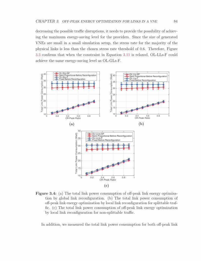
CHAPTER 3. OFF-PEAK ENERGY OPTIMIZATION FOR LINKS IN A VNE 84
decreasing the possible traffic disruptions, it needs to provide the possibility of achiev-
ing the maximum energy-saving level for the providers. Since the size of generated
VNEs are small in a small simulation setup, the stress rate for the majority of the
physical links is less than the chosen stress rate threshold of 0.6. Therefore, Figure
3.3 confirms that when the constraint in Equation 3.11 is relaxed, OL-LLs-F could
achieve the same energy-saving level as OL-GLs-F.
Off-Peak Ratio0 0.2 0.4 0.6 0.8 1
Tot
al L
ink
Pow
er C
onsu
mpt
ion
(Wat
t)
10
15
20
25
30
35
40 OL-GLs-SPSemi Proportional-Before ReconfigurationOL-GLs-FFixed-Before Reconfiguration
(a)
Off-Peak Ratio0 0.2 0.4 0.6 0.8 1
Tot
al L
ink
Pow
er C
onsu
mpt
ion
(Wat
t)10
15
20
25
30
35
40 OL-LLs-SPSemi Proportional-Before ReconfigurationOL-LLs-FFixed-Before Reconfiguration
(b)
Off-Peak Ratio0 0.2 0.4 0.6 0.8 1
Tot
al L
ink
Pow
er C
onsu
mpt
ion
(Wat
t)
10
15
20
25
30
35
40OL-LLns-SPSemi Proportional-Before ReconfigurationOL-LLns-FFixed-Before Reconfiguration
(c)
Figure 3.4: (a) The total link power consumption of off-peak link energy optimiza-tion by global link reconfiguration. (b) The total link power consumption ofoff-peak link energy optimization by local link reconfiguration for splittable traf-fic. (c) The total link power consumption of off-peak link energy optimizationby local link reconfiguration for non-splittable traffic.
In addition, we measured the total link power consumption for both off-peak link

CHAPTER 3. OFF-PEAK ENERGY OPTIMIZATION FOR LINKS IN A VNE 85
energy optimization by global link reconfiguration and local link reconfiguration so-
lutions on a small random simulation setup. This measurement has been performed
according to both Fixed and Semi-Proportional link power models. The total link
power consumption has been measured for the off-peak ratio range of 0.1 to 0.9, be-
fore and after applying the proposed energy-saving solutions. According to [56] and
because the random physical links’ capacities are generated uniformly in the range
of 100-200Mbps, P b is 0.9Watt and Pm is 1.0Watt for any physical link. The mea-
surement results for off-peak link energy optimization by global link reconfiguration,
and off-peak link energy optimization by local link reconfiguration for splittable and
non-splittable traffic, are shown in Figures 3.4a, 3.4b, and 3.4c, respectively.
The results in Figures 3.4a, 3.4b, and 3.4c, demonstrate that all of the formulated
programs are able to reduce a VNE’s link power consumption, effectively. Considering
the results of when Fixed link power model is used, the total link power consumption
for any off-peak traffic rate is constant, when no energy-saving solution is employed.
Nevertheless, the power consumption is changing with the traffic rate even before
applying any energy-saving solution, when Semi-Proportional link power model is
used. By applying any of the proposed energy-saving techniques (global/local link
reconfiguration), the total link power consumption based on both link power models
will be decreased. Note that increasing the off-peak ratio raises the total link power
consumption, as a larger number of links will be left activated.
In the same simulation setup, we calculated the percentage of power saved in
physical links, by the formulated programs for off-peak link energy optimization by
local link reconfiguration problem. This is tested in the case of splittable and non-
splittable traffic, for both Fixed and Semi-Proportional link power models. The results
are shown in Figure 3.5. The outcome of programs shows that the rate of power we
could save in physical links is decreasing when the off-peak ratio is increasing, because
the programs are more limited in terms of finding alternative paths.
Besides, Figure 3.5 illustrates that it is probable to save a higher amount of power
when traffic is splittable, in comparison to when traffic is non-splittable. This is
because the programs are more flexible in terms of finding alternative paths when
they could split the traffic to multiple paths. Moreover, Figure 3.5 confirms that we
could reach a higher rate of power-saving when the objective function is formulated
according to the Fixed link power model, in comparison to when the objective function
is formulated based on Semi-Proportional link power model. This is mainly due

CHAPTER 3. OFF-PEAK ENERGY OPTIMIZATION FOR LINKS IN A VNE 86
to two reasons. First, since the power consumption is varying based on the traffic
load in Semi-Proportional link power model rather than being a constant amount
based on Fixed link power model, a physical link’s power consumption in the case
of Semi-Proportional link power model is less than when Fixed link power model is
employed. Consequently, the amount of saved power with Semi-Proportional link
power model might be less than the amount of saved power with Fixed link power
model, if the program sets the same physical links into the sleep mode. In addition,
if the energy-saving program sets a physical link into the sleep mode, then it needs
to find an alternative path to support the off-peak traffic of the removed link. In the
case of Semi-Proportional link power model, the rerouted traffic increases the power
consumption over the alternative path. However, in the case of Fixed link power
model, since traffic load does not affect a link’s power consumption, the rerouted
traffic does not increase the power consumption over the alternative path.
Off-Peak Ratio0 0.2 0.4 0.6 0.8 1
Tot
al S
aved
Pow
er in
Phy
sica
l Lin
ks (
%)
20
25
30
35
40
45
50
55
60
65
70OL-LLs-SPOL-LLs-FOL-LLns-SPOL-LLns-F
Figure 3.5: The total saved power with off-peak link energy optimization by locallink reconfiguration for splittable and non-splittable traffic
3.5.2 The Heuristic
We solved the formulated BILP for OL-LLns-F and compared its ability in terms of
sleeping physical links to the proposed heuristic for the same problem. The average

CHAPTER 3. OFF-PEAK ENERGY OPTIMIZATION FOR LINKS IN A VNE 87
results are measured for the different off-peak traffic ratios on a small random sim-
ulation setup, and shown in Figure 3.6. The BILP results set the optimum points,
while the heuristic algorithm still reveals reasonable results. However, the heuristic
algorithm is considerably simpler and faster in terms of required run time.
It is also important to evaluate the effectiveness of the proposed heuristic algorithm
for OL-LLns-F. We assess the ability of the heuristic based on different factors on the
defined large random simulation setups.
Off-Peak Ratio0 0.2 0.4 0.6 0.8 1
Phy
sica
l Lin
ks in
Sle
ep M
odel
(%
)
0
10
20
30
40
50
60
70Heuristic for OL-LLns-FBILP for OL-LLns-F
Figure 3.6: The BILP vs. the heuristic for off-peak link energy optimization bylocal link reconfiguration (non-splittable traffic)
The heuristic is formulated based on Fixed link power model. In this regard, the
total link power consumption is measured for the different off-peak ratios, before and
after applying the proposed heuristic on a large random simulation setup. The average
results are shown in Figure 3.7. The power consumption is constant before applying
the heuristic. By applying the heuristic, the total VNE’s link power consumption
will be reduced. Note that increasing the off-peak ratio raises the total link power
consumption, as a larger number of links are left active.

CHAPTER 3. OFF-PEAK ENERGY OPTIMIZATION FOR LINKS IN A VNE 88
Off-Peak Ratio0 0.2 0.4 0.6 0.8 1
Tot
al L
ink
Pow
er C
onsu
mpt
ion
(Wat
t)
0
100
200
300
400
500
600
After ReconfigurationBefore Reconfiguration
Figure 3.7: The total link power consumption of the heuristic for off-peak linkenergy optimization by local link reconfiguration
Besides, it is essential to check the ability of the heuristic for different numbers of
involved virtual networks, as increasing the number of virtual networks adds several
constraints in terms of sleeping a single physical link. The ability of the proposed
heuristic on setting physical links into the sleep mode during the off-peak hours, is
tested over two large random simulation setups. In the first large random setup, each
VNE contains two virtual networks, but in the second large random setup, every VNE
includes three virtual networks. The effectiveness of the algorithm is evaluated for
the range of off-peak traffic ratios. The average results for both setups are shown in
Figure 3.8. Figure 3.8 shows that it is probable to set a notable number of physical
links into the sleep mode during the off-peak period, by implementing the suggested
heuristic algorithm. For the first setup, when the off-peak traffic ratio is 0.1, the
proposed heuristic sets 89.1230% of the physical links into the sleep mode. This
happens while the reconfiguration heuristic still accommodates the off-peak traffic
demands of involved VNs. In addition, Figure 3.8 confirms that mapping an extra
virtual network onto the substrate network degrades the ability of heuristic in terms
of saving power. This is because the algorithm assesses the allocated traffic capacities
to every virtual link in each substrate link in order to find a replaced path. By adding
new virtual networks, new virtual links are mapped onto physical links, and therefore

CHAPTER 3. OFF-PEAK ENERGY OPTIMIZATION FOR LINKS IN A VNE 89
there are more constraints for the algorithm. Consequently, a smaller number of
physical links is capable to be set into the sleep mode over off-peak hours. Moreover,
decreasing the off-peak ratio decreases the difference between outcome of the first and
second simulation setups. When off-peak traffic rate is low, the programs are more
flexible in terms of finding alternative paths. Hence, the energy-saving ability of the
programs is less affected by adding extra virtual networks when the off-peak ratio is
small, in comparison to when we have large off-peak traffic rates.
Off-Peak Ratio0 0.2 0.4 0.6 0.8 1
Phy
sica
l Lin
ks in
Sle
ep M
ode
(%)
72
74
76
78
80
82
84
86
88
90Each scenario has 2 VNsEach scneario has 3 VNs
Figure 3.8: The link reconfiguration heuristic for the different numbers of involvedVNs
Moreover, it is explained in Section 3.4 that the proposed heuristic, similar to the
formulated BILP for OL-LLns-F, does not re-allocate the allocated traffic capacities
in physical links with s(li,js ) ≥ T , in order to decrease the service disruptions due to
the reconfiguration. Figure 3.9 studies the effect of changing the stress rate threshold
T on the capability of the heuristic for setting physical links into the sleep mode,
over a large random simulation setup. Figure 3.9 shows that decreasing T , decreases
the number of physical links the heuristic sets into the sleep mode, because a smaller
number of substrate links are considered for energy-saving. Although setting a smaller
T decreases the amount of power the solutions could save, it reduces the traffic
interruptions, due to the reconfiguration. Consequently, the providers could control
the possible traffic interruptions by adjusting T . Note that because of the specific

CHAPTER 3. OFF-PEAK ENERGY OPTIMIZATION FOR LINKS IN A VNE 90
chosen amounts of physical and virtual links’ bandwidth capacity in our defined large
random simulation setups, the stress rate of the majority of the physical links in the
considered simulation setup is less than 0.3. Consequently, the heuristic outcome is
almost constant for T of greater than 0.3.
Stress Rate Threshold0 0.2 0.4 0.6 0.8 1
Phy
sica
l Lin
ks in
Sle
ep M
ode
(%)
78
78.5
79
79.5
80
80.5
81
81.5
82
82.5
83
Figure 3.9: The effect of changing the stress rate threshold on the heuristic’s out-come
Additionally, the suggested heuristic for OL-LLns-SP is expected to be more ef-
fective in comparison to our previous work [70] and other similar studies in [76, 77].
We compared the outcome of the proposed heuristic in this chapter to our previous
algorithm in [70], over a large random simulation setup. As the result is clear in Fig-
ure 3.10, this link reconfiguration algorithm is able to set a larger number of physical
links into the sleep mode over the off-peak time, with the same constraints. This is
because the methods in [70, 76, 77] do not modify the allocation of mapped virtual
networks, while they only reroute the traffic to the already allocated traffic capacities
to virtual links. Nonetheless, in this chapter, we reconfigure the mapping of virtual
links to reach higher power-saving rates.

CHAPTER 3. OFF-PEAK ENERGY OPTIMIZATION FOR LINKS IN A VNE 91
Off-Peak Ratio0 0.2 0.4 0.6 0.8 1
Phy
sica
l Lin
ks in
Sle
ep M
ode
(%)
0
10
20
30
40
50
60
70
80
90
100Our Previous AlgorithmReconfiguration Heuristic
Figure 3.10: The link reconfiguration heuristic vs. our previous algorithm
Off-Peak Ratio0.1 0.2 0.3 0.4 0.5 0.6 0.7 0.8 0.9
Mea
n U
tiliz
atio
n
0
0.2
0.4
0.6
0.8
1Peak TimeOff-Peak Time before ReconfigurationOff-Peak Time after Reconfiguration
Figure 3.11: The mean link utilization over different configurations
Furthermore, re-allocating the traffic capacities in the other substate links causes
changes to the link utilization. Accordingly, it is needed to make sure the increased
utilization is controlled and does not cause congestion. The link utilization for three
different configurations is tested on a large random simulation setup, and the average
results are shown in Figure 3.11. The first configuration is for the peak time when
allocated bandwidth is able to handle “Worst-Case” scenarios. The second configura-
tion is for the off-peak period while no energy-saving algorithm is implemented. Over

CHAPTER 3. OFF-PEAK ENERGY OPTIMIZATION FOR LINKS IN A VNE 92
this period the links are less utilized while the same bandwidth capacity is allocated
and consume the same power as the peak time. After applying our suggested heuris-
tic, the average link utilization is increased, but it is still less than the maximum
utilization. Note that the link utilization shown in Figure 3.11 is the mean of the
maximum points of all the test scenarios.
It is also necessary to validate the effectiveness of our proposed approach against
a real topology. In this regard, we tested the proposed heuristic on a new random
simulation setup that contains 10 randomly generated VNEs. Each VNE in this new
random simulation setup, has 2 random virtual networks that are mapped onto the
GEANT network topology [89], while every virtual network has 10 nodes. GEANT
has 22 nodes and 36 bidirectional links. We considered GEANT network as the
substrate network, because it is a real universal topology. Figure 3.12 shows the
results for this setup. The results confirm that the heuristic is able to effectively
reduce the network’s link power consumption.
Off-Peak Ratio0 0.2 0.4 0.6 0.8 1
Tot
al L
ink
Pow
er C
onsu
mpt
ion
(Wat
t)
20
30
40
50
60
70
80 Before ReconfigurationAfter Reconfiguration
Figure 3.12: The total link power consumption before and after applying the heuris-tic on the GEANT simulation setup
All the formulated ILPs in this chapter are NP-hard, while the complexity of
the proposed heuristic algorithm is O (|Es|3|Φ|2|Emv |2(|Es|+ |Vs|log|Vs|)). So, it is
expected the proposed heuristic needs less run time in comparison to the formulated
integer linear programs. We verified run time for each method (when the objective

CHAPTER 3. OFF-PEAK ENERGY OPTIMIZATION FOR LINKS IN A VNE 93
is defined based on Fixed link power model) on a single small random VNE that
has a substrate network and 2 virtual networks, while each has 10 nodes. The run
time is measured for each formulated optimization program as well as the heuristic,
when the off-peak ratio is 0.5. The results are shown in Figure 3.13. The run time
of the MILPs for OL-GLs-F and OL-LLs-F are 215.7 seconds and 3,302.4 seconds,
respectively. Besides, the run time of the BILP for OL-LLns-F is 20,322.0 seconds.
However, the run time of the heuristic for OL-LLns-F is only 0.0409 seconds, which
is considerably small in comparison to the required run time for the formulated BILP
of the same problem. The run time for local link reconfiguration BILP for non-
splittable traffic is higher than the MILP of the same problem for splittable traffic.
This is because the BILP needs to find an alternative path for every allocated traffic
capacity in substrate links, while the MILP has to find an alternative path for every
bundled traffic capacity. Therefore, the BILP for non-splittable traffic has more
constraints than the MILP for splittable traffic. In addition, the run time of local
link reconfiguration MILP for splittable traffic is larger than the run time for global
link reconfiguration MILP, since the local link reconfiguration is more complex and
has a larger number of constraints than the global link reconfiguration.
0
0.5
1
1.5
2
2.5x 10
4
Run
TIm
e (S
ec)
BILPfor
OL−LLns−F
20322
0.0409
Heuristicfor
OL−LLns−F215.7733
3302.4
MILPfor
OL−LLs−FMILPfor
OL−GLs−F
Figure 3.13: The run time for different methods
The simulation results prove the suggested energy-saving solutions are able to
reduce a VNE’s link power consumption, during the off-peak period, effectively. Be-
sides, the proposed heuristic is a simple and fast algorithm that works closely to the

CHAPTER 3. OFF-PEAK ENERGY OPTIMIZATION FOR LINKS IN A VNE 94
optimum points. Note that every simulation setup is quite large to cover a substan-
tial number of random topologies in order to verify the effectiveness of the proposed
solutions. Besides, the calculated confidence intervals confirm that the results are
precise enough to reveal significances of suggested energy-saving methods.
3.6 Summary
In this chapter, we discussed multiple novel energy-saving solutions that glob-
ally/locally optimize a VNE’s link energy consumption, during the off-peak time.
The proposed fine-grained local reconfiguration enables the providers to adjust the
level of the reconfiguration, and accordingly control the possible traffic disruptions.
An Integer Linear Program (ILP) is formulated for each problem. Since the ILPs are
NP-hard, a novel heuristic algorithm is also proposed. Simulation results show that
the energy-saving solutions are noticeably effective and the heuristic achieves closely
to the optimum points. Because physical nodes are also essential energy consumers in
VNEs, it is necessary to develop energy-saving techniques that minimize both node
and link energy consumption in a VNE. This will be discussed in the next chapter.

Chapter 4
Off-Peak Energy Optimization for Nodes
and Links in a VNE
4.1 Introduction
In Chapter 3 we studied multiple energy-saving solutions for the off-peak period of
a VNE. The provided solutions are developed to reduce only a VNE’s link energy
consumption. However, physical nodes are also essential energy consumers in VNEs.
According to the discussed power models in Section 2.3, physical nodes normally con-
sume larger amounts of power than physical links. Consequently, it is necessary to
develop energy-saving techniques that optimize both node and link energy consump-
tion in a VNE.
In this chapter, we extend our previous study in Chapter 3, and discuss multiple
novel energy-saving solutions that optimize a VNE’s node and link energy consump-
tion during the off-peak time, according to two defined power models. We approach
the problem by reconfiguring the mapping for some of the already embedded virtual
nodes and links. We assume that substrate and virtual networks are homogeneous.
All the substrate and virtual nodes are assumed to be switches/routers to reflect the
network environment. This is the case in the majority of existing related research
studies.
In this regard, first, we formulated a Mixed Integer Linear Program (MILP) for
off-peak node and link energy optimization by local node and link reconfiguration.
A stress rate is defined for substrate nodes. Accordingly, the MILP may set less
stressed substrate nodes and their adjacent substrate links into the sleep mode for
the off-peak time. We re-map a virtual link if and only if we sleep the substrate node
95

CHAPTER 4. OFF-PEAK ENERGY OPTIMIZATION FOR NODE AND LINKS IN A VNE 96
that hosts its source/sink virtual node, or at least one substrate node that relays its
traffic over its embedded path. The energy consumption of a re-mapped virtual link
is also minimized.
Because reconfiguring the mapping for both of virtual nodes and virtual links may
be expensive and cause the interruptions to the normal network operations, we come
up with another methodology that optimizes node and link energy consumption of a
VNE, during the off-peak time, by reconfiguring the mapping for only some of the
virtual links. We do not reconfigure the mapping of the embedded virtual nodes in
this case. We call the latter problem off-peak node and link energy optimization by
local link reconfiguration. We define a different stress rate for intermediate substrate
nodes, which do not host a virtual node and only relay the traffic. Accordingly, a
solution is proposed to optimize the total energy consumption of the intermediate
substrate nodes and substrate links during the off-peak time. This method might
set the less stressed intermediate substrate nodes and their respective substrate links
into the sleep mode for the off-peak time. We re-map a virtual link if and only if we
sleep at least one intermediate substrate node over its embedded path. The energy
consumption of a re-mapped virtual link is also minimized. An MILP for splittable
traffic and a Binary Integer Linear Program (BILP) for non-splittable traffic are
formulated for this strategy.
These methods enable the providers to change the level of the reconfiguration
by adjusting the stress rate’s threshold. Therefore, they can control the possible
traffic interruptions of the reconfiguration. Clearly, there is a trade-off between the
energy-saving level and the possible traffic interruptions.
Since the formulated optimization programs are NP-hard, we also suggest a
heuristic algorithm for off-peak node and link energy optimization by local link recon-
figuration. The simulation results confirm that the heuristic algorithm can achieve
closely to the optimum points set by the formulated optimization program, while it
is considerably faster. The proposed heuristic is scalable to large network sizes.
The related works are discussed in Section 2.3.3. In this regard, our contributions
in this chapter are:
• We propose a local optimization program in the form of an MILP that recon-
figures the mapping of both virtual nodes and links during the off-peak time,
to minimize the total energy consumption of nodes and links in a VNE in that
period.

CHAPTER 4. OFF-PEAK ENERGY OPTIMIZATION FOR NODE AND LINKS IN A VNE 97
• We propose local optimization programs in form of ILPs that reconfigure the
mapping of virtual links during the off-peak time, to minimize the energy con-
sumption of intermediate nodes and links in a VNE in that period.
• The solutions are formulated according to two power models.
• Different programs are formulated for splittable and non-splittable traffic in
order to study the impact of traffic splittablity.
• We present a scalable heuristic algorithm that can achieve closely to the opti-
mum results, but considerably faster than the optimization program.
• We define different stress rates for distinct types of substrate nodes. Therefore,
different from any related research studies, the proposed methods enable the
providers to control the level of reconfiguration and the possible traffic inter-
ruptions.
• Different from previous research studies [17,60,62,64,69], our method does not
decrease the network admittance ratio for new virtual networks. This is because
we reconfigure the mapping of the already accepted VNs only for the off-peak
period, and they could be reconfigured back to their peak the mapping in the
case of an unexpected new demand.
• Our solutions are not limited to a sub-topology as the case in [70], and so they
have a larger degree of freedom to save the energy.
• We do not move VMs, so our method does not have the difficulties of [16].
• We assess the impact of different parameters on the energy-saving capability of
the discussed solutions, through extensive simulations.
• To the best of our knowledge, these problems are not defined and formulated
mathematically in any published study.
This chapter is organized as follows: Two power models for physical nodes and
links are reviewed in Section 4.2. Multiple optimization programs are defined and
formulated as ILPs in Section 4.3 and the suggested heuristic is discussed in Section
4.4. In order to evaluate the performance of the ILPs as well as the heuristic algorithm,
multiple random scenarios have been simulated over randomly generated VNEs and
the results are analyzed in Section 4.5. The chapter will conclude in Section 4.6.

CHAPTER 4. OFF-PEAK ENERGY OPTIMIZATION FOR NODE AND LINKS IN A VNE 98
4.2 Power Models
Various node and link power models are reviewed in Sections 2.3.1 and 2.3.2, respec-
tively. In this chapter, we assume that substrate networks are homogeneous. All
the substrate nodes are assumed to be switches/routers to reflect the network envi-
ronment. Note that the proposed solutions are general, and they could also employ
physical server power models. We discuss our energy-saving solutions according to
Fixed power model and Semi-Proportional power model.
Equation 2.45 defines the actual power consumption p(vis) for a physical node vis,
based on Fixed power model. The actual power consumption p(li,js ) of a physical link
li,js can be found by Equation 2.58, according to Fixed power model.
In addition, Equation 2.46 defines the actual power consumption p(vis) of a sub-
strate node vis according to Semi-Proportional power model. Similar to the node power
model, Equation 2.59 defines the actual power consumption p(li,js ) of a physical link
li,js based on Semi-Proportional power model.
Because switches/routers are considered as the physical nodes, pb(vis) and pm(vis)
can be determined by Equation 4.1 and Equation 4.2, respectively [56,57]. pb(vis) and
pm(vis) for a server physical node could be found through calibration experiments as
described in [59].
pb(vis) = 0.85Cb(vis)
23 (4.1)
pm(vis) = Cb(vis)
23 (4.2)
Consequently, p(vis) for the case of Semi-Proportional power model could be re-
written as Equation 4.3.
p(vis) = 0.85α(vis)Cb(vis)
23 +
0.15r(vis)
Cb(vis)13
(4.3)
In addition, pb(li,js ) and pm(li,js ) for a physical link are depended to the physical
link bandwidth capacity Cb(li,js ), its length, and the cable type.
Today’s networks are designed based on Fixed power model, so it is a common
model that is widely used [56]. Nevertheless, it is not efficient that an active physical
node or link consumes a constant amount of power, regardless of its traffic load.
Therefore, the physical nodes and links are expected to get modified, so their power

CHAPTER 4. OFF-PEAK ENERGY OPTIMIZATION FOR NODE AND LINKS IN A VNE 99
consumption will be more adaptive to their traffic load. The Semi-Proportional power
model brings a traffic-adaptive power model that formulates the power consumption
of a physical node or link according to its traffic load.
A power model determines the energy-saving methodology. In this chapter, we
assume all the substrate links are in the same range of bandwidth capacity, so they
consume the same amount of power. First, considering Fixed power model, a physical
node or link consumes a constant amount of power, regardless of the traffic load.
Therefore, the best energy-saving strategy to minimize a physical node or link’s energy
consumption is setting the device into the sleep mode. However, because physical
nodes consume considerably a larger amount of power in comparison to physical
links, it is more important to set a physical node into the sleep mode, rather than a
physical link. Second, in the case of Semi-Proportional power model, the traffic load
in a device changes its power consumption. Although a large portion of power is still
consumed to keep the device operational, it might be possible to save some energy by
rerouting the device’s traffic to other active nodes and links with the larger value for
the division of the difference between the maximum and the base power consumption
by the bandwidth capacity. So, in the case of Semi-Proportional power model it
may be feasible to save energy by sleeping a network element, or rerouting the traffic.
Consequently, the objective for an energy-saving solution based on Fixed power model
is different to the objective for an energy-saving method based on Semi-Proportional
power model. In this regard, we formulate multiple node and link energy-saving
solutions according to the both power models.
4.3 Integer Linear Programs
During the off-peak time of a VNE, the virtual networks’ demands in terms of traffic,
processing, etc., are decreased. Accordingly, it might be achievable to save notable
amounts of energy in substrate nodes and links, by reconfiguring the mapping of the
already allocated resources, while still satisfying the off-peak demands. In this regard,
we define a general reconfiguration problem that targets mapping of both physical
nodes and links to minimize a VNE’s energy consumption during the off-peak period.
The problem description is the followings:
Given:
• A homogeneous substrate network topology

CHAPTER 4. OFF-PEAK ENERGY OPTIMIZATION FOR NODE AND LINKS IN A VNE 100
• Allocated virtual networks’ topologies
• For each substrate node: The physical bandwidth capacity, and the processing
capacity, as well as the allocated processing capacity to each virtual node in the
substrate node
• For each substrate link: The physical bandwidth capacity, as well as the allo-
cated bandwidth capacity to every virtual link in the substrate link
• Off-peak traffic and processing demands of each virtual network, provided by
virtual network customers, or network traffic prediction techniques
Find:
• The modified off-peak VNE mapping that leads to the minimum total node and
link energy consumption during the off-peak time
Constraints:
• Supporting the off-peak traffic and processing demands
We approach the defined energy-saving problem with two different local reconfigu-
ration strategies. First, we reconfigure the mapping for some of the already allocated
virtual nodes and links, during the off-peak period, to minimize the total node and
link energy consumption of the network in that period. It is possible to minimize a
VNE’s total energy consumption by setting any capable physical node or link into the
sleep mode, or rerouting its traffic load. Rerouting the traffic may also help saving
the energy. However, we still need to accommodate the demanded off-peak processing
and traffic rates. We call this problem off-peak node and link energy optimization by
local node and link reconfiguration.
Reconfiguring the mapping for both of virtual nodes and links might be expensive
or cause the interruptions to the normal network operations. Besides, some times it
is infeasible to reconfigure the mapping of virtual nodes. For example, moving an
embedded access/edge virtual node to the other part of a substrate network might
be impossible. An access/edge virtual node connects a VN to other networks (on
different substrate networks). Hence, we come up with the second reconfiguration
method that optimizes total node and link energy consumption in a VNE during the
off-peak time, by reconfiguring the mapping for only some of the already allocated

CHAPTER 4. OFF-PEAK ENERGY OPTIMIZATION FOR NODE AND LINKS IN A VNE 101
virtual links. The second method does not reconfigure the already allocated virtual
nodes, and therefore it is not possible to sleep the physical nodes that one or multiple
virtual nodes are allocated in them. However, it is probable to save the energy in
the capable intermediate substrate nodes, or any qualified substrate link. Rerouting
traffic load over the network may also help to save energy based on some power
models. We call the second problem off-peak node and link energy optimization by
local link reconfiguration.
Both of the reconfiguration strategies are local optimization problems, as they
do not reconfigure the mapping for all of the virtual nodes or links. This helps
to reduce the possible interruptions to the network operations. Although the second
reconfiguration strategy does not reconfigure virtual nodes and therefore it is expected
to save smaller amounts of energy in comparison to the first method, it causes fewer
interruptions to the normal network operations.
Note that virtual network customers might have multiple constraints for their
demanded virtual nodes and links. In this chapter, we concern only with the requested
switching and processing capacity for switches/routers, and the traffic demands.
In this regard, first, we model a VNE mathematically. Afterwards, for both Fixed
and Semi-Proportional power models, we formulate integer linear programs for off-
peak node and link energy optimization by local node and link reconfiguration, and
off-peak node and link energy optimization by local link reconfiguration. Since the
traffic type (splittable/non-splittable) has a major impact on the solution’s method-
ology, we formulate off-peak node and link energy optimization by local link recon-
figuration for both splittable and non-splittable traffic.
4.3.1 The Network Model
A substrate network is modeled similar to the substrate network model in Section
3.3.1. Cc(vis) expresses the processing capacity of vis.
The nth virtual network is also modeled similar to Section 3.3.1. In addition, vkn
refers to the kth virtual node in the nth virtual network. Cc(vkn) represents off-peak
processing demand of vkn.
In a VNE embedding procedure, the nth requested virtual network Gn is mapped
onto a defined substrate network Gs: Gn → Gs. Virtual nodes are allocated in the
chosen physical nodes. φ(vkn, vis) indicates whether a virtual node vkn is allocated in
a physical node vis, or not. φ(vkn, vis) is 1, if v
kn is allocated in vis. Otherwise, it is 0.

CHAPTER 4. OFF-PEAK ENERGY OPTIMIZATION FOR NODE AND LINKS IN A VNE 102
A virtual link could be mapped onto a single physical link, or multiple physical links
that makes a physical path. If traffic is splittable, then a virtual link could be mapped
onto multiple substrate paths. However, if traffic is non-splittable, then each traffic
demand is carried by only one path. The allocated virtual links of the nth VN are
presented as the set of ordered allocated virtual node pairs (am, bm), m = 1, 2, . . . , Ln.
lam,bmn represents the mth virtual link, belonging to the nth VN, that connects the
virtual node mapped onto the amth substrate node to the virtual node mapped onto
the bmth substrate node. rmn stands for the off-peak traffic demand of lam,bmn . In
addition, ri,jn (m) denotes the off-peak traffic demand of the allocated traffic capacity
to lam,bmn in li,js . During the off-peak period, the reserved processing and traffic capacity
for virtual nodes and links in physical nodes and links, respectively, are equal to their
particular off-peak demands, and the rest of the physical capacity could be shared.
4.3.2 Programs Based on Fixed Power Model
In this section, we develop the energy-saving solutions based on Fixed power model.
It is assumed that all the substrate links are in the same range of the bandwidth
capacity. Conforming to Fixed power model, the best energy-saving strategy to reduce
a physical node or link’s energy consumption is setting the device into the sleep mode.
The following energy-saving methods are formulated according to this logic.
Off-peak Node and Link Energy Optimization by Local Node and Link
Reconfiguration (ONL-LNLs-F)
We define a stress rate for a substrate node. Accordingly, an MILP is formulated
for the problem. The MILP may set less stressed substrate nodes and their adjacent
substrate links into the sleep mode for the off-peak time. We re-map a virtual link if
and only if we sleep the substrate node that hosts its source/sink virtual node, or at
least one substrate node that relay its traffic over its embedded path. The program
also sets the maximum number of physical links into the sleep mode during the re-
allocation process of virtual links. This problem is defined according to Fixed power
model. The traffic is assumed to be splittable in this problem to deliver the highest
level of energy-saving. We call this problem ONL-LNLs-F.
In this problem, the stress rate s1(vis) of a physical node vis reveals the intensity
of total off-peak processing and traffic demands in the node. Equation 4.4 defines
s1(vis).

CHAPTER 4. OFF-PEAK ENERGY OPTIMIZATION FOR NODE AND LINKS IN A VNE 103
s1(vis) =
∑{n|Gn∈Φ}
∑k∈Vn
φ(vkn, vis)Cc(v
kn)
Cc(vis)
(∑{j|(i,j)∈Es}
∑{n|Gn∈Φ}
∑Ln
m=1 ri,jn (m)
Cb(vis)
+
∑{j|(j,i)∈Es}
∑{n|Gn∈Φ}
∑Ln
m=1 rj,in (m)
Cb(vis)
)(4.4)
s1(vis) considers two parameters. The first parameter is the fraction of the total
off-peak processing demands of allocated virtual nodes in a physical node, over the
processing capacity of the physical node. The second parameter considers the off-
peak traffic by finding the fraction of the total off-peak traffic passing a physical
node, over the physical bandwidth capacity of the node. Note that, in this chapter,
we assume that the total traffic in a substrate node is the total traffic in its incoming
physical links plus the total traffic in its outgoing physical links. This also defines
the switching capacity of a substrate node. Accordingly, s1(vis) considers the off-
peak traffic intensity by considering both incoming and outgoing off-peak traffic to a
substrate node. However, if a node is the source/sink of traffic, then it considers only
one of the the flows, as the other one is zero.
Consequently, in this problem, a higher physical node’s stress rate means the node
is more utilized in terms of off-peak processing and traffic demands. In this regard, we
do not re-map a virtual node that is mapped onto a physical node with s1(vis) ≥ T ,
in order to decrease the traffic disruptions due to the reconfiguration. T is the stress
rate’s threshold, and it is a real number between 0 and 1. The providers can adjust T .
Decreasing the value of T degrades the amount of energy the programs could save,
but also reduces the traffic interruptions due to the reconfiguration. This is because
a smaller number of physical nodes and links are considered for energy-saving.
We formulate ONL-LNLs-F as an MILP. ONL-LNLs-F is a combination of two
sub-problems with the same objective. The first sub-problem is a node reconfiguration
problem that reconfigures the mapping of virtual nodes. The second sub-problem is a
link reconfiguration problem that reconfigures the mapping of virtual links. The link
reconfiguration sub-problem could be formulated as a multi-commodity flow problem.
In the context of this sub-problem, a virtual link is a commodity. Multiple virtual
links are multiple commodities. In order to achieve the most optimum result, it
is required to formulate a single problem that combines both of the sub-problems
together.

CHAPTER 4. OFF-PEAK ENERGY OPTIMIZATION FOR NODE AND LINKS IN A VNE 104
The substrate network is known to the program, and therefore the bandwidth
capacity of every physical node and link, as well as the processing capacity of each
physical node are given. The allocated virtual networks are also identified, so φ(vkn, vis)
for any virtual node in every physical node is specified. In addition, the off-peak
processing demand Cc(vkn) of every virtual node is known to the program. In the
context of link reconfiguration sub-problem, we have Ln commodities for the nth
virtual network. For each lam,bmn , as a commodity, we are given a scalar rmn that refers
to the virtual link’s off-peak traffic demand. Besides, ri,jn (m) for every virtual link in
each physical link is specified. Moreover, �′mn (vis) is 1, if v
is is a relay substrate node
for lam,bmn . vis is a relay node for lam,bm
n , if source or sink virtual node of lam,bmn is not
mapped onto vis, while vis is on the allocated path for lam,bmn and forwards its traffic.
Otherwise, �′mn (vis) is 0.
Therefore, ONL-LNLs-F is formulated as an MILP as follows:
Optimization Variables:
• α(vis) is a binary variable. It denotes the status of vis. α(vis) is 1 in the case vis
is active, otherwise it is 0.
• α(li,js ) is a binary variable. It refers to the status of li,js . α(li,js ) is 1 in the case
li,js is active, otherwise it is 0.
• φ(vkn, vis) is a binary variable that expresses whether a virtual node vkn is re-
allocated in a physical node vis, during the reconfiguration process, or not. If
the program re-allocates vkn in vis, then φ(vkn, vis) is 1. Otherwise, φ(vkn, v
is) is 0.
• f ′i,jn (m) is a real-valued variable. It denotes the re-allocated off-peak traffic
capacity to the mth virtual link of the nth virtual network, in li,js . f ′i,jn (m) is
the result of the node reconfiguration sub-problem.
• ωmn is a binary variable. It is 1, if the program sets at least a relay node for
lam,bmn into the sleep mode. Otherwise, it is 0.
• ωmn is a binary variable. It is 1, if the program re-allocates the source virtual
node vamn , or the sink virtual node vbmn of lam,bmn , or both of them to another
physical node. Otherwise, it is 0.

CHAPTER 4. OFF-PEAK ENERGY OPTIMIZATION FOR NODE AND LINKS IN A VNE 105
• f i,jn (m) is a real-valued variable. It denotes the re-allocated off-peak traffic
capacity to the mth virtual link of the nth virtual network, in li,js . f i,jn (m) is
the result of link reconfiguration sub-problem.
Objective Function: This program intends to minimize VNE’s total node and link en-
ergy consumption, during the off-peak time, according to Fixed power model. Equa-
tion 4.5 maintains this objective.
Minimize
⎧⎨⎩∑
i∈Vs
α(vis)pm(vis) +
∑(i,j)∈Es
α(li,js )pm(li,js )
⎫⎬⎭ (4.5)
Constraints: A substrate node might host virtual nodes, and may also relay the traffic
of other virtual nodes. In this regard, setting a substrate node into the sleep mode
requires satisfying some constraints to maintain virtual networks’ off-peak processing
and traffic demands. In regard to the node reconfiguration sub-problem, if the pro-
gram decides to set a physical node vis into the sleep mode, then it needs to suggest
an alternative physical node for each of the allocated virtual nodes in vis. Equation
4.6 preserves this condition. If vkn is already allocated in vis, then φ(vkn, vis) is 1. In the
case the program sets vis into the sleep mode, α(vis) is 0. Therefore,∑
j∈Vsφ(vkn, v
js)
must be 1, which means vkn is re-allocated in an alternative physical node. This con-
straint also ensures the program re-allocates a virtual node only in a single alternative
physical node. However, if vkn is not allocated in vis, then φ(vkn, vis) is 0, and therefore
the constraint in Equation 4.6 is always satisfied. Note that if the program leaves vis
active, then none of the allocated virtual nodes in vis could be re-allocated.
φ(vkn, vis)
(1− α(vis)−
∑j∈Vs
φ(vkn, vjs)
)= 0 , ∀i ∈ Vs, ∀n ∈ {n|Gn ∈ Φ}, ∀k ∈ Vn
(4.6)
An alternative physical node needs to have some specifications. First, it has to support
the off-peak processing demand Cc(vkn) of v
kn. In this regard, as stated in the constraint
in Equation 4.7, the physical processing capacity Cc(vis) of every substrate node must
be equal or greater than the total off-peak processing rate of already allocated and
not re-mapped virtual nodes in the substrate node (∑
{n|Gn∈Φ}∑
k∈Vnφ(vkn, v
is)Cc(v
kn)),
plus the total off-peak processing demand of re-allocated virtual nodes in the substrate

CHAPTER 4. OFF-PEAK ENERGY OPTIMIZATION FOR NODE AND LINKS IN A VNE 106
node (∑
{n|Gn∈Φ}∑
k∈Vnφ(vkn, v
is)Cc(v
kn)).
∑{n|Gn∈Φ}
∑k∈Vn
φ(vkn, vis)Cc(v
kn)+
∑{n|Gn∈Φ}
∑k∈Vn
φ(vkn, vis)Cc(v
kn) ≤ Cc(v
is), ∀i ∈ Vs (4.7)
Second, the replaced physical node must be active. The constraint in Equation 4.8
retains this concern. If vis was set into the sleep mode, then α(vis) is 0, and therefore∑{n|Gn∈Φ}
∑k∈Vn
φ(vkn, vis) must be 0, which means no virtual node can be re-allocated
in vis. This constraint, together with the constraint in Equation 4.6, ensures a virtual
node could not be re-allocated in the original substrate node, which is the physical
node that the virtual node was previously allocated in. Note that B1, B2, B3, B4,
and B5 are integer numbers, while they must be large enough to be greater than the
left hand side of their respective equations.
∑{n|Gn∈Φ}
∑k∈Vn
φ(vkn, vis) ≤ B1α(v
is) , ∀i ∈ Vs (4.8)
Third, each virtual node is associated with one or multiple virtual links. Hence,
as indicated in the constraints presented in Equation 4.9, we do not re-allocate the
source virtual node vamn and the sink virtual node vbmn of the mth virtual link in a
single substrate node. This is the case in the majority of the available VNE embedding
methods.
φ(vamn , vis) + φ(vbmn , vis) ≤ 1 , (4.9)
φ(vamn , vis) + φ(vbmn , vis) ≤ 1 ,
φ(vamn , vis) + φ(vbmn , vis) ≤ 1 ,
∀i ∈ Vs, ∀n ∈ {n|Gn ∈ Φ},m = 1, 2, . . . , Ln
Fourth, it must be possible to re-map the off-peak traffic demand of all the virtual
links belonging to the re-allocated virtual nodes. In this regard, first, we find the off-
peak traffic demand between virtual nodes in every pair of modified substrate nodes
to consider the re-allocation of virtual nodes. Supposing a pair of substrate nodes
like vis and vjs, Table 4.1 summarizes the possible re-allocation combinations for the
source virtual node vamn and the sink virtual node vbmn of lam,bmn in these substrate
nodes.

CHAPTER 4. OFF-PEAK ENERGY OPTIMIZATION FOR NODE AND LINKS IN A VNE 107
Table 4.1: Re-allocation combinations for virtual nodes of lam,bmn , and the required
off-peak traffic to be rerouted
φ(vamn , vis) φ(vamn , vis) φ(vbmn , vjs) φ(vbmn , vjs) Off-peak traffic to be rerouted
0 1 0 1 rmn
0 1 1 0 rmn
1 0 0 1 rmn
0 1 0 0 0
1 0 1 0 0
1 0 0 0 0
0 0 0 1 0
0 0 1 0 0
0 0 0 0 0
Table 4.1 determines the amount of off-peak traffic demand that needs to be re-
allocated due to reconfiguring the mapping of virtual links between virtual nodes on
every pair of substrate nodes. For instance, the first row indicates the source virtual
node of lam,bmn is re-allocated in vis, and the sink virtual node of lam,bm
n is re-allocated
in vjs, so the off-peak traffic demand of rmn needs to be re-mapped from the virtual
node in vis to the virtual node in vjs. However, in the second row, the source virtual
node of lam,bmn is re-allocated in vis, while its sink virtual node is already mapped onto
vjs, and it is not modified. Therefore, the off-peak traffic demand of rmn needs to be
re-mapped from virtual node in vis to the virtual node in vjs. The program derives the
amount of off-peak traffic capacity that is required to be re-allocated between virtual
nodes in any pair of physical nodes, for every virtual link.
Note that when both of the source and sink virtual nodes of a virtual link are
re-allocated in other physical nodes (first row), the off-peak traffic demand should
be re-mapped only between the re-allocated source and sink virtual nodes. However,
according to Table 4.1, in this case, the off-peak traffic demand might also be re-
mapped between the original virtual node and the re-allocated virtual nodes (second,
or third row), which is not desirable.
In consequence, di,jn (m)rmn is the off-peak traffic demand of lam,bmn that needs to
be re-allocated from the virtual node in vis to the virtual node in vjs. di,jn (m) can be
derived as expressed in Equation 4.11.

CHAPTER 4. OFF-PEAK ENERGY OPTIMIZATION FOR NODE AND LINKS IN A VNE 108
Hence, by specifying the amount of every off-peak traffic demand that needs re-
mapping, the constraint in Equation 4.10 preserves one or multiple paths between the
reconfigured source and sink virtual nodes. The constraint in Equation 4.10 and the
objective function force the program to choose the path with the minimum number
of active physical links. In the case there is no path between the modified virtual
nodes, the program does not reconfigure the mapping of them.
∑{j|(i,j)∈Es}
f ′i,jn (m)−
∑{j|(j,i)∈Es}
f ′j,in (m) =
∑j∈Vs
di,jn (m)rmn −∑j∈Vs
dj,in (m)rmn ,
∀i ∈ Vs, ∀n ∈ {n|Gn ∈ Φ},m = 1, 2, . . . , Ln (4.10)
where:
di,jn (m) =
(1−
∑x∈Vs
∑y∈Vs
φ(vamn , vxs )φ(vbmn , vys )
)(φ(vamn , vis)φ(v
bmn , vjs)
+ φ(vbmn , vjs)φ(vamn , vis)
)+ φ(vamn , vis)φ(v
bmn , vjs) (4.11)
As it is discussed, a substrate node vis might also forward the traffic of other virtual
nodes and play the relay role. So, it is essential to re-map the virtual links that vis
relays their traffic, before setting vis into the sleep mode. This is the link reconfigu-
ration sub-problem. In this regard, if one or multiple relay substrate nodes for lam,bmn
are set into the sleep mode, then Equation 4.12 sets the binary variable ωmn to 1.
Otherwise, ωmn is set to 0. In addition, if the source or sink virtual nodes of lam,bm
n ,
or both of them are re-allocated, then Equation 4.13 sets the binary variable ωmn to
1. Otherwise, ωmn is 0. In this phase, we intend to re-map only the virtual links that
one or multiple of their relay nodes over their allocated paths are set into the sleep
mode, while their source and sink virtual nodes are not re-allocated. By finding the
value of ωmn and ωm
n for every virtual link, ωmn − ωm
n ωmn indicates whether the virtual
link is needed to be re-mapped (ωmn − ωm
n ωmn = 1), or not (ωm
n − ωmn ω
mn = 0). The
constraint in Equation 4.14 re-maps the off-peak traffic demand of virtual links that
one or multiple of their relay substrate nodes are set into the sleep mode, and their
source and sink virtual nodes are not re-allocated. Note that the constraint in Equa-
tion 4.10 re-maps a virtual link, as a part of node reconfiguration sub-problem, if its
source or sink virtual node, or both of them are re-allocated in other physical nodes.

CHAPTER 4. OFF-PEAK ENERGY OPTIMIZATION FOR NODE AND LINKS IN A VNE 109
Therefore, the program does not consider re-mapping of such a virtual link, again.
ωmn ≤
∑i∈Vs
�′mn (vis)(1− α(vis)
)≤ B2ω
mn , (4.12)
ωmn ≤
∑i∈Vs
(φ(vamn , vis) + φ(vbmn , vis)
)≤ B3ω
mn , (4.13)
∀n ∈ {n|Gn ∈ Φ},m = 1, 2, . . . , Ln
∑{j|(i,j)∈Es}
f i,jn (m)−
∑{j|(j,i)∈Es}
f j,in (m) =
⎧⎪⎪⎪⎪⎨⎪⎪⎪⎪⎩
(ωmn − ωm
n ωmn ) r
mn if i = am
(ωmn ω
mn − ωm
n ) rmn if i = bm
0 otherwise
,
∀i ∈ Vs, ∀n ∈ {n|Gn ∈ Φ},m = 1, 2, . . . , Ln (4.14)
Re-allocating virtual links by either the constraint in Equation 4.10 or the
constraint in Equation 4.14, also requires satisfying some other constraints.
First, the program ensures in the constraint in Equation 4.15 that no
rerouted traffic passes through the sleeping physical nodes. The constraint
in Equation 4.15 ensures total outgoing re-allocated off-peak traffic capacity∑{j|(i,j)∈Es}
∑{n|Gn∈Φ}
∑Ln
m=1
(f i,jn (m) + f ′i,j
n (m)), and the total incoming re-allocated
off-peak traffic capacity∑
{j|(j,i)∈Es}∑
{n|Gn∈Φ}∑Ln
m=1
(f j,in (m) + f ′j,i
n (m)), in a sleep-
ing physical node (α(vis) = 0) is 0.
∑{j|(i,j)∈Es}
∑{n|Gn∈Φ}
Ln∑m=1
(f i,jn (m) + f ′i,j
n (m))
+∑
{j|(j,i)∈Es}
∑{n|Gn∈Φ}
Ln∑m=1
(f j,in (m) + f ′j,i
n (m))≤ B4α(v
is) ,
∀i ∈ Vs (4.15)
Second, the total embedded off-peak traffic capacity in every substrate link must be
equal or less than its physical bandwidth capacity, as indicated in the constraint in
Equation 4.16. In this program, three types of traffic capacities form the total embed-
ded off-peak traffic capacity in a substrate link li,js . The first type is the off-peak traffic

CHAPTER 4. OFF-PEAK ENERGY OPTIMIZATION FOR NODE AND LINKS IN A VNE 110
capacity of the virtual links that are not re-allocated through the reconfiguration pro-
cess. In this regard, none of the relay substrate nodes in the already allocated paths
for the virtual link is set into the sleep mode, and therefore 1 − ωmn = 1. Moreover,
the source and sink virtual nodes of the virtual link are not re-allocated during the
reconfiguration process, so 1− ωmn = 1. Nonetheless, if the virtual link is re-allocated,
then this off-peak traffic is not considered. The second type is the re-allocated off-
peak traffic capacity f ′i,jn (m) to a virtual link in the substrate link, as the result of
node reconfiguration sub-problem. However, the third type is the re-allocated off-
peak traffic capacity f i,jn (m) to a virtual link in the substrate link, as the result of
link reconfiguration sub-problem. Equation 4.17 defines the total traffic in a substrate
link.
r(li,js ) ≤ Cb(li,js ) , ∀(i, j) ∈ Es (4.16)
where:
r(li,js ) =∑
{n|Gn∈Φ}
Ln∑m=1
((1 − ωm
n )(1 − ωmn )r
i,jn (m) + f ′i,j
n (m) + f i,jn (m)
)(4.17)
Third, the total embedded off-peak traffic capacity in every substrate node must be
equal or less than its physical bandwidth capacity, as indicated in Equation 4.18. Note
that the total traffic in a substrate node is the total traffic in its incoming physical
links plus the total traffic in its outgoing physical links. Equation 4.19 defines the
total traffic in a substrate node.
r(vis) ≤ Cb(vis) , ∀i ∈ Vs (4.18)
where:
r(vis) =∑
{j|(i,j)∈Es}r(li,js ) +
∑{j|(j,i)∈Es}
r(lj,is ) (4.19)
Furthermore, we do not re-allocate the allocated virtual nodes in high stressed sub-
strate nodes, and the virtual links that all the physical nodes along their allocated
paths are high stressed. The constraint in Equation 4.20 determines a physical node
vis with s1(vis) ≥ T , must stay active α(vis) = 1. Consequently, Equation 4.6 does
not let the program to re-allocate any allocated virtual node in the physical node vis.
Besides, Equation 4.12, and Equation 4.13 ensure a virtual link that all the physical

CHAPTER 4. OFF-PEAK ENERGY OPTIMIZATION FOR NODE AND LINKS IN A VNE 111
nodes along their allocated paths are high stressed is not re-allocated.
∀i ∈ {i|i ∈ Vs, s1(vis) ≥ T } : α(vis) = 1 (4.20)
The constraint in Equation 4.21 makes the program linear by setting the auxiliary
binary variable α(li,js ) to 1, if there is any traffic in li,js . Otherwise, α(li,js ) is 0.
r(li,js ) ≤ B5α(li,js ) , ∀(i, j) ∈ Es (4.21)
The variables also must be in the following bounds:
f i,jn (m) ≥ 0, f ′i,j
n (m) ≥ 0 , ∀(i, j) ∈ Es, ∀n ∈ {n|Gn ∈ Φ},m = 1, 2, . . . , Ln (4.22)
α(li,js ) ∈ {0, 1} , ∀(i, j) ∈ Es (4.23)
α(vis) ∈ {0, 1} , ∀i ∈ Vs (4.24)
φ(vkn, vis) ∈ {0, 1} , ∀i ∈ Vs, ∀n ∈ {n|Gn ∈ Φ}, ∀k ∈ Vn (4.25)
ωmn ∈ {0, 1}, ωm
n ∈ {0, 1} , ∀n ∈ {n|Gn ∈ Φ},m = 1, 2, . . . , Ln (4.26)
There are some constraints in the program that include a product of binary vari-
ables. This issue makes the program nonlinear. However, a product of two binary
variables can be replaced by one new binary variable, on which a number of con-
straints is imposed to the program [90], and therefore the program remains linear.
The extension to the products of more binary variables is straightforward. Consid-
ering the binary variables x1 and x2, their product x1x2 could be replaced by a new
binary variable y, while the following constraints force y to take the value of x1x2.
y ≤ x1 (4.27)
y ≤ x2 (4.28)
y ≥ x1 + x2 − 1 (4.29)
y ∈ {0, 1} (4.30)
As it is described, the formulated MILP for ONL-LNLs-F includes two sub-
problems. The link reconfiguration sub-problem could be reduced to the problem

CHAPTER 4. OFF-PEAK ENERGY OPTIMIZATION FOR NODE AND LINKS IN A VNE 112
discussed in [83] that is a simple two-commodity integer flow problem. It is proven
in [83] that this simple two-commodity integer flow problem is NP-hard. Hence, our
formulated MILP for off-peak node and link energy optimization by local node and
link reconfiguration is NP-hard.
Off-peak Node and Link Energy Optimization by Local Link Reconfigu-
ration
We define a different stress rate for an intermediate substrate node in this section.
Accordingly, a solution is proposed to optimize total energy consumption of the in-
termediate substrate nodes and substrate links during the off-peak time. We do not
re-map a virtual node in this problem. This method might set the less stressed in-
termediate substrate nodes and their respective substrate links into the sleep mode
for the off-peak time. We re-map a virtual link if and only if we sleep at least one
intermediate substrate node over its embedded path. The programs also concern with
a VNE’s link energy consumption, by setting the maximum number of physical links
into the sleep mode during the re-allocation of virtual links. An MILP for splittable
traffic and a BILP for non-splittable traffic are formulated for this strategy.
The stress rate s2(vis) of a physical node vis in this problem, indicates the intensity
of involved VNs and the total off-peak traffic demand in the substrate node. The
definition of a physical node’s stress rate in this problem is different to the definition
of a physical node’s stress rate in the previous problem, because we do not reconfigure
virtual nodes here. A VN is involved in a substrate node vis, if at least one of its virtual
nodes is mapped onto vis, or at least one of its mapped virtual links passes through
vis. Assume η(vis) as the number of virtual networks involved in a physical node vis,
the following equation defines s2(vis).
s2(vis) =
η(vis)
|Φ|(∑{j|(i,j)∈Es}
∑{n|Gn∈Φ}
∑Ln
m=1 ri,jn (m)
Cb(vis)
+
∑{j|(j,i)∈Es}
∑{n|Gn∈Φ}
∑Ln
m=1 rj,in (m)
Cb(vis)
)(4.31)
s2(vis) considers two parameters. The first parameter is the fraction of the number
of involved VNs in a node, over the total number of active VNs. This parameter de-
notes the intensity of involved VNs in a vis. However, the second parameter considers

CHAPTER 4. OFF-PEAK ENERGY OPTIMIZATION FOR NODE AND LINKS IN A VNE 113
the off-peak traffic demand by finding the fraction of total off-peak traffic passes a
substrate node, over the bandwidth capacity of the node. Consequently, in this prob-
lem, a higher physical node’s stress rate means a larger number of VNs is involved in
the node, while the substrate node is more utilized in terms of off-peak traffic. In this
regard, we do not set an intermediate physical node with s2(vis) ≥ T into the sleep
mode. Virtual links that the stress rate of all the physical nodes along their allocated
paths are equal or greater than T are also not re-mapped. These actions help to
decrease the traffic disruptions due to the reconfiguration. Note that the threshold
value of T is adjustable. The providers could adjust the value of T , and therefore
manage the level of the reconfiguration. Decreasing the value of s2 threshold degrades
the amount of energy the programs could save and reduces the possible traffic inter-
ruptions, because a smaller number of physical nodes and links will be considered
for energy-saving. The impact of different values for the stress rate threshold on the
energy-saving ability of the solutions is discussed in Section 4.5.
The traffic might be splittable or non-splittable. In the splittable case, a traffic
demand of each virtual link could be carried by one or multiple paths in a substrate
network. However, if the traffic is non-splittable, then each virtual link’s traffic de-
mand may be required to follow the same path through the network, rather than be
divided among multiple paths. It is expected to save higher amounts of energy when
traffic is splittable, because we are more flexible in terms of finding alternative paths.
This is a major restriction that has an important impact on the solution’s methodol-
ogy. In this regard, we formulate off-peak node and link energy optimization by local
link reconfiguration for both splittable and non-splittable traffic.
Splittable Traffic (ONL-LLs-F) The defined local link reconfiguration problem,
in the case of splittable traffic, can be formulated as an MILP, in the category of
multi-commodity flow problems. In the context of this problem, every virtual link is
a commodity. The off-peak node and link energy optimization by local link reconfig-
uration that is formulated based on Fixed power model, when traffic is splittable, is
called ONL-LLs-F.
Similar to the previous problem, the substrate network topology is specified. The
physical bandwidth capacity of every substrate node and link is known. Allocated
virtual networks are also identified. In this problem, we have Ln commodities for the
nth virtual network. For each virtual link lam,bmn , as a commodity, we are given a

CHAPTER 4. OFF-PEAK ENERGY OPTIMIZATION FOR NODE AND LINKS IN A VNE 114
scalar rmn that refers to the virtual link’s off-peak traffic demand. ri,jn (m) for every
virtual link in each physical link is also known. Besides, �mn (vis) indicates whether
the allocated path for lam,bmn includes vis, or not. �
mn (v
is) is 1, if the allocated path for
lam,bmn contains vis. Otherwise, �mn (v
is) is 0.
Therefore, ONL-LLs-F is formulated as an MILP as follows:
Optimization Variables:
• α(vis) is a binary variable. It denotes the status of vis. α(vis) is 1 in the case vis
is active, otherwise it is 0.
• α(li,js ) is a binary variable. It refers to the status of li,js . α(li,js ) is 1 in the case
li,js is active, otherwise it is 0.
• ωmn is a binary variable. It is 1 in the case at least one physical node over the
allocated path for lam,bmn is set into the sleep mode. Otherwise, it is 0.
• f i,jn (m) is a real-valued variable. It denotes the re-allocated off-peak traffic
capacity to the mth virtual link of the nth virtual network, in li,js .
Objective Function: This program aims to minimize the total energy consumption by
physical intermediate nodes and physical links during the off-peak time, according
to Fixed power model. Equation 4.32, and the constraint in Equation 4.34 that
allows only intermediate substrate nodes to be set into the sleep mode, preserve this
objective.
Minimize
⎧⎨⎩∑
i∈Vs
α(vis)pm(vis) +
∑(i,j)∈Es
α(li,js )pm(li,js )
⎫⎬⎭ (4.32)
Constraints: If the program puts an intermediate physical node into the sleep mode,
then it needs to suggest one or more alternative paths for every virtual link that was
passing the substrate node. In this regard, the constraint in Equation 4.33 sets the
binary variable ωmn to 1, if at least one physical node vis, that is on the allocated path
for lam,bmn (�mn (v
is) = 1), is set into the sleep mode (α(vis) = 0). Otherwise, ωm
n is 0.
The program derives the ωmn for every virtual link. ωm
n determines whether lam,bmn is
required to be re-mapped, or not. Thus, the constraint in Equation 4.34 preserves at
least one alternative path from the source virtual node vamn to the sink virtual node
vbmn of lam,bmn , if ωm
n is 1. In the case ωmn is 0, lam,bm
n is not re-mapped. Note that the
constraint in Equation 4.34 does not allow a physical node that at least one virtual

CHAPTER 4. OFF-PEAK ENERGY OPTIMIZATION FOR NODE AND LINKS IN A VNE 115
node is allocated in it, to be set into the sleep mode. The program also considers a
VNE’s link energy consumption by re-allocating virtual links in the substrate paths
with the minimum number of physical links. Nevertheless, it is also necessary to
satisfy some other constraints when re-allocating a virtual link. Note that B1, B2,
and B3 are integer numbers, while they must be large enough to be greater than the
left hand side of their respective equations.
ωmn ≤
∑i∈Vs
�mn (vis)(1− α(vis)
)≤ B1ω
mn , ∀n ∈ {n|Gn ∈ Φ},m = 1, 2, . . . , Ln (4.33)
∑{j|(i,j)∈Es}
f i,jn (m)−
∑{j|(j,i)∈Es}
f j,in (m) =
⎧⎪⎪⎪⎪⎨⎪⎪⎪⎪⎩
ωmn r
mn if i = am
−ωmn r
mn if i = bm
0 otherwise
,
∀i ∈ Vs, ∀n ∈ {n|Gn ∈ Φ},m = 1, 2, . . . , Ln, (4.34)
First, it is not feasible that the re-allocated off-peak traffic passes through the phys-
ical nodes in the sleep mode. So, the constraint in Equation 4.35 ensures the total
incoming and outgoing re-allocated traffic passing through a physical node in the
sleep mode (α(vis) = 0) is 0.
∑{j|(i,j)∈Es}
∑{n|Gn∈Φ}
Ln∑m=1
f i,jn (m)+
∑{j|(j,i)∈Es}
∑{n|Gn∈Φ}
Ln∑m=1
f j,in (m) ≤ B2α(v
is), ∀i ∈ Vs
(4.35)
Second, the total embedded off-peak traffic capacity in every substrate link must
be equal or less than its physical bandwidth capacity. Equation 4.36 preserves this
constraint. In this problem, two types of traffic capacities form the total embedded
off-peak traffic capacity in a substrate link li,js . The first type is the embedded off-
peak traffic capacity to the virtual links that are not re-allocated by the program.
1 − ωmn determines whether an lam,bm
n is re-allocated or not. If the program re-maps
lam,bmn , then ωm
n is 1. Therefore, 1−ωmn is 0, which means lam,bm
n is re-allocated, and so
its off-peak traffic capacity does not exist in its original path. On the other hand, if
lam,bmn is not re-allocated, then 1−ωm
n is 1, and its off-peak traffic capacity is counted.

CHAPTER 4. OFF-PEAK ENERGY OPTIMIZATION FOR NODE AND LINKS IN A VNE 116
The second type is the re-allocated off-peak traffic capacity f i,jn (m) to virtual links in
the substrate link. Consequently,∑
{n|Gn∈Φ}∑Ln
m=1 ((1− ωmn )r
i,jn (m) + f i,j
n (m)) is the
total embedded off-peak traffic capacity in li,js .
r(li,js ) ≤ Cb(li,js ) , ∀(i, j) ∈ Es (4.36)
where:
r(li,js ) =∑
{n|Gn∈Φ}
Ln∑m=1
((1− ωm
n )ri,jn (m) + f i,j
n (m))
(4.37)
Third, the total embedded off-peak traffic capacity in a substrate node must be equal
or less than its physical bandwidth capacity Cb(vis), as expressed in 4.38. The total
traffic in a substrate node is the total traffic in its incoming physical links plus the
total off-peak traffic in its outgoing physical links. Equation 4.39 defines the total
traffic in a substrate node.
r(vis) ≤ Cb(vis) , ∀i ∈ Vs (4.38)
where:
r(vis) =∑
{j|(i,j)∈Es}r(li,js ) +
∑{j|(j,i)∈Es}
r(lj,is ) (4.39)
As it is discussed, we do not sleep the high stressed physical nodes. The constraint
in Equation 4.40 ensures a substrate node with s2(vis) ≥ T remains active. Besides,
if all the physical nodes along the allocated path for a virtual link are high stressed,
then the constraint in Equation 4.33 ensures the virtual link is not re-allocated.
α(vis) = 1 , ∀i ∈ {i|i ∈ Vs, s2(vis) ≥ T } (4.40)
The constraint in Equation 4.41 makes the program linear, similar to the first pro-
gram.
r(li,js ) ≤ B3α(li,js ) , ∀(i, j) ∈ Es (4.41)
The variables also must hold the following bounds:
f i,jn (m) ≥ 0, ∀(i, j) ∈ Es, ∀n ∈ {n|Gn ∈ Φ},m = 1, 2, . . . , Ln (4.42)
α(li,js ) ∈ {0, 1} , ∀(i, j) ∈ Es (4.43)

CHAPTER 4. OFF-PEAK ENERGY OPTIMIZATION FOR NODE AND LINKS IN A VNE 117
α(vis) ∈ {0, 1} , ∀i ∈ Vs (4.44)
ωmn ∈ {0, 1} , ∀n ∈ {n|Gn ∈ Φ},m = 1, 2, . . . , Ln (4.45)
Non-Splittable Traffic (ONL-LLns-F) The traffic might be non-splittable, that
is each traffic demand has to be carried on the same path. The defined local link
reconfiguration problem, in the case of non-splittable traffic, can be formulated as
a BILP in the category of multi-commodity flow problems. Similar to ONL-LLs-F,
each virtual link is a commodity in the context of this problem. A virtual link as
a commodity generates traffic that flows through its allocated path. Different from
when traffic is splittable, traffic of every re-mapped virtual link must be carried in
a single substrate path. The off-peak node and link energy optimization by local
link reconfiguration that is formulated based on Fixed power model, while traffic is
non-splittable, is called ONL-LLns-F. The input of this problem is the same as the
input for the formulated MILP for ONL-LLs-F.
ONL-LLns-F is formulated as a BILP as follows:
Optimization Variables:
• α(vis) is a binary variable. α(vis) denotes the status of vis. α(vis) is 1 in the case
vis is active, otherwise it is 0.
• α(li,js ) is a binary variable. α(li,js ) refers to the status of li,js . α(li,js ) is 1 in the
case li,js is active, otherwise it is 0.
• ωmn is a binary variable. ωm
n is 1 in the case at least one physical node over the
allocated path for lam,bmn , is set into the sleep mode. Otherwise, ωm
n is 0.
• zi,jn (m) is a binary variable. zi,jn (m) is 1 in the case the re-mapped path to lam,bmn
includes li,js . Otherwise, zi,jn (m) is 0.
Objective Function: The same objective as Equation 4.32.
Constraints: The constraints in Equations 4.33, 4.36, 4.38, 4.40, 4.41 and the follow-
ings: This program works almost the same as the formulated program for ONL-LLs-F.
However, different from the developed program for ONL-LLs-F, and since traffic is
non-splittable, the BILP must find only a single alternative path for any re-allocated
virtual link. In this regard, if the program needs to re-map an lam,bmn , then ωm
n is 1.
Therefore, the constraint in Equation 4.46 requires routing a single unit of data from
vamn to vbmn . As the variable zi,jn (m) is binary, the unit of data could not be splitted.

CHAPTER 4. OFF-PEAK ENERGY OPTIMIZATION FOR NODE AND LINKS IN A VNE 118
Besides, Equation 4.47 limits the program routing, so the maximum number of in-
coming and outgoing flows for any node is two, to prevent from having a loop. Thus,
the driven route will be a single path from vamn to vbmn , which will be used as the
replaced path for lam,bmn .
∑{j|(i,j)∈Es}
zi,jn (m)−∑
{j|(j,i)∈Es}zj,in (m) =
⎧⎪⎪⎪⎪⎨⎪⎪⎪⎪⎩
ωmn ifi = am
−ωmn ifi = bm
0 otherwise
,
∀i ∈ Vs, ∀n ∈ {n|Gn ∈ Φ},m = 1, 2, . . . , Ln (4.46)
∑{j|(i,j)∈Es}
zi,jn (m) +∑
{j|(j,i)∈Es}zj,in (m) ≤ 2 ,
∀i ∈ Vs, ∀n ∈ {n|Gn ∈ Φ},m = 1, 2, . . . , Ln, (4.47)
The constraint in Equation 4.48 ensures any rerouted traffic flow does not pass
through the nodes in the sleep mode.
∑{j|(i,j)∈Es}
∑{n|Gn∈Φ}
Ln∑m=1
zi,jn (m) +∑
{j|(j,i)∈Es}
∑{n|Gn∈Φ}
Ln∑m=1
zj,in (m) ≤ B2α(vis) ,
∀i ∈ Vs (4.48)
Note that the total embedded off-peak traffic capacity in any physical link is calculated
similar to the previous program, but, here, zi,jn (m)rmn determines the re-allocated off-
peak traffic capacity to a virtual link lam,bmn in an li,js . If the off-peak traffic demand
rmn of lam,bmn is rerouted through li,js , then zi,jn (m)rmn is equal to rmn . Otherwise, this
amount is 0. This is reflected in Equation 4.49.
r(li,js ) =∑
{n|Gn∈Φ}
Ln∑m=1
((1− ωm
n )ri,jn (m) + zi,jn (m)rmn
)(4.49)
The variables must hold in the bounds in Equations 4.43, 4.44, 4.45 and the following:
zi,jn (m) ∈ {0, 1}, ∀(i, j) ∈ Es, ∀n ∈ {n|Gn ∈ Φ},m = 1, 2, . . . , Ln (4.50)

CHAPTER 4. OFF-PEAK ENERGY OPTIMIZATION FOR NODE AND LINKS IN A VNE 119
The rest of the program works similar to the formulated program for ONL-LLs-F.
Both of the formulated integer linear programs for ONL-LLs-F and ONL-LLns-
F can be reduced to the problem discussed in [83] that is a simple two-commodity
integer flow problem. It is proven in [83] that this simple two-commodity integer
flow problem is NP-hard. Hence, the formulated ILPs for off-peak node and link
energy optimization by local link reconfiguration, either in the case of splittable traffic
demands, or non-splittable traffic demands, are NP-hard.
4.3.3 Programs Based on Semi-Proportional Power Model
The previous section developed energy-saving programs for a VNE’s nodes and links,
conforming to Fixed link power model. According to Fixed link power model, an
active physical node and link consumes a constant amount of power, regardless of its
traffic load. Therefore, the formulated programs reduce a VNE’s total node and link
energy consumption by setting physical nodes and links into the sleep mode.
Nevertheless, considering a constant amount of power consumption for an ac-
tive physical node or link is not efficient. As it is discussed in Section 4.2, Semi-
Proportional link power model defines a traffic-adaptive power model for a physical
node or link. Based on this power model, a large portion of consumed power by a
physical node or link is for keeping the device operational. Nonetheless, different from
Fixed link power model, traffic load in the network element also changes its energy
consumption. In this regard, it may be possible to reduce the node or link energy
consumption by either setting the device into the sleep mode, or by rerouting its
traffic load to the other active part of the network. However, we could save a larger
amount of energy by sleeping the device, in comparison to rerouting its traffic load.
Consequently, the energy-saving solutions for Semi-Proportional power model are
different from the Fixed link power model solutions. The defined programs in the
previous section are required to be modified in order to optimize the energy based on
Semi-Proportional power model. In this regard, it is essential to modify the objective
functions defined in each of the formulated program to minimize the node and link
energy consumption based on Semi-Proportional power model. The power consump-
tion of a single physical node according to Semi-Proportional power model is defined
in Equation 2.46. In addition, the power consumption of a single physical link based
on this model is also defined in Equation 2.59. Accordingly, it is needed to replace

CHAPTER 4. OFF-PEAK ENERGY OPTIMIZATION FOR NODE AND LINKS IN A VNE 120
the stated objective functions in Equation 4.5, and Equation 4.32 by the new objec-
tive function defined in Equation 4.51, that is formulated based on Semi-Proportional
power model.
Minimize
{∑i∈Vs
(α(vis)p
b(vis) +r(vis)
Cb(vis)
(pm(vis)− pb(vis)
))
+∑
(i,j)∈Es
(α(li,js )pb(li,js ) +
r(li,js )
Cb(li,js )
(pm(li,js )− pb(li,js )
))}(4.51)
By modifying the objective functions of the formulated programs, and keeping
the same constraints and bounds, the programs optimize the node and link energy
consumption of a VNE, during the off-peak period, based on Semi-Proportional power
model.
Note that off-peak node and link energy optimization by local node and link
reconfiguration, that is formulated based on Semi-Proportional power model, when
traffic is splittable, is called ONL-LNLs-SP. Besides, the off-peak node and link energy
optimization by local link reconfiguration problem that is defined according to Semi-
Proportional power model is called ONL-LLs-SP in the case of splittable traffic, and
ONL-LLns-SP in the case of non-splittable traffic.
4.4 The Heuristic Algorithm
The discussed BILP for ONL-LLns-F in Section 4.3.2 adjusts some of the already
allocated virtual links in order to reduce the total node and link energy consumption
in VNE, during the off-peak time, while traffic is non-splittable. Nevertheless, the
formulated BILP for ONL-LLns-F is NP-hard, and therefore the optimization solu-
tion is not scalable in the case of large network sizes, due to the long executing time.
Hence, in this section, we propose an energy-saving heuristic for ONL-LLns-F. The
pseudo code of the heuristic is shown in Algorithm 2.
We know from Semi-Proportional power models that a very large part of the power
consumption of a physical node or link is for its base power consumption rather than
the traffic related power consumption. Therefore, targeting only the base power
consumption of a device still provides an effective energy-saving method. Hence, to

CHAPTER 4. OFF-PEAK ENERGY OPTIMIZATION FOR NODE AND LINKS IN A VNE 121
simplify the heuristic and decrease its time complexity, it is defined based on Fixed
power model. This means the heuristic does not save energy by rerouting the traffic.
Accordingly, the physical nodes consume more energy than physical links. In this
regard, the algorithm first calculates some metrics and then sorts the intermediate
physical nodes, according to their stress rate, in order to check the node removal
possibility. Afterwards, it attempts to find an alternative path, with the minimum
number of physical links, for the off-peak traffic of every virtual link that was passing
the sleeping physical nodes.
The stress rate s2(vis) for a substrate node vis, could be found in a similar way
that is calculated in Equation 4.31. s2(vis) defines the intensity of involved VNs and
the total off-peak traffic in a substrate node vis. This helps us in sorting and decision-
making matters in the following phases.
A virtual link might get mapped onto a single physical link or multiple physical
links. In either cases, the requested bandwidth will be allocated in the physical nodes
and links. Because the virtual networks’ traffic rates are decreased during the off-peak
time, the whole allocated virtual link capacity is not used. During this period, the
off-peak demand is the reserved capacity in a substrate node or link, and the remained
bandwidth capacity could be shared. The unused off-peak bandwidth capacity in an
li,js is represented by Cb(li,js ). Cb(l
i,js ) is equal to the physical link’s bandwidth capacity
Cb(li,js ) subtracted by the total off-peak traffic demand in li,js . Equation 4.52 defines
Cb(li,js ). Besides, as it is stated in Equation 4.39, the total traffic in a physical node
vis is equal to the total outgoing and incoming traffic of the node. Accordingly, the
unused off-peak bandwidth capacity Cb(vis) of a vis could be defined in Equation 4.53.
Cb(li,js ) = Cb(l
i,js )−
∑{n|Gn∈Φ}
Ln∑m=1
ri,jn (m) (4.52)
Cb(vis) = Cb(v
is)−
( ∑{j|(i,j)∈Es}
∑{n|Gn∈Φ}
Ln∑m=1
ri,jn (m)+∑
{j|(j,i)∈Es}
∑{n|Gn∈Φ}
Ln∑m=1
rj,in (m)
)
(4.53)
Moreover, the algorithm makes an auxiliary off-peak substrate topology GTs . At
the first, GTs is the same as the substrate network topology.

CHAPTER 4. OFF-PEAK ENERGY OPTIMIZATION FOR NODE AND LINKS IN A VNE 122
Algorithm 2 The Heuristic Algorithm for ONL-LLns-F
1: for all i ∈ Vs do2: if s2(v
is) < T , and vis is an intermediate substrate node then
3: place vis in S L, in ascending order, based on s24: end if5: if s2(v
is) = 0 then
6: remove vis and all its respective physical links from GTs
7: end if8: end for9: for all i such that vis is the top unchecked physical node in S L do10: remove vis and all its respective physical links from GT
s
11: for all virtual links lam,bmn pass through vis do
12: find K-shortest path from am to bm in GTs
13: for all K found paths do14: for all (x, y) such that lx,ys is on the alternative path do15: Cb(l
x,ys ) = Cb(l
x,ys )− rmn
16: if Cb(lx,ys ) < 0 then
17: Cb(lx,ys ) = Cb(l
x,ys ) + rmn
18: undo all the modifications respective to vis19: break, and go for the next found path20: else21: rx,yn (m) = rx,yn (m) + rmn22: end if23: end for24: for all j such that vjs is an intermediate node on the alternative path do25: Cb(v
js) = Cb(v
js)− 2rmn
26: if Cb(vjs) < 0 then
27: Cb(vjs) = Cb(v
js) + 2rmn
28: undo all the modifications respective to vis29: break, and go for the next found path30: end if31: end for32: if the path is capable then33: break from checking the rest of the found paths34: end if35: end for36: if re-allocation was successful for lam,bm
n then37: Remove the previously allocated virtual link capacities for lam,bm
n , on any physical link38: else39: place vis and all its respective physical links back to GT
s
40: undo all the modifications respective to vis41: break, and go for the next substrate node in S L42: end if43: end for44: end for45: return GT
s
By knowing the calculated metrics, the algorithm sorts all the intermediate sub-
strate nodes with the stress rate of less than T . Since we do not reconfigure the

CHAPTER 4. OFF-PEAK ENERGY OPTIMIZATION FOR NODE AND LINKS IN A VNE 123
mapping of virtual nodes in ONL-LLns-F, the heuristic sets only capable intermedi-
ate nodes into the sleep mode. In this regard, because the substrate nodes with the
larger number of involved VNs are more essential for connectivity and bandwidth de-
mands, the algorithm starts setting intermediate physical nodes into the sleep mode
from the node that has the smaller number of involved VNs, and lower off-peak uti-
lization. This happens when the algorithm sorts the intermediate physical nodes with
s2(vis) < T , in ascending order based on s2. The list is represented by S L. Note that
the s2(vis) threshold amount is adjustable. We study the impact of different values
for s2 threshold on the heuristic’s outcome in Section 4.5
The next step checks the possibility of removing the intermediate physical nodes
and their respective physical links. This step also ensures the rearranged network
accommodates the customer’s off-peak traffic demands. In this regard, the algorithm
removes the top unchecked physical node vis in S L, and its respective physical links,
from GTs . Nevertheless, there must be a single alternative path for every virtual link
lam,bmn that was passing through the removed substrate node vis. The algorithm finds
K loopless shortest paths from the source node of the virtual link to its sink node
in GTs . Our preferred routing algorithm to find K loopless shortest paths is Yen’s
algorithm [91], while the cost of every physical link is assumed to be 1. Note that
the value of K is adjustable, and the effect of different values of K on the heuristic’s
result is discussed in Section 4.5. The alternative path must support the off-peak
traffic demand rmn of the respective virtual link lam,bmn . So, a capable alternative path
needs to satisfy some constraints.
First, the unused off-peak bandwidth capacity Cb(lx,ys ) of every physical link on the
alternative path must be equal or greater than the off-peak traffic demand rmn of the
virtual link. Second, the unused off-peak bandwidth capacity Cb(vjs) of every physical
node on the alternative path also must support the off-peak traffic demand rmn of the
virtual link. If the found path satisfies these constraints, then the algorithm updates
Cb(lx,ys ) and Cb(v
js) of all the physical links and nodes on the path, respectively, and
stops checking the remaining of the shortest paths. Besides, it removes the previously
allocated traffic capacities for the virtual link. However, if one or multiple physical
nodes or links on the found path do not support the demanded traffic, then the
heuristic checks the next shortest path. In the case there is no capable alternative
path, the algorithm puts the physical node and its respective physical links back
to GTs , discards the modifications, and checks the removal possibility of the next

CHAPTER 4. OFF-PEAK ENERGY OPTIMIZATION FOR NODE AND LINKS IN A VNE 124
substrate node in S L.
After that all of the physical nodes in S L are checked, GTs is returned as the
energy-efficient off-peak substrate topology.
As mentioned earlier, the defined BILP for off-peak node and link energy optimiza-
tion by local link reconfiguration is NP-hard. Therefore, it is not scalable in the case
of large network sizes, due to the long execution time. Nevertheless, it is expected the
suggested heuristic for the same problem is considerably simpler and faster than the
formulated BILP. The largest loop that starts in line 9 and ends in line 44 determines
the complexity of the proposed heuristic. In this regard, the main loop that starts in
line 9 is run for each physical node, so its complexity is O(|Vs|). The first sub-loop
that starts in line 11 is run for every virtual link belonging to all of the VNs, which
passes through the physical node. Therefore, its complexity is O(|Φ||Emv |), where Em
v
is the set of edges of the involved virtual network with the largest number of virtual
links. The heuristic calls Yen’s algorithm in line 12. The complexity of Yen’s algo-
rithm is O(K|Vs|(|Es|+ |Vs|log|Vs|). The second sub-loop that starts in line 13 is run
for K found shortest paths, and consequently its complexity is O(K). The third sub-
loop starting at line 14 checks the capability of every physical link on the found path.
So, its complexity is O(|Es|). The other sub-loop that runs beside the previous one,
checks the eligibility of physical nodes on the found path, and therefore its complexity
is O(|Vs|). The heuristic might need to check all the virtual links’ capacities in every
physical link, in the worst-case scenario, in order to discard the capacity and traffic
modifications for each rerouted virtual link. So, the complexity of the undoing func-
tion in lines 18, 28 and 40 is O(|Es||Φ||Emv |). Hence, the complexity of the proposed
heuristic is O(K|Vs||Φ||Emv |(|Vs|2log|Vs| + |Es|2|Φ||Em
v | + |Vs||Es||Φ||Emv |)). Conse-
quently, the proposed heuristic algorithm is considerably simpler than the BILP, and
it could be solved in a polynomial time.
4.5 Evaluation
The proposed energy-saving solutions are supposed to reduce the total node and link
energy consumption in a VNE during the off-peak time. They need to guarantee the
full connectivity, the off-peak bandwidth requirements, and also the off-peak process-
ing demands. Several random VNE setups have been assessed to study the impact of
different parameters on the energy-saving capability of the discussed solutions.

CHAPTER 4. OFF-PEAK ENERGY OPTIMIZATION FOR NODE AND LINKS IN A VNE 125
Recently, Waxman algorithm [84] is widely used by the researchers to generate
random topologies for VNEs [17,69,85–87]. Therefore, in this chapter, substrate and
virtual networks’ topologies are generated by Waxman algorithm. Waxman generates
random network topologies based on two parameters, λ, and μ. As λ grows the prob-
ability of having an edge between any pair of nodes in the topology is increased. As μ
grows there is a larger ratio of long edges to short edges. In this chapter, we choose the
Waxman parameters, for both substrate and virtual networks’ topologies, as λ = 0.5
and μ = 0.5, in the area size of 100 × 100. After creating random substrate and
virtual networks’ topologies, a substrate links’ bandwidth capacity and a virtual link’
peak demand are generated randomly with the uniform distribution. The bandwidth
capacity of each physical link is a random amount between 100Mbps and 200Mbps,
but each virtual link’s bandwidth demand is generated randomly between 50Mbps
and 100Mbps. Therefore, according to [56], the base and the maximum physical link
power consumption for any physical link is 0.9Watt, and 1.00Watt, respectively. The
bandwidth capacity of every physical node is a constant amount of 1Gbps. Besides,
the processing capacity of physical and virtual nodes are generated randomly with
the uniform distribution. The processing capacity of each substrate node is a random
amount between 500Mhz and 800Mhz, but every virtual link’s processing demand
is generated randomly between 400Mhz and 500Mhz. The randomly generated sub-
strate networks are symmetric, so if there is a physical link from node i to node j
with a specific amount of bandwidth capacity, then there is also a physical link from
node j to node i with the same amount of bandwidth capacity. In the next step,
each created virtual node is mapped onto a substrate node belonging to the set of
substrate node candidates that have enough processing capacity for that virtual node,
with the uniform distribution. Afterwards, every generated virtual link’s peak band-
width demand is allocated in a substrate path through a state-of-the-art algorithm
that does not concern with energy efficiency.
As it is discussed, the formulated ILPs are NP-hard, so they are not scalable for
large network sizes. Therefore, we assess the capability of the defined ILPs on small
random simulation setups, similar to the other related works in [17, 56, 69, 70]. The
scale of a small random simulation setup is comparable to GEANT network that is a
real universal network. GEANT has 22 nodes and 36 bidirectional links. The ILPs are
solved by CVX package [92] that uses MOSEK solver [88]. Nonetheless, the theoretical
complexity analysis reveals the proposed heuristic algorithm is considerably simpler,

CHAPTER 4. OFF-PEAK ENERGY OPTIMIZATION FOR NODE AND LINKS IN A VNE 126
and therefore it is scalable for large network sizes. Hence, the performance of the
suggested heuristic is examined on medium random simulation setups.
Every small random simulation setup contains 10 randomly generated VNEs. Each
VNE in a small random simulation setup has at least 2 random virtual networks that
are allocated in a single random substrate network, while the substrate network has
15 nodes and each virtual network has 5 nodes. The average number of physical links
in the small random simulation setups is 55. Furthermore, every medium random
simulation setup includes 10 randomly generated VNEs. All the VNEs in a medium
random simulation setup have at least 2 random virtual networks that are mapped
onto a single random substrate network, while the substrate network has 50 physical
nodes and each virtual network has 20 virtual nodes. The average number of physical
links in the medium random simulation setups is 570. Note that the average results
including confidence intervals with the confidence level of 90% are calculated for each
setup. A confidence interval is calculated by Equation 3.22.
4.5.1 ILPs
First, we study the power saving capability of the formulated MILPs for ONL-LNLs-F
and ONL-LNLs-SP, on a small random simulation setup. We measured a network’s
total node and link power consumption for different off-peak ratios, before and after
applying the defined solutions. An off-peak ratio is the fraction of a network’s off-peak
traffic rate by its peak traffic rate. In the case the off-peak ratio is x, the off-peak
demands of every virtual network is x times its peak demands. The measurement
results for the off-peak ratio range of 0.1 to 0.9, are shown in Figure 4.1. Note that
we measure power consumption instead of energy consumption, because the amount
of energy consumed depends on the total time we measured, and so it is not a good
metric to compare.
The results reveal the formulated MILPs for ONL-LNLs-F and ONL-LNLs-SP
reduce the total node and link power consumption of the simulated virtualized net-
works, noticeably. Besides increasing the off-peak traffic ratio increases the amount of
traffic that needs to be re-allocated, so the programs are more limited in terms of find-
ing alternative paths for each removed virtual link. In result, the number of physical
nodes and links in the sleep mode is decreasing by increasing the off-peak traffic de-
mand, and therefore, as Figure 4.1 confirms, the programs could save lower amounts
of power. Note that the total power consumption in the case of Semi-Proportional

CHAPTER 4. OFF-PEAK ENERGY OPTIMIZATION FOR NODE AND LINKS IN A VNE 127
power model is changing by varying the off-peak ratio, even before applying any
energy-saving solution. However, because a larger portion of a node or link’s power
consumption in Semi-Proportional power model, is for keeping the device active (pb),
the variations in the total power consumption due to the traffic fluctuations are small
and could not be observed in the scale of Figure 4.1.
Off-Peak Ratio0 0.2 0.4 0.6 0.8 1T
otal
Nod
e an
d Li
nk P
ower
Con
sum
ptio
n (W
att)
200
400
600
800
1000
1200
1400
1600
1800
2000Fixed Power Model-Before ReconfigurationONL-LNLs-FSemi Proportional Power Model-Before ReconfigurationONL-LNLs-SP
Figure 4.1: The total node and link power consumption based on the off-peak ratioby the MILPs for ONL-LNLs-F and ONL-LNLs-SP
According to the defined power models in Section 4.2, physical nodes consume
more energy than physical links. Thus, it is expected a larger portion of energy we
could save in a VNE is achieved by reducing the energy consumption of substrate
nodes rather than substrate links. In this regard, we calculated the total amount
of power saved in the network by the formulated MILP for ONL-LNLs-F. Besides,
we also calculated the total saved power in physical nodes, and total saved power in
physical links by the same MILP. Figure 4.2 shows the results for these measurements.
Figure 4.2 confirms that a larger portion of total saved power is achieved by reducing
the physical nodes’ energy consumption rather than physical links. For instance,
the formulated MILP for ONL-LNLs-F saved 1142.3Watt in total, when the off-peak
traffic ratio is 0.5. Nonetheless, 1100.3Watt is saved by reducing the physical nodes’
power consumption, but only 42.0Watt is saved by decreasing the power consumption
in physical links.
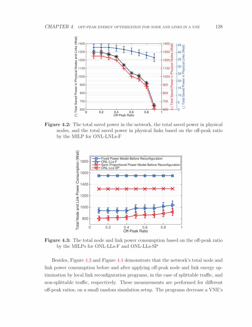
CHAPTER 4. OFF-PEAK ENERGY OPTIMIZATION FOR NODE AND LINKS IN A VNE 128
Off-Peak Ratio0 0.2 0.4 0.6 0.8 1
(*)
Tot
al S
aved
Pow
er in
Phy
sica
l Nod
es a
nd L
inks
(W
att)
600
700
800
900
1000
1100
1200
1300
1400
(.)
Tot
al S
aved
Pow
er in
Phy
sica
l Lin
ks (
Wat
t)
0
5
10
15
20
25
30
35
40
45
0 0.2 0.4 0.6 0.8 1
(+)
Tot
al S
aved
Pow
er in
Phy
sica
l Nod
es (
Wat
t)
600
700
800
900
1000
1100
1200
1300
1400
Figure 4.2: The total saved power in the network, the total saved power in physicalnodes, and the total saved power in physical links based on the off-peak ratioby the MILP for ONL-LNLs-F
Off-Peak Ratio0 0.2 0.4 0.6 0.8 1T
otal
Nod
e an
d Li
nk P
ower
Con
sum
ptio
n (W
att)
800
1000
1200
1400
1600
1800Fixed Power Model-Before ReconfigurationONL-LLs-FSemi Proportional Power Model-Before ReconfigurationONL-LLs-SP
Figure 4.3: The total node and link power consumption based on the off-peak ratioby the MILPs for ONL-LLs-F and ONL-LLs-SP
Besides, Figure 4.3 and Figure 4.4 demonstrate that the network’s total node and
link power consumption before and after applying off-peak node and link energy op-
timization by local link reconfiguration programs, in the case of splittable traffic, and
non-splittable traffic, respectively. These measurements are performed for different
off-peak ratios, on a small random simulation setup. The programs decrease a VNE’s

CHAPTER 4. OFF-PEAK ENERGY OPTIMIZATION FOR NODE AND LINKS IN A VNE 129
node and link energy consumption by reconfiguring only some of the virtual links.
The results prove that the formulated programs are able to save the power effectively,
for either splittable traffic or non-splittable traffic, based on both power models.
0 0.2 0.4 0.6 0.8 1
800
1000
1200
1400
1600
1800
Off−Peak Ratio
Tot
al N
ode
and
Link
Pow
er C
onsu
mpt
ion
(Wat
t)
Fixed Power Model−Before ReconfigurationONL−LLns−FSemi Proportional Power Model−Before ReconfigurationONL−LLns−SP
Figure 4.4: The total node and link power consumption based on the off-peak ratioby the BILPs for ONL-LLns-F and ONL-LLns-SP
The off-peak node and link energy optimization by local node and link reconfigura-
tion modifies the mapping for some of the both virtual nodes and links. Nonetheless,
the off-peak node and link energy optimization by local link reconfiguration adjusts
the mapping for only some of the virtual links. Hence, it is expected the formulated
programs for the first strategy save more energy than the defined programs for the
latter method. In this regard, we tested the formulated MILPs for ONL-LNLs-F
and ONL-LLs-F, on a small random simulation setup. Figure 4.5 illustrates that the
percentage of power the formulated MILPs for ONL-LNLs-F and ONL-LLs-F could
save on the range of off-peak ratio. The results confirm that the formulated MILP for
ONL-LNLs-F could save larger amounts of power in comparison to the defined MILP
for ONL-LLs-F. Although the local link reconfiguration strategy does not reconfigure
virtual nodes and therefore it saves smaller amounts of power in comparison to the
local node and link reconfiguration method, it causes fewer interruptions to the nor-
mal network operations. Note that, as Figure 4.5 reveals, the energy-saving ability of
ONL-LNLs-F is more sensitive to the off-peak ratio fluctuations in comparison to the

CHAPTER 4. OFF-PEAK ENERGY OPTIMIZATION FOR NODE AND LINKS IN A VNE 130
outcome of ONL-LLs-F. ONL-LNLs-F requires supporting both off-peak processing
and traffic demands, but since ONL-LLs-F does not modify virtual nodes mapping, it
only needs to handle the off-peak traffic demands. Therefore, the off-peak ratio vari-
ations have a greater impact on the energy-saving capability of ONL-LNLs-F rather
than ONL-LLs-F.
Off-Peak Ratio0 0.2 0.4 0.6 0.8 1T
otal
Sav
ed P
ower
in P
hysi
cal N
odes
and
Lin
ks (
%)
20
30
40
50
60
70
80
90ONL-LNLs-FONL-LLs-F
Figure 4.5: The total saved power in physical nodes and links based on the off-peakratio by the MILPs for ONL-LNLs-F and ONL-LLs-F
It is expected the programs save larger amounts of power when traffic is splittable,
because they are more flexible in terms of finding alternative paths. We checked this
issue on the formulated ILPs for off-peak node and link energy optimization by local
link reconfiguration. Figure 4.6 shows the percentage of power the formulated ILPs
for ONL-LLs-F and ONL-LLns-F could save in the defined range of off-peak ratio,
on a small random simulation setup. The results prove that the programs could save
more power when traffic is splittable in comparison to when traffic is non-splittable.
Note that ONL-LLs-F saves more power than ONL-LLns-F in the high off-peak ratios.
This is because, when off-peak ratio is low, it is easier for the programs to find the
alternative paths, and therefore ONL-LLs-F and ONL-LLns-F have almost the same
outcome. However, when off-peak ratio is high, it is more probable for the programs
to find the replaced paths by splitting high traffic loads into smaller loads.

CHAPTER 4. OFF-PEAK ENERGY OPTIMIZATION FOR NODE AND LINKS IN A VNE 131
Off-Peak Ratio0 0.2 0.4 0.6 0.8 1T
otal
Sav
ed P
ower
in P
hysi
cal N
odes
and
Lin
ks (
%)
28
30
32
34
36
38
40
42
44
46ONL-LLs-FONL-LLns-F
Figure 4.6: The total saved power in physical nodes and links based on the off-peakratio by the ILPs for ONL-LLs-F and ONL-LLns-F
Off-Peak Ratio0 0.2 0.4 0.6 0.8 1T
otsa
l Sav
ed P
ower
in P
hysi
cal N
odes
and
Lin
ks (
%)
24
26
28
30
32
34
36
38
40
42
44ONL-LLs-FONL-LLs-SP
Figure 4.7: The total saved power in physical nodes and links based on the off-peakratio by the MILPs for ONL-LLs-F and ONL-LLs-SP
Moreover, it is expected to save higher levels of power when Fixed power model is

CHAPTER 4. OFF-PEAK ENERGY OPTIMIZATION FOR NODE AND LINKS IN A VNE 132
applied, in comparison to when Semi-Proportional power model is employed, mainly
due to two reasons. First, a physical node or link, that is not fully utilized, consumes
a smaller amount of power when it is designed based on Semi-Proportional power
model, in comparison to when it is designed based on Fixed power model. Therefore,
by setting the same physical nodes and links into the sleep mode, the total amount of
saved power is smaller in the case of Semi-Proportional power model. Second, if the
energy-saving program sets a physical node into the sleep mode, then it re-allocates
its virtual nodes to other substrate nodes, and re-maps its respective virtual links to
alternative paths. In the case of Semi-Proportional power model, the re-allocated vir-
tual node and the rerouted traffic increase the power consumption over the alternative
physical nodes and links. However, in the case of Fixed power model, since the traffic
load does not affect a node or link’s power consumption, the reconfiguration does not
increase the power consumption over the alternative physical nodes and links. We
tested the formulated MILPs for ONL-LLs-F and ONL-LLs-SP on a small random
simulation setup in order to verify this expectation. The results in Figure 4.7 reveals
the percentage of saved power by MILPs for ONL-LLs-F and ONL-LLs-SP. Figure
4.7 confirms that the MILP for ONL-LLs-F could save larger amounts of power than
the MILP for ONL-LLs-SP.
Number of Virtual Networks0.5 1 1.5 2 2.5 3 3.5T
otsa
l Sav
ed P
ower
in P
hysi
cal N
odes
and
Lin
ks (
%)
20
25
30
35
40
45
50
55
60
65ONL-LLs-F
Figure 4.8: The total saved power in physical nodes and links based on the numberof involved virtual networks by the MILP for ONL-LLs-F

CHAPTER 4. OFF-PEAK ENERGY OPTIMIZATION FOR NODE AND LINKS IN A VNE 133
Furthermore, it is necessary to analyze the impact of different numbers of allo-
cated virtual networks over a substrate network, on the energy-saving ability of the
proposed solutions. In this regard, we measured the percentage of power the formu-
lated MILP for ONL-LLs-F could save on a small random simulation setup, when 1, 2
or 3 randomly generated virtual networks are allocated in the substrate network. The
off-peak ratio is assumed to be 0.5. The results are presented in Figure 4.8. Figure
4.8 reveals that increasing the number of allocated virtual networks in the substrate
network, decreases the total amount of power the program could save. Allocating a
new virtual network in a substrate network imposes several constraints to the pro-
grams, as new virtual nodes and links are mapped onto the physical nodes and links.
For instance, if a program wants to set a physical node into the sleep mode, then it
needs to re-allocate all the virtual nodes mapped onto the physical node, as well as
every virtual link passing the physical node. By allocating a new virtual network, the
program requires to find alternative physical nodes and paths for the newly mapped
virtual nodes and links. Therefore, the program is more limited, and its energy-saving
capability is degraded.
Number of Virtual Nodes per VN3.5 4 4.5 5 5.5 6 6.5T
otal
Sav
ed P
ower
in P
hysi
cal N
odes
and
Lin
ks (
%)
25
30
35
40
45
50
55ONL-LLs-F
Figure 4.9: The total saved power in physical nodes and links based on the numberof virtual nodes per VN by the MILP for ONL-LLs-F
It is also important to study the effect of different numbers of virtual nodes per

CHAPTER 4. OFF-PEAK ENERGY OPTIMIZATION FOR NODE AND LINKS IN A VNE 134
virtual network, on the energy-saving ability of the advised solutions. The number of
virtual nodes per VN expresses the size of virtual networks. Accordingly, we probed
the percentage of power saved by the formulated MILP for ONL-LLs-F on a small
random simulation setup, while the number of virtual nodes per VN varies between
4 and 6. The off-peak ratio is assumed to be 0.5. The results are displayed in Figure
4.9. Increasing the number of virtual nodes per VN, raises the number of allocated
virtual nodes in the physical nodes. Besides, adding virtual nodes in a virtual network
increases the number of virtual links in that virtual network. Consequently, incre-
menting the number of virtual nodes per VN imposes several new constraints to the
proposed energy-saving solutions, and makes them more limited in terms of setting
physical nodes and links into the sleep mode. Hence, as it is confirmed in Figure
4.9 for ONL-LLs-F, the program save smaller amounts of power when the number of
virtual nodes per VN is increased.
4.5.2 The Heuristic
On the other hand, it is essential to study the effectiveness of the proposed heuristic
algorithm for ONL-LLns-F. In this regard, first, we tested the heuristic algorithm on
a medium random simulation setup, and measured the network’s total node and link
power consumption before and after applying the heuristic algorithm, on the defined
range of off-peak ratio.
As discussed in Section 4.4, K affects the heuristic’s outcome. K is the number
of shortest paths the algorithm examines in order to find a single capable alternative
path for each re-mapped virtual link. The heuristic is simulated when K is 1, 2, 3, 4
or 5. The results are presented in Figure 4.10. The results confirm that the proposed
heuristic algorithm is able to reduce a VNE’s total node and link power consumption,
effectively. Besides, Figure 4.10 reveals that increasing the off-peak ratio decreases
the amount of power the heuristic could save. This is because increasing the off-peak
ratio raises the traffic load algorithm needs to re-allocate, and therefore the heuristic
is more limited in terms of finding alternative paths.
In addition, Figure 4.10 verifies increasing K raises the amount of power the
heuristic could save. If the heuristic needs to re-map a virtual link, then it finds K
shortest paths from the source node to the sink node of the virtual link in order to
provide a single qualified alternative path. However, the alternative path requires
satisfying some capacity constraints. In this regard, the shortest path (K = 1) might

CHAPTER 4. OFF-PEAK ENERGY OPTIMIZATION FOR NODE AND LINKS IN A VNE 135
not persuade the capacity constraints, but the second (K = 2) or third (K = 3)
shortest path may do. Consequently, the heuristic might save more power when K is
increased. Nevertheless, incrementing K increases the heuristic’s run time, because
it needs to find larger number of shortest paths. This is discussed theoretically in
Section 4.4. Besides, considering a specific off-peak ratio in Figure 4.10, the variations
in the saved amount of power by heuristic is decreasing when K is increasing. This
is because the number of available paths between two nodes in a substrate network
is limited, and by incrementing K the majority of possible paths are considered by
the heuristic, so it could not find new replaced paths. In consequence, a large enough
value of K, based on the substrate network size, makes it probable for the heuristic
to save the maximum amount of power in a VNE.
Off-Peak Ratio0 0.2 0.4 0.6 0.8 1T
otal
Nod
e an
d Li
nk P
ower
Con
sum
ptio
n (W
att)
3500
4000
4500
5000
5500
6000
Before ReconfigurationHeuristic (K=1)Heuristic (K=2)Heuristic (K=3)Heuristic (K=4)Heuristic (K=5)
Figure 4.10: The total node and link power consumption based on the off-peakratio before and after applying the heuristic with different values of K, forONL-LLns-F
It is vital to check the difference between the outcome of the formulated BILP for
ONL-LLns-F as the optimum result, and the proposed heuristic for the same problem.
This is tested on a small random simulation setup, and results are displayed in Figure
4.11. Figure 4.11 shows the percentage of power the BILP for ONL-LLns-F saves,
as well as the percentage of power the proposed heuristic for the same problem with
different values of K could save, on the defined range of off-peak ratio. Similar to

CHAPTER 4. OFF-PEAK ENERGY OPTIMIZATION FOR NODE AND LINKS IN A VNE 136
the results of previous simulation setup, increasing the off-peak ratio degrades the
ability of the BILP and the heuristic in terms of saving the power. Moreover, the
heuristic works closely to the optimum points set by the BILP, while the heuristic is
significantly faster than the BILP.
Off-Peak Ratio0 0.2 0.4 0.6 0.8 1T
otal
Sav
ed P
ower
in P
hysi
cal N
odes
and
Lin
ks (
%)
15
20
25
30
35
40
45
50
BILPHeuristic (k=1)Heuristic (k=2)Heuristic (k=3)Heuristic (k=4)
Figure 4.11: The total saved power in physical nodes and links based on the off-peakratio by the BILP and the heuristic with different values of K, for ONL-LLns-F
Additionally, we evaluated the impact of different numbers of mapped virtual
networks on a substrate network, on the heuristic’s outcome when K is 5 and the off-
peak ratio is 0.5. The number of allocated VNs is ranged from 1 to 3. The outcome
is presented for a medium random simulation setup in Figure 4.12. Similar to the
results shown in Figure 4.8, the results in Figure 4.12 confirms that increasing the
number of allocated virtual networks in the substrate network, limits the heuristic to
find replaced paths, and in consequence decreases the amount of power it could save.
The influence of different numbers of virtual node per virtual network, on the
heuristic’s outcome is also tested over a medium random simulation setup, and the
results are displayed in Figure 4.13. The off-peak ratio and K are assumed to be
0.5, and 5, respectively. Similar to the results displayed in Figure 4.9, the results in
Figure 4.13 verifies that incrementing the number of virtual nodes per mapped VN,
degrades the ability of the heuristic in terms finding alternative paths, and therefore
decreases the amount of power the heuristic could save.

CHAPTER 4. OFF-PEAK ENERGY OPTIMIZATION FOR NODE AND LINKS IN A VNE 137
Number of Virtual Networks0.5 1 1.5 2 2.5 3 3.5T
otal
Sav
ed P
ower
in P
hysi
cal N
odes
and
Lin
ks (
%)
15
20
25
30
35
40
45
50
55
60Heuristic (K=5)
Figure 4.12: The total saved power in physical nodes and links based on the numberof involved virtual networks by the heuristic with K = 5, for ONL-LLns-F
Number of Virtual Nodes per VN17 18 19 20 21 22 23T
otal
Sav
ed P
ower
in P
hysi
cal N
odes
and
Lin
ks (
%)
26
28
30
32
34
36
38
40
42Heuristic (K=5)
Figure 4.13: The total saved power in physical nodes and links based on the numberof virtual nodes per VN by the heuristic with K = 5 for ONL-LLns-F
Moreover, it is explained in Section 4.4 that the proposed heuristic, similar to the

CHAPTER 4. OFF-PEAK ENERGY OPTIMIZATION FOR NODE AND LINKS IN A VNE 138
formulated BILP for ONL-LLns-F, does not sleep the physical nodes with s2(vis) ≥
T , in order to decrease the traffic disruptions due to reconfiguration. Figure 4.14
studies the effect of changing s2 threshold on the capability of the heuristic when
K = 5, over a medium random simulation setup. The off-peak ratio is assumed as
0.5. Figure 4.14 shows that decreasing s2 threshold amount, decreases the amount
of power heuristic saves, because a smaller number of substrate nodes and links are
considered for power saving. Although decreasing s2 threshold decreases the amount
of power formulated solutions could save, it reduces the traffic interruptions to the
normal network operations, due to the reconfiguration.
T
0 0.2 0.4 0.6 0.8 1Tot
al S
aved
Pow
er in
Phy
sica
l Nod
es a
nd L
inks
(%
)
6
8
10
12
14
16
18
20
22
24
26
Heuristic (K=5)
Figure 4.14: The impact of different s2 thresholds on the total saved power inphysical nodes and links by the heuristic when K = 5 for ONL-LLns-F
It is expected this problem saves a larger amount of power in comparison to the
previously proposed solutions in Chapter 3. This is because the suggested methods
in Chapter 3 only concerns about a VNE’s link energy consumption, while physical
nodes consume more energy. We tested the proposed heuristic in this chapter and the
suggested heuristic in Chapter 3, on a medium simulation setup. The results in Figure
4.15 illustrate that the suggested heuristic in this chapter could save significantly
higher rates of the total power than the previously proposed heuristic.

CHAPTER 4. OFF-PEAK ENERGY OPTIMIZATION FOR NODE AND LINKS IN A VNE 139
Off-Peak Ratio0 0.2 0.4 0.6 0.8 1T
otal
Sav
ed P
ower
in P
hysi
cal N
odes
and
Lin
ks (
%)
0
5
10
15
20
25
30
35
40
45This HeuristicPrevious Heuristic
Figure 4.15: Comparison between the suggested heuristic in this chapter and pre-viously proposed heuristic in Chapter 3
Off-Peak Ratio0.1 0.2 0.3 0.4 0.5 0.6 0.7 0.8 0.9
Mea
n Li
nk U
tiliz
atio
n
0
0.2
0.4
0.6
0.8
1Peak TimeOff-Peak Time Before ReconfigurationOff-Peak Time after Reconfiguration
Figure 4.16: The mean link utilization based on the off-peak ratio over differentconfigurations
Besides, rerouting the traffic to the other substrate paths causes changes to the
links’ utilization. The heuristic algorithm re-maps the off-peak traffic onto the other
paths in order to save energy. Accordingly, it is needed to make sure the increased
utilization is controlled and does not cause congestion. The link utilization for three
different configurations is measured on a medium random simulation setup, and the

CHAPTER 4. OFF-PEAK ENERGY OPTIMIZATION FOR NODE AND LINKS IN A VNE 140
average results are shown in Figure 4.16. The first configuration is for the peak
time when the allocated bandwidth is able to handle “Worst-Case” scenarios. The
second configuration is for the off-peak period while no energy-saving algorithm is
implemented. Over this period the links are less utilized while the same bandwidth
capacity is allocated and consume the same power as the peak time. After applying
our suggested heuristic when K = 5 and the off-peak ratio is 0.5, the average link
utilization is increased, but it is still less than the maximum utilization. Note that
the link utilization shown in Figure 4.16 is the mean of the maximum points of all
the test scenarios.
Number of Virtual Nodes per VN5 6 7 8 9 10
Run
Tim
e (S
ec)
0
500
1000
1500
2000
2500
3000
3500
4000
HeuristicBILP
6 8 100
0.1
0.2
0.3
Figure 4.17: Required run time based on the different number of virtual nodes perVN, for the BILP and the heuristic with K = 5, for ONL-LLns-F
The formulated BILP for ONL-LLns-F is NP-hard, while the complexity of the
proposed heuristic algorithm for the same problem is O(K|Vs||Φ||Emv |(|Vs|2log|Vs| +
|Es|2|Φ||Emv |+ |Vs||Es||Φ||Em
v |)). So, it is expected the proposed heuristic needs less
run time in comparison to the formulated binary integer linear program for the same
problem. We verified run time for the BILP and the heuristic on a single random
scenario. This scenario includes a random substrate topology with 15 physical nodes,
while 2 random virtual networks are mapped onto the substrate network, and the
off-peak ratio is assumed to be 0.5. We probed the required run time for the BILP
and the heuristic with K = 5, while the number of virtual nodes per virtual network

CHAPTER 4. OFF-PEAK ENERGY OPTIMIZATION FOR NODE AND LINKS IN A VNE 141
is changing from 5 to 10. The number of virtual nodes per VN expresses the size of
virtual networks. As the results in Figure 4.17 show, the heuristic needs considerably
lower run time in comparison to the BILP. Besides, Figure 4.17 confirms that enlarging
the size of mapped virtual networks, increases the required run time for both the
heuristic and the BILP. Note that the number of nodes per virtual network affects
the number of virtual links per virtual network, and this impacts the time complexity
of the heuristic. However, since the BILP is NP-hard, its required run time changes
almost exponentially by changing the number of virtual nodes per VN.
The simulation results prove the suggested energy-saving solutions are able to
reduce a VNE’s node and link energy consumption, during the off-peak period, ef-
fectively. Besides, the proposed heuristic is a simple and fast algorithm that works
closely to the optimum points.
Note that every simulation setup is quite large to cover a substantial number
of random topologies in order to verify the effectiveness of the proposed solutions.
Besides, the calculated confidence intervals confirm that the results are precise enough
to reveal the significances of the different energy-saving methods.
4.6 Summary
In this chapter, we have formulated multiple novel ILPs that optimize the node and
link energy consumption in a VNE during the off-peak period, by reconfiguring the
mapping for some of the mapped virtual nodes and links. They are developed accord-
ing to two power models, and considering the impact of traffic splittability. Because
the formulated ILPs are NP-hard, we also suggested a novel energy-saving heuristic
algorithm. The defined ILPs and the heuristic are tested over randomly generated
VNEs. Simulation results show that the proposed solutions are noticeably effective
and the heuristic works closely to the optimum points.

Chapter 5
GreenMap: Green Mapping of
Heterogeneous MapReduce-based Virtual
Networks onto a Data Center Network
and Controlling Incast Queueing Delay
5.1 Introduction
The cloud computing is becoming widespread, and the energy consumption of the
physical infrastructure that provides resources for a cloud is growing [93]. Accordingly,
the energy management is a key challenge for data centers to reduce all their energy-
related costs [94].
MapReduce [95] is a cloud computing approach that parallelizes a computation
across a large-scale cluster of servers. We target MapReduce, because it is widely
deployed in many data centers like Google [96], Yahoo!, Amazon, and Facebook [97].
More than ten thousands distinct MapReduce programs, with the average of one
hundred thousand MapReuce jobs per day, have been executed at Google [96]. In
this framework, users specify the computation tasks by generating map and reduce
functions. Nodes that perform a mapping job are called mappers. Mappers process
input data and generate intermediate key and value pairs. The generated key and
value pairs are shuffled through shuffler nodes to the other nodes that perform a
reducing job, called reducers. Reducers aggregate the received intermediate key and
value pairs from different mappers and compute the computational results for an
application.
VNs together with VMs underpin Virtualized Data Centers (VDCs). A VDC
142

CHAPTER 5. GREENMAP 143
in the virtual layer consists of virtual networks in which VMs are connected with
virtual links by virtual switches/routers. In the substrate layer, it consists of a data
center network in which physical servers are connected with physical links by physical
switches/routers. A VDC embedding process maps requested virtual nodes and links
onto physical nodes and paths of a data center network, respectively. Note that a
VDC embedding process is a type of discussed VNE embedding processes, in which
the substrate network is a data center network.
Traditional data centers are moving toward virtualized data centers in order to
address their limitations regarding the network performance, security, and manage-
ability [16]. Accordingly, in this chapter, we consider MapReduce-based virtual net-
works in VDCs. Each virtual network is heterogeneous, where a virtual node might
be a mapper, a reducer, or a shuffler in a MapReduce framework. The data center
network is also heterogeneous, with a multi-level topology such as a tree or a fat-tree.
A substrate node could be a server, or a switch/router. In this case, a VDC embed-
ding process requires to split computation-based virtual nodes (mappers/reducers)
and embed them onto multiple physical servers, in order to parallelize the compu-
tation tasks. Nevertheless, all the existing embedding methods for virtual networks,
e.g. [16, 29, 32, 38, 60, 62, 64, 69, 98, 99] assume that a virtual node could be mapped
only onto a single substrate node. Moreover, none of them provides a tool that could
handle the heterogeneity of MapReduce-based VNs and the data center network.
Therefore, they are not able to map the heterogeneous MapReduce-based VNs onto
the heterogeneous data center network.
Incast traffic pattern in a data center network firstly introduced in [100]. In a
MapReduce framework, multiple mappers may simultaneously send intermediate key
and value pairs to a single reducer. Therefore, the bottleneck physical link over the
physical path to the reducer will likely be congested. In non-virtualized data centers,
the incast congestion normally happens in the bottleneck physical link that connects
a shallow-buffered Top-of-Rack (ToR) switch to an end-server that hosts a reducer
[101–105]. The converged traffic flows deplete either the switch’s memory or the
maximum allowed for that interface, resulting in packet loss [102]. The incast traffic
also may cause a long queuing delay called incast queueing delay [102]. MapReduce
requirements for low latency are directly related to the quality of the result returned
and thus the revenue. Consequently, it is vital for the providers to control the incast
delay.

CHAPTER 5. GREENMAP 144
The incast problem in VDCs is different from the incast problem in non-virtualized
(traditional) data centers. During a VDC embedding process, a specific amount of
bandwidth capacity is allocated to each virtual link in substrate paths. The traffic
flows in the allocated paths are limited to their assigned bandwidth capacity. Hence,
the incast problem might happen over the bottleneck allocated paths to virtual links.
In this case, the incast traffic may face the incast queuing delay in multiple physical
links over the bottleneck allocated path, leading to a longer incast queuing delay in
the virtual link. This problem is significantly different from the scenario when incast
happens only in a single bottleneck physical link, which connects a ToR switch to an
end-server, in the case of non-virtualized data centers. To the best of our knowledge
this problem is not introduced in any existing research studies.
The existing research studies on the incast problem, for non-virtualized networks,
are focused on creating new traffic control mechanisms, and updating Transmission
Control Protocol (TCP). They either tried to decrease the packet loss by increasing
the memory of shallow-buffered switches [102,106,107], or increase the recovery speed
of TCP by decreasing the value of Retransmission Timeout (RTO) [104, 106, 108].
Nonetheless, the existing solutions for the incast problem are not efficient, and traffic
control algorithms alone are difficult to mitigate the incast congestion [105]. Besides,
they do not provide a solution for the incast problem in VDCs.
In this chapter, we propose GreenMap, an energy-efficient embedding method for
MapReduce-based virtual networks that also controls the incast queuing delay. We
formulate a Mixed Integer Disciplined Convex Program (MIDCP) for this problem.
Since the formulated MIDCP is NP-hard, it is not scalable to large network sizes.
Therefore, we also propose a novel and scalable heuristic for GreenMap. Both of
the MIDCP and the heuristic map heterogeneous MapReduce-based VNs onto the
heterogeneous data center network. They minimize a VDC’s total consumed energy
by physical servers, physical switches/routers, and physical links. They also control
the incast queuing delay.
In this regard, we may split computation-based virtual nodes and map them onto
multiple server substrate nodes. Accordingly, we address the emerged challenge of
splitting and mapping adjacent virtual links of splitted and mapped virtual nodes.
We might also collocate multiple splitted computation-based virtual nodes of a VN
in a single server substrate node. The shuffler virtual nodes are assumed to be in the
core/aggregation level in a data center network with a multi-level topology. Besides,

CHAPTER 5. GREENMAP 145
shuffler virtual nodes do not perform large computation tasks, and therefore there
is no need of parallel computations in this case. Thus, we do not split a shuffler
virtual node. A shuffler virtual node is mapped only onto a single switch/router
substrate node. But, we may collocate multiple shuffler virtual nodes of a VN in a
single switch/router substrate node. Note that the substrate path that connects an
allocated computation-based virtual node in a server substrate node to an allocated
shuffler virtual node in a switch/router substrate node, or vice versa, may traverse
through multiple relay switches/routers.
Our method also controls the introduced incast queueing delay in any adjacent
virtual link of a mapped reducer virtual node. This is achieved by calculating the
average end-to-end queueing delay for the incast traffic pattern during the virtual
link mapping process. The incast queueing delay in an adjacent virtual link of an
embedded reducer virtual node is related to the mentioned challenge of virtual link
mapping. We demonstrate how controlling the incast queueing delay impacts the
embedding process, the level of energy-saving, and the network’s admittance ratio.
We evaluated both the MIDCP and the heuristic for GreenMap over randomly
generated VDC scenarios. Simulation results prove the MIDCP and the heuristic save
larger amounts of energy in the data center network than an existing energy-efficient
embedding method for VNs that do not allow virtual node splitting. Besides, the
simulations confirm that the incast queueing delay is controlled, and illustrate the
influence of controlling the incast queueing delay on the energy-saving rates and the
network’s admittance ratio. It is also demonstrated that the heuristic could achieve
closely to the optimum points set by the MIDCP.
In this regard, our contributions in this chapter are:
• The problem is formulated as an MIDCP.
• A novel and scalable heuristic is also proposed for the problem that can achieve
closely to the optimum points.
• Different from [16,29,32,38,60,62,64,69,98,99], our approach makes it probable
to split and map computation-based virtual nodes onto the data center network.
Accordingly, it enables the providers to embed computation-based VNs onto a
data center network.
• Different from [16, 29, 32, 38, 60, 62, 64, 69, 98, 99], our solution handles the het-
erogeneity of MapReduce-based VNs and the data center network.

CHAPTER 5. GREENMAP 146
• For the first time, we introduce a new incast problem for virtualized data centers.
• We demonstrate a novel approach that controls the introduced incast queueing
delay.
• We tackle the incast problem during the provisioning process. So, it prevents
the incast problem from happening at the first point. This is a considerably
more efficient approach than the existing solutions for the incast in [102,104,106,
106–108] that attempt to recover the connection after that the incast happens.
• We examine both the MIDCP and the heuristic through extensive simulations,
and check impacts of different factors.
• We demonstrate how controlling the incast queueing delay may affect the
energy-saving level and the network’s admittance ratio.
• To the best of our knowledge, this is the first study on the energy-efficient
embedding of MapReduce-based virtual networks onto a data center network.
The rest of this chapter is organized as follows: We define our network model in
Section 5.2, and study related power models in Section 5.3. The MIDCP and the
heuristic for GreenMap are formulated in Section 5.4, and Section 5.5, respectively.
The performance of the solutions is evaluated in Section 5.6. This chapter concludes
in Section 5.7.
5.2 The Network Model
We consider a heterogeneous data center network with a multi-level topology, such
as a tree or a fat-tree, as the substrate network. It is modeled as a directed graph
Gs = (Vs, Es). The directed graph provides a higher level of flexibility in regard
to routing traffic flows. Vs and Es denote the set of substrate nodes and substrate
links, respectively. The ith substrate node vis could be a server, or a switch/router.
The ith substrate node, which is a server, is represented by vis. Cc(vis) is the Central
Processing Unit (CPU) capacity of vis. Vs denotes the set of server substrate nodes.
Moreover, the ith substrate node, which is a switch/router, is represented by vis.
Cb(vis) is the switching capacity of vis. Vs denotes the set of switch/router substrate
nodes. Therefore, Vs = {Vs ∪ Vs}.

CHAPTER 5. GREENMAP 147
A substrate link li,js in the data center network connects the ith substrate node to
the jth substrate node. Cb(li,js ) is the bandwidth capacity of li,js .
Figure 5.1: Example: A MapReduce-based VN’s topology
The nth virtual network is modeled as a directed graph Gn = (Vn, En), where Vn
and En denote the set of virtual nodes and virtual links in the nth VN, respectively.
Φ is the set of all of the VNs, and Ln = |En|. Figure 5.1 shows an example of a
MapReduce-based VN’s topology. In this framework, the kth virtual node vkn in the
nth VN could be a mapper, a reducer, or a shuffler. The kth virtual node in the nth
VN, which is a mapper, is represented by vkn. Cc(vkn) is the requested CPU capacity
for vkn. VN customers may specify the minimum Cmc (vkn) and the maximum Cm
c (vkn)
amount of required CPU capacity per allocated physical machine for vkn. We assume
that a mapper virtual node vkn generates traffic that follows Poisson process with the
mean rate of λ(vkn). Considering Vn as the set of mapper virtual nodes in the nth
VN, λMn is equal to
∑k∈Vn
λ(vkn). Besides, the kth virtual node in the nth VN, which
is a reducer, is represented by vkn. Cc(vkn) is the demanded CPU capacity for vkn. VN
customers also may specify the minimum Cmc (vkn) and the maximum Cm
c (vkn) amount
of required CPU capacity per allocated physical machine for vkn. Vn denotes the set
of reducer virtual nodes in the nth VN. Furthermore, the kth virtual node in the nth
VN, which is a shuffler, is represented by vkn. We assume that a shuffler virtual node
vkn only has the switching capacity demand Cb(vkn), that is equal to the summation of
its adjacent virtual links’ bandwidth demands. Vn denotes the set of shuffler virtual

CHAPTER 5. GREENMAP 148
nodes in the nth VN. Therefore, Vn = {Vn ∪ Vn ∪ Vn}.The set of virtual links are presented as a set of ordered virtual node pairs
lam,bm
n ,m = 1, 2, . . . , Ln. am and bm are the source and the sink virtual nodes of
the mth virtual link in the corresponding VN, respectively. Cb(lam,bm
n ) is the band-
width demand of lam,bm
n . We presume computation-based virtual nodes are connected
through shuffler virtual nodes in a virtual network topology. In other words, there is
no pair of computation-based virtual nodes that are connected directly to each other
in a VN topology. This is the real case in a MapReduce framework.
5.3 Power Models
Considering the heterogeneous data center network as the substrate network, we
have three major power consumers, physical servers, physical switches/routers, and
physical links. In this chapter, we intend to minimize the total consumed energy by
them in a VDC. We study a power model for each of these substrate elements.
Equation 5.1 defines the actual power consumption p(vis) for a server substrate
node vis [58]. α(vis) denotes the status of vis. It is 1, if v
is is active. Otherwise, it is 0.
pb(vis) is the base power consumption of vis required to keep it active. pm(vis) is the
maximum power consumption of vis. The total allocated processing capacity φ(vis) to
computation-based virtual nodes in vis changes its actual power consumption between
pb(vis) and pm(vis), linearly. pb(vis) and pm(vis) could be found through calibration
experiments, e.g. in [59].
p(vis) = α(vis)pb(vis) +
φ(vis)
Cc(vis)
(pm(vis)− pb(vis)
)(5.1)
Equation 5.2 defines the actual power consumption p(vis) for a switch/router sub-
strate node vis [56]. α(vis) shows the status of vis. pb(vis) and pm(vis) are the base
and the maximum power consumption of vis, respectively. The total traffic load r(vis)
in vis changes its actual power consumption between its base and maximum power
consumption, linearly.
p(vis) = α(vis)pb(vis) +
r(vis)
Cb(vis)
(pm(vis)− pb(vis)
)(5.2)
According to [56], pb(vis) is 0.85Cb(vis)
23 , and pm(vis) is Cb(v
is)
23 . Consequently,

CHAPTER 5. GREENMAP 149
Equation 5.2 is rewritten in Equation 5.3.
p(vis) = 0.85α(vis)Cb(vis)
23 +
0.15r(vis)
Cb(vis)13
(5.3)
Similarly, Equation 5.4 defines the actual power consumption p(li,js ) of a substrate
link li,js [56]. pb(li,js ) and pm(li,js ) are the base and the maximum power consumption of
li,js , respectively. The total allocated traffic capacity r(li,js ) to virtual links in li,js varies
its actual power consumption, linearly. Note that pb(li,js ) and pm(li,js ) are normally
defined for different ranges of link bandwidth capacity, based on the link’s length and
the type of the cable. Some numerical amounts for them are given in [56].
p(li,js ) = α(li,js )pb(li,js ) +r(li,js )
Cb(li,js )
(pm(li,js )− pb(li,js )
)(5.4)
According to the above defined power models, the most effective way of saving
energy in any of the mentioned substrate elements is shutting down the device. Note
that the same amount of processing/traffic demand might cause different amounts
of power consumption in distinct substrate elements, based on the element’s pro-
cessing/bandwidth capacity, its base power consumption, and its maximum power
consumption.
5.4 The Mixed Integer Disciplined Convex Pro-
gram
In this problem, the processing/bandwidth capacity of every substrate node, and the
bandwidth capacity of every substrate link are given. Besides, each VN’s topology, the
processing/bandwidth demand of every virtual node and their minimum/maximum
processing demands per physical server, the bandwidth demand of every virtual link,
and λ(vkn) of each mapper virtual node are known. We need to find a mapping for
every VN such that the data center network’s total energy consumption by physical
servers, physical switches/routers, and physical links, is minimized. We also require
to control the incast queuing delay according to the given D, which is the maximum
tolerable queuing delay in a virtual link.

CHAPTER 5. GREENMAP 150
As it is discussed, we may split the computation-based virtual nodes and em-
bed them onto multiple physical servers. But, we map a shuffler virtual node
onto a single physical switch/router. We also may collocate virtual nodes (map-
pers/reducers/shufflers) of a VN in a single relevant substrate node. A new challenge
will emerge in this model. The issue is what is the bandwidth capacity that needs to
be allocated to an adjacent virtual link of a splitted and mapped computation-based
virtual node. Likely, a splitted computation-based virtual node processes propor-
tional traffic to its assigned processing capacity. Therefore, the amount of bandwidth
we allocate to an adjacent virtual link of a splitted and mapped computation-based
virtual node is proportional to its assigned processing capacity. Thus, in this model,
more likely the introduced incast problem may arise in an adjacent virtual link of a
splitted reducer virtual node. Note that in order to avoid out of order packet delivery,
we do not split generated traffic of an allocated virtual node.
In order to control the introduced incast queueing delay, it is required to find the
end-to-end queuing delay for the incast traffic pattern in the substrate path allocated
to every virtual link terminates at a splitted and mapped reducer virtual node. In the
incast traffic pattern, λMn is the mean traffic rate in the substrate path. The majority
of today’s switches/routers are internally non-blocking (i.e. the internal switch fabric
speed is considerably faster than each output port). Therefore, traffic can only be
blocked by limited bandwidths of output ports which are defined earlier by the link
bandwidth capacity. We model the queue of an allocated bandwidth capacity to a
virtual link in a substrate link by M/M/1 queue. According to Jackson Networks
theorem and because we do not split generated traffic of an allocated virtual node,
the end-to-end incast queuing delay in the substrate path could be calculated by
knowing the amount of allocated traffic capacity to the virtual link in each physical
link over the substrate path, and λMn . Since the amount of bandwidth we allocate
to the virtual links are proportional to the assigned capacity of its end virtual nodes,
the way we split reducer virtual nodes directly impacts the incast queueing delay.
Besides, the substrate node which we map the splitted reducer virtual node onto, and
accordingly the allocated substrate path to each of the adjacent virtual links, also may
influence the incast queuing delay. Clearly, this limits the level of freedom regarding
the energy-efficient embedding of the VNs, and may affect the energy-saving rate and
the network’s admittance ratio.
Considering the discussed definitions, we formulate the following MIDCP as a

CHAPTER 5. GREENMAP 151
solution for GreenMap:
Optimization Variables:
• φ(vkn, vis) is a real variable. It represents a fraction of processing/switching
demand of a virtual node vkn, that is allocated in a substrate node vis. vkn could
be vkn, vkn, or v
kn. v
is could be vis or v
is.
• α(vis), α(vis), and α(li,js ) are binary variables. They denote the status of re-
spective substrate node/link. The variable is 1 in the case the device is active.
Otherwise, it is 0.
• α(vkn, vis), α(v
kn, v
is), α(v
kn, v
is) are binary variables denote whether a virtual node
is allocated in a substrate node (the variable is 1), or not (the variable is 0).
• α(lx,yn (m)) is a binary variable. It is 1, if the whole or a fraction of vam
n ’s
processing/switching demand is allocated in vxs , and the whole or a fraction of
vbm
n ’s processing/switching demand is allocated in vys . Otherwise, it is 0. lx,yn (m)
is a sub virtual link of lam,bm
n that connects the allocated source virtual node in
vxs to the allocated sink virtual node in vys .
• zi,j(lx,yn (m)) is a binary variable. It is 1 if the allocated substrate path for lx,yn (m)
passes through li,js . Otherwise, it is 0.
• dx,yn (m) is a real variable. It is a fraction of Cb(lam,bm
n ) that needs to be allocated
to lx,yn (m).
• di,j(lx,yn (m)) is a real variable. It shows the amount of allocated traffic capacity
to lx,yn (m) in li,js .
Objective Function: Our objective is minimizing the total consumed energy by phys-
ical servers, physical switches/routers, and physical links, in a VDC. Equation 5.5
maintains this objective.
Minimize{∑
i∈Vs
α(vis)pb(vis) +
φ(vis)
Cc(vis)
(pm(vis)− pb(vis)
)+∑i∈Vs
0.85α(vis)Cb(vis)
23 +
0.15r(vis)
Cb(vis)13
+∑
(i,j)∈Es
α(li,js )pb(li,js ) +r(li,js )
Cb(li,js )
(pm(li,js )− pb(li,js )
)}(5.5)

CHAPTER 5. GREENMAP 152
Constraints: Every virtual node must be mapped onto one or multiple substrate
nodes. This is ensured by the first constraint in Equation 5.6. Note that this con-
straint allows collocation of multiple virtual nodes of a VN onto a single substrate
node. The constraint in Equation 5.7 prevents a computation-based virtual node
from being mapped onto a switch/router substrate node. Besides, the constraint in
Equation 5.8 forbids a shuffler virtual node to be mapped onto a server substrate
node. ∑i∈Vs
φ(vkn, vis) = 1 , ∀n ∈ {n|Gn ∈ Φ}, ∀k ∈ Vn (5.6)
∑n∈{n|Gn∈Φ}
(∑k∈Vn
φ(vkn, vis) +
∑k∈Vn
φ(vkn, vis))= 0, ∀i ∈ Vs (5.7)
∑n∈{n|Gn∈Φ}
∑k∈Vn
φ(vkn, vis) = 0 , ∀i ∈ Vs (5.8)
The allocated processing capacity to a computation-based virtual node in a server
substrate node must be equal or greater than the requested minimum CPU capac-
ity per physical machine for the virtual node, and equal or less than the requested
maximum CPU capacity per physical machine for the virtual node. This is confirmed
in the constraint in Equation 5.9 for mapper virtual nodes, and in the constraint in
Equation 5.10 for reducer virtual nodes. Note that the given ratio must be feasible.
For example, Cmc (vkn)
Cc(vkn)can not be greater than 0.5.
Cmc (vkn)
Cc(vkn)α(vkn, v
is) ≤ φ(vkn, v
is) ≤
Cmc (vkn)
Cc(vkn)α(vkn, v
is) ,
∀i ∈ Vs, ∀n ∈ {n|Gn ∈ Φ}, ∀k ∈ Vn (5.9)
Cmc (vkn)
Cc(vkn)α(vkn, v
is) ≤ φ(vkn, v
is) ≤
Cmc (vkn)
Cc(vkn)α(vkn, v
is) ,
∀i ∈ Vs, ∀n ∈ {n|Gn ∈ Φ}, ∀k ∈ Vn (5.10)
The constraint in Equation 5.11 restricts the program to map a shuffler virtual node
only onto one switch/router substrate node.
φ(vkn, vis) = α(vkn, v
is), ∀i ∈ Vs, ∀n ∈ {n|Gn ∈ Φ}, ∀k ∈ Vn (5.11)

CHAPTER 5. GREENMAP 153
Besides, the total allocated processing capacity to computation-based virtual nodes in
a server substrate node must be equal or less than the substrate node’s CPU capacity,
as shown in the constraint in Equation 5.12. The total allocated switching capacity
to shuffler virtual nodes in a switch/router substrate node also must be equal or
less than the substrate node’s switching capacity, as indicated in the constraint in
Equation 5.13.
∑n∈{n|Gn∈Φ}
(∑k∈Vn
φ(vkn, vis)Cc(v
kn)+
∑k∈Vn
φ(vkn, vis)Cc(v
kn))≤ Cc(v
is) , ∀i ∈ Vs (5.12)
∑n∈{n|Gn∈Φ}
∑k∈Vn
φ(vkn, vis)Cb(v
kn) ≤ Cb(v
is) , ∀i ∈ Vs (5.13)
In the next step, the program needs to map the adjacent virtual links of the allocated
virtual nodes. We discussed that computation-based virtual nodes are connected
through shuffler virtual nodes in a VN topology. So, we have two types of virtual
links in a VN. First, a virtual link that connects a computation-based virtual node to a
shuffler virtual node, or vice versa. Second, a virtual link that connects a shuffler vir-
tual node to another shuffler virtual node. Therefore, φ(vam
n , vxs )φ(vbm
n , vys )Cb(lam,bm
n )
is the fraction of Cb(lam,bm
n ) that needs to be allocated to lx,yn (m). This amount is
proportional to the assigned processing/switching capacity to the mapped source and
sink virtual nodes of the virtual link lam,bm
n . Accordingly, the linear constraints in
Equation 5.14 force dx,yn (m) to take the value of φ(vam
n , vxs )φ(vbm
n , vys ).
dx,yn (m) ≤ φ(vam
n , vxs ) ,
dx,yn (m) ≤ φ(vbm
n , vys ) ,
dx,yn (m) ≥ φ(vam
n , vxs ) + φ(vbmn , vys )− 1 ,
dx,yn (m) ≥ 0 ,
∀x ∈ Vs, ∀y ∈ Vs, ∀n ∈ {n|Gn ∈ Φ},m = 1, . . . , Ln (5.14)
B1, B2, B3, and B4 are large integer numbers. They must be large enough to be greater
than the largest amount of the left-hand side of their respective inequality. If there is
a non-zero bandwidth demand for lx,yn (m), then the first constraint in Equation 5.15
forces α(lx,yn (m)) to be 1. Then, the second constraint in Equation 5.15 needs to route
a single unit of data from the xth substrate node to the yth substrate node. Because

CHAPTER 5. GREENMAP 154
the variable zi,j(lx,yn (m)) is binary, the unit of data could not be splitted. Besides,
the third constraint in Equation 5.15 limits the program routing, so the maximum
number of incoming and outgoing flows for a sub virtual link, in any substrate node,
is two. This maintains a single loopless path. The driven route will be used as the
substrate path for lx,yn (m). Note that if α(lx,yn (m)) = 0, then no substrate path is
allocated to lx,yn (m).
dx,yn (m)Cb(lam,bm
n ) ≤ B1α(lx,yn (m)) ,
∑{j|(i,j)∈Es}
zi,j(lx,yn (m))−∑
{j|(j,i)∈Es}zj,i(lx,yn (m)) =
⎧⎪⎪⎪⎪⎨⎪⎪⎪⎪⎩
α(lx,yn (m)) if i = x
−α(lx,yn (m)) if i = y
0 otherwise
,
∑{j|(i,j)∈Es}
zi,j(lx,yn (m)) +∑
{j|(j,i)∈Es}zj,i(lx,yn (m)) ≤ 2,
∀i ∈ Vs, ∀x ∈ Vs, ∀y ∈ Vs, ∀n ∈ {n|Gn ∈ Φ},m = 1, . . . , Ln (5.15)
Furthermore, the total allocated traffic capacity r(li,js ) in a substrate link li,js must
be less than its physical bandwidth capacity Cb(li,js ), as expressed in the con-
straint in Equation 5.16. r(li,js ) is the summation of every allocated traffic ca-
pacity di,j(lx,yn (m)) to a sub virtual link lx,yn (m) in li,js . di,j(lx,yn (m)) is equal to
zi,j(lx,yn (m))dx,yn (m)Cb(lam,bm
n ). If the allocated substrate path to lx,yn (m) passes
through li,js , then zi,j(lx,yn (m)) is 1, and therefore di,j(lx,yn (m)) is dx,yn (m)Cb(lam,bm
n ).
Otherwise, di,j(lx,yn (m)) is 0. The linear constraints in Equation 5.17 force di,j(lx,yn (m))
to take the value of zi,j(lx,yn (m))dx,yn (m)Cb(lam,bm
n ). Note that M is the largest virtual
link bandwidth demand in Φ.
r(li,js ) ≤ Cb(li,js ) , ∀(i, j) ∈ Es, where:
r(li,js ) =∑x∈Vs
∑y∈Vs
∑n∈{n|Gn∈Φ}
Ln∑m=1
di,j(lx,yn (m)) (5.16)
di,j(lx,yn (m)) ≤ Mzi,j(lx,yn (m)) ,

CHAPTER 5. GREENMAP 155
di,j(lx,yn (m)) ≤ dx,yn (m)Cb(lam,bm
n ) ,
di,j(lx,yn (m)) ≥ dx,yn (m)Cb(lam,bm
n )−M(1− zi,j(lx,yn (m))) ,
di,j(lx,yn (m)) ≥ 0 ,
∀(i, j) ∈ Es, ∀x ∈ Vs, ∀y ∈ Vs, ∀n ∈ {n|Gn ∈ Φ} ,m = 1, . . . , Ln (5.17)
Moreover, the total incoming and outgoing traffic of a switch/router substrate node
must be less than its switching capacity. This is confirmed in the constraint in
Equation 5.18.
r(vis) ≤ Cb(vis) , ∀i ∈ Vs , where:
r(vis) =∑
(i,j)∈Es
r(li,js ) +∑
(j,i)∈Es
r(lj,is ) (5.18)
Considering M/M/1 queue and Jackson Networks theorem, and because we do not
split generated traffic by an allocated virtual node, the average end-to-end incast
queuing delay of a sub virtual link lx,yn (m) could be calculated by the sum of1
μ(lx,yn (m))−λMn
for every substrate link li,js that a traffic capacity is allocated to lx,yn (m)
in it (zi,j(lx,yn (m)) = 1). The mean service rate μ(lx,yn (m)) for lx,yn (m) is equal to
dx,yn (m)Cb(lam,bm
n ).
Considering the continuous function f(g, h) = g2
h, h > 0, the hessian matrix H
of f is shown in Equation 5.19. Eigenvalues of H are 0 and 2g2+2h2
h3 . Because all
eigenvalues of H are non-negative, H is positive semi-definite. Therefore, f is jointly
convex on both g and h.
H =
⎡⎢⎣ 2
h−2gh2
−2gh2
2g2
h3
⎤⎥⎦ (5.19)
Thus, the left-hand side of the first inequality constraint in Equation 5.20 calculates
the end-to-end incast queueing delay in the allocated substrate path to a sub virtual
link that connects a mapped shuffler virtual node to a mapped and splitted reducer
virtual node. Note that if no traffic capacity is allocated to a sub virtual link lx,yn (m)
in a substrate link li,js , then zi,j(lx,yn (m)) is 0, and therefore the delay is 0. 2(1 −α(lx,yn (m))) is added to ensure the denominator is never 0. According to the first
constraint in Equation 5.15, if dx,yn (m) is greater than 0, then α(lx,yn (m)) is 1, and
therefore the denominator is dx,yn (m)Cb(lam,bm
n )−λMn . Otherwise, if dx,yn (m) is 0, then

CHAPTER 5. GREENMAP 156
zi,j(lx,yn (m)) of any substrate link is 0, and the denominator is λMn .
Hence, the first inequality constraint in Equation 5.20 is a mixed integer disciplined
convex constraint [109], which verifies the incast queueing delay in the allocated
substrate path to every virtual link that terminates at a mapped reducer virtual
node, is less than D. Besides, the second constraint in Equation 5.20 confirms that
every queue in the network is stable.
∑(i,j)∈Es
zi,j(lx,yn (m))2
dx,yn (m)Cb(lam,bmn )− λM
n + 2 (1− α(lx,yn (m)))λMn
≤ D,
dx,yn (m)Cb(lam,bm
n ) > α(lx,yn (m))λMn ,
∀n ∈ {n|Gn ∈ Φ},m ∈ {m|m = 1, . . . , Ln; bm ∈ Vn}, ∀x ∈ Vs , ∀y ∈ Vs (5.20)
The constraints in Equation 5.21 check the respective device’s status.
φ(vis) ≤ B2α(vis) , ∀i ∈ Vs , where:
φ(vis) =∑n∈Gn
(∑k∈Vn
φ(vkn, vis)Cc(v
kn) +
∑k∈Vn
φ(vkn, vis)Cc(v
kn));
r(vis) ≤ B3α(vis) , ∀i ∈ Vs;
r(li,js ) ≤ B4α(li,js ) , ∀(i, j) ∈ Es (5.21)
Besides, the variables must hold the following bounds:
0 ≤ φ(vkn, vis) ≤ 1, ∀i ∈ Vs, ∀n ∈ {n|Gn ∈ Φ}, ∀k ∈ Vn
α(vis), α(vis) ∈ {0, 1}, ∀i ∈ Vs
α(li,js ) ∈ {0, 1}, ∀(i, j) ∈ Es
α(vkn, vis) ∈ {0, 1}, ∀i ∈ Vs, ∀n ∈ {n|Gn ∈ Φ}, ∀k ∈ Vn
α(vkn, vis) ∈ {0, 1}, ∀i ∈ Vs, ∀n ∈ {n|Gn ∈ Φ}, ∀k ∈ Vn
α(vkn, vis) ∈ {0, 1}, ∀i ∈ Vs, ∀n ∈ {n|Gn ∈ Φ}, ∀k ∈ Vn
α(lx,yn (m)), zi,j(lx,yn (m)) ∈ {0, 1}, ∀x ∈ Vs, ∀y ∈ Vs,
∀n ∈ {n|Gn ∈ Φ} ,m = 1, . . . , Ln
The formulated MIDCP is a type of virtual network embedding problems. A
virtual network embedding problem is NP-hard [15]. In consequence, the defined

CHAPTER 5. GREENMAP 157
MIDCP is NP-hard, and it is not scalable to large network sizes.
5.5 The Heuristic Algorithm
Today’s data centers include hundreds to thousands of physical servers. Therefore, we
need to develop a heuristic algorithm for GreenMap that is scalable to large network
sizes. The algorithm also has to achieve closely to the optimum points set by the
formulated MIDCP. In this section, we propose such a heuristic for GreenMap.
The heuristic embeds MapReduce-based VNs onto the data center network, one
by one, as the VN requests are received during the time. It maps a VN onto the data
center network with the minimum additional energy consumption, and the hope of
minimizing the VDC’s total consumed energy at the end.
Four algorithms form our proposed heuristic for GreenMap. Each algorithm maps
a part of the nth MapReduce-based virtual network onto the data center network.
Algorithm 3 maps shuffler virtual nodes onto switch/router substrate nodes. Algo-
rithm 4, and Algorithm 5 map reducer virtual nodes, and mapper virtual nodes onto
server substrate nodes, respectively. Besides, Algorithm 6 maps virtual links onto
substrate paths.
We first run Algorithm 3 to prepare the transit network for transferring generated
intermediate data of computation-based virtual nodes. Afterwards, we run Algo-
rithm 4 and map reducer virtual nodes onto server substrate nodes. Similar to the
formulated MIDCP, the heuristic controls the incast queuing delay in every virtual
link that terminates in a splitted and mapped reducer virtual node. Therefore, as it
is discussed, we are limited regarding splitting and allocating reducer virtual nodes.
However, we do not have such a limitation in embedding mapper virtual nodes. In
consequence, in order to have more available resources in mapping reducer virtual
nodes, we map reducer virtual nodes before embedding mapper virtual nodes. Af-
terwards, we run Algorithm 5 to allocate mapper virtual nodes in server substrate
nodes. Algorithm 6 is called during the running process of the first three algorithms
to embed the corresponding virtual links onto substrate paths.
Mapping Shuffler Virtual Nodes
A shuffler virtual node is allocated in a single switch/router substrate node. Multiple
shuffler virtual nodes might be collocated in a single switch/router. In order to

CHAPTER 5. GREENMAP 158
minimize the VDC’s energy consumption, our priority is to map a shuffler virtual
node onto an already active switch/router with the minimum power consumption for
the requested switching capacity.
Algorithm 3 Mapping Shuffler Virtual Nodes of the nth VN
1: Input: Given data for the VN and the data center network
2: for all unallocated vkn such that k ∈ Vn do
3: for all vis from top of S L1 do
4: if Cb(vis) ≥ Cb(v
kn) then
5: Cb(vkn, v
is) = Cb(v
kn)
6: Cb(vis) = Cb(v
is)− Cb(v
kn, v
is)
7: for all mth virtual link such that: its source virtual node is vkn and its sink virtual node
is vln, l ∈ Vn, or its source virtual node is vln, l ∈ Vn and its sink virtual node is vkn do
8: if vln is unallocated then
9: for all vjs from top of S L1 do
10: if Cb(vjs) ≥ Cb(v
ln) then
11: Cb(vln, v
js) = Cb(v
ln)
12: Cb(vjs) = Cb(v
js)− Cb(v
ln, v
js)
13: Algorithm6(li,jn (m)), or Algorithm6(lj,in (m))
14: if virtual link mapping was not successful then
15: Cb(vln, v
js) = 0
16: Cb(vjs) = Cb(v
js) + Cb(v
ln, v
is)
17: undo the modifications, check the next vjs18: else
19: break, and check the next virtual link in line 7
20: end if
21: end if
22: end for
23: else
24: Algorithm6(li,jn (m)), or Algorithm6(lj,in (m))
25: if this virtual link mapping was not successful then
26: undo the modifications
27: break, and check the next vis in line 3
28: end if
29: end if
30: end for
31: update S L1, break, and check the next vkn in line 2
32: end if
33: end for
34: undo the modifications, and reject the nth VN
35: end for

CHAPTER 5. GREENMAP 159
In this regard, we sort switch/router substrate nodes in a list called S L1. Active
switches/routers in S L1 have a higher priority than inactive switches/routers. This
is because activating an inactive switch/router adds a large amount of base power
consumption. Active switches/routers are sorted in ascending order based on their
value of pm(vis)−pb(vis)Cb(vis)
. As a result, the same amount of switching demand adds a
less amount of power consumption in higher priority switches/routers, according to
Equation 5.2. If the value of this fraction is equal for some switches/routers, then
we sort them in descending order based on their available switching capacity. A
switch/router with a larger amount of available switching capacity may allow us to
collocate a larger number of shuffler virtual nodes in it, and therefore allow us to
save more energy. On the other hand, we sort inactive switches/routers in ascending
order based on their base power consumption. Thus, if it is necessary to activate an
inactive switch/router, then the lowest possible amount of base power consumption
will be required. We sort inactive switches/routers with the equal amount of base
power consumption in ascending order based on pm(vis)−pb(vis)Cb(vis)
, because of the same
discussed reason.
Algorithm 3 searches for a switch/router candidate vis from the top of S L1 to map
an unallocated shuffler virtual node vkn onto it. A switch/router vis is a candidate if
its available switching capacity Cb(vis) is equal or greater than the switching capacity
demand Cb(vkn) of the shuffler virtual node vkn. For such a candidate, the algorithm
similarly maps every other unallocated shuffler virtual node that is connected to vkn
with a virtual link, onto a switch/router. In the next step, it calls Algorithm 6 to
embed the candidate’s adjacent virtual links, between the allocated shuffler virtual
nodes, onto substrate paths. We describe Algorithm 6’s process later in this section.
If the algorithm successfully maps the adjacent shuffler virtual nodes and virtual links
of the candidate, then the allocated switching capacity Cb(vkn, v
is) to vkn in vis is Cb(v
kn).
However, if it could not successfully map an unallocated shuffler virtual node onto a
switch/router, then it rejects the VN.
Mapping Reducer Virtual Nodes
In the next step, we run Algorithm 4 to map reducer virtual nodes onto server sub-
strate nodes. The algorithm splits the processing demand Cc(vkn) of a reducer virtual
node vkn and map the splitted demands onto servers, while it minimizes the VDC’s
energy consumption and controls the incast queuing delay. The way it splits the

CHAPTER 5. GREENMAP 160
processing demands and map them onto servers has critical impacts on the energy
consumption and the incast queuing delay.
Algorithm 4 Mapping Reducer Virtual Nodes of the nth VN1: Input: Mapping outcome of Algorithm 1
2: for all unallocated vkn from top of S L3 do
3: V ′kn = 0,V∗k
n = 0
4: for all vis from top of S L2 do
5: if C′c(vkn) ≥ max(Cm
c (vkn), Ci(vkn, v
is)) then
6: if Cc(vis) ≥ min(C′c(vkn), C
mc (vkn)) and Cm
c (vkn)) ≥ Ci(vkn, v
is)) then
7: Cc(vkn, vis) = min(C′
c(vkn), Cmc (vkn))
8: else if max(Cmc (vkn), Ci(v
kn, v
is)) ≤ Cc(vis) < min(C′
c(vkn), Cmc (vkn)) then
9: Cc(vkn, vis) = Cc(vis)
10: end if
11: if Cc(vkn, vis) > 0 then
12: Cc(vis) = Cc(vis)− Cc(vkn, vis)
13: C′c(vkn) = C′
c(vkn)− Cc(vkn, vis)
14: Vkn(i) = Cc(vkn, v
is)−max(Cm
c (vkn), Ci(vkn, v
is))
15: V ′kn = V ′k
n + Vkn(i)
16: for all adjacent virtual link m of vkn that its shuffler virtual node is mapped on vjs, j ∈ Vn do
17: Algorithm6(li,jn (m)), or Algorithm6(lj,in (m))
18: if the virtual link mapping was not successful then undo the modifications, break, and check the
next vis in line 4
19: end for
20: end if
21: else if C′c(vkn) = 0 and Cc(vis) ≥ max(Cm
c (vkn), Ci(vkn, v
is)) and V ′k
n ≥ max(Cmc (vkn), Ci(v
kn, v
is)) −
C′c(vkn) then
22: Cc(vkn, vis) = max(Cm
c (vkn), Ci(vkn, v
is))
23: Cc(vis) = Cc(vis)− Cc(vkn, vis)
24: for all adjacent virtual link m of vkn that its shuffler virtual node is mapped on vjs, j ∈ Vn do
25: Algorithm6(li,jn (m)), or Algorithm6(lj,in (m))
26: if the virtual link mapping was not successful then undo the modifications, break, and check the
next vis in line 4
27: end for
28: for all xth vxs going backward from x = i to the top of S L2 do
29: Cc(vkn, vxs ) = Cc(vkn, v
xs )−min
(Vkn(x),max(Cm
c (vkn), Ci(vkn, v
is))− C′
c(vkn)− V∗kn
)
30: Cc(vxs ) = Cc(vxs ) +min(Vkn(x),max(Cm
c (vkn), Ci(vkn, v
is))− C′
c(vkn)− V∗kn
)
31: V∗kn = V∗k
n +min(Vkn(x),max(Cm
c (vkn), Ci(vkn, v
is))− C′
c(vkn)− V∗kn
)
32: update the allocated traffic capacities to the corresponding virtual links
33: if total reduced allocated processing capacities is equal to max(Cmc (vkn), Ci(v
kn, v
is))− C′
c(vkn) then
update S L2, break, and check the next vkn in line 2
34: end for
35: else if C′c(vkn) = 0 then
36: update S L2, break, and check the next vkn in line 2
37: end if
38: end for
39: undo the modifications, break, and reject the nth VN
40: end for

CHAPTER 5. GREENMAP 161
In order to reduce the VDC’s energy consumption when we map reducer virtual
nodes, we intend to use the minimum possible number of physical servers with the
lowest power consumption for demanded processing capacities. In this regard, we
sort server substrate nodes in a list called S L2. In S L2, active servers have a higher
priority than inactive servers. Active servers are sorted in ascending order based onpm(vis)−pb(vis)
Cc(vis). This ensures the same amount of processing demand adds less power
consumption in servers with a higher priority, according to Equation 5.1. Servers
with the equal value of pm(vis)−pb(vis)Cc(vis)
are sorted based on their available processing
capacity in descending order. A larger amount of available processing capacity in
servers may allow us to split processing demands in larger blocks. Therefore, we
require a smaller number of servers to allocate them in, and the algorithm is more
flexible regarding the incast constraint. Besides, we sort inactive servers in ascending
order based on their base power consumption. Thus, if we need to activate an inactive
server, then the lowest possible amount of base power consumption is needed. Servers
with the equal value of base power consumption are sorted in ascending order based
on pm(vis)−pb(vis)Cc(vis)
for the same discussed reason. Note that we repeatedly update S L2
during Algorithm 4’s process, upon a reducer virtual node is mapped.
Moreover, we sort reducer virtual nodes in a list called S L3, in descending order
based on Cc(vkn)
Cmc (vkn)
. Cc(vkn)
Cmc (vkn)
is the maximum number of distinct servers that may be
required for mapping a reducer virtual node vkn. Algorithm 4 first maps reducer
virtual nodes with a higher value of Cc(vkn)
Cmc (vkn)
to increase the admittance ratio of the
network.
In order to use the minimum number of servers with the lowest power consump-
tion, we need to split the processing demand of a reducer virtual node vkn into the
largest possible processing blocks, and allocate them in the appropriate servers. The
algorithm checks the ordered server substrate nodes in S L2 and attempts to allocate
the maximum possible processing capacity to an ordered unallocated reducer virtual
node vkn in S L3 in a server. However, the allocated processing capacity Cc(vkn, v
is) to
a reducer virtual node vkn in a server substrate node vis, must satisfy two conditions.
First, Cc(vkn, v
is) must be equal or greater than the given Cm
c (vkn) and equal or less
than the known Cmc (vkn). Second, Cc(v
kn, v
is) must be greater than the minimum incast
processing capacity Ci(vkn, v
is), which guarantees an in range (less than D) end-to-end
queuing delay for the incast traffic pattern in the substrate path allocated to a virtual
link that terminates at vkn in vis.

CHAPTER 5. GREENMAP 162
We assumed that a reducer virtual node is connected to the rest of the network via
a shuffler virtual node in a VN topology. Besides, shuffler virtual nodes are already
mapped in the previous step. Therefore, it is possible to calculate the minimum incast
processing capacity Ci(vkn, v
is) when we check the suitability of a server vis for a vkn,
analytically. In order to calculate Ci(vkn, v
is), we use Algorithm 6 to find substrate
paths that will be allocated to each sub virtual link which connects an allocated
shuffler virtual node vln to vkn. Note that a reducer virtual node may be connected
to one or multiple shuffler virtual nodes in a VN’s topology. The mean end-to-
end incast queuing delay in the longest found substrate path determines Ci(vkn, v
is).
L(vkn, vis) denotes the number of physical links in the found longest substrate path.
We do not allocate any traffic capacity at this stage. According to M/M/1 queue
and Jackson Networks theorem, and because we do not split generated traffic by an
allocated virtual node, the minimum required bandwidth capacity that needs to be
allocated to the virtual link ll,kn with the longest substrate path, is:
L(vkn, vis)
D+ λM
n (5.22)
As it is discussed before, we know this value is equal to φ(vkn, vis)Cb(l
l,kn ). Hence,
φ(vkn, vis) =
L(vkn,vis)
D+ λM
n
Cb(ll,kn )
,
Ci(vkn, v
is)
Cc(vkn)=
L(vkn,vis)
D+ λM
n
Cb(ll,kn )
,
Ci(vkn, v
is) =
Cc(vkn)
Cb(ll,kn )
(L(vkn, v
is)
D+ λM
n ) (5.23)
Furthermore, C ′c(v
kn) is the remained processing capacity that needs to be allo-
cated to vkn. At the first, C ′c(v
kn) equals to Cc(v
kn). C ′
c(vkn) might be changed as the
algorithm processes the ordered servers for the possible mapping. In this regard, we
might face three conditions based on C ′c(v
kn), at each time we check a vis to map vkn
onto it.
First, C ′c(v
kn) is larger than max(Cm
c (vkn), Ci(vkn, v
is)). In this case, allocating the
remained processing demand to vkn in vis does not violate either the minimum requested
processing capacity per physical machine Cmc (vkn), or the maximum tolerable queuing

CHAPTER 5. GREENMAP 163
delay D in the adjacent virtual links. Therefore, as Figure 5.2 shows, we allocate
the maximum processing capacity based on the available processing capacity Cc(vis)
in the server vis. If Cc(vis) is equal or greater than min(C ′
c(vkn), C
mc (vkn)), then the
maximum processing capacity we could allocate to vkn in vis is the smaller value between
C ′c(v
kn) and Cm
c (vkn). This ensures we do not allocate a larger amount than the
requested Cmc (vkn), or C ′
c(vkn). Of course, Cm
c (vkn) must be equal or greater than
Ci(vkn, v
is). But, if Cc(v
is) is less than min(C ′
c(vkn), C
mc (vkn)) and equal or greater than
max(Cmc (vkn), Ci(v
kn, v
is)), then the maximum processing capacity we could allocate
to vkn in vis is Cc(vis). So, it does not violate the minimum/maximum requested
processing capacity per physical machine, or the maximum tolerable queuing delay D
in the adjacent virtual links. Otherwise, no processing capacity is allocated to vkn in
vis. If the algorithm allocates a processing capacity in a server, then it calls Algorithm
6 to map the corresponding sub virtual links.
Figure 5.2: The heuristic’s decision making process
Second, C ′c(v
kn) is smaller thanmax(Cm
c (vkn), Ci(vkn, v
is)). This means if we allocate
C ′c(v
kn) to vkn in vis, then either the minimum requested processing capacity per physi-
cal machine Cmc (vkn), or the maximum tolerable queuing delay D in its adjacent virtual
links, will be violated. Instead, the algorithm allocates max(Cmc (vkn), Ci(v
kn, v
is)) to
vkn in vis and maps its corresponding sub virtual links, if vis has enough available pro-
cessing capacity. max(Cmc (vkn), Ci(v
kn, v
is)) − C ′
c(vkn) is the extra processing capacity

CHAPTER 5. GREENMAP 164
allocated to vkn in vis. Therefore, the algorithm recursively updates the previously al-
located processing capacities to vkn in servers to decrease the extra allocated capacity,
if the constraints (the requested range of processing capacity per physical machine,
and the maximum tolerable delay in the adjacent virtual links) will not be violated.
In this regard, when a processing capacity is allocated to a virtual node in a server,
we record the amount of processing capacity that if we subtract it from the allocated
processing capacity, then none of the constraints will be violated. This amount for
a vkn in a vis is equal to Cc(vkn, v
is)−max(Cm
c (vkn), Ci(vkn, v
is)), and it is represented by
Vkn(i). V ′k
n is total Vkn(i) for v
kn.
We decrease the previously allocated processing capacities to vkn in servers (e.g.
vxs ) by min(Vkn(x),max(Cm
c (vkn), Ci(vkn, v
is))− C ′
c(vkn)− V∗k
n
), until the extra allo-
cated capacity is removed. This is the case if V ′kn is equal or greater than the extra
allocated capacity. Then, the algorithm updates the allocated traffic capacities to
the corresponding sub virtual links. Note that V∗kn is the total removed processing
capacity for vkn.
Third, C ′c(v
kn) is 0. This means vkn is mapped successfully.
Algorithm 4 rejects the VN, if it could not successfully map a reducer virtual node
and its adjacent virtual links onto servers and substrate paths, respectively.
Mapping Mapper Virtual Nodes
We run Algorithm 5 as the last step, to embed mapper virtual nodes onto physical
servers. Algorithm 5 works similarly to Algorithm 4. However, there are some minor
differences.
Different from the mapping process of a reducer virtual node, we do not concern
about the incast queuing delay when we map a mapper virtual node onto servers.
Therefore, in contrary to Algorithm 4, Algorithm 5 does not check the minimum
incast processing capacity during its allocation process. This simplifies the mapping
procedure. As a result, the recursive process in Algorithm 5, which modifies the al-
located capacities due to the extra allocated processing capacity, is slightly different
from the recursive process in Algorithm 4. The extra allocated processing capacity
to a vkn in a vis in Algorithm 5 is Cmc (vkn) − C ′
c(vkn), where C ′
c(vkn) is the remained
processing capacity that needs to be allocated to vkn. This is because the minimum
processing capacity that could be allocated to a vkn in a vis is only limited by Cmc (vkn).
Besides, Algorithm 5 searches in the previously allocated processing capacities to find

CHAPTER 5. GREENMAP 165
the one which if it subtracts the extra allocated processing capacity from the already
allocated processing capacity, then the result does not violate the minimum requested
processing capacity per physical machine. Note that Cc(vkn, v
is) is the allocated pro-
cessing capacity to vkn in vis.
Algorithm 5 Mapping Mapper Virtual Nodes of the nth VN1: Input: Mapping outcome of Algorithm 1 and 2
2: for all unallocated vkn such that k ∈ Vn do
3: for all vis from top of S L2 do
4: if C′c(vkn) ≥ Cm
c (vkn) and C′c(vkn) + Cm
c (vkn) = 0 then
5: if Cc(vis) ≥ min(C′c(vkn), C
mc (vkn)) then
6: Cc(vkn, vis) = min(C′
c(vkn), Cmc (vkn))
7: else if Cmc (vkn) ≤ Cc(vis) < min(C′
c(vkn), Cmc (vkn)) then
8: Cc(vkn, vis) = Cc(vis)
9: end if
10: if Cc(vkn, vis) > 0 then
11: Cc(vis) = Cc(vis)− Cc(vkn, vis)
12: C′c(vkn) = C′
c(vkn)− Cc(vkn, vis)
13: for all adjacent virtual link m of vkn that its shuffler virtual node is mapped on vjs, j ∈ Vn do
14: Algorithm6(li,jn (m)), or Algorithm6(lj,in (m))
15: if the virtual link mapping was not successful then undo the modifications, break, and check the
next vis in line 3
16: end for
17: end if
18: else if C′c(vkn) = 0 and Cc(vis) ≥ Cm
c (vkn) then
19: Cc(vkn, vis) = Cm
c (vkn)
20: Cc(vis) = Cc(vis)− Cc(vkn, vis)
21: for all adjacent virtual link m of vkn that its shuffler virtual node is mapped on vjs, j ∈ Vn do
22: Algorithm6(li,jn (m)), or Algorithm6(lj,in (m))
23: if the virtual link mapping was not successful then undo the modifications, break, and check the
next vis in line 3
24: end for
25: for all xth vxs going backward from x = i to the top of S L2 do
26: if Cc(vkn, vxs )− Cm
c (vkn) + C′c(vkn) ≥ Cm
c (vkn) then
27: Cc(vkn, vxs ) = Cc(vkn, v
xs )− Cm
c (vkn) + C′c(vkn)
28: Cc(vxs ) = Cc(vxs ) + Cmc (vkn)− C′
c(vkn)
29: update the allocated traffic capacities to the corresponding virtual links
30: if total reduced allocated processing capacities is equal to Cmc (vkn)− C′
c(vkn) then update S L2,
break, and check the next vkn in line 2
31: end if
32: end for
33: else if C′c(vkn) = 0 then
34: update S L2, break, and check the next vkn in line 2
35: end if
36: end for
37: undo the modifications, break, and reject the nth VN
38: end for

CHAPTER 5. GREENMAP 166
Mapping Virtual Links
We have seen Algorithms 3, 4, 5, might call Algorithm 6 to allocate a virtual link or
a sub virtual link li,jn (m) in a substrate path. In this regard, Algorithm 6 finds K
loopless shortest path from vis to vjs in the data center network. If source and sink
substrate nodes of a substrate link are active, then the cost of the substrate link is
1. Otherwise, the substrate link has a large cost, e.g. 100. This helps to find the
shortest paths with activating the minimum number of inactive substrate links and
nodes. Our preferred routing algorithm to find K loopless shortest paths is the very
well known Yen’s algorithm [91]. It is also possible to consider more recent methods
of finding K loopless shortest paths as proposed in [110, 111]. Note that the value
of K is adjustable. It will be more probable to find a capable substrate path, by
incrementing the value of K. However, incrementing the value of K increases the
time complexity of the algorithm, as will be discussed later in this chpater. The right
value for K could be chosen according to the size of the data center network.
Algorithm 6 Virtual Link Mapping
1: Input: li,jn (m), the mapping outcome
2: find K-shortest path from vis to vjs in the data center network
3: for all K found paths with the minimum number of inactive relay physical nodes do
4: for all (x, y) such that lx,ys is on the alternative path do
5: if Cb(lx,ys ) ≥ φ(va
m
n , vis)φ(vbm
n , vjs)Cb(lam,bm
n ) then
6: dx,y(li,jn (m)) = φ(vam
n , vis)φ(vbm
n , vjs)Cb(lam,bm
n )
7: Cb(lx,ys ) = Cb(l
x,ys )− dx,y(li,jn (m))
8: else
9: undo the modifications, break, and check the next found path
10: end if
11: end for
12: for all x such that vxs is a relay physical node on the alternative path do
13: if Cb(vxs ) ≥ 2φ(va
m
n , vis)φ(vbm
n , vjs)Cb(lam,bm
n ) then
14: Cb(vxs ) = Cb(v
xs )− 2φ(va
m
n , vis)φ(vbm
n , vjs)Cb(lam,bm
n )
15: else
16: undo the modifications, break, and check the next found path
17: end if
18: end for
19: the virtual link is successfully mapped
20: break from checking the rest of found paths
21: end for

CHAPTER 5. GREENMAP 167
Algorithm 6 may check the capability of every found substrate path, regarding
the required traffic capacity. We know the traffic capacity that needs to be allocated
to li,jn (m) is equal to φ(vam
n , vis)φ(vbm
n , vjs)Cb(lam,bm
n ). Therefore, a substrate path is a
candidate if the available traffic capacity Cb(lx,ys ) in every physical link lx,ys along the
path is equal or greater than φ(vam
n , vis)φ(vbm
n , vjs)Cb(lam,bm
n ). Besides, the available
switching capacity Cb(vxs ) in every relay substrate node vxs along the candidate path
also must be equal or grater than 2φ(vam
n , vis)φ(vbm
n , vjs)Cb(lam,bm
n ). This considers the
incoming and outgoing traffic in a relay substrate node. Note that a server can not
be a relay substrate node in our defined data center network topology. The virtual
link or the sub virtual link is successfully mapped onto the data center network, if
the algorithm could find such a substrate path for it.
It is required to find the time complexity of the proposed heuristic to see if it
is scalable to large network sizes. In this regard, we need to find the complexity of
each of the described algorithms for mapping the nth MapReduced-based VN onto
the data center network.
We first find the complexity of Algorithm 6, because it is called during the other
algorithms. Algorithm 6 calls Yen’s algorithm in line 2. The complexity of Yen’s
algorithm is O(K|Vs|(|Es| + |Vs|log|Vs|). Besides, the loop that starts in line 3 and
ends in line 21 is run for K times. This loop has two sub-loops. The first sub-loop
that starts in line 4 and ends in line 11 is run for every substrate link in the worst-
case. The algorithm inside this sub-loop might undo some modifications, that in
the worst-case, it checks every substrate link again. Hence, the complexity of this
sub-loop is O(|Es|2). The second sub-loop that starts in line 12 and ends in line 18
is run for every switch/router substrate node in the worst-case. Inside this sub-loop
the algorithm may also undo some modifications. So, it may need to update every
substrate link and switch/router again. Thus, the complexity of the second sub-loop
is O(|Vs|(|Es| + |Vs|)). All in all, considering only the dominating factors, the time
complexity of Algorithm 6 is O(K(|Vs|(|Es|+ |Vs|log|Vs|) + |Es|2)).The complexity of Algorithm 3 is determined by the main loop that starts in line
2 and ends in line 35. This loop is run for every shuffler virtual node in the VN.
So, it is run for |Vn| times. A sub-loop of the main loop starts in line 3 and ends in
line 33. This sub-loop is run for |Vs| in the worst-case. Besides, we have a sub-loop
in Algorithm 3 which starts in line 7 and ends in line 30. This sub-loop maps every
adjacent virtual link of a shuffler virtual node. In the worst-case, it is run for |En|

CHAPTER 5. GREENMAP 168
times. The other sub-loop that starts in line 9 and ends in line 22 may be run for |Vs|times. The algorithm may call Algorithm 6 to map the corresponding virtual links.
We know the complexity of Algorithm 6 is O(K(|Vs|(|Es| + |Vs|log|Vs|) + |Es|2)).Besides, it might undo some modifications related to the shuffler virtual node and
its mapped virtual links. So, the complexity of this function is O(|Vs| + |Es||En|).Consequently, by taking into account the dominating factors, the time complexity of
Algorithm 3 is O(|Vn||Vs|2|En|(K|Vs||Es|+K|Vs|2log|Vs|+K|Es|2 + |Es||En|)).The main loop that starts in line 2 and ends in line 30 of Algorithm 4 specifies its
time complexity. This loops is run for every reducer virtual node in the VN, which
is |Vn| times. A sub-loop that starts in line 4 and ends in line 37 may check the
capability of every server substrate node for the reducer virtual node. So, it is run
for |Vs| times. We have another sub-loop that starts in line 16 and ends in line 19. A
similar sub-loop also starts in line 24 and ends in line 27. Both of them are run for
|En| times in the worst-case. Algorithm 6 is called inside these sub-loops. Besides,
the algorithm may undo some modifications inside these sub-loops. Here, the undoing
function may check every server substrate node for the allocated processing capacities
to the reducer virtual node, and each substate link for the allocated traffic capacities
to the virtual links. Therefore, its complexity is O(|Vs| + |Es||En|). The other sub-
loop that starts in line 28 and ends in line 33 recursively updates the previously
allocated capacities. This sub-loop may be run for |Vs| times. The algorithm also
updates the previously allocated traffic capacities to the corresponding virtual links
inside this sub-loop. The complexity of this function is O(|Es||En|). Hence, taking
into consideration the dominating factors, the time complexity of Algorithm 4 is
O(|Vn||Vs||En|(K|Vs||Es|+K|Vs|2log|Vs|+K|Es|2 + |Es||En|)).The time complexity of Algorithm 5 could be derived similarly to the time com-
plexity of Algorithm 4. The only difference is that the main loop in Algorithm 5 is run
for every mapper virtual node instead of every reducer virtual node in Algorithm 4.
Therefore, it is run for |Vn| times. In consequence, the time complexity of Algorithm
5 is O(|Vn||Vs||En|(K|Vs||Es|+K|Vs|2log|Vs|+K|Es|2 + |Es||En|)).We know Algorithms 3, 4, and 5 are run in series to form the heuris-
tic for GreenMap. Thus, the time complexity of the heuristic for mapping
nth VN is O((
|Vn||Vs|2|En|(K|Vs||Es| + K|Vs|2log|Vs| + K|Es|2 + |Es||En|))+(
|Vn||Vs||En|(K|Vs||Es|+K|Vs|2log|Vs|+K|Es|2+|Es||En|))+(|Vn||Vs||En|(K|Vs||Es|+
K|Vs|2log|Vs| +K|Es|2 + |Es||En|)))
. This proves the heuristic could be solved in a

CHAPTER 5. GREENMAP 169
polynomial time.
5.6 Evaluation
GreenMap is supposed to map the heterogeneous MapReduce-based VNs onto the
heterogeneous data center network, and minimize its total energy consumption. Be-
sides, it needs to control the introduced incast queueing delay. We verify the per-
formance of the formulated MIDCP and the proposed heuristic for GreenMap by
generating and mapping random MapReduce-based VNs onto a data center network
with a multi-level topology.
As it is discussed, the formulated MIDCP is NP-hard, so it is not scalable to
large network sizes. Therefore, similar to the other related works in [17,56,69,70], we
assess the capability of the MIDCP on small random simulation setups. It is possible
to solve mixed integer disciplined convex programs by combination of a continuous
optimization algorithm and and an exhaustive search method [109]. We solved the
formulated MIDCP by MOSEK solver [88]. Nonetheless, the theoretical complexity
analysis reveals that the proposed heuristic algorithm is considerably simpler, and
therefore it is scalable to large network sizes. Hence, the performance of the suggested
heuristic is examined on large random simulation setups.
Figure 5.3: Topology of the data center network in a small simulation setup
A small random simulation setup includes a heterogeneous data center network
with the symmetric tree topology. Figure 5.3 shows the topology of this network. It
has 13 nodes including 10 servers and 3 switches/routers. We assume that servers are
blades with CPU capacity of 2GHz. The blade server is ideal for our study, because

CHAPTER 5. GREENMAP 170
it is widely deployed in data centers and incorporates several power management
techniques [59]. The base power consumption of a blade server is 213Watt, and its
maximum power consumption is 319.5Watt [59]. It is assumed that a switch/router
has 10Gbps switching capacity, and a physical link has 1Gbps bandwidth capacity. In
this case, the base power consumption of a physical link is 1.7Watt, and its maximum
power consumption is 2Watt [56].
Recently, Waxman algorithm [84] is widely used by the researchers to generate
random virtual network topologies [17, 69]. Therefore, in this chapter, virtual net-
works’ topologies are generated by Waxman algorithm. Waxman generates random
network topologies based on two parameters. As the first parameter grows, the prob-
ability of having an edge between any pair of nodes in the topology is increased. We
choose 0.4 for the first parameter. As the second parameter grows there is a larger
ratio of long edges to short edges. We choose 0.2 for the second parameter.
In small random simulation setups, a virtual link’s bandwidth demand is generated
randomly between 100Mbps and 200Mbps, following the uniform distribution. The
switching demand of a shuffler virtual node is assumed to be equal to the summation of
all its incoming and outgoing virtual links’ bandwidth demands. Moreover, λ(vkn) of a
mapper virtual node vkn is generated with the uniform distribution between 1Mbps and
10Mbps. We also assume that D is 25msec. Note that no restrictions is considered for
the minimum/maximum processing capacity per physical machine for a computation-
based virtual node, unless otherwise stated.
A large random simulation setup includes a heterogeneous data center network
with a fat-tree topology. Here, we consider a 6-ary fat-tree topology with three
layers of edge, aggregation, and core. This topology is built by 6-port commod-
ity switches/routers. It has 6 pods, each contains two layers (edge/aggregation)
of 3 switches/routers. Every 6-port edge switch/router is connected to 3 servers,
and 3 aggregation switches/routers. We also have 9 core switches/routers. Each 6-
port aggregation switch/router is connected to 3 edge switches/routers, and 3 core
switches/routers. Every core switch/router is connected to each of 6 pods. The ith
port of a core switch/router is connected to the ith pod. Thus, this topology has
54 servers, and 45 switches/routers. Similar to the small random simulation setup,
servers are blades with CPU capacity of 2GHz. It is assumed that a switch/router has
6× 10Gbps switching capacity, and a physical link has 10Gbps bandwidth capacity.
In this case, the base and maximum power consumption of a physical link is assumed

CHAPTER 5. GREENMAP 171
to be 17Watt and 20Watt, respectively [112].
In a large random simulation setup, a virtual link’s bandwidth demand is gener-
ated randomly between 300Mbps and 500Mbps, following the uniform distribution.
Besides, D is assumed to be 50msec. The rest of the configurations for large ran-
dom simulation setups are the same as the small random simulation setups, unless
otherwise instructed.
5.6.1 The MIDCP
First, we solved the MIDCP and the heuristic for GreenMap, and also the state-of-the-
art energy-efficient VN embedding algorithm in [69], for different numbers of virtual
nodes per VN, on a small random simulation setup. We measured the total power
consumption by servers in all the cases. There is no existing approach that could split
virtual nodes and embed heterogeneous MapReduce-based onto a heterogeneous data
center network. So, we compared our solution with the well-cited energy-efficient
VN embedding algorithm in [69], which does not allow node splitting. The number of
virtual nodes per VN is ranged from 5 to 8, while each VN has 3 shuffler virtual nodes.
It also has at least 1 mapper and 1 reducer virtual node, but the exact numbers are
chosen randomly following the uniform distribution. We tested 10 randomly generated
virtual networks for each number of virtual nodes per VN, and plotted the average
results including confidence intervals with the confidence level of 90%, in Figure 5.4.
A confidence interval is calculated by Equation 3.22.
In this simulation setup, the CPU demand of a computation-based virtual node is
a random value between 500MHz and 1,500MHz, following the uniform distribution.
Note that this range is chosen, so the state-of-the-art algorithm is able to map a
computation-based virtual node onto a single server substrate node.
The results in Figure 5.4 first confirm that the MIDCP and the heuristic for
GreenMap effectively reduce the total power consumption by servers, in comparison
to the state-of-the-art energy-efficient mapping algorithm. This is because the state-
of-the-art algorithm does not allow either node splitting, or node collocation. Second,
the results show that incrementing the number of virtual nodes per VN, increases the
total consumed power by servers in the data center network. This is because we have a
fixed number of shuffler virtual nodes and an increasing number of computation-based
virtual nodes, while a computation-based virtual node needs some power to operate.
Besides, the power consumption is increasing linearly in the case of state-of-the-art

CHAPTER 5. GREENMAP 172
algorithm, since it maps each virtual node on a single substrate node. However, this
is not the case for the MIDCP and the heuristic for GreenMap, as they splits the
processing demands of computation-based virtual nodes and might map them onto
multiple virtual nodes. They also may collocate multiple virtual nodes of a VN in a
single substrate node.
Moreover, Figure 5.4 verifies that the heuristic can achieve reasonably close to the
optimum results of the MIDCP. This is the case while the heuristic is considerably
faster than the MIDCP. For example, in the same setup and for a single run, when
we have 6 virtual nodes in a VN, the MIDCP’s run time is 84,128 seconds. However,
this amount for the heuristic is only 0.0414 second.
Number of Virtual Nodes perVN5 6 7 8
Tot
al S
erve
r P
ower
Con
sum
ptio
n (W
att)
0
200
400
600
800
1000
1200
1400
1600
1800
2000State-of-the-ArtMIDCP for GreenMapHeuristic for GreenMap
Figure 5.4: The total power consumption based on different numbers of virtualnodes per VN for the state-of-the-art algorithm, the MIDCP for GreenMap,and the heuristic for GreenMap
In addition, we solved the formulated MIDCP for GreenMap for different CPU
demands of a computation-based virtual node, on a small random simulation setup.
This is also solved for when the incast constraints in Equation 5.20 are relaxed. We
measured the mean incast queuing delay in the allocated substrate paths to virtual
links that terminate at a reducer virtual node, for both cases. The CPU demands
are ranged from 2,000MHz to 3,400MHz. We tested 10 randomly generated virtual
networks for each CPU rate, and plotted the average results including confidence
intervals with the confidence level of 90%, in Figure 5.5. A confidence interval is

CHAPTER 5. GREENMAP 173
calculated by Equation 3.22.
In this simulation setup, we have 5 virtual nodes per VN, with the minimum
of 1 mapper, 1 reducer, and 1 shuffler virtual node. The exact number is chosen
randomly according to the uniform distribution. Moreover, we assume that for a
mapper virtual node vkn,Cm
c (vkn)
Cc(vkn)= 0.5 and Cm
c (vkn)
Cc(vkn)= 1. Besides, for a reducer virtual
node vkn,Cm
c (vkn)
Cc(vkn)= 0 and Cm
c (vkn)
Cc(vkn)= 1.
CPU Demand of a Computation-based Virtual Node2000 2500 3000 3500
Mea
n In
cast
Que
uein
g D
elay
(S
ec)
0
0.005
0.01
0.015
0.02
0.025
0.03MIDCP for GreenMapMaximum Tolerable Queuing Delay
Figure 5.5: The mean incast queueing delay based on different CPU demands of acomputation-based virtual node for the MIDCP, as well as the chosen maximumtolerable queueing delay D for a virtual link
According to the results in Figure 5.5, the mean incast queuing delay is always
less than the determined maximum tolerable delay D of 25msec. This confirms that
the MIDCP for GreenMap could control the incast queuing delay, effectively. Nev-
ertheless, simulation results show that the mean incast queuing delay of infinity, for
any CPU demand in the range, when we relax the incast constraints in Equation 5.20.
This means that for each case at least one queue over the allocated substrate path
to a virtual link that terminates at an allocated reducer virtual node is unstable. So,
the queue’s service mean rate is less than its arrival rate. Hence, in the case we do
not control the introduced incast queueing delay, the providers might not catch their
latency targets for the individual MapReduce tasks. This also may result in violation
of their Service Level Agreements (SLAs).

CHAPTER 5. GREENMAP 174
Note that the incast queuing delay is fluctuating by changing the CPU demand.
In order to satisfy the objective and the constraints, different CPU demands of a
computation-based virtual node might be splitted and allocated in server substrate
nodes, differently. Since the incast queuing delay is related to the assigned CPU
capacity to reducer virtual nodes, it fluctuates by changing the CPU demand.
In the same simulation setup, we also measured the total consumed power by
servers, switches/routes, and physical links. The results are shown in Figure 5.6. The
figure shows that increasing the demanded CPU rate of computation-based virtual
nodes, increases the total power consumption. This is because, we need to allocate
more processing/bandwidth capacities in the data center network, in order to handle
the higher demands.
CPU Demand of a Computation-based Virtual Node2000 2500 3000 3500
Tot
al V
DC
's P
ower
Con
sum
ptio
n (W
att)
1500
1600
1700
1800
1900
2000
2100
2200
MIDCP for GreenMapMIDCP for GreenMap-Relaxed Incast
Figure 5.6: The total VDC’s power consumption based on different CPU demandsof a computation-based virtual node for the MIDCP, and the MIDCP when theincast constraints are relaxed
But, the interesting point about the results in Figure 5.6 is that for some demanded
CPU rates, the total power consumption is higher when we control the incast queuing
delay. In other words, sometimes we could save more power if we relax the incast
constraints. According to Section 5.4, the way we split and map the CPU demands of
reducer virtual nodes onto server substrate nodes directly impacts the incast queueing
delay. Hence, when we limit the the incast queueing delay by setting the maximum
tolerable queueing delay for a virtual link, we are not able to use every available

CHAPTER 5. GREENMAP 175
processing/bandwidth capacity in the network to save energy. For example, we might
have to turn an inactive server on to handle a CPU demand and keep the incast
queueing delay in the requested range. However, if we we do not concern about the
incast queueing delay, then we may be able to split the CPU demand into smaller
blocks and allocate them in active servers to save the energy.
This issue does not happen when we have the enough processing capacity in active
servers, so splitting the CPU demands does not violate the incast constraint. Besides,
the total power consumption in the case of relaxed incast constraints might change
linearly for a range of CPU demands, as we could split and allocate them in active
servers without turing on inactive servers.
5.6.2 The Heuristic
The simulation results in Figure 5.4 confirmed that the heuristic reduces the total
server power consumption of the small scale VDC, effectively. In order to verify ef-
fectiveness of the heuristic regarding saving energy in large scale data centers, we
tested the heuristic as well as the state-of-the-art algorithm on a large random sim-
ulation setup, for different numbers of virtual nodes per VN. The number of virtual
nodes per VN is ranged from 12 to 18. Here, a VN has 10 shufflers, and at least
1 mapper and 1 reducer virtual node. The exact number of mapper and reducer
virtual nodes are chosen randomly based on the uniform distribution. The CPU de-
mand of a computation-based virtual node is a random value between 500MHz and
1,500MHz, following the uniform distribution. Note that this range is chosen, so the
state-of-the-art algorithm is able to map a computation-based virtual node onto a
single server substrate node. We examined 10 randomly generated virtual networks
for each number of virtual nodes per VN, and plotted the average results including
confidence intervals with the confidence level of 90%, in Figure 5.7. A confidence
interval is calculated by Equation 3.22.
The results in Figure 5.7 prove that the heuristic for GreenMap significantly re-
duces the large scale VDC’s total power consumption in comparison to the state-of-
the-art algorithm. Besides, the results show that the heuristic for GreenMap saves
considerably larger amounts of power in the large random simulation setup in com-
parison to the small simulation setup in Figure 5.4. This means GreenMap saves
the energy in large network sizes more effectively than small network sizes. This is
because a larger number of computation-based virtual nodes could be splitted and

CHAPTER 5. GREENMAP 176
mapped and/or collocated in servers. Besides, a larger number of shuffler virtual
nodes could be collocated in switches/routers. This decreases the number of active
substrate elements remarkably, in comparison to the state-of-the-art algorithm that
maps each virtual node onto a single substrate node.
Number of Virtual Nodes per VN12 13 14 15 16 17 18
Tot
al V
DC
's P
ower
Con
sum
ptio
n (W
att) ×104
0
0.5
1
1.5
2
2.5
3
State-of-the-ArtHeuristic for GreenMap
Figure 5.7: The total VDC’s power consumption based on different numbers ofvirtual nodes per VN for the state-of-the-art algorithm, and the heuristic forGreenMap
Furthermore, we examined the heuristic on a large random simulation setup, and
measured the mean incast queuing delay in the allocated substrate paths to virtual
links that terminate at a reducer virtual node. This measurement is performed for
different numbers of virtual nodes per VN. The number of virtual nodes per VN is
ranged from 12 to 28. A VN has 10 shufflers, and at least 1 mapper and 1 reducer
virtual node. The exact number of mapper and reducer virtual nodes are chosen
randomly based on the uniform distribution. The CPU demand of a computation-
based virtual node is chosen randomly between 2,000Mhz and 3,400MHz, according to
the uniform distribution. We tested 10 randomly generated virtual networks for each
number of virtual nodes per VN, and plotted the average results including confidence
intervals with the confidence level of 90%, in Figure 5.8. A confidence interval is
calculated by Equation 3.22.
Figure 5.8 confirms that the heuristic effectively controls the mean incast queuing
delay, and it is always less than the defined maximum tolerable queuing delay of

CHAPTER 5. GREENMAP 177
50msec. Note that the mean incast queueing delay is fluctuating by changing the
number of virtual nodes per VN. This is because the algorithm might split and map
the computation-based virtual nodes differently, in order to satisfy the constraints.
Because the incast queuing delay is related to the assigned CPU capacity to reducer
virtual nodes, it fluctuates by changing the number of virtual nodes per VN.
Number of Virtual Nodes per VN15 20 25
Mea
n In
cast
Que
uing
Del
ay (
Sec
)
0.015
0.02
0.025
0.03
0.035
0.04
0.045
0.05
0.055
0.06Maximum Tolerable Queuing DelayHeuristic for GreenMap
Figure 5.8: The mean inast queuing delay based on different numbers of virtualnodes per VN for the heuristic for GreenMap, as well as the maximum tolerablequeuing delay D for a virtual link
Moreover, in another large random simulation setup, we tested the admittance
ratio of the network for different values of D. The admittance or acceptance ratio is
the number of accepted and mapped VNs, divided by the total number of received
VN requests. We considered the range of 15msec to 25msec for D. We examined 10
randomly generated scenarios. In each scenario, the network receives 10 randomly
generated virtual networks for every defined D. Here, a virtual network has 10 shuf-
fler virtual nodes, 5 mapper virtual nodes, and 5 reducer virtual nodes. The CPU
demand of a computation-based virtual node is chosen randomly between 2,000MHz
and 3,400MHz, according to the uniform distribution. The average results including
confidence intervals with the confidence level of 90%, is plotted in Figure 5.9. A
confidence interval is calculated by Equation 3.22.
Figure 5.9 demonstrates that the mean acceptance ratio is increasing by increasing
the value of D. The smaller values of D enforce the heuristic to split the processing

CHAPTER 5. GREENMAP 178
demands of reducer virtual nodes in relevantly larger processing blocks, and map
them onto servers. Allocating larger processing capacities in servers leaves smaller
available processing capacities in them for new VN requests. Therefore, it is more
probable that the heuristic could not map a new VN onto the data center network
successfully, for smaller values of D. This results in a lower network’s acceptance
ratio for smaller values of D.
D (Sec)
0.016 0.018 0.02 0.022 0.024
Mea
n A
ccep
tanc
e R
atio
0
0.1
0.2
0.3
0.4
0.5
0.6
0.7
0.8
0.9
1Heuristic for GreenMap
Figure 5.9: The mean acceptance ratio based on different values of D for the heuris-tic for GreenMap
In the same simulation setup, for when D is 50msec, we probed the acceptance
ratio for different mean traffic rates of a mapper virtual node. The results are shown in
Figure 5.10. We assume that the same mean traffic rate for all mapper virtual nodes.
The mean traffic rate of a mapper virtual node is ranged from 5Mbps to 25Mbps.
According to Equation 5.23, incrementing the mean traffic rate of mapper virtual
nodes and therefore increasing λMn , increases the minimum amount of processing
capacity the heuristic must allocate to a reducer virtual node to control the incast
queuing delay. This causes smaller available processing capacities in servers for new
VNs, and accordingly reduces the acceptance ratio.

CHAPTER 5. GREENMAP 179
Mean Traffic Rate of a Mapper Virtual Node (Mbps)5 10 15 20 25
Mea
n A
ccep
tanc
e R
atio
0
0.2
0.4
0.6
0.8
1Heuristic for GreenMap
Figure 5.10: The mean acceptance ratio based on different mean traffic rates of amapper virtual node for the heuristic for GreenMap
Mean Traffic Rate of a Mapper Virtual Node (Mbps)4 6 8 10 12
Mea
n In
cast
Que
uing
Del
ay (
Sec
)
0.02
0.022
0.024
0.026
0.028
0.03
0.032
0.034
0.036
0.038
0.04Heuristic for GreenMap
Figure 5.11: The mean incast queuing delay based on different mean traffic ratesof a mapper virtual node for the heuristic for GreenMap
Moreover, in the previous simulation setup, we also measured the mean incast
queuing delay in the allocated substrate paths to the virtual links that terminate
at a reducer virtual node. The results are demonstrated in Figure 5.11. Different

CHAPTER 5. GREENMAP 180
from the previous simulation setup, in this case we considered the range of 4Mbps to
12Mbps for the mean traffic rate of a mapper virtual node. This range is chosen, so
no VN is rejected. As the results confirm, increasing the mean traffic rate of mapper
virtual nodes, increases the mean incast queueing delay. This is because the difference
between the mean service rate and the mean traffic rate in an allocated traffic capacity
to the virtual links in substrate links is decreased. Therefore, according to M/M/1
queue, the mean incast queuing delay is increased.
Note that every simulation setup is quite large to cover a substantial number of
random virtual networks in order to verify the effectiveness of the proposed solutions.
Besides, the calculated confidence intervals confirm that the results are precise enough
to reveal the significances of GreenMap.
5.7 Summary
Saving the energy in today’s data centers is a key challenge. On the other hand,
data centers are moving toward virtualized data centers. In this chapter, we pro-
posed GreenMap, a novel energy-efficient embedding method that maps heteroge-
neous MapReduce-based virtual networks onto a heterogeneous data center network.
Moreover, for the first time, we introduced a new incast problem that specially may
happen in VDCs. GreenMap also controls the incast queueing delay. An MIDCP is
formulated and a novel heuristic is suggested for GreenMap. Simulation results prove
that both of the solutions for GreenMap could map the heterogeneous MapReduce-
based VNs onto the heterogeneous data center network, and reduce a VDC’s total
consumed energy, effectively. It is also confirmed that both of the MIDCP and the
heuristic for GreenMap control the introduced incast queueing delay.

Chapter 6
Conclusion and Future Works
Energy consumption in ICT is a large portion of the total energy consumed in indus-
trial countries, while is rapidly increasing. VNEs have recently emerged as a solution
in this technology, to address the challenges of the future Internet. VNEs also play
a fundamental role toward virtualizing data centers. Consequently, it is essential to
develop novel techniques to reduce a VNE’s energy consumption. In this thesis, we
have defined and solved two main problems regarding the energy-saving in a VNE.
6.1 Off-Peak Energy Optimization for a VNE
First, we discussed a problem in Chapter 3 that optimizes the total energy con-
sumption in a VNE during the off-peak time. We approached this problem in two
sub-problems that increase in the complexity. Increasing the problem’s complexity
provides higher levels of energy-saving.
Due to simpler technical implementation and high potential of energy-saving in
a network’s links, the first sub-problem is restricted to energy-saving for links in a
VNE. In this regard, we discussed multiple novel energy-saving solutions that glob-
ally/locally optimize a VNE’s link energy consumption, during the off-peak time. A
coarse-grained global reconfiguration, which reconfigures the mapping of every virtual
link, is formulated to provide the benchmark results. Besides, a fine-grained local re-
configuration is also proposed. It reconfigures the mapping for some of the already
mapped virtual links, according to the defined stress rates. This method enables the
providers to adjust the level of the reconfiguration. So, they accordingly can control
the possible traffic disruptions due to the reconfiguration.
An ILP is formulated for each solution, according to two power models. Since
181

CHAPTER 6. CONCLUSION AND FUTURE WORKS 182
the ILPs are NP-hard, a novel heuristic algorithm is also suggested. Different from
the previous research studies, our method does not decrease a network’s admittance
ratio for new virtual networks. Besides, our solution is not limited to a sub-topology,
and so it has a larger degree of freedom to save the energy. In addition, we discussed
how differently we should approach the problem in the case of non-splittable traffic in
comparison to splittable traffic, to have a wide enough search zone for the re-mapping.
We examined the formulated solutions through extensive simulations, and inves-
tigated the impacts of different factors on their energy-saving ability. Simulation
results reveal that the energy-saving solutions are noticeably effective and the heuris-
tic achieves closely to the optimum points.
Because physical nodes are also essential energy consumers, we extended the first
sub-problem and developed energy-saving solutions for nodes and links in a VNE dur-
ing the off-peak period in Chapter 4. In the second sub-problem, first, we defined an
energy-saving solution for a VNE that minimizes its node and link energy consump-
tion during the off-peak time, by reconfiguring the mapping for some of both virtual
nodes and links. Because reconfiguring the mapping for both of virtual nodes and
virtual links may be expensive or cause the interruptions to the normal network oper-
ations, we came up with another methodology that minimizes the intermediate nodes
and links’ energy consumption in a VNE, during the off-peak time, by reconfiguring
the mapping for only some of the virtual links.
An ILP is defined for each method, according to two power models, and considering
the impact of traffic splittability. These methods enable the providers to change the
level of the reconfiguration by adjusting the stress rate’s threshold. Therefore, they
can control the possible traffic interruptions of the reconfiguration. Clearly, there is
a trade-off between energy-saving level and the possible traffic interruptions. This is
investigated through simulations. Similar to the first sub-problem, this method does
not decrease a network’s admittance ratio for new virtual networks. As the ILPs are
NP-hard, we also suggested a heuristic algorithm for off-peak node and link energy
optimization by local link reconfiguration.
These proposed energy-saving methods are examined by extensive simulations.
They prove the heuristic works closely to the optimum points set by the optimization
program.
Note that when it is only possible to save the energy in physical links, and we do
not want to sleep any physical node unless we sleep all its adjacent virtual links, we

CHAPTER 6. CONCLUSION AND FUTURE WORKS 183
have to use the proposed solutions in Chapter 3. In this case, we can not use the
proposed solutions in Chapter 4, as they save the energy of physical links if and only
if they save the energy in physical nodes by setting them into the sleep mode.
The developed energy-saving heuristics can be easily implemented in Software-
defined Networking (SDN) controllers to optimize the network’s energy consumption
during the off-peak time.
In regards to the first problem, there are some open areas for the future works.
First, the proposed solutions assume that the off-peak periods and the associated
demands are known. In this regard, it is probable to develop new specific methods
that dynamically determine the off-peak time and demands in VNEs. Combining
our energy-saving solutions with such methods provides an effective and stand-alone
energy-saving strategy for VNEs. Second, it is beneficial to consider the time space
in the simulations and use the published real networks’ traffic rates for different time
periods to investigate the effectiveness of the solutions regarding saving the energy
over a period of time. Third, collocating multiple virtual nodes of a VN in a single
substrate node has been recently suggested. Therefore, it is possible to extend our
solutions to consider the virtual node collocation to save more energy. Fourth, the
proposed heuristics are designed based on a fixed power model. It is valuable to
design new heuristics that can employ any power model.
6.2 GreenMap
In the second problem, we proposed GreenMap in Chapter 5, a novel energy-efficient
embedding method that maps heterogeneous MapReduce-based virtual networks onto
a heterogeneous data center network. Different from any existing studies, GreenMap
makes it probable to split and map computation-based virtual nodes onto a data
center network. Accordingly, it enables the providers to embed computation-based
VNs onto a data center network. Besides, it handles the heterogeneity of MapReduce-
based VNs and the data center network.
For the first time, we introduced a new incast problem for virtualized data cen-
ters. Therefore, a novel approach is demonstrated that controls the introduced incast
queueing delay. We tackled the incast problem during the provisioning process. So, it
prevents the incast problem to happen at the first point. This is a much more efficient
approach in comparison to the existing solutions for incast that try to recover the

CHAPTER 6. CONCLUSION AND FUTURE WORKS 184
connection after that incast happens. The problem is formulated as a MIDCP. Since
it is NP-hard, a novel and scalable heuristic is also proposed for the problem that
could achieve closely to the optimum points.
We examined both the MIDCP and the heuristic through extensive simulations,
and checked the impacts of different factors. It is demonstrated that how control-
ling the incast queueing delay may affect the energy-saving level and a network’s
admittance ratio.
In regards to the second problem, there are some open areas for the future works.
First, GreenMap could be extended to a more general solution, so it will be able to
map not only a MapReduce-base virtual network, but also any computation-based
virtual network. Second, the employed queueing model of M/M/1 could estimate
the average end-to-end queuing delay. However, as a future work, the more precise
queuing models like MMPP/M/1 are required to be employed in order to find the
exact end-to-end queuing delay. In this regard, the challenge of finding an end-to-
end queueing delay based on the employed queuing model will emerge. Applying a
more precise queuing model may help to save more energy. Third, it is valuable to
consider the finite size queue models and derive the respective energy-saving solutions.
Fourth, the proposed heuristic could be modified, so it will be able to employ any
power model.

List of References
[1] O. Gemikonakli, E. Ever, and E. Gemikonakli, “Performance modelling of vir-tualized servers,” in 12th International Conference on Computer Modelling andSimulation (UKSim), IEEE, pp. 434–438, Cambridge, 24-26 March 2010.
[2] G.-Q. Zhang, G.-Q. Zhang, Q.-F. Yang, S.-Q. Cheng, and T. Zhou, “Evolutionof the internet and its cores,” New Journal of Physics, IOP Publishing, vol. 10,no. 12, p. 123027, 2008.
[3] R. Bolla, F. Davoli, R. Bruschi, K. Christensen, F. Cucchietti, and S. Singh,“The potential impact of green technologies in next-generation wireline net-works: Is there room for energy saving optimization?,” Communications Mag-azine, IEEE, vol. 49, no. 8, pp. 80–86, 2011.
[4] R. Bolla, R. Bruschi, F. Davoli, and F. Cucchietti, “Energy efficiency in thefuture internet: a survey of existing approaches and trends in energy-awarefixed network infrastructures,” Communications Surveys & Tutorials, IEEE,vol. 13, no. 2, pp. 223–244, 2011.
[5] S. Ricciardi, D. Careglio, G. Santos-Boada, J. Sole-Pareta, U. Fiore, andF. Palmieri, “Saving energy in data center infrastructures,” in First Inter-national Conference on Data Compression, Communications and Processing(CCP), IEEE, pp. 265–270, Palinuro, 21-24 June 2011.
[6] E. C. D. INFSO, “Impacts of information and communication technologies onenergy efficiency,” Tech. Rep. September, 2008.
[7] D. T. Group, “Ecological indicators,” tech. rep., 2008. http://www.cr-bericht.telekom.com/site08/en/daten-fakten/kennzahlen/oekologische-kennzahlen-/index.php.
[8] B. T. Group, “Sustainability report,” tech. rep., 2009.http://www.btplc.com/Societyandenvironment/Ourapproach/ Sustainabil-ityreport.
[9] ITWales, “Green evangelist to call for big changes in computer use to aid envi-ronment,” 2007. http://www.itwales.com/997539.htm.
[10] A. Beloglazov, R. Buyya, Y. C. Lee, and A. Zomaya, “A taxonomy and surveyof energy-efficient data centers and cloud computing systems,” Advances inComputers, Academic Press, vol. 82, no. 2, pp. 47–111, 2011.
185

186
[11] S. Ricciardi, D. Careglio, G. Santos-Boada, J. Sol-Pareta, U. Fiore, andF. Palmieri, “Saving energy in data center infrastructures,” in First Inter-national Conference on Data Compression, Communications and Processing(CCP), IEEE, pp. 265–270, Palinuro, 21-24 June 2011.
[12] R. Brown, “Report to congress on server and data center energy efficiency:Public law 109-431,” Lawrence Berkeley National Laboratory, 2008.
[13] J. Hamilton, “Cooperative expendable micro-slice servers (cems): low cost, lowpower servers for internet-scale services,” in Conference on Innovative DataSystems Research (CIDR), ACM, Pacific Grove, CA, 4-7 January 2009.
[14] J. S. Turner and D. E. Taylor, “Diversifying the internet,” in Global Telecom-munications Conference (GLOBECOM), IEEE, vol. 2, pp. 6 pp.–760, St. Louis,MO, 2-2 December 2005.
[15] N. Chowdhury and R. Boutaba, “A survey of network virtualization,” ComputerNetworks, Elsevier, vol. 54, no. 5, pp. 862–876, 2010.
[16] M. F. Zhani, Q. Zhang, G. Simon, and R. Boutaba, “Vdc planner: Dynamicmigration-aware virtual data center embedding for clouds,” in InternationalSymposium on Integrated Network Management (IM), IFIP/IEEE, pp. 18–25,Ghent, 27-31 May 2013.
[17] J. F. Botero and X. Hesselbach, “Greener networking in a network virtualizationenvironment,” Computer Networks, Elsevier, vol. 57, no. 9, pp. 2021–2039, 2013.
[18] T. Anderson, L. Peterson, S. Shenker, and J. Turner, “Overcoming the internetimpasse through virtualization, ieee,” Computer, vol. 38, no. 4, pp. 34–41, 2005.
[19] P. D. Standard, “802.1 q/d10, ieee standards for local and metropolitan areanetworks: Virtual bridged local area networks,” tech. rep., IEEE, 1997.
[20] D. McDysan and M. Carugi, “Service requirements for layer 3 provider provi-sioned virtual private networks (ppvpns),” tech. rep., Nortel Networks, 2005.
[21] R. Callon and M. Suzuki, “A framework for layer 3 provider-provisioned virtualprivate networks (ppvpns),” tech. rep., RFC 4110, 2005.
[22] L. Andersson and E. Rosen, “Framework for layer 2 virtual private networks(l2vpns),” tech. rep., RFC 4664, 2006.
[23] W. Augustyn and Y. Serbest, “Service requirements for layer 2 provider-provisioned virtual private networks,” The Internet Society, 2006.
[24] A. T. Campbell, H. G. D. Meer, M. E. Kounavis, K. Miki, J. B. Vicente, andD. Villela, “A survey of programmable networks,” Computer CommunicationReview, ACM SIGCOMM, vol. 29, no. 2, pp. 7–23, 1999.
[25] N. Feamster, L. Gao, and J. Rexford, “How to lease the internet in yourspare time, acm,” SIGCOMM Computer Communication Review, vol. 37, no. 1,pp. 61–64, 2007.

187
[26] N. M. K. Chowdhury and R. Boutaba, “Network virtualization: state of theart and research challenges,” Communications Magazine, IEEE, vol. 47, no. 7,pp. 20–26, 2009.
[27] I. Houidi, W. Louati, D. Zeghlache, and S. Baucke, “Virtual resource descriptionand clustering for virtual network discovery,” in International Conference onCommunications Workshops (ICC Workshops), IEEE, pp. 1–6, Dresden, 14-18June 2009.
[28] I. Houidi, W. Louati, and D. Zeghlache, “A distributed virtual network map-ping algorithm,” in International Conference on Communications (ICC), IEEE,pp. 5634–5640, Beijing, 19-23 May 2008.
[29] M. Yu, Y. Yi, J. Rexford, and M. Chiang, “Rethinking virtual network embed-ding: substrate support for path splitting and migration,” Computer Commu-nication Review, ACM, vol. 38, no. 2, pp. 17–29, 2008.
[30] I. Houidi, W. Louati, W. B. Ameur, and D. Zeghlache, “Virtual network pro-visioning across multiple substrate networks,” Computer Networks, Elsevier,vol. 55, no. 4, pp. 1011–1023, 2011.
[31] J. Lu and J. Turner, “Efficient mapping of virtual networks onto a sharedsubstrate,” tech. rep., Washington University in St.Louis, 2006.
[32] Y. Zhu and M. H. Ammar, “Algorithms for assigning substrate network re-sources to virtual network components.,” in INFOCOM, IEEE, pp. 1–12,Barcelona, April 2006.
[33] I. Houidi, W. Louati, D. Zeghlache, P. Papadimitriou, and L. Mathy, “Adap-tive virtual network provisioning,” in Workshop on Virtualized infrastructuresystems and architectures, ACM, pp. 41–48, New Delhi, 30 August-3 September2010.
[34] J. He, R. Zhang-Shen, Y. Li, C.-Y. Lee, J. Rexford, and M. Chiang, “Davinci:dynamically adaptive virtual networks for a customized internet,” in CoNEXT,ACM, p. 15, Madrid, December 2008.
[35] M. V. Luzgachev and K. E. Samouylov, “The resource allocation problem in thedesign of virtual private networks with unicast and multicast connections,” inInternational Congress on Ultra Modern Telecommunications and Control Sys-tems and Workshops (ICUMT), IEEE, pp. 1096–1101, Moscow, 18-20 October2010.
[36] S. Peng, R. Nejabati, E. Escalona, D. Simeonidou, M. Anastasopoulos, K. Geor-gakilas, A. Tzanakaki, and A. Vernitski, “Performance modelling and analysis ofdynamic virtual optical network composition,” in 16th International Conferenceon Optical Network Design and Modeling (ONDM), IEEE, pp. 1–5, Colchester,17-20 April 2012.
[37] J. Fan and M. H. Ammar, “Dynamic topology configuration in service over-lay networks: A study of reconfiguration policies.,” in INFOCOM, IEEE,Barcelona, 23-29 April 2006.

188
[38] N. M. K. Chowdhury, M. R. Rahman, and R. Boutaba, “Virtual network embed-ding with coordinated node and link mapping,” in INFOCOM, IEEE, pp. 783–791, Rio de Janeiro, 19-25 April 2009.
[39] U. Javed, M. Suchara, J. He, and J. Rexford, “Multipath protocol for delay-sensitive traffic,” in Communication Systems and Networks and Workshops(COMSNETS), IEEE, pp. 1–8, Bangalore, 5-10 January 2009.
[40] G. N. Higginbottom, Performance evaluation of communication networks.Artech House, Inc., 1998.
[41] Q. Duan, “Modeling and analysis for end-to-end service performance invirtualization-based next generation internet,” in Global TelecommunicationsConference (GLOBECOM), IEEE, pp. 1–6, Miami, FL, 6-10 December 2010.
[42] Q. Duan, “End to end modelling and performance analysis for network virtual-isation in the next generation internet,” International Journal of Communica-tion Networks and Distributed Systems, Inderscience, vol. 8, no. 1, pp. 53–69,2012.
[43] J.-Y. L. Boudec and P. Thiran, Network calculus: a theory of deterministicqueuing systems for the internet, vol. 2050. Springer, 2001.
[44] Y. Wei, J. Wang, and C. Wang, “A traffic prediction based bandwidth manage-ment algorithm of a future internet architecture,” in 3rd International Confer-ence on Intelligent Networks and Intelligent Systems (ICINIS), IEEE, pp. 560–563, Shenyang, 1-3 November 2010.
[45] Y. Wei, J. Wang, C. Wang, and C. Wang, “Bandwidth allocation in virtualnetwork based on traffic prediction,” in International Conference on ComputerDesign and Applications (ICCDA), IEEE, vol. 5, pp. V5–304–V5–307, Qin-huangdao, 25-27 June 2010.
[46] M. Tsugawa and J. A. Fortes, “Characterizing user-level network virtualiza-tion: performance, overheads and limits,” International Journal of NetworkManagement, Wiley Online Library, vol. 20, no. 3, pp. 149–166, 2010.
[47] R. Gad, M. Kappes, R. Mueller-Bady, and I. Ritter, “Network performancein virtualized environments,” in 17th International Conference on Networks(ICON), IEEE, pp. 275–280, Singapore, 14-16 December 2011.
[48] Y. Zhu, Y. Zhang, C. Ying, and W. Lu, “Queuing model based end-to-end per-formance evaluation for mpls virtual private networks,” in International Sym-posium on Integrated Network Management (IM), IEEE, pp. 482–488, LongIsland, NY, 1-5 June 2009.
[49] P. Barham, B. Dragovic, K. Fraser, S. Hand, T. Harris, A. Ho, R. Neugebauer,I. Pratt, and A. Warfield, “Xen and the art of virtualization, acm,” SIGOPSOperating Systems Review, vol. 37, no. 5, pp. 164–177, 2003.
[50] N. Bobroff, A. Kochut, and K. Beaty, “Dynamic placement of virtual machinesfor managing sla violations,” in International Symposium on Integrated NetworkManagement (IM), IEEE, pp. 119–128, Munich, 21-25 May 2007.

189
[51] R. J. Figueiredo, P. A. Dinda, and J. A. Fortes, “A case for grid computingon virtual machines,” in International Conference on Distributed ComputingSystems, IEEE, pp. 550–559, Providence, Rhode Island, 19-22 May 2003.
[52] G. Khanna, K. Beaty, G. Kar, and A. Kochut, “Application performance man-agement in virtualized server environments,” in Network Operations and Man-agement Symposium (NOMS), IEEE, pp. 373–381, Vancouver, BC, 3-7 April2006.
[53] C. P. Sapuntzakis, R. Chandra, B. Pfaff, J. Chow, M. S. Lam, and M. Rosen-blum, “Optimizing the migration of virtual computers, acm,” SIGOPS Operat-ing Systems Review, vol. 36, no. SI, pp. 377–390, 2002.
[54] M. Steinder, I. Whalley, D. Carrera, I. Gaweda, and D. Chess, “Server virtual-ization in autonomic management of heterogeneous workloads,” in InternationalSymposium on Integrated Network Management (IM), IEEE, pp. 139–148, Mu-nich, 21-25 May 2007.
[55] C. A. Waldspurger, “Memory resource management in vmware esx server, acm,”SIGOPS Operating Systems Review, vol. 36, no. SI, pp. 181–194, 2002.
[56] A. P. Bianzino, C. Chaudet, F. Larroca, D. Rossi, and J. Rougier, “Energy-aware routing: a reality check,” in GLOBECOM Workshops (GC Wkshps),IEEE, pp. 1422–1427, Miami, FL, 6-10 December 2010.
[57] R. Tucker, J. Baliga, R. Ayre, K. Hinton, and W. Sorin, “Energy consumptionin ip networks,” in Optical Communications,, p. 1, Brussels, 21-25 September2008.
[58] X. Fan, W.-D. Weber, and L. A. Barroso, “Power provisioning for a warehouse-sized computer,” in ACM SIGARCH Computer Architecture News, ACM,vol. 35, pp. 13–23, 2007.
[59] D. Economou, S. Rivoire, C. Kozyrakis, and P. Ranganathan, “Full-systempower analysis and modeling for server environments,” in Workshop on Model-ing Benchmarking and Simulation (MOBS), pp. 13–23, Boston, MA 17-21 June2006.
[60] A. Fischer, M. T. Beck, and H. D. Meer, “An approach to energy-efficient vir-tual network embeddings,” in International Symposium on Integrated NetworkManagement (IM), IFIP/IEEE, pp. 1142–1147, Ghent, 27-31 May 2013.
[61] J. Chabarek, J. Sommers, P. Barford, C. Estan, D. Tsiang, and S. Wright,“Power awareness in network design and routing,” in The 27th Conference onComputer Communications (INFOCOM), IEEE, pp. 457–465, Phoenix, AZ,13-18 April 2008.
[62] B. Wang, X. Chang, J. Liu, and J. K. Muppala, “Reducing power consumptionin embedding virtual infrastructures,” in Globecom Workshops (GC Wkshps),IEEE, pp. 714–718, Anaheim, CA, 3-7 December 2012.

190
[63] Z. Zhang, S. Su, X. Niu, J. Ma, X. Cheng, and K. Shuang, “Minimizing electric-ity cost in geographical virtual network embedding,” in Global CommunicationsConference (GLOBECOM), IEEE, pp. 2609–2614, Anaheim, CA, 3-7 December2012.
[64] S. Su, Z. Zhang, X. Cheng, Y. Wang, Y. Luo, and J. Wang, “Energy-aware vir-tual network embedding through consolidation,” in Computer CommunicationsWorkshops (INFOCOM WKSHPS), IEEE, pp. 127–132, Orlando, FL, 25-30March 2012.
[65] C. Gunaratne, K. Christensen, and B. Nordman, “Managing energy consump-tion costs in desktop pcs and lan switches with proxying, split tcp connections,and scaling of link speed,” International Journal of Network Management, Wi-ley Online Library, vol. 15, no. 5, pp. 297–310, 2005.
[66] R. Hays, A. Wertheimer, and E. Mann, “Active/idle toggling with low-poweridle,” in IEEE802.3az Task Force Group Meeting, 2008.
[67] C. Gunaratne, K. Christensen, and S. W. Suen, “Ngl02-2: Ethernet adaptivelink rate (alr): Analysis of a buffer threshold policy,” in Global Telecommu-nications Conference (GLOBECOM), IEEE, pp. 1–6, San Francisco, CA, 27November-1 December 2006.
[68] S. Antonakopoulos, S. Fortune, and L. Zhang, “Power-aware routing with rate-adaptive network elements,” in GLOBECOM Workshops (GC Wkshps), IEEE,pp. 1428–1432, Miami, FL, 6-10 December 2010.
[69] J. F. Botero, X. Hesselbach, M. Duelli, D. Schlosser, A. Fischer, and H. D.Meer, “Energy efficient virtual network embedding,” Communications Letters,IEEE, vol. 16, no. 5, pp. 756–759, 2012.
[70] E. Ghazisaeedi, N. Wang, and R. Tafazolli, “Link sleeping optimization forgreen virtual network infrastructures,” in Globecom Workshops (GC Wkshps),IEEE, pp. 842–846, Anaheim, CA, 3-7 December 2012.
[71] D. Lo, L. Cheng, R. Govindaraju, L. A. Barroso, and C. Kozyrakis, “Towardsenergy proportionality for large-scale latency-critical workloads,” in 41st an-nual international symposium on Computer architecuture, IEEE, pp. 301–312,Minneapolis, MN, 14-18 June 2014.
[72] C. Xin, B. Wang, X. Cao, and J. Li, “Logical topology design for dynamictraffic grooming in wdm optical networks,” Journal of Lightwave Technology,IEEE, vol. 24, no. 6, p. 2267, 2006.
[73] L. Chiaraviglio, M. Mellia, and F. Neri, “Reducing power consumption in back-bone networks,” in International Conference on Communications (ICC), IEEE,pp. 1–6, Dresden, 14-18 June 2009.
[74] G. Shen and R. Tucker, “Energy-minimized design for ip over wdm networks,”Journal of Optical Communications and Networking, IEEE/OSA, vol. 1, no. 1,pp. 176–186, 2009.

191
[75] L. Chiaraviglio, M. Mellia, and F. Neri, “Minimizing isp network energy cost:formulation and solutions,” Transactions on Networking (TON), IEEE/ACM,vol. 20, no. 2, pp. 463–476, 2012.
[76] Y. Zhang, M. Tornatore, P. Chowdhury, and B. Mukherjee, “Energy optimiza-tion in ip-over-wdm networks,” Optical Switching and Networking, Elsevier,vol. 8, no. 3, pp. 171–180, 2011.
[77] F. Idzikowski, S. Orlowski, C. Raack, H. Woesner, and A. Wolisz, “Dynamicrouting at different layers in ip-over-wdm networks-maximizing energy savings,”Optical Switching and Networking, Elsevier, vol. 8, no. 3, pp. 181–200, 2011.
[78] G. Rizzelli, A. Morea, M. Tornatore, and O. Rival, “Energy efficient traffic-aware design of on-off multi-layer translucent optical networks,” Computer Net-works, Elsevier, vol. 56, no. 10, pp. 2443–2455, 2012.
[79] H. Feng and Y. Shu, “Study on network traffic prediction techniques,” in In-ternational Conference on Wireless Communications, Networking and MobileComputing, IEEE, pp. 1041–1044, Wuhan, 23-26 September 2005.
[80] A. S. San-Qi, “A predictability analysis of network traffic,” Computer Networks,Elsevier, vol. 39, no. 4, pp. 329–345, 2002.
[81] P. Mahadevan, P. Sharma, S. Banerjee, and P. Ranganathan, A powerbenchmarking framework for network devices, pp. 795–808. NETWORKING,Springer, 2009.
[82] C. Gunaratne, K. Christensen, and B. Nordman, “Managing energy consump-tion costs in desktop pcs and lan switches with proxying, split tcp connections,and scaling of link speed,” International Journal of Network Management, Wi-ley Online Library, vol. 15, no. 5, pp. 297–310, 2005.
[83] S. Even, A. Itai, and A. Shamir, “On the complexity of time table and multi-commodity flow problems,” in 16th Annual Symposium on Foundations of Com-puter Science, IEEE, pp. 184–193, USA, 13-15 October 1975.
[84] B. M. Waxman, “Routing of multipoint connections,” Selected Areas in Com-munications, IEEE, vol. 6, no. 9, pp. 1617–1622, 1988.
[85] A. Fischer, J. F. B. Vega, M. Duelli, D. Schlosser, X. H. Serra, and H. D. Meer,“Alevin-a framework to develop, compare, and analyze virtual network em-bedding algorithms,” Open-Access-Journal Electronic Communications of theEASST, 2011.
[86] J. Zhu and T. Wolf, “Vnmbench: a benchmark for virtual network mappingalgorithms,” in 21st International Conference on Computer Communicationsand Networks (ICCCN), IEEE, pp. 1–8, Munich, 30 July-2 August 2012.
[87] M. T. Beck, A. Fischer, H. de Meer, J. F. Botero, and X. Hesselbach, “A dis-tributed, parallel, and generic virtual network embedding framework,” in Inter-national Conference on Communications (ICC), IEEE, pp. 3471–3475, 2013.

192
[88] E. D. Andersen and K. D. Andersen, The MOSEK interior point optimizer forlinear programming: an implementation of the homogeneous algorithm, pp. 197–232. High performance optimization, Springer, 2000.
[89] “Geant; the pan european data network project.” http://www.geant.net/.
[90] J. Bisschop, AIMMS-optimization modeling. ParagonDecisionTechnology, 2006.
[91] J. Y. Yen, “Finding the k shortest loopless paths in a network,” managementScience, vol. 17, no. 11, pp. 712–716, 1971.
[92] M. Grant and S. Boyd, “Cvx: Matlab software for disciplined convex program-ming, version 2.0 beta,” September 2013. http://cvxr.com/cvx.
[93] J. Baliga, R. W. Ayre, K. Hinton, and R. Tucker, “Green cloud computing:Balancing energy in processing, storage, and transport,” Proceedings of theIEEE, IEEE, vol. 99, no. 1, pp. 149–167, 2011.
[94] L. A. Barroso and U. Hlzle, “The case for energy-proportional computing,”Computer, IEEE, vol. 40, no. 12, pp. 33–37, 2007.
[95] J. Dean and S. Ghemawat, “Mapreduce: Simplified data processing on largeclusters,” in 6th Symposium on Operating Systems Design Implementation,ACM, p. 10, San Francisco, CA, 5 December 2004.
[96] J. Dean and S. Ghemawat, “Mapreduce: simplified data processing on largeclusters,” Communications, ACM, vol. 51, no. 1, pp. 107–113, 2008.
[97] W. Li, H. Yang, Z. Luan, and D. Qian, “Energy prediction for mapreduceworkloads,” in Ninth International Conference on Dependable, Autonomic andSecure Computing (DASC), IEEE, pp. 443–448, Sydney, NSW, 12-14 December2011.
[98] C. Guo, G. Lu, H. J. Wang, S. Yang, C. Kong, P. Sun, W. Wu, and Y. Zhang,“Secondnet: a data center network virtualization architecture with bandwidthguarantees,” in 6th International Conference on emerging Networking EX-periments and Technologies (CoNEXT), ACM, p. 15, Philadelphia, PN, 30November-3 December 2010.
[99] M. Chowdhury, M. R. Rahman, and R. Boutaba, “Vineyard: Virtual networkembedding algorithms with coordinated node and link mapping,” Transactionson Networking (TON), IEEE/ACM, vol. 20, no. 1, pp. 206–219, 2012.
[100] D. Nagle, D. Serenyi, and A. Matthews, “The panasas activescale storage clus-ter: Delivering scalable high bandwidth storage,” in Conference on Supercom-puting, ACM/IEEE, p. 53, 06-12 November 2004.
[101] J. Hwang, J. Yoo, and N. Choi, “Deadline and incast aware tcp for cloud datacenter networks,” Computer Networks, Elsevier, vol. 68, pp. 20–34, 2014.
[102] M. Alizadeh, A. Greenberg, D. A. Maltz, J. Padhye, P. Patel, B. Prabhakar,S. Sengupta, and M. Sridharan, “Data center tcp (dctcp),” Computer Commu-nication Review, ACM SIGCOMM, vol. 41, no. 4, pp. 63–74, 2011.

193
[103] S. Kandula, S. Sengupta, A. Greenberg, P. Patel, and R. Chaiken, “The natureof data center traffic: measurements and analysis,” in 9th conference on Inter-net measurement conference, ACM SIGCOMM, pp. 202–208, Chicago, IL, 4-6November 2009.
[104] H. Wu, Z. Feng, C. Guo, and Y. Zhang, “Ictcp: incast congestion control fortcp in data-center networks,” Transactions on Networking (TON), IEEE/ACM,vol. 21, no. 2, pp. 345–358, 2013.
[105] Y. Ren, Y. Zhao, P. Liu, K. Dou, and J. Li, “A survey on tcp incast in data cen-ter networks,” International Journal of Communication Systems, Wiley OnlineLibrary, vol. 27, no. 8, pp. 1160–1172, 2014.
[106] A. Phanishayee, E. Krevat, V. Vasudevan, D. G. Andersen, G. R. Ganger,G. A. Gibson, and S. Seshan, “Measurement and analysis of tcp throughputcollapse in cluster-based storage systems.,” in Conference on File and StorageTechnologies, ACM, vol. 8, pp. 1–14, San Jose, CA, 26-29, February 2008.
[107] E. Krevat, V. Vasudevan, A. Phanishayee, D. G. Andersen, G. R. Ganger,G. A. Gibson, and S. Seshan, “On application-level approaches to avoidingtcp throughput collapse in cluster-based storage systems,” in 2nd internationalworkshop on Petascale data storage: held in conjunction with Supercomput-ing’07, ACM, pp. 1–4, Reno, NV, 11 November 2007.
[108] Y. Chen, R. Griffith, J. Liu, R. H. Katz, and A. D. Joseph, “Understandingtcp incast throughput collapse in datacenter networks,” in The 1st workshop onresearch on enterprise networking, ACM, pp. 73–82, Barcelona, 17-21 August2009.
[109] M. Grant, S. Boyd, and Y. Ye, Disciplined convex programming. Springer, 2006.
[110] H. Aljazzar and S. Leue, “K: A heuristic search algorithm for finding the kshortest paths,” Artificial Intelligence, Elsevier, vol. 175, no. 18, pp. 2129–2154,2011.
[111] J. Hershberger, M. Maxel, and S. Suri, “Finding the k shortest simple paths: Anew algorithm and its implementation,” Transactions on Algorithms (TALG),ACM, vol. 3, no. 4, p. 45, 2007.
[112] S. Ricciardi, D. Careglio, U. Fiore, F. Palmieri, G. Santos-Boada, and J. Sol-Pareta, “Analyzing local strategies for energy-efficient networking,” in NET-WORKING 2011 Workshops, IFIP, pp. 291–300, Springer, Valencia, 9-13 May2011.