curve matching with applications in medical imaging · curve matching with applications in medical...

Curve Matching with Applications in MedicalImaging

Martin Bauer1, Martins Bruveris2, Philipp Harms3, Jakob Møller-Andersen4? ??

1 Institut fur Diskrete Mathematik und Geometrie, TU Wien2 Department of Mathematics, Brunel University London

3 Department of Mathematics, ETH Zurich4 Department of Applied Mathematics and Computer Science, Technical University of

Denmark

Abstract. In the recent years, Riemannian shape analysis of curves andsurfaces has found several applications in medical image analysis. Inthis paper we present a numerical discretization of second order Sobolevmetrics on the space of regular curves in Euclidean space. This classof metrics has several desirable mathematical properties. We proposenumerical solutions for the initial and boundary value problems of findinggeodesics. These two methods are combined in a Riemannian gradient-based optimization scheme to compute the Karcher mean. We apply thisto a study of the shape variation in HeLa cell nuclei and cycles of cardiacdeformations, by computing means and principal modes of variations.

Keywords: Curve matching, Sobolev metrics, Riemannian shape analy-sis, discrete geodesics, minimizing geodesics

1 Introduction

The comparison and analysis of geometric shapes plays an important role in med-ical imaging [27], biology [9] as well as many other fields [11]. Spaces of geometricshapes are inherently nonlinear. To make standard methods of statistical analysisapplicable, one can linearize the space locally around each shape. This can beachieved by introducing a Riemannian structure, which is able to describe jointlythe global nonlinearity of the space as well as its local linearity.

Over the past decade, Riemannian shape analysis has become an active areaof research in pure and applied mathematics. Driven by applications, a variety ofspaces, equipped with different Riemannian metrics, have been used to representgeometrical shapes and their attributes. Ideally, the particular choice of metricshould be dictated by the data at hand rather than by mathematical or numerical

? All authors were partially supported by the Erwin Schrodinger Institute programme:Infinite-Dimensional Riemannian Geometry with Applications to Image Matchingand Shape Analysis. M. Bauer was supported by the European Research Council(ERC), within the project 306445 (Isoperimetric Inequalities and Integral Geometry)and by the FWF-project P24625 (Geometry of Shape spaces).

?? All authors contributed equally to the article.

84 Martin Bauer et al.

convenience. This leads to the task of developing efficient numerical methods forthe statistical analysis of shapes for general and flexible classes of metrics.

The topic of this paper are second order Sobolev metrics on the space ofregular, planar curves. This space and its quotients by translations, rotations,scalings, and reparametrizations are important and widely used spaces in shapeanalysis. Second order Sobolev metrics are mathematically well-behaved: thegeodesic equation is globally well-posed, any two curves in the same connectedcomponent can be connected by a minimizing geodesic, the metric completionconsists of all H2-immersions, and the metric extends to a strong Riemannianmetric on the metric completion [7, 8].

We provide the first numerical implementation of the initial and boundaryvalue problems for geodesics with respect to these metrics and apply themto medical data.5 Our implementation allows us to compute Karcher means,principal components, and clusters of curves in reasonable time. The parametersin the metric can be chosen freely because we do not rely on transforms whichexist only for special choices of parameters [23, 26]. We are also able to factorout the action of the finite-dimensional translation and rotation groups.

We illustrate the behaviour of the metrics in two medical applications. InSect. 4.1 we use images of HeLa cell nuclei from [5] and compute the mean shapeof the nucleus and the principal modes of shape variation; in Sect. 4.2 we usetraces of cardiac image sequences from [12,24] and compare the mean shape ofpatients with Tetralogy of Fallot with the mean shape of a control group.

The paper is structured as follows: Sect. 2 contains the definition of secondorder Sobolev metrics and some relevant mathematical background. Section 3describes our discretization of the geodesic equation and the Riemannian energyfunctional. Finally, in Sect. 4, we apply the metrics to medical imaging data.

2 Mathematical Background

In this article we center our attention on the space of smooth, regular curveswith values in Rd,

Imm(S1,Rd) ={c ∈ C∞(S1,Rd) : ∀θ ∈ S1, cθ(θ) 6= 0

}, (1)

where Imm stands for immersion. As an open subset of the Frechet spaceC∞(S1,Rd), it is a Frechet manifold. Its tangent space, Tc Imm(S1,Rd), at anycurve c is the vector space C∞(S1,Rd).

We denote the Euclidean inner product on Rd by 〈·, ·〉. Moreover, for anyfixed curve c, we denote differentiation and integration with respect to arc lengthby Ds = 1

|cθ|∂θ and ds = |cθ|dθ respectively.

Definition 1. A second order Sobolev metric on Imm(S1,Rd) is given by

Gc(h, k) =

∫S1

a0〈h, k〉+ a1〈Dsh,Dsk〉+ a2〈D2sh,D

2sk〉 ds , (2)

5 Implementations of second order Sobolev metrics can be found in [15] and [3], butnone of the previous implementations seem to have been used in applications.

Curve Matching with Applications in Medical Imaging 85

where a0, a2 > 0, a1 ≥ 0, and h, k ∈ Tc Imm(S1,Rd) are tangent vectors.

Remark 2 (Invariance of the metric). The metric G is invariant with respect totranslations, rotations, and reparametrizations by diffeomorphisms of S1, but notwith respect to scalings. It can be made scale-invariant by introducing weightsthat depend on the length `c of the curve c. A scale-invariant metric is given by

Gc(h, k) =

∫S1

a0`3c〈h, k〉+

a1`c〈Dsh,Dsk〉+ a2`c〈D2

sh,D2sk〉 ds . (3)

Depending on the application, it can be desirable to factor out some of theseisometry groups. For example, we consider the HeLa cell nuclei in Sect. 4.1 ascurves modulo translations and rotations. For the traces of cardiac images inSect. 4.2, however, both the absolute position of the curve and its orientationhave intrinsic meaning and should therefore not be factored out.

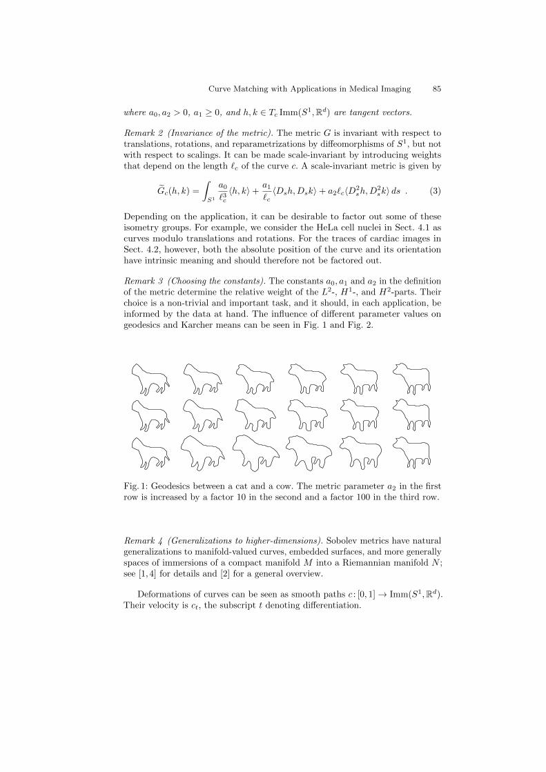
Remark 3 (Choosing the constants). The constants a0, a1 and a2 in the definitionof the metric determine the relative weight of the L2-, H1-, and H2-parts. Theirchoice is a non-trivial and important task, and it should, in each application, beinformed by the data at hand. The influence of different parameter values ongeodesics and Karcher means can be seen in Fig. 1 and Fig. 2.

Fig. 1: Geodesics between a cat and a cow. The metric parameter a2 in the firstrow is increased by a factor 10 in the second and a factor 100 in the third row.

Remark 4 (Generalizations to higher-dimensions). Sobolev metrics have naturalgeneralizations to manifold-valued curves, embedded surfaces, and more generallyspaces of immersions of a compact manifold M into a Riemannian manifold N ;see [1, 4] for details and [2] for a general overview.

Deformations of curves can be seen as smooth paths c : [0, 1]→ Imm(S1,Rd).Their velocity is ct, the subscript t denoting differentiation.


Fig. 2: Karcher means (bold) of three rotated ellipses (dashed). The parametera2 of the metric used in the first figure is increased by a factor 10 in the secondand by a factor 100 in the third figure.

Definition 5 (Geodesic distance). The length of a path of curves c is

L(c) =

∫ 1

0

√Gc(t)(ct(t), ct(t)) dt . (4)

The distance between two curves in Imm(S1,Rd) (with respect to the metric G)is the infimum of the lengths of all paths connecting these curves.

dist(c0, c1) = infc(0)=c0,c(1)=c1

L(c) .

Geodesics are locally distance-minimizing paths.

Geodesics can be described by a partial differential equation, called thegeodesic equation. It is the first order condition for minima of the energy

E(c) =1

2

∫ 1

0

Gc(t)(ct(t), ct(t)

)dt . (5)

Recently, some local and global existence results for geodesics of Sobolev metricswere shown in [7, 8, 13]. Since they provide the theoretical underpinnings for thenumerical methods presented in this paper, we summarize them here.

Theorem 6 (Geodesic equation). Let a0, a2 > 0 and a1 ≥ 0. The geodesicequation of the metric G, written in terms of the momentum p = |c′|(a0ct −a1D

2sct + a2D

4sct), is given by

∂tp =− a02|cθ|Ds(〈ct, ct〉Dsc) +

a12|cθ|Ds(〈Dsct, Dsct〉Dsc)

− a22|cθ|Ds(〈D3

sct, Dsct〉Dsc) +a22|cθ|Ds(〈D2

sct, D2sct〉Dsc) . (6)

Given any initial condition (c0, u0) ∈ T Imm(S1,R2), the solution of the geodesicequation exists for all time.

If, however, a0, a1 > 0 and a2 = 0, then G is a first order Sobolev metric. Itsgeodesic equation is locally, but not globally, well-posed.

Remark 7 (Comparison to elastic metrics). Closely related are elastic metrics [14],which in the planar case are given by

Gc(h, k) =

∫S1

a2〈Dsh, n〉〈Dsk, n〉+ b2〈Dsh, v〉〈Dsk, v〉ds . (7)


Here a, b are constants and v, n denote the unit tangent and normal vectors to c.Two special cases deserve to be highlighted: for a = 1, b = 1

2 [23] and a = b [26]there exist nonlinear transforms, the square root velocity transform and the basicmapping, that greatly simplify numerics. Both of these metrics have been appliedto a variety of problems in shape analysis.

We note that the elastic metric with a = b corresponds to a first order Sobolevmetric as in Def. 1 with a0 = a2 = 0 and a1 = a2 = b2. As it has no L2-part, itis a Riemannian metric only on the space of curves modulo translations.

3 Discretization

We propose to represent paths of curves as tensor product B-splines

c(t, θ) =

Nt∑i=1

Nθ∑j=1

ci,jBi(t)Cj(θ) (8)

of degree nt in time (t) and nθ in space (θ), respectively, using Nt and Nθ basisfunctions and controls ci,j ∈ Rd. The spatial basis functions Cj are defined onthe uniform knot sequence θj = j−n

2π·Nθ , 0 ≤ j ≤ 2n + Nθ, and satisfy periodicboundary conditions. The time basis functions Bi are defined using uniform knotson the interior of the interval [0, 1] and with full multiplicity on the boundary. Fullmultiplicity of the boundary knots ensures that fixing the initial and final curvesis equivalent to fixing the control points c1,j and cNt,j . Regarding smoothness,we have Bi ∈ Cnt−1([0, 1]) and Cj ∈ Cnθ−1([0, 2π]).

The proposed discretization scheme is independent of the special form of themetric, and can be applied equally to the scale-invariant versions as well as tothe family of elastic metrics.

3.1 Boundary Value Problem for Geodesics

To evaluate the energy (5) on discretized paths (8), we use Gaussian quadratureon each interval between subsequent knots. The resulting discretized energyEdiscr(c1,1, . . . , cNt,Nθ ) is minimized over all discrete paths (8) with fixed initialand final control points c1,j and cNt,j . This is a finite-dimensional, nonlinear,unconstrained6 optimization problem.

We solved this problem using either Matlab’s fminunc function with gradientscomputed by finite differences, or using AMPL [10] and the Ipopt solver [25]with gradients computed by automatic differentiation. By classical approximationresults [22], the discrete energy of discrete paths converges to the continuousenergy of smooth paths as the number of control points tends to infinity. Hencewe expect to obtain close approximations of geodesics. Establishing rigorousconvergence results for our discretization will be the subject of future work.

6 We neglect the condition cθ(t, θ) 6= 0. All smooth paths violating this condition haveinfinite energy because of the completeness of the metric. By approximation, splinepaths violating this condition have very high energy and will, in practice, be avoidedduring optimization.


3.2 Computing the Karcher Mean

The Karcher mean c of a set {c1, . . . , cn} of curves is the minimizer of

F (c) =1

n

n∑j=1

dist(c, cj)2 . (9)

It can be calculated by a gradient descent on (Imm(S1,Rd), G). Letting Logc cjdenote the Riemannian logarithm, the gradient of F with respect to G is [17]

gradG F (c) =1

n

n∑j=1

Logc cj . (10)

3.3 Initial Value Problem for Geodesics

To calculate the Karcher mean by gradient descent, one has to repeatedly solve thegeodesic equation (6). To this aim, we use the time-discrete variational geodesiccalculus [21]. Given three curves c0, c1, c2, one defines the discrete energy

E2(c0, c1, c2) = Gc0(c1 − c0, c1 − c0) +Gc1(c2 − c1, c2 − c1) . (11)

A 3-tuple (c0, c1, c2) is a discrete geodesic if it is a minimizer of the discreteenergy E2 with fixed endpoints c0, c2. The discrete exponential map is definedas follows: c2 = Expc0 c1, if (c0, c1, c2) is a discrete geodesic, in other words, ifc1 = argminE2(c0, ·, c2). To find c2, we differentiate the discrete energy E2 withrespect to c1 and solve the resulting system of nonlinear equations,

2Gc0(c1 − c0, ·)− 2Gc1(c2 − c1, ·) +Dc1G·(c2 − c1, c2 − c1) = 0 . (12)

We use the solver fsolve in Matlab to solve this system of equations.Given a time resolution ∆t and an initial velocity v, we choose c1 = c0 + v∆t

and compute c2 = Expc0 c1. The procedure is repeated with c1, c2 in order tocompute c3 = Expc1 c2, which is iterated until we reach the required final time.

While the convergence results in [21] do not apply to our setting, we foundgood experimental agreement with the solutions of the boundary value problem.

4 Applications

4.1 Hela Cells

In our first example we want to characterize nuclear shape variation in HeLa cells.We use fluorescence microscope images of HeLa cell nuclei7 (87 images in total).The acquisition of the cells is described in [5]. A similar study on this datasetwas performed using the LDDMM framework in [19,20]; applying intrinsically

7 The dataset was downloaded from http://murphylab.web.cmu.edu/data.


defined Sobolev metrics to the same problem will provide a complimentary pointof view.

To extract the boundary of the nucleus, we apply a thresholding method [16]to obtain a binary image and then fit – using least squares – a spline with Nθ = 12and nθ = 4 to the longest 4-connected component of the thresholded image. Thenwe reparametrize the boundary to approximately constant speed. The remainingdegree of freedom is the starting point of the parametrization; when computingminimizing geodesics, we minimize over this parameter as well. The shapes ofcell nuclei are thus represented by curves modulo translations, rotations, andconstant shifts of the parametrisation, i.e. the two curves c and eiβc(·−α)+λ areconsidered equivalent. Examples of the extracted curves are depicted in Fig. 3.

Fig. 3: Eight boundaries of HeLa cell nuclei, the Karcher mean of all nuclei(enlarged), and six randomly sampled cells using a Gaussian distribution innormal coordinates with the same covariance as the data.

The parameters a0, a1, and a2 of the Riemannian metric are chosen as follows:we compute the average L2-, H1- and H2-contributions EL2 , EH1 , EH2 to theenergy of linear paths between each pair of curves in the dataset. As the L2- andH2-contributions scale differently, we rescale all curves such that EL2 = EH2 .Then we choose constants a0, a1, and a2 such that

a0EL2 : a1EH1 : a2EH2 = 3 : 1 : 6 and E = a0EL2 + a1EH1+ a2EH2 = 100 ,

resulting in an average length `c = 12.45 and a0 = 3.36, a1 = 2.20, and a2 = 6.73.

Fig. 4: Geodesics from the mean in the first four principal directions. The curvesshow the geodesic at times −3,−2, . . . , 2, 3; the bold curve is the mean. One cansee four different characteristic deformations of the cell: bending, stretching alongthe long axis, stretching along the short axis, and a combination of stretchingwith partial bending.


The average shape of the nucleus can be captured by the Karcher mean c. Tocompute the Karcher mean of the 87 nuclei, we use a conjugate gradient methodon the Riemannian manifold of curves, as implemented in the Manopt library [6],to solve the minimization problem (9). We obtain convergence in 28 steps; thefinal value of the objective function (9) is F (c) = 10.55 and the norm of thegradient is ‖ gradG F (c)‖c < 10−3. The mean shape can be seen in Fig. 3.

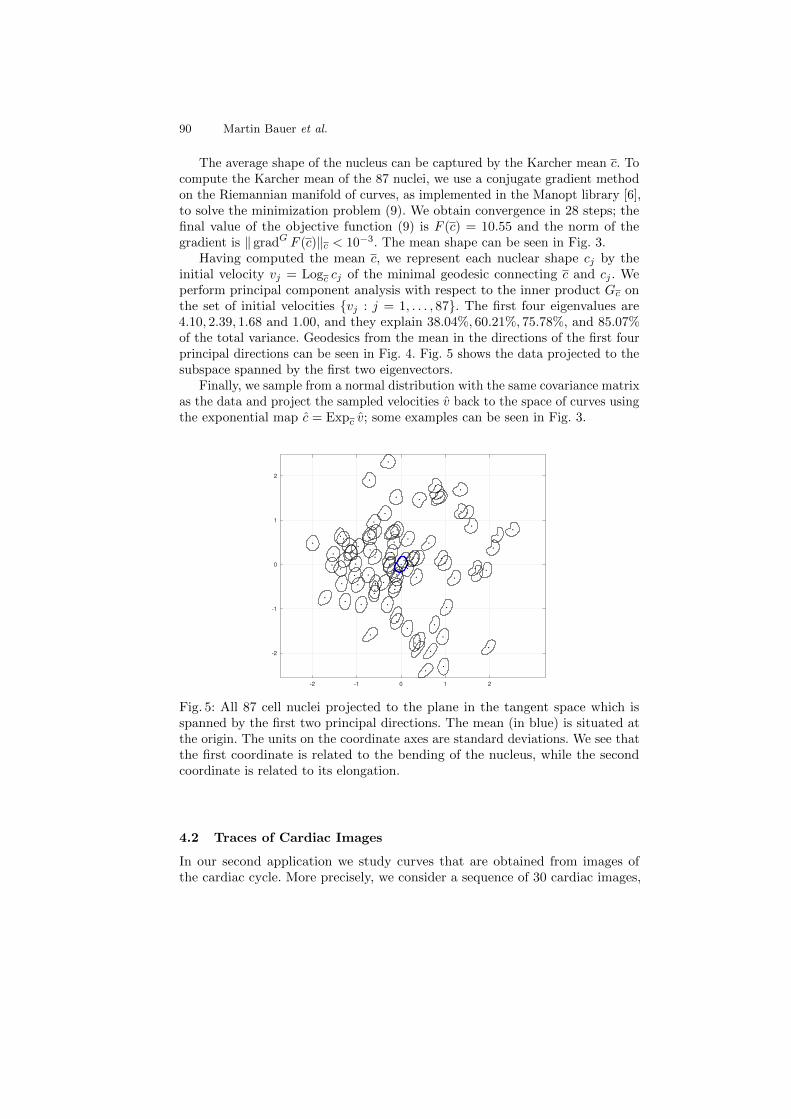
Having computed the mean c, we represent each nuclear shape cj by theinitial velocity vj = Logc cj of the minimal geodesic connecting c and cj . Weperform principal component analysis with respect to the inner product Gc onthe set of initial velocities {vj : j = 1, . . . , 87}. The first four eigenvalues are4.10, 2.39, 1.68 and 1.00, and they explain 38.04%, 60.21%, 75.78%, and 85.07%of the total variance. Geodesics from the mean in the directions of the first fourprincipal directions can be seen in Fig. 4. Fig. 5 shows the data projected to thesubspace spanned by the first two eigenvectors.

Finally, we sample from a normal distribution with the same covariance matrixas the data and project the sampled velocities v back to the space of curves usingthe exponential map c = Expc v; some examples can be seen in Fig. 3.

-2 -1 0 1 2

-2

-1

0

1

2

Fig. 5: All 87 cell nuclei projected to the plane in the tangent space which isspanned by the first two principal directions. The mean (in blue) is situated atthe origin. The units on the coordinate axes are standard deviations. We see thatthe first coordinate is related to the bending of the nucleus, while the secondcoordinate is related to its elongation.

4.2 Traces of Cardiac Images

In our second application we study curves that are obtained from images ofthe cardiac cycle. More precisely, we consider a sequence of 30 cardiac images,


taken at equispaced time points along the cardiac cycle. Each image is pro-jected to a barycentric subspace of dimension two, yielding a closed curve in thetwo-dimensional space of barycentric coordinates. After normalizing the coordi-nates [18, Sect. 3] we obtain a closed, plane curve – with the curve parameterrepresenting time – to which we can apply the methods presented in Sect. 2.Details regarding the acquisition and projection of the images can be foundin [12,24]; barycentric subspaces on manifolds are described in [18].

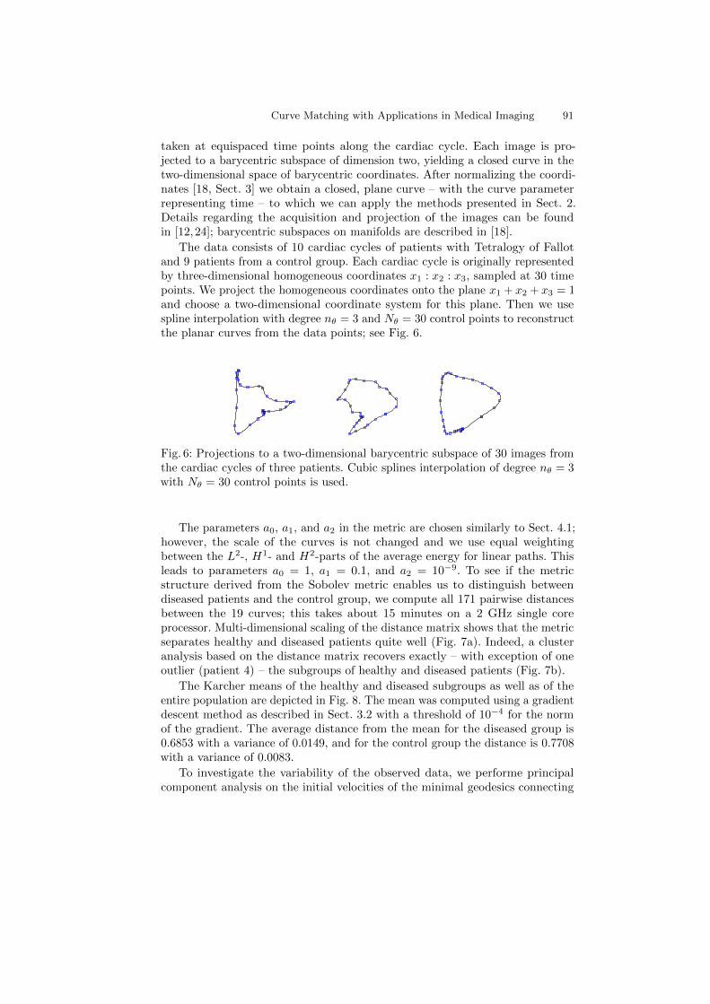
The data consists of 10 cardiac cycles of patients with Tetralogy of Fallotand 9 patients from a control group. Each cardiac cycle is originally representedby three-dimensional homogeneous coordinates x1 : x2 : x3, sampled at 30 timepoints. We project the homogeneous coordinates onto the plane x1 + x2 + x3 = 1and choose a two-dimensional coordinate system for this plane. Then we usespline interpolation with degree nθ = 3 and Nθ = 30 control points to reconstructthe planar curves from the data points; see Fig. 6.

Fig. 6: Projections to a two-dimensional barycentric subspace of 30 images fromthe cardiac cycles of three patients. Cubic splines interpolation of degree nθ = 3with Nθ = 30 control points is used.

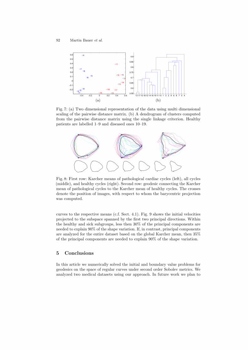
The parameters a0, a1, and a2 in the metric are chosen similarly to Sect. 4.1;however, the scale of the curves is not changed and we use equal weightingbetween the L2-, H1- and H2-parts of the average energy for linear paths. Thisleads to parameters a0 = 1, a1 = 0.1, and a2 = 10−9. To see if the metricstructure derived from the Sobolev metric enables us to distinguish betweendiseased patients and the control group, we compute all 171 pairwise distancesbetween the 19 curves; this takes about 15 minutes on a 2 GHz single coreprocessor. Multi-dimensional scaling of the distance matrix shows that the metricseparates healthy and diseased patients quite well (Fig. 7a). Indeed, a clusteranalysis based on the distance matrix recovers exactly – with exception of oneoutlier (patient 4) – the subgroups of healthy and diseased patients (Fig. 7b).

The Karcher means of the healthy and diseased subgroups as well as of theentire population are depicted in Fig. 8. The mean was computed using a gradientdescent method as described in Sect. 3.2 with a threshold of 10−4 for the normof the gradient. The average distance from the mean for the diseased group is0.6853 with a variance of 0.0149, and for the control group the distance is 0.7708with a variance of 0.0083.

To investigate the variability of the observed data, we performe principalcomponent analysis on the initial velocities of the minimal geodesics connecting


−0.4 −0.2 0 0.2 0.4 0.6

−0.2

−0.1

0

0.1

0.2

0.3

0.4

0.5

0.6

1

2 3

4

5

6

7

8

9

10

11

12

13

14

15

16

17 18

19

(a)

13 17 15 18 12 14 16 19 11 10 1 3 2 9 6 8 7 5 4

0.55

0.6

0.65

0.7

0.75

0.8

0.85

0.9

(b)

Fig. 7: (a) Two dimensional representation of the data using multi dimensionalscaling of the pairwise distance matrix. (b) A dendrogram of clusters computedfrom the pairwise distance matrix using the single linkage criterion. Healthypatients are labelled 1–9 and diseased ones 10–19.

Fig. 8: First row: Karcher means of pathological cardiac cycles (left), all cycles(middle), and healthy cycles (right). Second row: geodesic connecting the Karchermean of pathological cycles to the Karcher mean of healthy cycles. The crossesdenote the position of images, with respect to whom the barycentric projectionwas computed.

curves to the respective means (c.f. Sect. 4.1). Fig. 9 shows the initial velocitiesprojected to the subspace spanned by the first two principal directions. Withinthe healthy and sick subgroups, less then 30% of the principal components areneeded to explain 90% of the shape variation. If, in contrast, principal componentsare analyzed for the entire dataset based on the global Karcher mean, then 35%of the principal components are needed to explain 90% of the shape variation.

5 Conclusions

In this article we numerically solved the initial and boundary value problems forgeodesics on the space of regular curves under second order Sobolev metrics. Weanalyzed two medical datasets using our approach. In future work we plan to


−2 −1 0 1

−2

−1.5

−1

−0.5

0

0.5

1

1.5

10

11

12

13

14 15

16 17

18

19

S

(a)

−2 −1 0 1 2−1.5

−1

−0.5

0

0.5

1

1.5

2

2.5

1

2

3 4

5

6

7

8

9

H

(b)

−1.5 −1 −0.5 0 0.5 1 1.5

−3

−2

−1

0

1

2

1

2 3

4

5

6 7

8

9

10

11 12

13

14

15 16 17

18 19 M

(c)

Fig. 9: (a) Initial velocities of minimizing geodesics projected to the subspacespanned by first two principal components for the diseased group. (b) The samepicture for the control group. (c) The same picture for the whole population.

prove rigorous convergence results for our discretizations, further investigate theimpact of the constants in the metric, and treat unparametrized curves.

Acknowledgments

We would like to thank Xavier Pennec and Marc-Michel Rohe for providing usthe cardiac image data and Hermann Schichl for his invaluable help with AMPL.

References

1. Bauer, M., Bruveris, M.: A new Riemannian setting for surface registration. In:3nd MICCAI Workshop on Mathematical Foundations of Computational Anatomy.pp. 182–194 (2011)

2. Bauer, M., Bruveris, M., Michor, P.W.: Overview of the geometries of shape spacesand diffeomorphism groups. J. Math. Imaging Vis. 50, 60–97 (2014)

3. Bauer, M., Bruveris, M., Michor, P.W.: R-transforms for Sobolev H2-metrics onspaces of plane curves. Geom. Imaging Comput. 1(1), 1–56 (2014)

4. Bauer, M., Harms, P., Michor, P.W.: Sobolev metrics on shape space of surfaces. J.Geom. Mech. 3(4), 389–438 (2011)

5. Boland, M.V., Murphy, R.F.: A neural network classifier capable of recognizing thepatterns of all major subcellular structures in fluorescence microscope images ofHeLa cells. Bioinformatics 17(12), 1213–1223 (2001)

6. Boumal, N., Mishra, B., Absil, P.A., Sepulchre, R.: Manopt, a Matlab toolbox foroptimization on manifolds. J. Mach. Learn. Res. 15, 1455–1459 (2014)

7. Bruveris, M.: Completeness properties of Sobolev metrics on the space of curves. J.Geom. Mech. 7(2) (2015)

8. Bruveris, M., Michor, P.W., Mumford, D.: Geodesic completeness for Sobolevmetrics on the space of immersed plane curves. Forum Math. Sigma 2, e19 (2014)

9. Dryden, I.L., Mardia, K.V.: Statistical Shape Analysis. Wiley Series in Probabilityand Statistics, John Wiley & Sons, Ltd., Chichester (1998)


10. Fourer, R., Gay, D., Kernighan, B.W.: The AMPL book (2002)11. Krim, H., Yezzi, Jr., A. (eds.): Statistics and Analysis of Shapes. Modeling and

Simulation in Science, Engineering and Technology, Birkhauser Boston (2006)12. McLeod, K., Sermesant, M., Beerbaum, P., Pennec, X.: Spatio-temporal tensor

decomposition of a polyaffine motion model for a better analysis of pathologicalleft ventricular dynamics. IEEE Trans. Med. Imaging (2015)

13. Michor, P.W., Mumford, D.: An overview of the Riemannian metrics on spacesof curves using the Hamiltonian approach. Appl. Comput. Harmon. Anal. 23(1),74–113 (2007)

14. Mio, W., Srivastava, A., Joshi, S.: On shape of plane elastic curves. Int. J. Comput.Vision 73(3), 307–324 (Jul 2007)

15. Nardi, G., Peyre, G., Vialard, F.X.: Geodesics on shape spaces with boundedvariation and Sobolev metrics. http://arxiv.org/abs/1402.6504 (2014)

16. Otsu, N.: A threshold selection method from gray-level histograms. IEEE T. Syst.Man Cyb. 9(1), 62–66 (1979)

17. Pennec, X.: Intrinsic statistics on Riemannian manifolds: basic tools for geometricmeasurements. J. Math. Imaging Vision 25(1), 127–154 (2006)

18. Pennec, X.: Barycentric subspaces and affine spans in manifolds (2015), to appearin the proceeding of Geometric Science of Information, 2015

19. Rohde, G.K., Ribeiro, A.J.S., Dahl, K.N., Murphy, R.F.: Deformation-based nuclearmorphometry: capturing nuclear shape variation in HeLa cells. Cytometry Part A73A(4), 341–350 (2008)

20. Rohde, G.K., Wang, W., Peng, T., Murphy, R.F.: Deformation-based nonlineardimension reduction: applications to nuclear morphometry. In: 5th IEEE Int. Sym-posium on Biomedical Imaging: From Nano to Macro. pp. 500–503 (2008)

21. Rumpf, M., Wirth, B.: Variational time discretization of geodesic calculus. IMAJournal of Numerical Analysis (2014)

22. Schumaker, L.L.: Spline Functions: Basic Theory. Cambridge Mathematical Library,Cambridge University Press, Cambridge, third edn. (2007)

23. Srivastava, A., Klassen, E., Joshi, S.H., Jermyn, I.H.: Shape analysis of elasticcurves in Euclidean spaces. IEEE T. Pattern Anal. 33(7), 1415–1428 (2011)

24. Tobon-Gomez, C., De Craene, M., Mcleod, K., Tautz, L., Shi, W., Hennemuth,A., Prakosa, A., Wang, H., Carr-White, G., Kapetanakis, S., Lutz, A., Rasche, V.,Schaeffter, T., Butakoff, C., Friman, O., Mansi, T., Sermesant, M., Zhuang, X.,Ourselin, S., Peitgen, H.O., Pennec, X., Razavi, R., Rueckert, D., Frangi, A.F.,Rhode, K.: Benchmarking framework for myocardial tracking and deformationalgorithms: an open access database. Medical Image Analysis 17(6), 632–648 (2013)

25. Wachter, A., Biegler, L.T.: On the implementation of an interior-point filter line-search algorithm for large-scale nonlinear programming. Math. Program. 106(1),25–57 (2006)

26. Younes, L., Michor, P.W., Shah, J., Mumford, D.: A metric on shape space withexplicit geodesics. Atti Accad. Naz. Lincei Cl. Sci. Fis. Mat. Natur. Rend. Lincei(9) Mat. Appl. 19(1), 25–57 (2008)

27. Younes, L.: Spaces and manifolds of shapes in computer vision: an overview. ImageVision Comput. 30(6), 389–397 (2012)

curve matching with applications in medical imaging · curve matching with applications in medical...

Documents