curveexpert basic...
TRANSCRIPT
CurveExpert Basic DocumentationRelease 2.1.0
Daniel G. Hyams
Nov 23, 2017

CONTENTS
1 What is CurveExpert Basic? 1
2 Installation and Activation 32.1 Installation . . . . . . . . . . . . . . . . . . . . . . . . . . . . . . . . . . . . . . . . . . . . . . . . 32.2 Starting a Trial . . . . . . . . . . . . . . . . . . . . . . . . . . . . . . . . . . . . . . . . . . . . . . 32.3 Purchasing . . . . . . . . . . . . . . . . . . . . . . . . . . . . . . . . . . . . . . . . . . . . . . . . 42.4 After Purchase: licensing . . . . . . . . . . . . . . . . . . . . . . . . . . . . . . . . . . . . . . . . 42.5 Automated licensing . . . . . . . . . . . . . . . . . . . . . . . . . . . . . . . . . . . . . . . . . . . 4
3 Getting started 53.1 Load data into CurveExpert Basic . . . . . . . . . . . . . . . . . . . . . . . . . . . . . . . . . . . . 63.2 Perform a Nonlinear Regression . . . . . . . . . . . . . . . . . . . . . . . . . . . . . . . . . . . . . 63.3 Examine the Results . . . . . . . . . . . . . . . . . . . . . . . . . . . . . . . . . . . . . . . . . . . 63.4 Visualize your Results . . . . . . . . . . . . . . . . . . . . . . . . . . . . . . . . . . . . . . . . . . 6
4 User Interface 74.1 Menus . . . . . . . . . . . . . . . . . . . . . . . . . . . . . . . . . . . . . . . . . . . . . . . . . . 84.2 Toolbar . . . . . . . . . . . . . . . . . . . . . . . . . . . . . . . . . . . . . . . . . . . . . . . . . . 94.3 Results Pane . . . . . . . . . . . . . . . . . . . . . . . . . . . . . . . . . . . . . . . . . . . . . . . 104.4 Graphs and Data Pane . . . . . . . . . . . . . . . . . . . . . . . . . . . . . . . . . . . . . . . . . . 114.5 Preview Pane . . . . . . . . . . . . . . . . . . . . . . . . . . . . . . . . . . . . . . . . . . . . . . . 114.6 Messages Pane . . . . . . . . . . . . . . . . . . . . . . . . . . . . . . . . . . . . . . . . . . . . . . 114.7 Status bar . . . . . . . . . . . . . . . . . . . . . . . . . . . . . . . . . . . . . . . . . . . . . . . . . 114.8 Menu Reference . . . . . . . . . . . . . . . . . . . . . . . . . . . . . . . . . . . . . . . . . . . . . 12
5 Reading Data 155.1 Introduction . . . . . . . . . . . . . . . . . . . . . . . . . . . . . . . . . . . . . . . . . . . . . . . 155.2 Raw file import . . . . . . . . . . . . . . . . . . . . . . . . . . . . . . . . . . . . . . . . . . . . . . 155.3 CurveExpert Basic files . . . . . . . . . . . . . . . . . . . . . . . . . . . . . . . . . . . . . . . . . 18
6 Working with Data 216.1 Introduction . . . . . . . . . . . . . . . . . . . . . . . . . . . . . . . . . . . . . . . . . . . . . . . 216.2 Data statistics . . . . . . . . . . . . . . . . . . . . . . . . . . . . . . . . . . . . . . . . . . . . . . . 216.3 The spreadsheet . . . . . . . . . . . . . . . . . . . . . . . . . . . . . . . . . . . . . . . . . . . . . 216.4 Number Formatting . . . . . . . . . . . . . . . . . . . . . . . . . . . . . . . . . . . . . . . . . . . 236.5 Operating on Data . . . . . . . . . . . . . . . . . . . . . . . . . . . . . . . . . . . . . . . . . . . . 24
7 Calculating Results 277.1 General Guidelines . . . . . . . . . . . . . . . . . . . . . . . . . . . . . . . . . . . . . . . . . . . . 277.2 Interpolation . . . . . . . . . . . . . . . . . . . . . . . . . . . . . . . . . . . . . . . . . . . . . . . 287.3 Linear Regression . . . . . . . . . . . . . . . . . . . . . . . . . . . . . . . . . . . . . . . . . . . . 29
i
7.4 Nonlinear Regression . . . . . . . . . . . . . . . . . . . . . . . . . . . . . . . . . . . . . . . . . . 29
8 CurveFinder 338.1 Usage . . . . . . . . . . . . . . . . . . . . . . . . . . . . . . . . . . . . . . . . . . . . . . . . . . . 338.2 Cautions . . . . . . . . . . . . . . . . . . . . . . . . . . . . . . . . . . . . . . . . . . . . . . . . . 33
9 Working with Results 359.1 Introduction . . . . . . . . . . . . . . . . . . . . . . . . . . . . . . . . . . . . . . . . . . . . . . . 359.2 Color Coding . . . . . . . . . . . . . . . . . . . . . . . . . . . . . . . . . . . . . . . . . . . . . . . 359.3 Badges . . . . . . . . . . . . . . . . . . . . . . . . . . . . . . . . . . . . . . . . . . . . . . . . . . 369.4 Previewing . . . . . . . . . . . . . . . . . . . . . . . . . . . . . . . . . . . . . . . . . . . . . . . . 379.5 Placing Results on a Graph . . . . . . . . . . . . . . . . . . . . . . . . . . . . . . . . . . . . . . . . 379.6 Removing Results . . . . . . . . . . . . . . . . . . . . . . . . . . . . . . . . . . . . . . . . . . . . 379.7 Copying Result Information . . . . . . . . . . . . . . . . . . . . . . . . . . . . . . . . . . . . . . . 379.8 Querying Result Details . . . . . . . . . . . . . . . . . . . . . . . . . . . . . . . . . . . . . . . . . 379.9 Confidence and Prediction Bands . . . . . . . . . . . . . . . . . . . . . . . . . . . . . . . . . . . . 38
10 Graphing 4110.1 Introduction . . . . . . . . . . . . . . . . . . . . . . . . . . . . . . . . . . . . . . . . . . . . . . . 4110.2 Graph Types . . . . . . . . . . . . . . . . . . . . . . . . . . . . . . . . . . . . . . . . . . . . . . . 4110.3 Basics . . . . . . . . . . . . . . . . . . . . . . . . . . . . . . . . . . . . . . . . . . . . . . . . . . . 4110.4 Interacting with a graph . . . . . . . . . . . . . . . . . . . . . . . . . . . . . . . . . . . . . . . . . 4210.5 Changing Graph Properties . . . . . . . . . . . . . . . . . . . . . . . . . . . . . . . . . . . . . . . 4510.6 Legend . . . . . . . . . . . . . . . . . . . . . . . . . . . . . . . . . . . . . . . . . . . . . . . . . . 5010.7 Saving graphs . . . . . . . . . . . . . . . . . . . . . . . . . . . . . . . . . . . . . . . . . . . . . . 5110.8 Copying graphs . . . . . . . . . . . . . . . . . . . . . . . . . . . . . . . . . . . . . . . . . . . . . . 5210.9 Printing graphs . . . . . . . . . . . . . . . . . . . . . . . . . . . . . . . . . . . . . . . . . . . . . . 5210.10 Keyboard Shortcuts for Graphs . . . . . . . . . . . . . . . . . . . . . . . . . . . . . . . . . . . . . 5210.11 Mathtext . . . . . . . . . . . . . . . . . . . . . . . . . . . . . . . . . . . . . . . . . . . . . . . . . 52
11 Creating Custom Models 6111.1 Introduction . . . . . . . . . . . . . . . . . . . . . . . . . . . . . . . . . . . . . . . . . . . . . . . 6111.2 Custom Models . . . . . . . . . . . . . . . . . . . . . . . . . . . . . . . . . . . . . . . . . . . . . . 61
12 Equation Display 63
13 Writing Data 6513.1 Introduction . . . . . . . . . . . . . . . . . . . . . . . . . . . . . . . . . . . . . . . . . . . . . . . 6513.2 Writing a CurveExpert (CXP) file . . . . . . . . . . . . . . . . . . . . . . . . . . . . . . . . . . . . 6513.3 Exporting a dataset to text file . . . . . . . . . . . . . . . . . . . . . . . . . . . . . . . . . . . . . . 6513.4 Writing a graph to a picture file . . . . . . . . . . . . . . . . . . . . . . . . . . . . . . . . . . . . . 6513.5 Printing . . . . . . . . . . . . . . . . . . . . . . . . . . . . . . . . . . . . . . . . . . . . . . . . . . 65
14 Application Preferences 6714.1 Introduction . . . . . . . . . . . . . . . . . . . . . . . . . . . . . . . . . . . . . . . . . . . . . . . 6714.2 General Preferences . . . . . . . . . . . . . . . . . . . . . . . . . . . . . . . . . . . . . . . . . . . 6714.3 Regression Preferences . . . . . . . . . . . . . . . . . . . . . . . . . . . . . . . . . . . . . . . . . . 7014.4 Graphing Preferences . . . . . . . . . . . . . . . . . . . . . . . . . . . . . . . . . . . . . . . . . . 7114.5 Logging Preferences . . . . . . . . . . . . . . . . . . . . . . . . . . . . . . . . . . . . . . . . . . . 7314.6 Localization Preferences . . . . . . . . . . . . . . . . . . . . . . . . . . . . . . . . . . . . . . . . . 7414.7 Advanced Preferences . . . . . . . . . . . . . . . . . . . . . . . . . . . . . . . . . . . . . . . . . . 75
15 Localization 7715.1 Executive Summary . . . . . . . . . . . . . . . . . . . . . . . . . . . . . . . . . . . . . . . . . . . 7715.2 Configuring CurveExpert Basic to match your workflow . . . . . . . . . . . . . . . . . . . . . . . . 77
ii
15.3 File overrides . . . . . . . . . . . . . . . . . . . . . . . . . . . . . . . . . . . . . . . . . . . . . . . 7815.4 CurveExpert Basic files . . . . . . . . . . . . . . . . . . . . . . . . . . . . . . . . . . . . . . . . . 7815.5 NIST verification files . . . . . . . . . . . . . . . . . . . . . . . . . . . . . . . . . . . . . . . . . . 78
16 Validation 8116.1 Introduction . . . . . . . . . . . . . . . . . . . . . . . . . . . . . . . . . . . . . . . . . . . . . . . 8116.2 Running the Suite . . . . . . . . . . . . . . . . . . . . . . . . . . . . . . . . . . . . . . . . . . . . 8116.3 Performing validations yourself . . . . . . . . . . . . . . . . . . . . . . . . . . . . . . . . . . . . . 81
17 Miscellaneous 8317.1 Log Viewer . . . . . . . . . . . . . . . . . . . . . . . . . . . . . . . . . . . . . . . . . . . . . . . . 8317.2 Running Multiple Instances . . . . . . . . . . . . . . . . . . . . . . . . . . . . . . . . . . . . . . . 8417.3 Where files are located . . . . . . . . . . . . . . . . . . . . . . . . . . . . . . . . . . . . . . . . . . 84
18 End User License Agreement 85
19 Third-Party Licensing 8719.1 Python . . . . . . . . . . . . . . . . . . . . . . . . . . . . . . . . . . . . . . . . . . . . . . . . . . 8719.2 WxWidgets and WxPython . . . . . . . . . . . . . . . . . . . . . . . . . . . . . . . . . . . . . . . 8819.3 Numpy . . . . . . . . . . . . . . . . . . . . . . . . . . . . . . . . . . . . . . . . . . . . . . . . . . 8919.4 Scipy . . . . . . . . . . . . . . . . . . . . . . . . . . . . . . . . . . . . . . . . . . . . . . . . . . . 8919.5 Matplotlib . . . . . . . . . . . . . . . . . . . . . . . . . . . . . . . . . . . . . . . . . . . . . . . . 9019.6 xlrd . . . . . . . . . . . . . . . . . . . . . . . . . . . . . . . . . . . . . . . . . . . . . . . . . . . . 9119.7 BioPython . . . . . . . . . . . . . . . . . . . . . . . . . . . . . . . . . . . . . . . . . . . . . . . . 9219.8 winpaths . . . . . . . . . . . . . . . . . . . . . . . . . . . . . . . . . . . . . . . . . . . . . . . . . 9219.9 Python Imaging Library (PIL) . . . . . . . . . . . . . . . . . . . . . . . . . . . . . . . . . . . . . . 9219.10 Icons and Artwork . . . . . . . . . . . . . . . . . . . . . . . . . . . . . . . . . . . . . . . . . . . . 9319.11 JPEG library . . . . . . . . . . . . . . . . . . . . . . . . . . . . . . . . . . . . . . . . . . . . . . . 93
20 Appendix A: Math Functions 9520.1 Constants . . . . . . . . . . . . . . . . . . . . . . . . . . . . . . . . . . . . . . . . . . . . . . . . . 9520.2 Transcendental Functions . . . . . . . . . . . . . . . . . . . . . . . . . . . . . . . . . . . . . . . . 9520.3 Bessel Functions . . . . . . . . . . . . . . . . . . . . . . . . . . . . . . . . . . . . . . . . . . . . . 9820.4 Comparison Functions . . . . . . . . . . . . . . . . . . . . . . . . . . . . . . . . . . . . . . . . . . 10020.5 Miscellaneous Functions . . . . . . . . . . . . . . . . . . . . . . . . . . . . . . . . . . . . . . . . . 10020.6 Array Specific Functions . . . . . . . . . . . . . . . . . . . . . . . . . . . . . . . . . . . . . . . . . 10220.7 Logical Functions . . . . . . . . . . . . . . . . . . . . . . . . . . . . . . . . . . . . . . . . . . . . 106
21 Appendix B: Math Symbol Reference 10921.1 Subscripts and superscripts . . . . . . . . . . . . . . . . . . . . . . . . . . . . . . . . . . . . . . . . 10921.2 Fractions, binomials and stacked numbers . . . . . . . . . . . . . . . . . . . . . . . . . . . . . . . . 10921.3 Using parenthesis properly . . . . . . . . . . . . . . . . . . . . . . . . . . . . . . . . . . . . . . . . 10921.4 Radicals . . . . . . . . . . . . . . . . . . . . . . . . . . . . . . . . . . . . . . . . . . . . . . . . . 11021.5 Accents . . . . . . . . . . . . . . . . . . . . . . . . . . . . . . . . . . . . . . . . . . . . . . . . . . 11021.6 Symbols . . . . . . . . . . . . . . . . . . . . . . . . . . . . . . . . . . . . . . . . . . . . . . . . . 110
22 Appendix C: Theory 11522.1 Linear Regression . . . . . . . . . . . . . . . . . . . . . . . . . . . . . . . . . . . . . . . . . . . . 11522.2 Nonlinear Regression . . . . . . . . . . . . . . . . . . . . . . . . . . . . . . . . . . . . . . . . . . 115
23 Appendix D: References 119
24 Indices and tables 121
Index 123
iii

iv
CHAPTER
ONE
WHAT IS CURVEEXPERT BASIC?
CurveExpert Basic is a solution for curve fitting and data analysis for Windows. Data can be modelled using atoolbox of linear regression models and nonlinear regression models, and visualized with the built-in publicationquality graphics engine.
Over 60 models are built-in, but custom regression models may also be defined by the user. Publication-qualitygraphing capability allows thorough examination and presentation of the curve fit. The process of finding the bestfit can be automated by letting CurveExpert Basic compare your data to each model to choose the best curve. Thesoftware is designed with the purpose of generating high quality results and output while saving your time in theprocess.
CurveExpert Basic is a subset of the functionality contained in CurveExpert Professional and is intended for morecasual/infrequent users. The major features of the software are enumerated below:
• Easy-to-use User Interface: most mathematically-intensive applications are very difficult to use. CurveEx-pert Basic has a very intuitive interface, which allows you to import your data, generate results, and createpublication-quality plots with very minimal effort. In fact, to import a file takes only four clicks, and generatinga battery of results with associated graphs takes two more.
• Robust file import: data files come in many shapes and sizes, and CurveExpert Basic makes importing yourdata files very easy. The smart file reader avoids non-data areas of your file dynamically, and attempts to findlabels for each column of data in your file.
• Publication quality graphs: The rendering of the plots is of publication quality, with full antialiasing supportand the ability to customize each graph. Graphs can be saved to a variety of graphics file formats, and theymay be directly copied and pasted into another application. Graphs are interactive, with zooming, panning, andautoscaling.
• Built-in models: over 60 built-in nonlinear models, with high-quality automatic initial guesses, are availablefor use. The provided models cover all of the major families.
• Custom models: you can also define models yourself, using a very large library of built-in mathematical func-tions, and parameters in your models can take any name that you like.
• Ranking of results: results are automatically ranked by your choice of score, correlation coefficient, standarderror, or coefficient of determination.
• Validated: validated against the Statistical Reference Datasets Project of the National Institute of Standardsand Technology. These datasets can be downloaded directly at http://www.itl.nist.gov/div898/strd/general/dataarchive.html, but are also included verbatim in the CurveExpert Basic distribution for you to use yourself.
• Quality spreadsheet: the built-in spreadsheet allows you to manually enter data and/or modify it with a suiteof data transformation tools. Data entry and cutting and pasting capabilities are as easy as Excel.
• Localization: Importing data or interoperating in European-style environments (which use a comma as a dec-imal) is extremely easy; regional settings are automatically obeyed, or can be selectively enabled in order tomatch your particular workflow.
1

CurveExpert Basic Documentation, Release 2.1.0
• Logging: a log of actions is kept across sessions of the software, in case you need to recreate a particular result.A messages pane keeps you informed of the status of every computed result.
• Documentation: Extensive documentation in HTML and PDF format, available both directly from the softwareand online at http://docs.curveexpert.net/curveexpert/basic.
2 Chapter 1. What is CurveExpert Basic?

CHAPTER
TWO
INSTALLATION AND ACTIVATION
2.1 Installation
2.1.1 Windows
To install on Windows platforms, simply run the installer, either from the command line or by double clicking it in theWindows explorer. The automated installer will start and guide you through the installation process; just follow theon-screen prompts. CurveExpert Basic will install for all users (if you are the Administrator), or for you only (if youare not). This allows you to install CurveExpert Basic without any Administrator privileges.
Windows automated installs
The installer for Windows operating systems recognizes two command line switches: /S for silent installs, and/D=dirname to specify where the program should be installed. For example, in an environment where a systemadministrator would want to install the program silently to the directory “d:\sharedprogs”, one would do:
> CurveExpertBasic-2.0.0-win64.exe /S /D=d:\sharedprogs
Windows automated uninstalls
The uninstaller for Windows operating systems can be used for silent uninstalls. If the software was installed in thedirectory “c:\sharedprogs”, one would do:
> "c:\sharedprogs\CurveExpert Basic\uninstall" /S
Note that there are no quotes used in the last _? option, even if there are spaces in the path.
2.2 Starting a Trial
If you want to evaluate CurveExpert Basic on a trial basis, you can start a trial period by selecting Help->ActivateTrial Period; note that an Internet connection is required for the starting of the trial period, but is not required once thetrial period has been activated.
Note: If you use an authenticating proxy for Internet access, please set the appropriate proxy settings in Edit->Preferences->Advanced (see Proxy settings).
3
CurveExpert Basic Documentation, Release 2.1.0
This trial period is active for approximately 30 days from activation date. During this period, all features of CurveEx-pert Basic are accessible. When the software is out of its trial period (either before or after), most output functions aredisabled, and a watermark appears on all graphs.
After evaluation via the trial period, please consider purchasing the software at http://www.curveexpert.net/order.
2.3 Purchasing
To purchase CurveExpert Basic, visit http://www.curveexpert.net/order, and choose the product that you would like topurchase.
2.4 After Purchase: licensing
If you have purchased a CurveExpert Basic license, you will receive the license information via email. Licenses arefulfilled within 24 hours of receipt; average turnaround time between purchase and license fulfillment is 2 hours.
Proceed to Help->Enter License, and paste the entire email into the box. The fields below the box (Name, Company,etc.) will update, and you can then press OK to complete the process.
If you are not sure how to copy and paste the email, highlight the text of the email with your mouse (click and drag),and press Ctrl+C (Cmd+C on a Macintosh). Then, just press the Paste button in the Help->Enter License window.
Thank you for your support of CurveExpert Basic!
2.5 Automated licensing
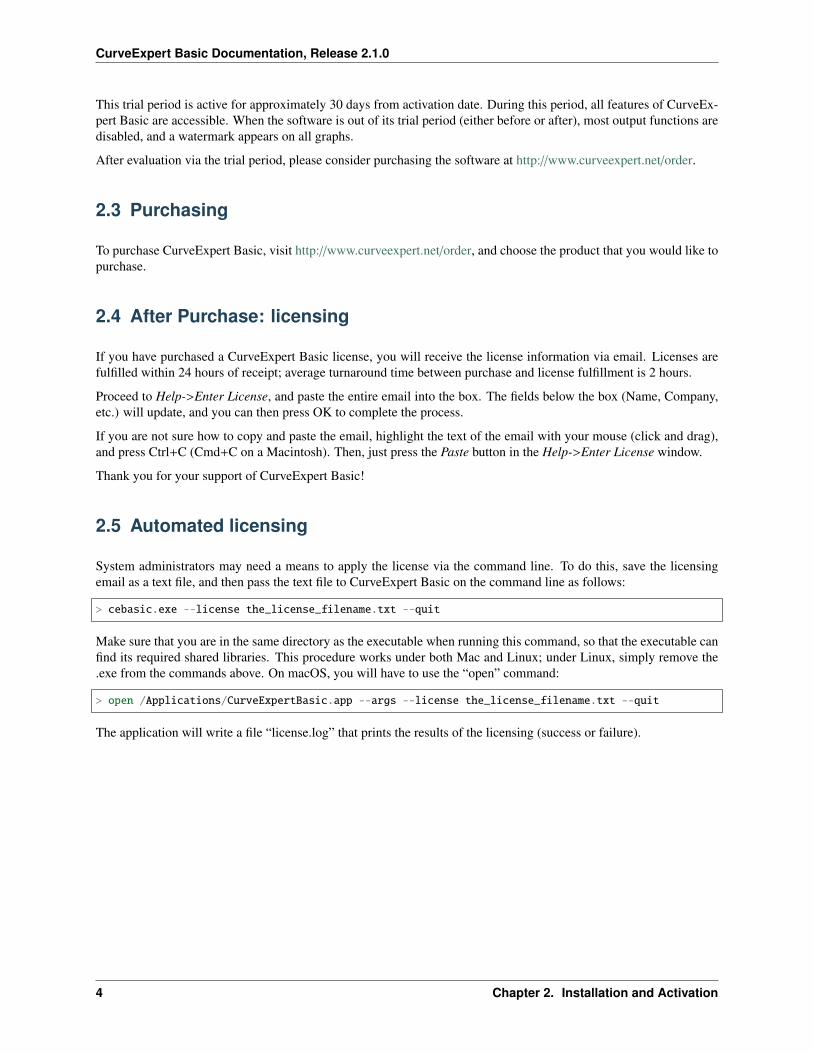
System administrators may need a means to apply the license via the command line. To do this, save the licensingemail as a text file, and then pass the text file to CurveExpert Basic on the command line as follows:
> cebasic.exe --license the_license_filename.txt --quit
Make sure that you are in the same directory as the executable when running this command, so that the executable canfind its required shared libraries. This procedure works under both Mac and Linux; under Linux, simply remove the.exe from the commands above. On macOS, you will have to use the “open” command:
> open /Applications/CurveExpertBasic.app --args --license the_license_filename.txt --quit
The application will write a file “license.log” that prints the results of the licensing (success or failure).
4 Chapter 2. Installation and Activation
CHAPTER
THREE
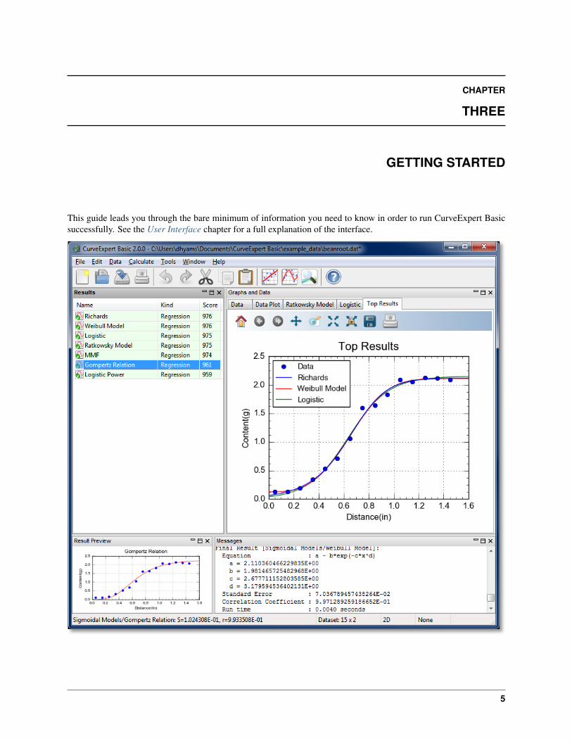
GETTING STARTED
This guide leads you through the bare minimum of information you need to know in order to run CurveExpert Basicsuccessfully. See the User Interface chapter for a full explanation of the interface.
5
CurveExpert Basic Documentation, Release 2.1.0
3.1 Load data into CurveExpert Basic
Read a sample file supplied with CurveExpert Basic. Choose File->Open, double click on “example_data”, set the filefilter to *.dat, and double click the file “beanroot.dat”. When the File Import dialog appears, simply click OK. (seeReading Data)
3.2 Perform a Nonlinear Regression
Choose Calculate->Nonlinear Model Fit. Select the Sigmoidal Models, which automatically selects all of the membersof that model family for computation. Click OK. (see Calculating Results)
3.3 Examine the Results
As a result of the computation, the results will be shown in the left pane in CurveExpert Basic, ranked in order fromthe best fit to the worst fit (see Working with Results). Double click, or right-click and select Details..., on any of theresults to see details (see Querying Result Details). Also, you can click the tabs in the graph stack (the right hand panein the application window) to see visualizations of the results. Later, you can add graphs of your own.
3.4 Visualize your Results
In the “Graphs and Data” pane, two graphs have been automatically created for you; one that shows the data only, andone that shows the data plotted with the top few results that have been computed. You can visualize any one of theresults in the “Results” pane by right clicking one (or some) of them and selecting “Send to New Plot”.
6 Chapter 3. Getting started

CHAPTER
FOUR
USER INTERFACE
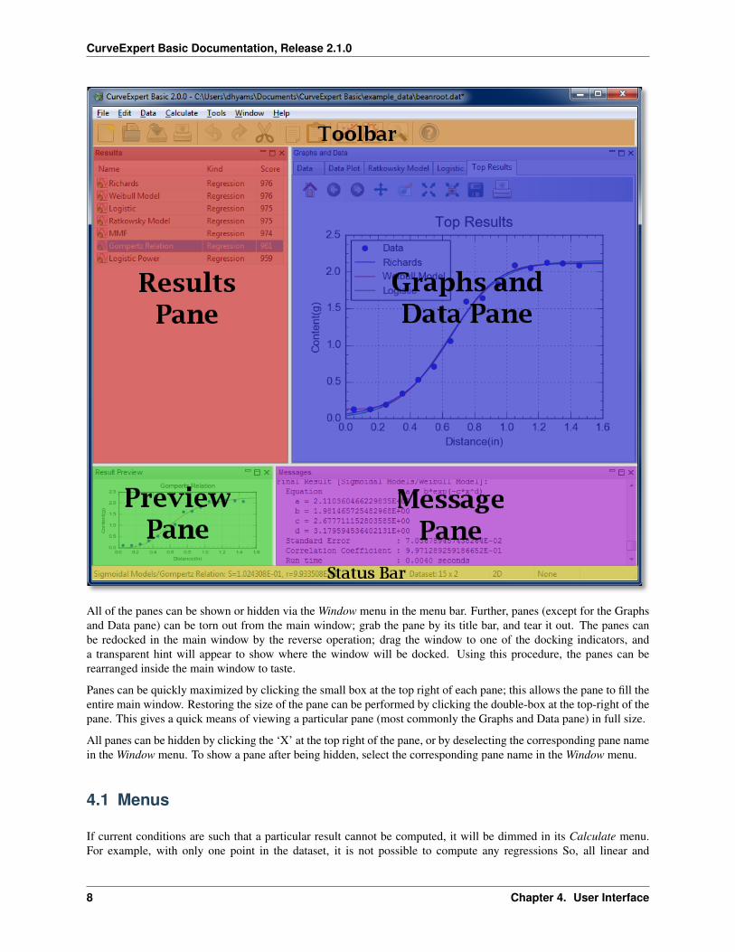
The CurveExpert Basic user interface is divided into panes:
• Results
• Graphs and Data
• Preview
• Messages
The panes, as well as the toolbar and status bar, are labeled in the graphic below:
7
CurveExpert Basic Documentation, Release 2.1.0
All of the panes can be shown or hidden via the Window menu in the menu bar. Further, panes (except for the Graphsand Data pane) can be torn out from the main window; grab the pane by its title bar, and tear it out. The panes canbe redocked in the main window by the reverse operation; drag the window to one of the docking indicators, anda transparent hint will appear to show where the window will be docked. Using this procedure, the panes can berearranged inside the main window to taste.
Panes can be quickly maximized by clicking the small box at the top right of each pane; this allows the pane to fill theentire main window. Restoring the size of the pane can be performed by clicking the double-box at the top-right of thepane. This gives a quick means of viewing a particular pane (most commonly the Graphs and Data pane) in full size.
All panes can be hidden by clicking the ‘X’ at the top right of the pane, or by deselecting the corresponding pane namein the Window menu. To show a pane after being hidden, select the corresponding pane name in the Window menu.
4.1 Menus
If current conditions are such that a particular result cannot be computed, it will be dimmed in its Calculate menu.For example, with only one point in the dataset, it is not possible to compute any regressions So, all linear and
8 Chapter 4. User Interface

CurveExpert Basic Documentation, Release 2.1.0
nonlinear regressions in the Calculate menu will be dimmed and therefore unselectable. See Menu Reference for aquick explanation of each of the menu choices.
4.2 Toolbar
The toolbar can be shown or hidden via “Window->Toolbar”.
Each button on the toolbar has a one-to-one mapping to an item in the menus. The toolbar is divided up into thefollowing sections:
• File
• Edit
• Calculate
• Tools
• Help
The buttons are each documented below.
4.2. Toolbar 9
CurveExpert Basic Documentation, Release 2.1.0
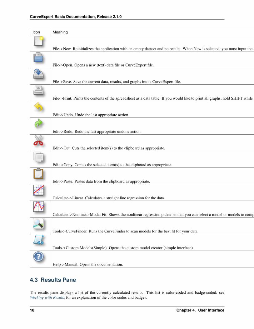
Icon Meaning
File->New. Reinitializes the application with an empty dataset and no results. When New is selected, you must input the desired number of columns in the new dataset.
File->Open. Opens a new (text) data file or CurveExpert file.
File->Save. Save the current data, results, and graphs into a CurveExpert file.
File->Print. Prints the contents of the spreadsheet as a data table. If you would like to print all graphs, hold SHIFT while selecting File->Print.
Edit->Undo. Undo the last appropriate action.
Edit->Redo. Redo the last appropriate undone action.
Edit->Cut. Cuts the selected item(s) to the clipboard as appropriate.
Edit->Copy. Copies the selected item(s) to the clipboard as appropriate.
Edit->Paste. Pastes data from the clipboard as appropriate.
Calculate->Linear. Calculates a straight line regression for the data.
Calculate->Nonlinear Model Fit. Shows the nonlinear regression picker so that you can select a model or models to compute.
Tools->CurveFinder. Runs the CurveFinder to scan models for the best fit for your data
Tools->Custom Models(Simple). Opens the custom model creator (simple interface)
Help->Manual. Opens the documentation.
4.3 Results Pane
The results pane displays a list of the currently calculated results. This list is color-coded and badge-coded; seeWorking with Results for an explanation of the color codes and badges.
10 Chapter 4. User Interface
CurveExpert Basic Documentation, Release 2.1.0
The items displayed in the columns of the results pane can be customized by right-clicking the column headers. Thefollowing items may be selected for display:
• Name (required; cannot be deactivated)
• Kind
• Family
• Score
• R (correlation coefficient)
• R^2 (coefficient of determination)
• Std_Err (standard error)
Remember that you can send results to a plot, remove a result, or view result details by right-clicking a particularresult. See Working with Results for details.
4.4 Graphs and Data Pane
The “Graphs and Data” pane is a notebook where the dataset and graphs reside. Please refer to The spreadsheetfor information on how to work with the dataset via the built-in spreadsheet. Refer to Graphing for documentationconcerning how to work with graphs.
4.5 Preview Pane
The preview pane displays the result that is pointed to in the Result pane, or, if a result is pointed to in a graph, thepreview pane also updates to the pointed-to-result. While convenient, the preview window can cause the user interfaceto be sluggish on older computers; to disable the preview, simply hide it by deselecting Window->Preview, or morestraightforwardly, click the ‘X’ at the top right of the preview pane.
4.6 Messages Pane
The Messages Pane is an area where CurveExpert Basic sends all notifications for your perusal. For example, when afile is read, the a summary of the file contents appears in the Messages pane. Also, when any calculation is undertaken,a summary of the result appears in the Messages pane.
The content of the messages pane can be copied and pasted to another application by highlighting a portion, right-clicking, and selecting Copy, or by using Ctrl+C.
Error messages appear in the Messages pane in red, and special messages appear in blue. All messages that appear inthe Message pane are automatically logged, and be accessed after-the-fact via Tools->Log Viewer (see Log Viewer).
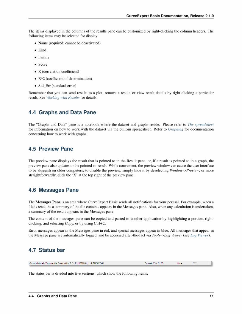
4.7 Status bar
The status bar is divided into five sections, which show the following items:
4.4. Graphs and Data Pane 11
CurveExpert Basic Documentation, Release 2.1.0
Sec-tion
Displays
1 typically shows vital statistics for the currently pointed-to result, or displays help when appropriate.2 size of the currrent dataset (nrows x ncolumns)3 dimension of the dataset, which determines the mode of the application4 current locale5 number of helper processes present that perform calculations (see multicore). Each asterisk represents
one helper process.
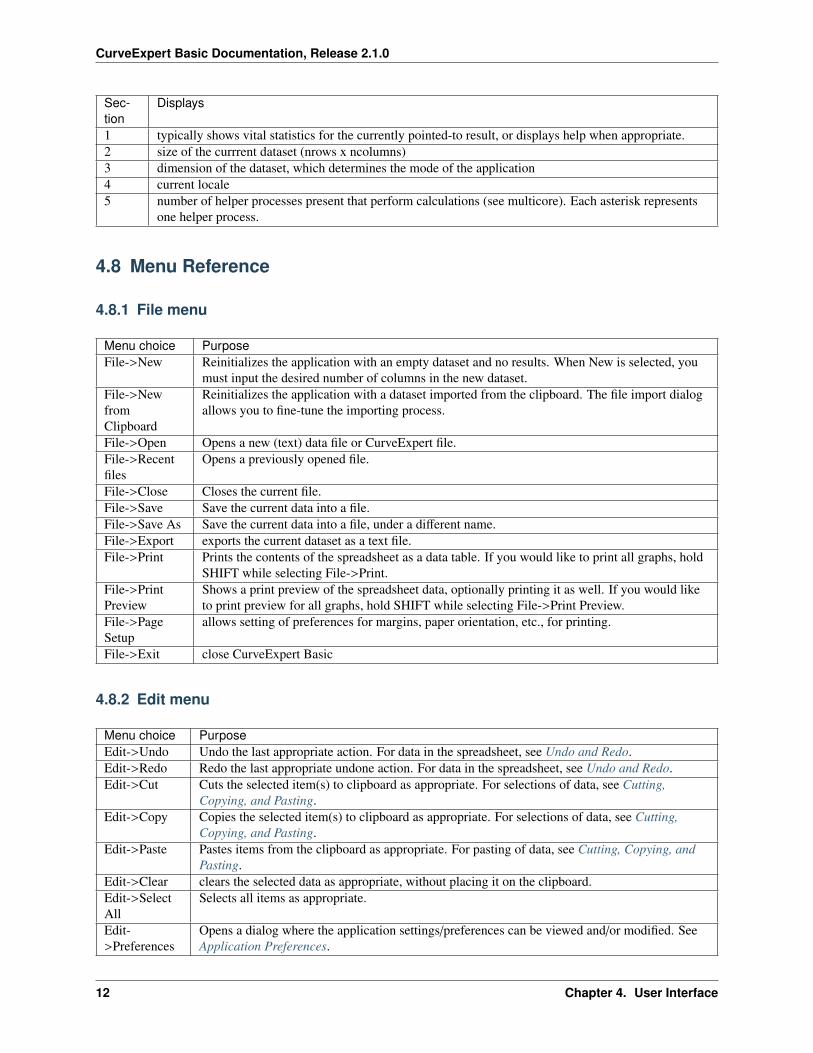
4.8 Menu Reference
4.8.1 File menu
Menu choice PurposeFile->New Reinitializes the application with an empty dataset and no results. When New is selected, you
must input the desired number of columns in the new dataset.File->NewfromClipboard
Reinitializes the application with a dataset imported from the clipboard. The file import dialogallows you to fine-tune the importing process.
File->Open Opens a new (text) data file or CurveExpert file.File->Recentfiles
Opens a previously opened file.
File->Close Closes the current file.File->Save Save the current data into a file.File->Save As Save the current data into a file, under a different name.File->Export exports the current dataset as a text file.File->Print Prints the contents of the spreadsheet as a data table. If you would like to print all graphs, hold
SHIFT while selecting File->Print.File->PrintPreview
Shows a print preview of the spreadsheet data, optionally printing it as well. If you would liketo print preview for all graphs, hold SHIFT while selecting File->Print Preview.
File->PageSetup
allows setting of preferences for margins, paper orientation, etc., for printing.
File->Exit close CurveExpert Basic
4.8.2 Edit menu
Menu choice PurposeEdit->Undo Undo the last appropriate action. For data in the spreadsheet, see Undo and Redo.Edit->Redo Redo the last appropriate undone action. For data in the spreadsheet, see Undo and Redo.Edit->Cut Cuts the selected item(s) to clipboard as appropriate. For selections of data, see Cutting,
Copying, and Pasting.Edit->Copy Copies the selected item(s) to clipboard as appropriate. For selections of data, see Cutting,
Copying, and Pasting.Edit->Paste Pastes items from the clipboard as appropriate. For pasting of data, see Cutting, Copying, and
Pasting.Edit->Clear clears the selected data as appropriate, without placing it on the clipboard.Edit->SelectAll
Selects all items as appropriate.
Edit->Preferences
Opens a dialog where the application settings/preferences can be viewed and/or modified. SeeApplication Preferences.
12 Chapter 4. User Interface
CurveExpert Basic Documentation, Release 2.1.0
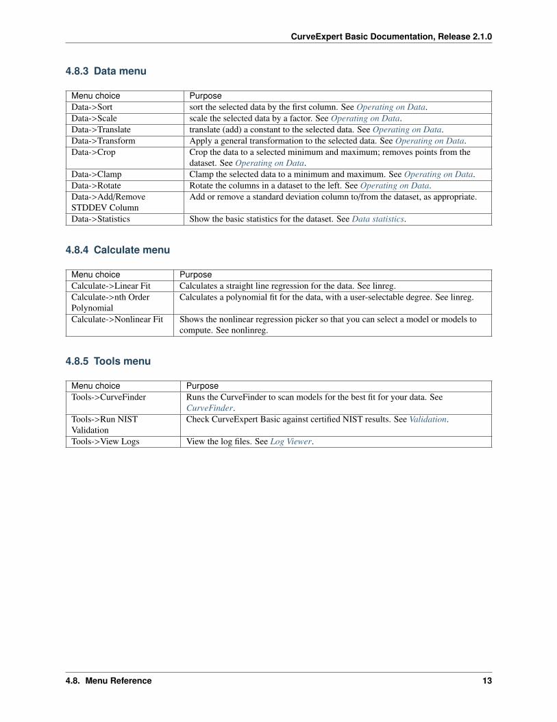
4.8.3 Data menu
Menu choice PurposeData->Sort sort the selected data by the first column. See Operating on Data.Data->Scale scale the selected data by a factor. See Operating on Data.Data->Translate translate (add) a constant to the selected data. See Operating on Data.Data->Transform Apply a general transformation to the selected data. See Operating on Data.Data->Crop Crop the data to a selected minimum and maximum; removes points from the
dataset. See Operating on Data.Data->Clamp Clamp the selected data to a minimum and maximum. See Operating on Data.Data->Rotate Rotate the columns in a dataset to the left. See Operating on Data.Data->Add/RemoveSTDDEV Column
Add or remove a standard deviation column to/from the dataset, as appropriate.
Data->Statistics Show the basic statistics for the dataset. See Data statistics.
4.8.4 Calculate menu
Menu choice PurposeCalculate->Linear Fit Calculates a straight line regression for the data. See linreg.Calculate->nth OrderPolynomial
Calculates a polynomial fit for the data, with a user-selectable degree. See linreg.
Calculate->Nonlinear Fit Shows the nonlinear regression picker so that you can select a model or models tocompute. See nonlinreg.
4.8.5 Tools menu
Menu choice PurposeTools->CurveFinder Runs the CurveFinder to scan models for the best fit for your data. See
CurveFinder.Tools->Run NISTValidation
Check CurveExpert Basic against certified NIST results. See Validation.
Tools->View Logs View the log files. See Log Viewer.
4.8. Menu Reference 13
CurveExpert Basic Documentation, Release 2.1.0
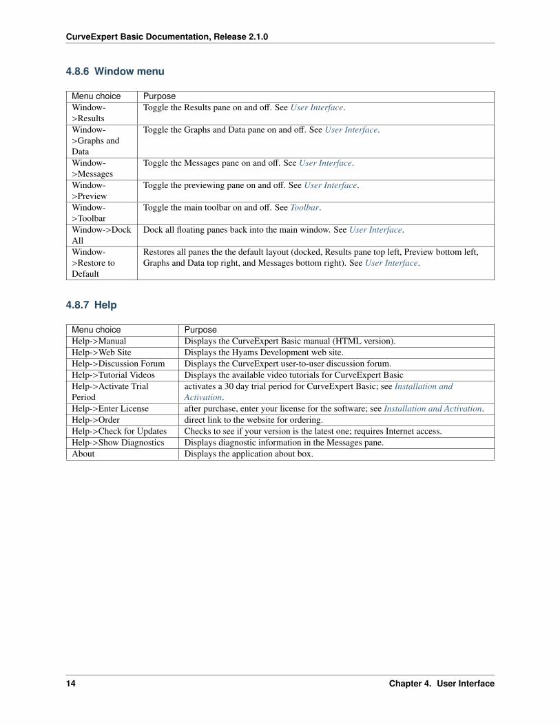
4.8.6 Window menu
Menu choice PurposeWindow->Results
Toggle the Results pane on and off. See User Interface.
Window->Graphs andData
Toggle the Graphs and Data pane on and off. See User Interface.
Window->Messages
Toggle the Messages pane on and off. See User Interface.
Window->Preview
Toggle the previewing pane on and off. See User Interface.
Window->Toolbar
Toggle the main toolbar on and off. See Toolbar.
Window->DockAll
Dock all floating panes back into the main window. See User Interface.
Window->Restore toDefault
Restores all panes the the default layout (docked, Results pane top left, Preview bottom left,Graphs and Data top right, and Messages bottom right). See User Interface.
4.8.7 Help
Menu choice PurposeHelp->Manual Displays the CurveExpert Basic manual (HTML version).Help->Web Site Displays the Hyams Development web site.Help->Discussion Forum Displays the CurveExpert user-to-user discussion forum.Help->Tutorial Videos Displays the available video tutorials for CurveExpert BasicHelp->Activate TrialPeriod
activates a 30 day trial period for CurveExpert Basic; see Installation andActivation.
Help->Enter License after purchase, enter your license for the software; see Installation and Activation.Help->Order direct link to the website for ordering.Help->Check for Updates Checks to see if your version is the latest one; requires Internet access.Help->Show Diagnostics Displays diagnostic information in the Messages pane.About Displays the application about box.
14 Chapter 4. User Interface
CHAPTER
FIVE
READING DATA
5.1 Introduction
The first task in any data analysis program like CurveExpert Basic is to read or import your data into the software.For this, CurveExpert Basic provides a robust file import mechanism, which can be accessed simply by choosingFile->Open. You can read in both native CurveExpert files (.cxp) and generic data files in text format.
Note: To be able to choose files with extensions other than .cxp, you must select the appropriate extension in thebottom right corner of the file choosing dialog.
Most of the time, the data to be read in is contained within a text file of some sort, with headers and commentsinterspersed. CurveExpert Basic tries to make the job of importing this data as easy and painless as possible. The fileimport intelligently examines your raw file in order to find the data, as well as finding column headers for that data, ifpresent.
5.2 Raw file import
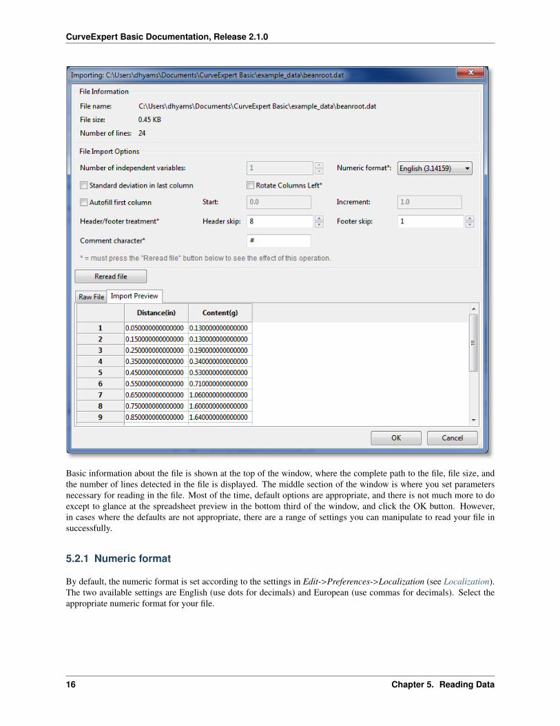
To read in a text file (common extensions are .dat and .txt, but can be anything that you choose), simply choose File->Open, and then the filename. Alternatively, drag and drop the file to the CurveExpert Basic spreadsheet. The fileimport window will display, as follows:
15
CurveExpert Basic Documentation, Release 2.1.0
Basic information about the file is shown at the top of the window, where the complete path to the file, file size, andthe number of lines detected in the file is displayed. The middle section of the window is where you set parametersnecessary for reading in the file. Most of the time, default options are appropriate, and there is not much more to doexcept to glance at the spreadsheet preview in the bottom third of the window, and click the OK button. However,in cases where the defaults are not appropriate, there are a range of settings you can manipulate to read your file insuccessfully.
5.2.1 Numeric format
By default, the numeric format is set according to the settings in Edit->Preferences->Localization (see Localization).The two available settings are English (use dots for decimals) and European (use commas for decimals). Select theappropriate numeric format for your file.
16 Chapter 5. Reading Data
CurveExpert Basic Documentation, Release 2.1.0
5.2.2 Rotate columns left
Some raw datasets list the dependent variable first. If this is the case, checking Rotate columns left will shift thedata in the first column to the last, moving all other columns to the left. This is the ordering that CurveExpert Basicexpects (independent variables first, and the dependent variable following). For a two column dataset, this operationis equivalent to swapping the columns. To see the effects of your choice here, the Reread file button must be pressed.
5.2.3 Autofill
Sometimes, the independent variable is implied by the ordering of the data. If you would like to generate the firstcolumn of data as a simple range and increment, select Autofill first column, and then choose the starting value andincrement between each data point. The result of your operation is shown instantly in the spreadsheet preview. Thefill is computed as follows:
x = xstart + i∆x
where i is the point id (starting at zero for the first point), xstart is the starting value input, and ∆x is the incrementinput.
5.2.4 Treatment of Header and Footer
Often, data files have text that is not part of the dataset, and this text appears either before or after the real dataset (orboth). To accommodate for this, you can set the Header Skip and Footer Skip, which is the number of lines in the filethat are skipped at the top and bottom, respectively, before any attempt is made at reading data. This capability canalso be used to intentionally skip over certain data in your file.
The header and footer skip can be thought of as a mask that is applied to your file before any reading takes place.
CurveExpert Basic uses a sophisticated procedure to try to guess the header and footer skip correctly. In all but themost esoteric cases, the header and footer skips will be correct already, and therefore need no interaction from the user.
Note: A newline at the end of your file counts as just that; a new line. This line is skipped by CurveExpert Basicbecause it is a line with no data. Therefore, it is common for the footer skip to be set to 1 by the automatic header/footeralgorithm.
5.2.5 Comment character
Most data files have comments interspersed throughout them, sometimes in the middle of the data. In order to skipthese comments, the character that designates the comment must be specified. In the data file, then, anything thatappears after a comment character is ignored. Common comment characters are ‘#’ and ‘%’.
5.2.6 Refreshing the preview
If rotating columns or changing the header/footer treatment, you must press the Reread file button to refresh thepreview.
5.2. Raw file import 17
CurveExpert Basic Documentation, Release 2.1.0
5.2.7 File import preview and raw file preview
The file import preview shows the result of the reading of the file, augmented by the current settings discussed above.This preview shows you exactly what CurveExpert Basic will read and place in the main spreadsheet.
The raw file preview shows you a copy of the file, with no modification, so that you can see the contents. Line numbersare annotated on the left, the the header and footer skip settings are shown by dimming the areas of the file that aremasked away by these settings.
5.2.8 Column Labels
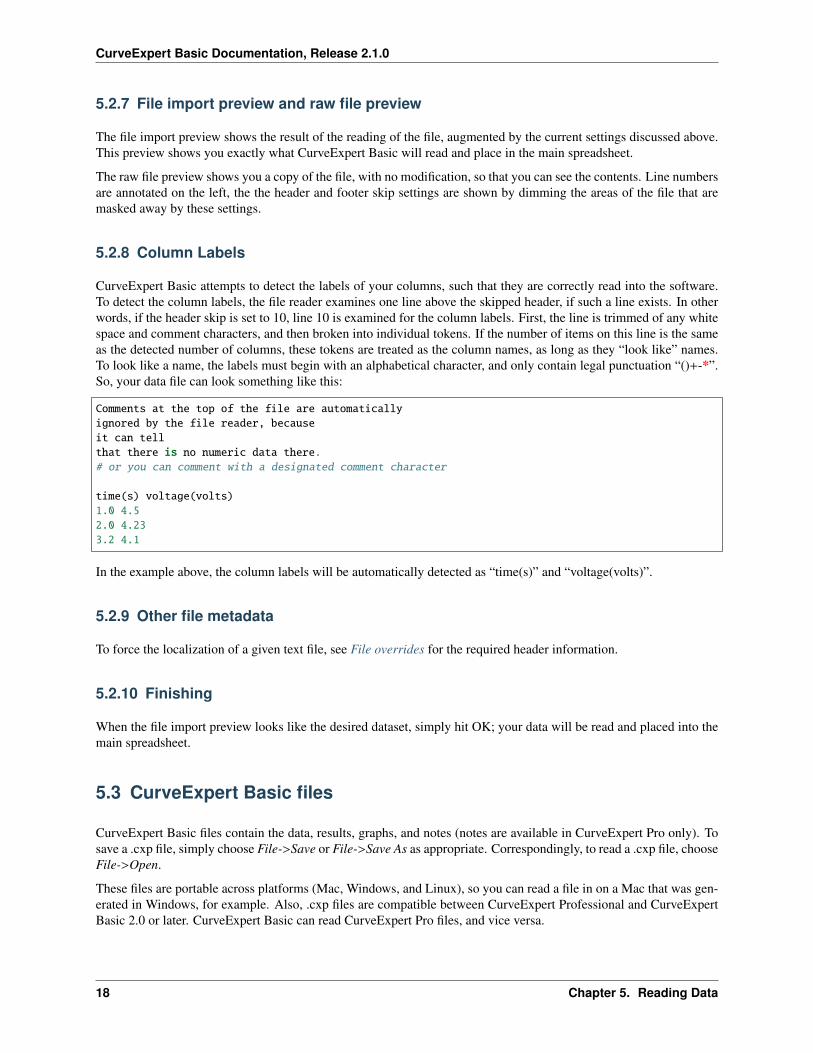
CurveExpert Basic attempts to detect the labels of your columns, such that they are correctly read into the software.To detect the column labels, the file reader examines one line above the skipped header, if such a line exists. In otherwords, if the header skip is set to 10, line 10 is examined for the column labels. First, the line is trimmed of any whitespace and comment characters, and then broken into individual tokens. If the number of items on this line is the sameas the detected number of columns, these tokens are treated as the column names, as long as they “look like” names.To look like a name, the labels must begin with an alphabetical character, and only contain legal punctuation “()+-*”.So, your data file can look something like this:
Comments at the top of the file are automaticallyignored by the file reader, becauseit can tellthat there is no numeric data there.# or you can comment with a designated comment character
time(s) voltage(volts)1.0 4.52.0 4.233.2 4.1
In the example above, the column labels will be automatically detected as “time(s)” and “voltage(volts)”.
5.2.9 Other file metadata
To force the localization of a given text file, see File overrides for the required header information.
5.2.10 Finishing
When the file import preview looks like the desired dataset, simply hit OK; your data will be read and placed into themain spreadsheet.
5.3 CurveExpert Basic files
CurveExpert Basic files contain the data, results, graphs, and notes (notes are available in CurveExpert Pro only). Tosave a .cxp file, simply choose File->Save or File->Save As as appropriate. Correspondingly, to read a .cxp file, chooseFile->Open.
These files are portable across platforms (Mac, Windows, and Linux), so you can read a file in on a Mac that was gen-erated in Windows, for example. Also, .cxp files are compatible between CurveExpert Professional and CurveExpertBasic 2.0 or later. CurveExpert Basic can read CurveExpert Pro files, and vice versa.
18 Chapter 5. Reading Data

CurveExpert Basic Documentation, Release 2.1.0
Also, if a particular model or function is saved as a result in a .cxp file and it is not present on the system reading thefile, the model/function will automatically be created on your behalf. This newly created model/function will then beavailable for use in the “Imported” family, and will appear appropriately in the Nonlinear model or function pickers.
5.3. CurveExpert Basic files 19

CurveExpert Basic Documentation, Release 2.1.0
20 Chapter 5. Reading Data
CHAPTER
SIX
WORKING WITH DATA
6.1 Introduction
The raw data in CurveExpert Basic is handled as a simple matrix of numbers; the dataset is made up of a number ofrows and a number of columns. The first column is interpreted as the independent variable, and the second column isinterpreted as the dependent variable.
6.2 Data statistics
Simple statistics for the current dataset can be obtained by selecting Data->Statistics. The resulting window willdisplay the number of points and columns, and the following stats for each column of your dataset:
• minimum
• maximum
• range
• average (mean)
• standard deviation
The average is computed with the standard formula:
x =1N
N∑i=1
xi
Standard deviation is computed with the following formula, which is called the standard deviation of the sample:
σ =
⎯1N
N∑i=1
(xi − x)2
To copy the statistics information to the clipboard, press the Copy button at the bottom of the dialog.
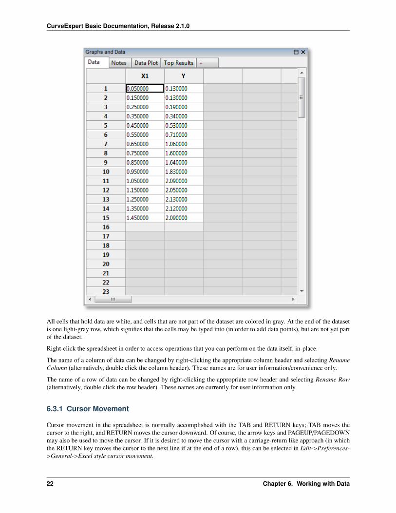
6.3 The spreadsheet
The spreadsheet resides in the “Graphs and Data” pane in CurveExpert Basic.
The spreadsheet allows manual entry or modification of a dataset either entry-by-entry, or by cutting and pasting fromwithin CurveExpert Basic, or from other sources. An example of the spreadsheet is shown below;
21
CurveExpert Basic Documentation, Release 2.1.0
All cells that hold data are white, and cells that are not part of the dataset are colored in gray. At the end of the datasetis one light-gray row, which signifies that the cells may be typed into (in order to add data points), but are not yet partof the dataset.
Right-click the spreadsheet in order to access operations that you can perform on the data itself, in-place.
The name of a column of data can be changed by right-clicking the appropriate column header and selecting RenameColumn (alternatively, double click the column header). These names are for user information/convenience only.
The name of a row of data can be changed by right-clicking the appropriate row header and selecting Rename Row(alternatively, double click the row header). These names are currently for user information only.
6.3.1 Cursor Movement
Cursor movement in the spreadsheet is normally accomplished with the TAB and RETURN keys; TAB moves thecursor to the right, and RETURN moves the cursor downward. Of course, the arrow keys and PAGEUP/PAGEDOWNmay also be used to move the cursor. If it is desired to move the cursor with a carriage-return like approach (in whichthe RETURN key moves the cursor to the next line if at the end of a row), this can be selected in Edit->Preferences->General->Excel style cursor movement.
22 Chapter 6. Working with Data
CurveExpert Basic Documentation, Release 2.1.0
To reverse the direction of cursor navigation, hold the SHIFT key.
6.3.2 Cutting, Copying, and Pasting
When copying data, the current selection in the spreadsheet is placed on the clipboard (and obeys your regional settingswhile doing so). If no data is selected, all data is copied. The delimiter used between columns, if applicable, is thedelimiter chosen in Edit->Preferences->General->Default Delimiter.
A “cut” must involve all columns of the dataset. Therefore, the “Cut” item in the data menu is dimmed if your selectiononly involves some of the columns. This behavior is due to the fact that a cut will remove points from the dataset, andyour selection should reflect that reality.
A paste from the clipboard informs CurveExpert Basic to attempt to intelligently read what is on the clipboard andturn that into an intermediate dataset for subsequent pasting. Different rows in this intermediate dataset are delimitedby newlines (or carriage returns), and columns are delimited by whitespace or commas (unless using European formatfor incoming numbers, in which case commas are not valid as a delimiter). This intermediate dataset will then beinserted at the current cursor location in the spreadsheet, overwriting parts of your existing dataset and extending yourexisting dataset as necessary. A paste operation can be viewed as an insertion of a block of data at the current cursorlocation, following by a subsequent discarding of any data that happens to fall outside the current number of columnsof your dataset.
6.3.3 Inserting Rows
To insert a row into your dataset, right click on the spreadsheet and select “Insert Row”. This will cause all rows ator below the current cursor location (indicated by the black outline) to be shifted downwards, and a new row will beinserted at the current location.
To insert multiple rows at once, select a range in the spreadsheet, right click, and select “Insert Row” as before. Inthis case, all rows touched by the selection will be shifted downwards, and new rows are inserted at the current cursorlocation. The number of inserted rows will equal the number of rows in the original selection. For example, to insertthree rows at row 2, select rows 2-4 (inclusive) and select “Insert Row”.
6.3.4 Removing Rows
To remove rows from the dataset, select a set of rows to be removed, right click, and select “Remove Rows”. This isfunctionally similar to cutting the rows (see above), except that the data is not copied to the clipboard.
6.3.5 Undo and Redo
All data operations are undoable and redoable to a number of levels possible by the Edit->Preferences->Advanced->Peak Undo Memory Usage setting. All data operations are undoable and redoable to a number of levels possible bythe Edit->Preferences->Advanced->Number of undo levels setting. So, you can feel comfortable manipulating dataknowing that any transformation, clear, or cut/paste operation can be undone.
6.4 Number Formatting
The values shown in a spreadsheet may be formatted by selecting a block via the mouse, right clicking, and selectingFormat Numbers from the resulting menu. A dialog will appear as follows:
A General formatting prints a number naturally as most practitioners would write the number. Scientific formattingprints the number always with a mantissa and exponent part, as in “1.532e+04”. Engineering formatting is almost
6.4. Number Formatting 23
CurveExpert Basic Documentation, Release 2.1.0
the same as scientific, but the exponent is always guaranteed to be a multiple of three. Percentage formatting shows adecimal as a percentage, with a following percentage sign. For example, the number 0.05 would be shown as 5.0%.
The Decimal places field allows the user to specify the number of decimal places shown; this setting is relevant for allformatting settings listed above except for General.
The Leader and Trailer fields allow the user to place customized text before and/or after the number. These fieldsare very useful for adding units to numbers (use the trailer) or prepending a dollar sign for currencies (place $ in theLeader field).
6.5 Operating on Data
CurveExpert Basic provides several ways that you can operate on raw data in the spreadsheet. To perform theseoperations, simply highlight the data that you want to work on, and select one of Sort, Scale, Translate, Transform,Crop, or Clamp from the Data menu. Alternatively, you can right click on the spreadsheet after making a selection. Ifno selection is made, the operation is assumed to apply to the entire dataset (all rows and all columns).
6.5.1 Sort
To sort your data against the first column of the dataset, select Sort from the Data menu (the entire dataset must beselected in the spreadsheet). If CurveExpert Basic has detected that the data is already sorted, this menu item will bedimmed. If the choice is nondimmed, however, it does not necessarily mean that the dataset is already sorted.
6.5.2 Scale
To multiply by or divide the selected data by a factor, select Data->Scale.
6.5.3 Translate
To add a constant value to the selected data, select Data->Translate.
6.5.4 Crop
To drop points from the selected part of your dataset that are above or below a certain threshhold, select Data->Crop.After a cropping operation, there is likely to be fewer data points in your data set than before the crop. Usually,cropping is used to eliminate outliers from a dataset.
6.5.5 Clamp
To clamp points in the selected part of your dataset to a certain threshhold value, select Data->Clamp. Clamping isusually used to correct values that are slightly over or under a valid domain for that value.
6.5.6 Rotate
To rotate columns in a dataset, select Data->Rotate. For a dataset with two columns, this is exactly the same as acolumn swap. Note that the rotation always proceeds to the left in a circular fashion; the leftmost column becomes therightmost one after the rotation, and all other columns are displaced by one to the left.
24 Chapter 6. Working with Data
CurveExpert Basic Documentation, Release 2.1.0
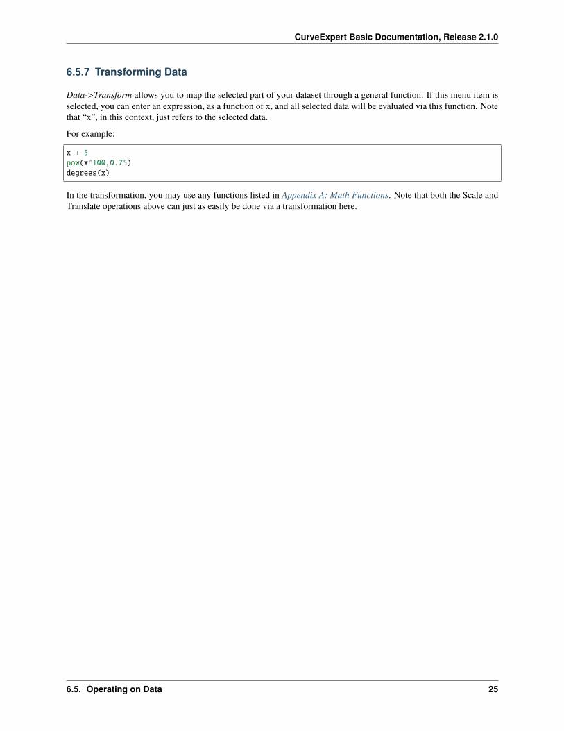
6.5.7 Transforming Data
Data->Transform allows you to map the selected part of your dataset through a general function. If this menu item isselected, you can enter an expression, as a function of x, and all selected data will be evaluated via this function. Notethat “x”, in this context, just refers to the selected data.
For example:
x + 5pow(x*100,0.75)degrees(x)
In the transformation, you may use any functions listed in Appendix A: Math Functions. Note that both the Scale andTranslate operations above can just as easily be done via a transformation here.
6.5. Operating on Data 25

CurveExpert Basic Documentation, Release 2.1.0
26 Chapter 6. Working with Data
CHAPTER
SEVEN
CALCULATING RESULTS
CurveExpert Basic supports TWO distinct classes of results:
• regressions
– linear regressions (linear and polynomial fits)
– nonlinear regressions (built-in and custom models)
• interpolations
– cubic spline
– tension spline
Calculation of these results can be accessed through the Calculate menu in CurveExpert Basic, or optionally via thecorresponding buttons on the toolbar (see Toolbar).
7.1 General Guidelines
7.1.1 Scaling Datasets
For best results, always scale your data sets to the order of one. You may do this prior to reading in your data file, orafter your data file has been imported using the scaling feature in CurveExpert Basic (see Operating on Data).
Imagine a data set with x values ranging from 1000 to 10000 and a regression model where the term exp(a*x) isinvolved. Unless a very good initial guess for a is given, chances are that an exponential to a very large power(eg. exp(1000)) will be taken in the course of the nonlinear regression algorithm. The calculation will overflow,and the regression will fail as a result. Even if the regression happens not to fail, the regression algorithm will havean exceedingly tough time finding the correct parameters, since a small change in the free parameters will cause atremendous change in the size of the term. The moral of the story: always scale your data!
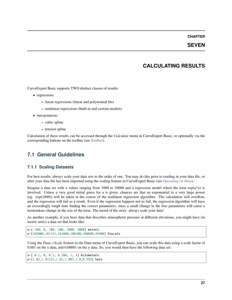
As another example, if you have data that describes atmospheric pressure at different elevations, you might have (inmetric units) a data set that looks like:
x=[-100, 0, 100, 500, 1000, 4000] metersy=[102000,101325,101000,100500,100000,99900] Pascals
Using the Data->Scale feature in the Data menu of CurveExpert Basic, you can scale this data using a scale factor of0.001 on the x data, and 0.00001 on the y data. So, you would then have the following data set:
x=[-0.1, 0, 0.1, 0.500, 1, 4] kilometersy=[1.02,1.01325,1.01,1.005,1.0,0.999] bars
27
CurveExpert Basic Documentation, Release 2.1.0
The second example is much more likely to allow nonlinear regressions to converge, and also will allow higher orderpolynomial fits to be performed with more accuracy. If you have a data set that seems particularly ill-behaved, scalingcan help solve this problem.
Note that CurveExpert Basic is able to perform correctly on data in any scale, as long as the calculations do notoverflow or underflow. So, if a data set is giving problems, scaling it should be the first action to take.
7.1.2 Set the tolerance parameter reasonably
Don’t set the tolerance parameter (in Edit->Preferences->Regression) too low. In regression modeling, not muchadvantage is to be gained by setting a very strict tolerance. Its main purpose in life is to prevent the nonlinear regressionalgorithm from converging on local minima, not to make the calculated parameters more accurate.
7.1.3 Data should be appropriate to the model
Make sure that the data is appropriate to the model. Especially look out for using logarithmic or exponential familiesof models with data that contains zeros or negatives. For example, it is not possible, in any shape or form, to obtain anegative or zero with the basic exponential model (y=ae^(bx), assuming a is positive; the inverse problem exists for anegative a). So, it is not wise to use a model that cannot reflect the trends in the data.
7.1.4 Sometimes, it is unavoidable
Some curve fits are simply ill-behaved, i.e. prone to divergence. For some data sets, it may not be possible to convergecertain nonlinear regression models.
7.2 Interpolation
7.2.1 Introduction
An interpolation, by definition, passes through every data point, and as such, the correlation coefficient will alwaysbe 1, and the standard error will always be zero. CurveExpert Basic supports cubic splines and tension splines. Allsplines are defined in a piecewise fashion between data points.
Note: The dataset must be sorted (based on the independent variable) in order for any spline interpolation to work.Select Data->Sort from the main menu in order to sort your dataset if necessary. If CurveExpert Basic detects thatyour dataset is not sorted, it will not allow spline interpolations to be selected.
7.2.2 Cubic Splines
To calculate a cubic spline, select Calculate->Cubic Spline from the main menu. The cubic spline is simply a polyno-mial spline of order 3; cubic splines are the most common form of spline. Cubic splines guarantee continuity in thespline, and continuity in the first and second derivatives of the spline at the data points. At the endpoints, the secondderivative is set to zero, which is termed a “natural” spline at the endpoints, as the curvature goes to zero.
28 Chapter 7. Calculating Results
CurveExpert Basic Documentation, Release 2.1.0
7.2.3 Tension Splines
To calculate a tension spline, select Calculate->Tension Spline from the main menu. A prompt will appear to ask forthe amount of tension desired. Tension splines are based on hyperbolic functions, and simulate a cord being stretchedwith a defined tension (amount of force) between the data points. An extremely high tension approaches a linearspline, and low tensions will appear correspondingly “loose” around the data points, resembling a cubic spline.
7.3 Linear Regression
7.3.1 Introduction
Linear regressions, as a class of results, can be calculated directly, and do not need an iterative process like nonlinearregressions do. See Linear Regression in the appendices for a more in-depth explanation. A linear regression can beconstructed from any model that is a linear combination of functions; the coefficients in the linear combination are theparameters to be found.
There are two types of linear regressions supported in CurveExpert: linear and polynomial. All other regressions,even if they could be calculated as a linear-type regression through a variable transformation, are computed with thenonlinear regression engine.
7.3.2 Linear Fit
In CurveExpert Basic, you can choose to calculate a straight line regression:
y = ax + b
by choosing Calculate->Linear Fit.
7.3.3 nth Order Polynomial Fit
To calculate a polynomial via linear regression, choose Calculate->nth Order Polynomial Fit. A prompt will appear toask for the degree of polynomial desired. Also, in the same prompt, you can choose to force the polynomial throughthe origin, which forces the intercept to zero. Also, you may choose the desired weighting for each point in the dataset(see weighting for further information) After entering the degree (and origin forcing or weighting as appropriate), thepolynomial will be computed and added to the result list.
7.4 Nonlinear Regression
7.4.1 Introduction
Nonlinear regressions are solved with the Marquart-Levenberg method as documented in Nonlinear Regression in theappendices. To calculate a nonlinear regression, select Calculate->Nonlinear Model Fit from the main menu.
7.4.2 Selecting a Model or Models
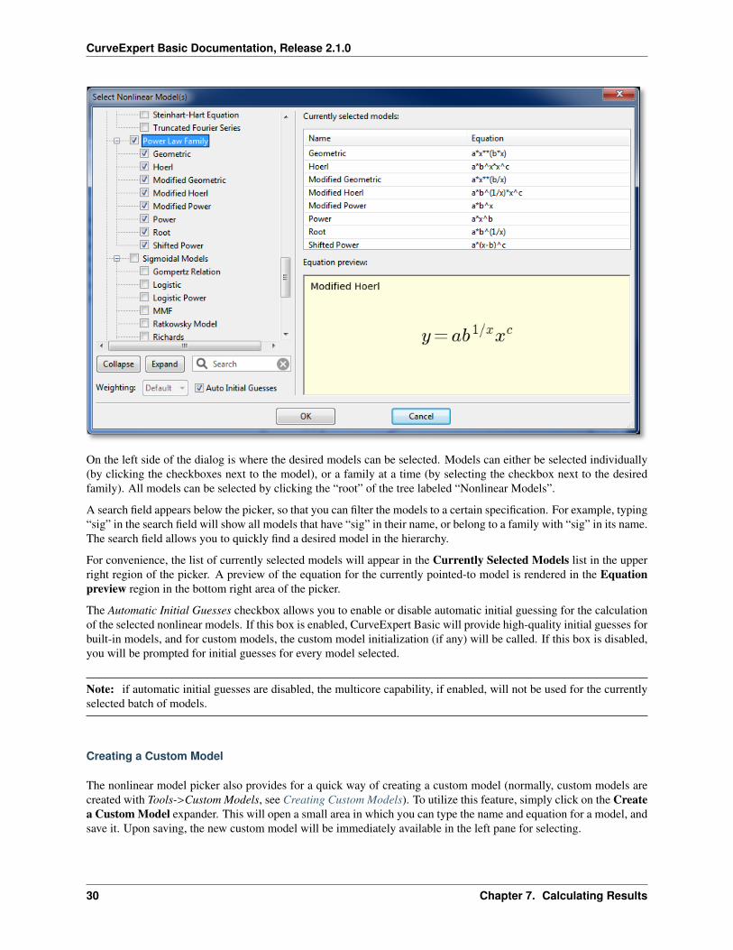
Upon selecting Calculate->Nonlinear Model Fit, the nonlinear regression picker will appear; all models appear in thispicker (built-in models and custom models) that are appropriate for the number of independent variables in the dataset.A screenshot of the model picker is below:
7.3. Linear Regression 29
CurveExpert Basic Documentation, Release 2.1.0
On the left side of the dialog is where the desired models can be selected. Models can either be selected individually(by clicking the checkboxes next to the model), or a family at a time (by selecting the checkbox next to the desiredfamily). All models can be selected by clicking the “root” of the tree labeled “Nonlinear Models”.
A search field appears below the picker, so that you can filter the models to a certain specification. For example, typing“sig” in the search field will show all models that have “sig” in their name, or belong to a family with “sig” in its name.The search field allows you to quickly find a desired model in the hierarchy.
For convenience, the list of currently selected models will appear in the Currently Selected Models list in the upperright region of the picker. A preview of the equation for the currently pointed-to model is rendered in the Equationpreview region in the bottom right area of the picker.
The Automatic Initial Guesses checkbox allows you to enable or disable automatic initial guessing for the calculationof the selected nonlinear models. If this box is enabled, CurveExpert Basic will provide high-quality initial guesses forbuilt-in models, and for custom models, the custom model initialization (if any) will be called. If this box is disabled,you will be prompted for initial guesses for every model selected.
Note: if automatic initial guesses are disabled, the multicore capability, if enabled, will not be used for the currentlyselected batch of models.
Creating a Custom Model
The nonlinear model picker also provides for a quick way of creating a custom model (normally, custom models arecreated with Tools->Custom Models, see Creating Custom Models). To utilize this feature, simply click on the Createa Custom Model expander. This will open a small area in which you can type the name and equation for a model, andsave it. Upon saving, the new custom model will be immediately available in the left pane for selecting.
30 Chapter 7. Calculating Results
CurveExpert Basic Documentation, Release 2.1.0
7.4.3 Setting the Weighting Scheme
To set the weighting scheme desired for the models that are to be computed, select the weighting scheme from thechooser at the bottom left of the dialog. See weighting for further details on the weighting schemes.
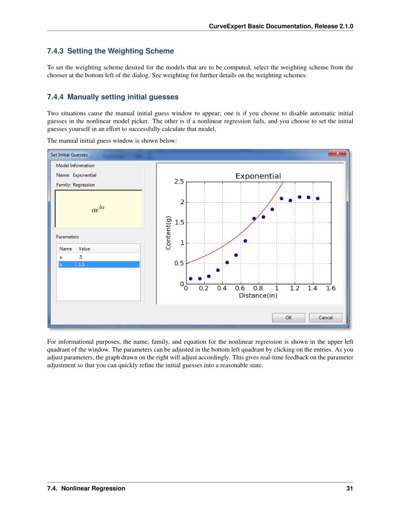
7.4.4 Manually setting initial guesses
Two situations cause the manual initial guess window to appear; one is if you choose to disable automatic initialguesses in the nonlinear model picker. The other is if a nonlinear regression fails, and you choose to set the initialguesses yourself in an effort to successfully calculate that model.
The manual initial guess window is shown below:
For informational purposes, the name, family, and equation for the nonlinear regression is shown in the upper leftquadrant of the window. The parameters can be adjusted in the bottom left quadrant by clicking on the entries. As youadjust parameters, the graph drawn on the right will adjust accordingly. This gives real-time feedback on the parameteradjustment so that you can quickly refine the initial guesses into a reasonable state.
7.4. Nonlinear Regression 31

CurveExpert Basic Documentation, Release 2.1.0
32 Chapter 7. Calculating Results
CHAPTER
EIGHT
CURVEFINDER
8.1 Usage
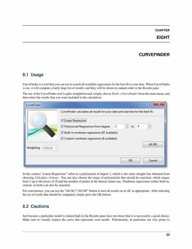
CurveFinder is a tool that you can use to search all available regressions for the best fit to your data. When CurveFinderis run, it will compute a fairly large list of results, and they will be shown in ranked order in the Results pane.
The use of the CurveFinder tool is quite straightforward; simply choose Tools->CurveFinder from the main menu, andthen select the results that you want included in the calculation.
In this context “Linear Regression” refers to a polynomial of degree 1, which is the same straight line obtained fromchoosing Calculate->Linear. You can also choose the range of polynomials that should be searched, which rangesfrom 2 up to the lesser of 20 and the number of points in the dataset minus one. Nonlinear regressions (either built-in,custom, or both) can also be searched.
For convenience, you can use the “All On”/”All Off” button to turn all results on or off, as appropriate. After selectingthe set of results that should be computed, simply press the OK button.
8.2 Cautions
Just because a particular model is ranked high in the Results pane does not mean that it is necessarily a good choice.Make sure to visually inspect the curve that represents your model. Polynomials, in particular, are very prone to
33

CurveExpert Basic Documentation, Release 2.1.0
oscillation, and can veer wildly away from the dataset before returning to be near the data points at each x value. Makesure that the model that you choose as best is a reasonable representation of your data.
34 Chapter 8. CurveFinder
CHAPTER
NINE
WORKING WITH RESULTS
9.1 Introduction
Once any results have been calculated, they appear in the result pane ranked in order of their score (the result panenormally is shown in the upper left part of the CurveExpert Basic application, see User Interface). The score reflectshow closely the model adheres to the underlying data.
In the results pane, the results can also be sorted by any of the items displayed in the column header (name, kind, family,score, correlation coefficient, coefficient of determination, or standard error) simply by clicking the appropriate columnheader. Note that you can right-click on the column header in order to customize what is displayed in the results list;by default, the name, kind, and score is displayed.
When selecting results, you can simply click on the result (which selects it), or use multiple selection by holding downSHIFT or CTRL when clicking on results. This allows you to apply an operation to batches of results at once.
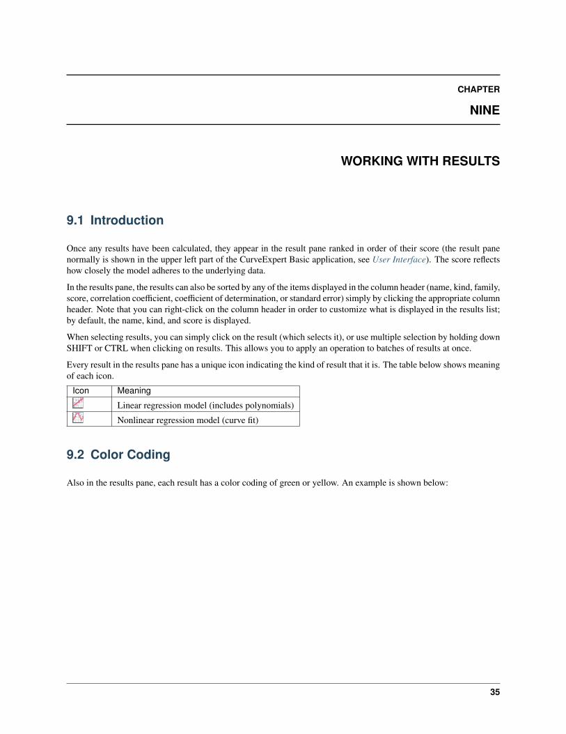
Every result in the results pane has a unique icon indicating the kind of result that it is. The table below shows meaningof each icon.
Icon Meaning
Linear regression model (includes polynomials)
Nonlinear regression model (curve fit)
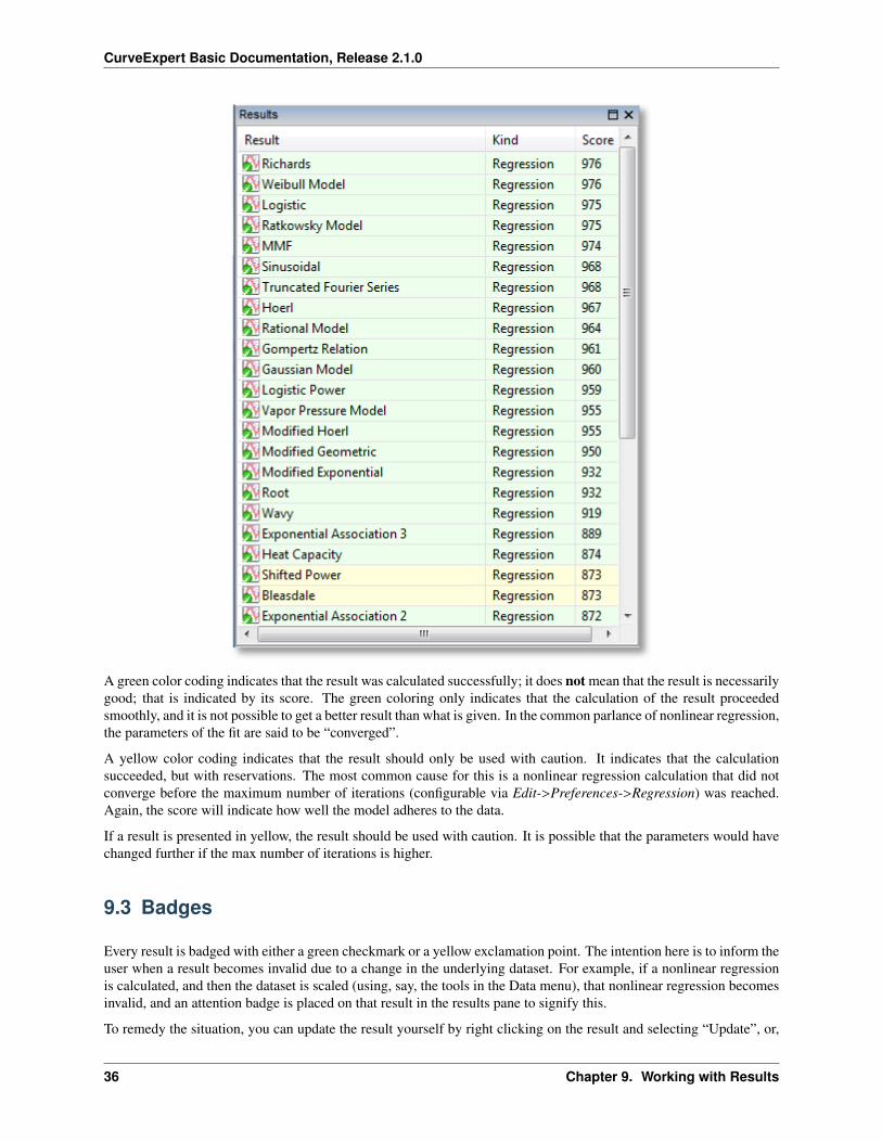
9.2 Color Coding
Also in the results pane, each result has a color coding of green or yellow. An example is shown below:
35
CurveExpert Basic Documentation, Release 2.1.0
A green color coding indicates that the result was calculated successfully; it does not mean that the result is necessarilygood; that is indicated by its score. The green coloring only indicates that the calculation of the result proceededsmoothly, and it is not possible to get a better result than what is given. In the common parlance of nonlinear regression,the parameters of the fit are said to be “converged”.
A yellow color coding indicates that the result should only be used with caution. It indicates that the calculationsucceeded, but with reservations. The most common cause for this is a nonlinear regression calculation that did notconverge before the maximum number of iterations (configurable via Edit->Preferences->Regression) was reached.Again, the score will indicate how well the model adheres to the data.
If a result is presented in yellow, the result should be used with caution. It is possible that the parameters would havechanged further if the max number of iterations is higher.
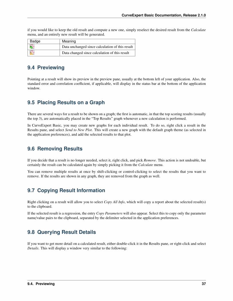
9.3 Badges
Every result is badged with either a green checkmark or a yellow exclamation point. The intention here is to inform theuser when a result becomes invalid due to a change in the underlying dataset. For example, if a nonlinear regressionis calculated, and then the dataset is scaled (using, say, the tools in the Data menu), that nonlinear regression becomesinvalid, and an attention badge is placed on that result in the results pane to signify this.
To remedy the situation, you can update the result yourself by right clicking on the result and selecting “Update”, or,
36 Chapter 9. Working with Results
CurveExpert Basic Documentation, Release 2.1.0
if you would like to keep the old result and compute a new one, simply reselect the desired result from the Calculatemenu, and an entirely new result will be generated.
Badge MeaningData unchanged since calculation of this result
Data changed since calculation of this result
9.4 Previewing
Pointing at a result will show its preview in the preview pane, usually at the bottom left of your application. Also, thestandard error and correlation coefficient, if applicable, will display in the status bar at the bottom of the applicationwindow.
9.5 Placing Results on a Graph
There are several ways for a result to be shown on a graph; the first is automatic, in that the top scoring results (usuallythe top 3), are automatically placed in the “Top Results” graph whenever a new calculation is performed.
In CurveExpert Basic, you may create new graphs for each individual result. To do so, right click a result in theResults pane, and select Send to New Plot. This will create a new graph with the default graph theme (as selected inthe application preferences), and add the selected results to that plot.
9.6 Removing Results
If you decide that a result is no longer needed, select it, right click, and pick Remove. This action is not undoable, butcertainly the result can be calculated again by simply picking it from the Calculate menu.
You can remove multiple results at once by shift-clicking or control-clicking to select the results that you want toremove. If the results are shown in any graph, they are removed from the graph as well.
9.7 Copying Result Information
Right clicking on a result will allow you to select Copy All Info, which will copy a report about the selected result(s)to the clipboard.
If the selected result is a regression, the entry Copy Parameters will also appear. Select this to copy only the parametername/value pairs to the clipboard, separated by the delimiter selected in the application preferences.
9.8 Querying Result Details
If you want to get more detail on a calculated result, either double-click it in the Results pane, or right-click and selectDetails. This will display a window very similar to the following:
9.4. Previewing 37
CurveExpert Basic Documentation, Release 2.1.0
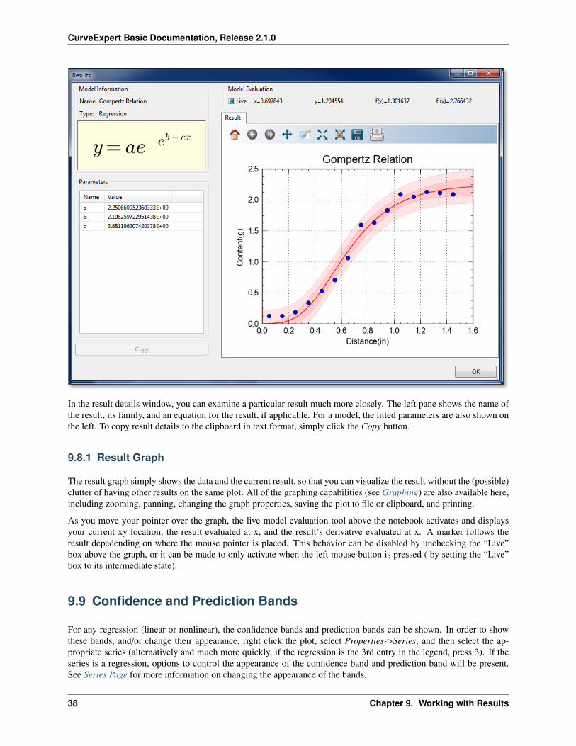
In the result details window, you can examine a particular result much more closely. The left pane shows the name ofthe result, its family, and an equation for the result, if applicable. For a model, the fitted parameters are also shown onthe left. To copy result details to the clipboard in text format, simply click the Copy button.
9.8.1 Result Graph
The result graph simply shows the data and the current result, so that you can visualize the result without the (possible)clutter of having other results on the same plot. All of the graphing capabilities (see Graphing) are also available here,including zooming, panning, changing the graph properties, saving the plot to file or clipboard, and printing.
As you move your pointer over the graph, the live model evaluation tool above the notebook activates and displaysyour current xy location, the result evaluated at x, and the result’s derivative evaluated at x. A marker follows theresult depedending on where the mouse pointer is placed. This behavior can be disabled by unchecking the “Live”box above the graph, or it can be made to only activate when the left mouse button is pressed ( by setting the “Live”box to its intermediate state).
9.9 Confidence and Prediction Bands
For any regression (linear or nonlinear), the confidence bands and prediction bands can be shown. In order to showthese bands, and/or change their appearance, right click the plot, select Properties->Series, and then select the ap-propriate series (alternatively and much more quickly, if the regression is the 3rd entry in the legend, press 3). If theseries is a regression, options to control the appearance of the confidence band and prediction band will be present.See Series Page for more information on changing the appearance of the bands.
38 Chapter 9. Working with Results

CurveExpert Basic Documentation, Release 2.1.0
The confidence band is the area that has a certain likelihood (typically 95%, but you can adjust the level to your liking)of containing the true curve that fits the data.
The prediction band is the area that has a certain likelihood (typically 95%, but you can adjust the level to your liking)of containing any future data points. The prediction band is always wider than the confidence band.
9.9. Confidence and Prediction Bands 39

CurveExpert Basic Documentation, Release 2.1.0
40 Chapter 9. Working with Results
CHAPTER
TEN
GRAPHING
10.1 Introduction
CurveExpert Basic contains a fully-featured graphing engine. The graphs are publication quality and are fully an-tialiased for the best possible appearance. The easiest way to generate a plot from a result (in the “Results” pane) is toright click the result, and select “Send to New Plot”.
10.2 Graph Types
There are is one type of graph supported by CurveExpert Basic; standard XY plots. More graph types are supportedin CurveExpert Pro.
10.2.1 XY Plots
XY plots, by definition, have two axes in Cartesian space. XY plots are appropriate for showing relationships betweencause and effect, or equivalently, the relationship between one independent variable and one dependent variable.
10.3 Basics
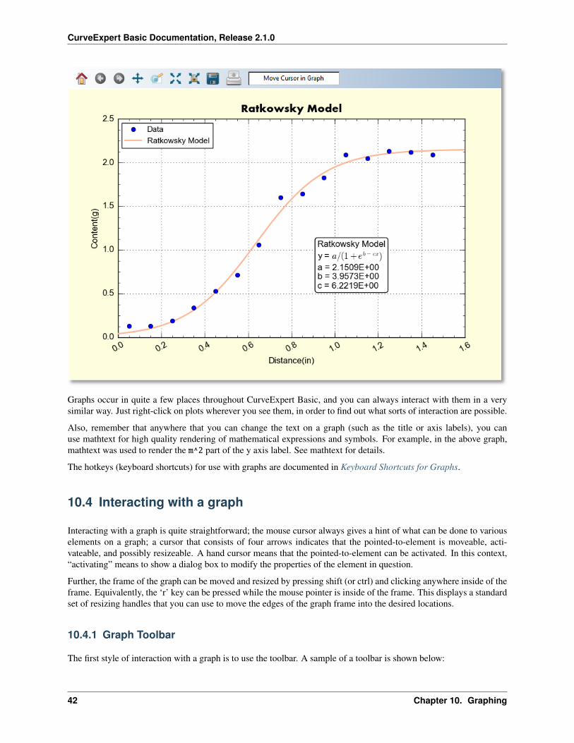
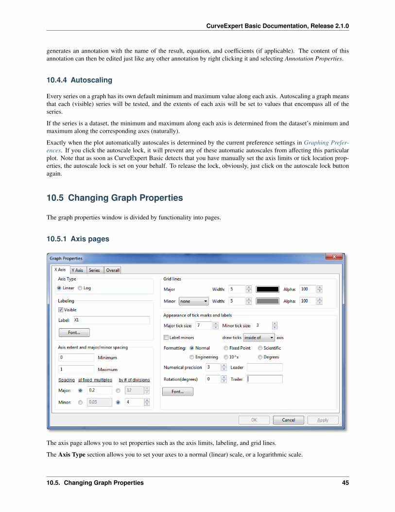
The graphing area is divided into two primary portions; the toolbar, which is situated along the top of a graphingarea, and the graph canvas, where the plot is drawn. The toolbar allows interactivity with the graph, such as panning,zooming, and autoscaling. Right clicking on the plot canvas shows the graphing menu, where you can customize itemson the plot like the axis labels, title, and the look of the graph. Also from this menu, you can print, copy to clipboard,or save your graph in one of many picture formats. An example of a graph is shown below:
41
CurveExpert Basic Documentation, Release 2.1.0
Graphs occur in quite a few places throughout CurveExpert Basic, and you can always interact with them in a verysimilar way. Just right-click on plots wherever you see them, in order to find out what sorts of interaction are possible.
Also, remember that anywhere that you can change the text on a graph (such as the title or axis labels), you canuse mathtext for high quality rendering of mathematical expressions and symbols. For example, in the above graph,mathtext was used to render the m^2 part of the y axis label. See mathtext for details.
The hotkeys (keyboard shortcuts) for use with graphs are documented in Keyboard Shortcuts for Graphs.
10.4 Interacting with a graph
Interacting with a graph is quite straightforward; the mouse cursor always gives a hint of what can be done to variouselements on a graph; a cursor that consists of four arrows indicates that the pointed-to-element is moveable, acti-vateable, and possibly resizeable. A hand cursor means that the pointed-to-element can be activated. In this context,“activating” means to show a dialog box to modify the properties of the element in question.
Further, the frame of the graph can be moved and resized by pressing shift (or ctrl) and clicking anywhere inside of theframe. Equivalently, the ‘r’ key can be pressed while the mouse pointer is inside of the frame. This displays a standardset of resizing handles that you can use to move the edges of the graph frame into the desired locations.
10.4.1 Graph Toolbar
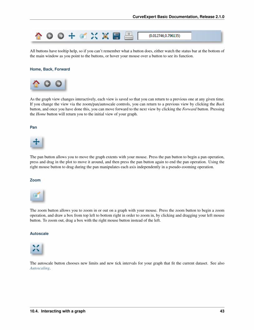
The first style of interaction with a graph is to use the toolbar. A sample of a toolbar is shown below:
42 Chapter 10. Graphing
CurveExpert Basic Documentation, Release 2.1.0
All buttons have tooltip help, so if you can’t remember what a button does, either watch the status bar at the bottom ofthe main window as you point to the buttons, or hover your mouse over a button to see its function.
Home, Back, Forward
As the graph view changes interactively, each view is saved so that you can return to a previous one at any given time.If you change the view via the zoom/pan/autoscale controls, you can return to a previous view by clicking the Backbutton, and once you have done this, you can move forward to the next view by clicking the Forward button. Pressingthe Home button will return you to the initial view of your graph.
Pan
The pan button allows you to move the graph extents with your mouse. Press the pan button to begin a pan operation,press and drag in the plot to move it around, and then press the pan button again to end the pan operation. Using theright mouse button to drag during the pan manipulates each axis independently in a pseudo-zooming operation.
Zoom
The zoom button allows you to zoom in or out on a graph with your mouse. Press the zoom button to begin a zoomoperation, and draw a box from top left to bottom right in order to zoom in, by clicking and dragging your left mousebutton. To zoom out, drag a box with the right mouse button instead of the left.
Autoscale
The autoscale button chooses new limits and new tick intervals for your graph that fit the current dataset. See alsoAutoscaling.
10.4. Interacting with a graph 43
CurveExpert Basic Documentation, Release 2.1.0
Autoscale lock
CurveExpert Basic will automatically autoscale your plot as data or results are added, changed, or removed. Thisis done according to Graphing Preferences. If you click the autoscale lock, it will prevent any of these automaticautoscales from affecting this particular plot. Note that as soon as CurveExpert Basic detects that you have manuallyset the axis limits or tick location properties (see Axis pages), the autoscale lock is set on your behalf. To release thelock, obviously, just click on the autoscale lock button again.
Save
The save button allows you to save your graph in a variety of picture formats. Pressing this button shows a file chooser,so that you can select the file type and where to save the graph. See Saving graphs for more information, includingsupported image formats.
The print button allows you to quickly output a hardcopy of the currently visible graph.
Locator
The locator always reports the location of your mouse, in data coordinates.
10.4.2 Dragging Elements on Graphs
Items like legends and graph titles are all draggable; meaning that they can be moved directly via interaction with themouse. If any of these elements are not where you desire them be, simply click and drag it to the desired position.
10.4.3 Picking
If you point to a series on your graph, it will become highlighted. If you then double-click the mouse, a dialog willappear to allow you to change the properties of that series (color, marker style, etc.).
Further, if you right click on a series, you can also select Details in order to show the details for the underlyingdataset or result associated with that particular curve. When right-clicking on a curve, there is also the opportunityto automatically add an annotation with information about that particular curve’s result; choose Autoannotate. This
44 Chapter 10. Graphing
CurveExpert Basic Documentation, Release 2.1.0
generates an annotation with the name of the result, equation, and coefficients (if applicable). The content of thisannotation can then be edited just like any other annotation by right clicking it and selecting Annotation Properties.
10.4.4 Autoscaling
Every series on a graph has its own default minimum and maximum value along each axis. Autoscaling a graph meansthat each (visible) series will be tested, and the extents of each axis will be set to values that encompass all of theseries.
If the series is a dataset, the minimum and maximum along each axis is determined from the dataset’s minimum andmaximum along the corresponding axes (naturally).
Exactly when the plot automatically autoscales is determined by the current preference settings in Graphing Prefer-ences. If you click the autoscale lock, it will prevent any of these automatic autoscales from affecting this particularplot. Note that as soon as CurveExpert Basic detects that you have manually set the axis limits or tick location prop-erties, the autoscale lock is set on your behalf. To release the lock, obviously, just click on the autoscale lock buttonagain.
10.5 Changing Graph Properties
The graph properties window is divided by functionality into pages.
10.5.1 Axis pages
The axis page allows you to set properties such as the axis limits, labeling, and grid lines.
The Axis Type section allows you to set your axes to a normal (linear) scale, or a logarithmic scale.
10.5. Changing Graph Properties 45
CurveExpert Basic Documentation, Release 2.1.0
The Labeling section can be used to either hide the axis label, or specify the label itself. Also, the font and font colorof the axis label can be selected by pressing the Font button in this section.
The Axis extent and major/minor spacing section allows you to specify the minimum and maximum value of theaxis (determining its limits). To have your axis run in reverse, set the maximum of the axis less than the minimum.
The major and minor spacing can each be set in one of two ways: by a fixed amount of spacing between each tick, orby the number of divisions an interval is divided into. To select the kind of spacing, click the radio buttons under theat fixed multiples or by # of divisions column as desired. If at fixed multiples is chosen, each tick mark (either majoror minor) is set each time the multiple appears on the axis. For example, if the major ticks are set at fixed multiplesof 0.2, there will be a major tick at -0.2, 0, 0.2, 0.4, etc. If by # of divisions is chosen, the ticks are placed such thatthe appropriate interval (the entire axis in the case of minor ticks, and the interval between two majors in the case ofmajor ticks) is divided into the specified number of parts. For example, if the minor ticks are set to a # of divisions of4, there should be four intervals between each major tick (which means that three minors will be visible).
The Grid Lines section allows you to specify the line style, line width, color, and transparency (alpha) of both themajor and minor grid lines.
The Appearance of tick marks and labels section is where the size and style of tick marks, the font and color ofthe tick mark labels, and the numerical format of the tick mark labels can be specified. The Major/Minor tick sizedetermines how large the markers are that are placed at each tick, in points. Also, the Draw ticks inside of axis settingdetermines if these tick marks are placed completely inside, outside, or across the axis. Label minors determineswhether or not text labels are placed at each minor demarcation (most useful for log scaled plots).
The format of the tick mark labels is determined by the combination of the Formatting setting and the Numericalprecision setting. Formatting can be set to normal for a generic style of numerical formatting, fixed point, scientific,engineering, 10^x, or degrees. In all cases except for normal formatting and 10^x, the Numerical precision fielddetermines exactly how many places are shown after the decimal in the label.
• Normal: a generic style of formatting that lets the software determine best appearance. e.g. 10245.1234
• Fixed point: exactly like normal formatting, except that the numerical precision is honored. e.g. 10245.1(coupled with a numerical precision of 1)
• Scientific: a mantissa followed by an exponent. e.g. 1.02e4 (coupled with a precision of 2)
• Engineering: a mantissa followed by an exponent that is a power of 3. e.g. 10.25e3 (coupled with a precision of2)
• 10^x: most useful for log scale plots, where the user desires to display the number on the axis as 10 raised tothe appropriate exponent. e.g. 102
• Degrees: most useful when the user desires to display a number in radians as a number in degrees. e.g. 60∘
(coupled with a precision of 0)
Any axis tick label can be preceded or followed by customized text (including mathtext) as you specify. For text toappear before each axis label, place the text in the Leader field; for text to appear after each axis label, place the textin the Trailer field. By default, no text appears before or after the axis tick label. Examples of common usage of thisfeature are to place a dollar sign in front of the numbers to indicate currency, or units after the label.
Finally, the set of tick labels can be rotated by a certain number of degrees, which is also configurable in this sectionvia the Rotation setting.
46 Chapter 10. Graphing
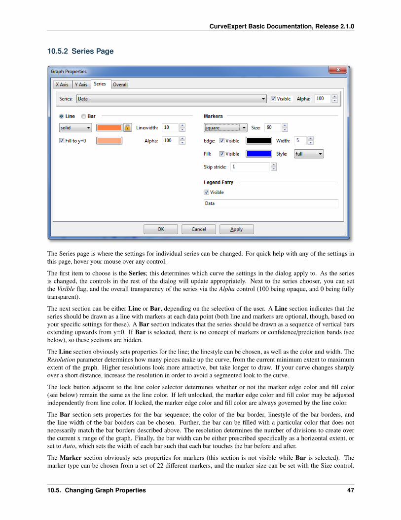
CurveExpert Basic Documentation, Release 2.1.0
10.5.2 Series Page
The Series page is where the settings for individual series can be changed. For quick help with any of the settings inthis page, hover your mouse over any control.
The first item to choose is the Series; this determines which curve the settings in the dialog apply to. As the seriesis changed, the controls in the rest of the dialog will update appropriately. Next to the series chooser, you can setthe Visible flag, and the overall transparency of the series via the Alpha control (100 being opaque, and 0 being fullytransparent).
The next section can be either Line or Bar, depending on the selection of the user. A Line section indicates that theseries should be drawn as a line with markers at each data point (both line and markers are optional, though, based onyour specific settings for these). A Bar section indicates that the series should be drawn as a sequence of vertical barsextending upwards from y=0. If Bar is selected, there is no concept of markers or confidence/prediction bands (seebelow), so these sections are hidden.
The Line section obviously sets properties for the line; the linestyle can be chosen, as well as the color and width. TheResolution parameter determines how many pieces make up the curve, from the current minimum extent to maximumextent of the graph. Higher resolutions look more attractive, but take longer to draw. If your curve changes sharplyover a short distance, increase the resolution in order to avoid a segmented look to the curve.
The lock button adjacent to the line color selector determines whether or not the marker edge color and fill color(see below) remain the same as the line color. If left unlocked, the marker edge color and fill color may be adjustedindependently from line color. If locked, the marker edge color and fill color are always governed by the line color.
The Bar section sets properties for the bar sequence; the color of the bar border, linestyle of the bar borders, andthe line width of the bar borders can be chosen. Further, the bar can be filled with a particular color that does notnecessarily match the bar borders described above. The resolution determines the number of divisions to create overthe current x range of the graph. Finally, the bar width can be either prescribed specifically as a horizontal extent, orset to Auto, which sets the width of each bar such that each bar touches the bar before and after.
The Marker section obviously sets properties for markers (this section is not visible while Bar is selected). Themarker type can be chosen from a set of 22 different markers, and the marker size can be set with the Size control.
10.5. Changing Graph Properties 47
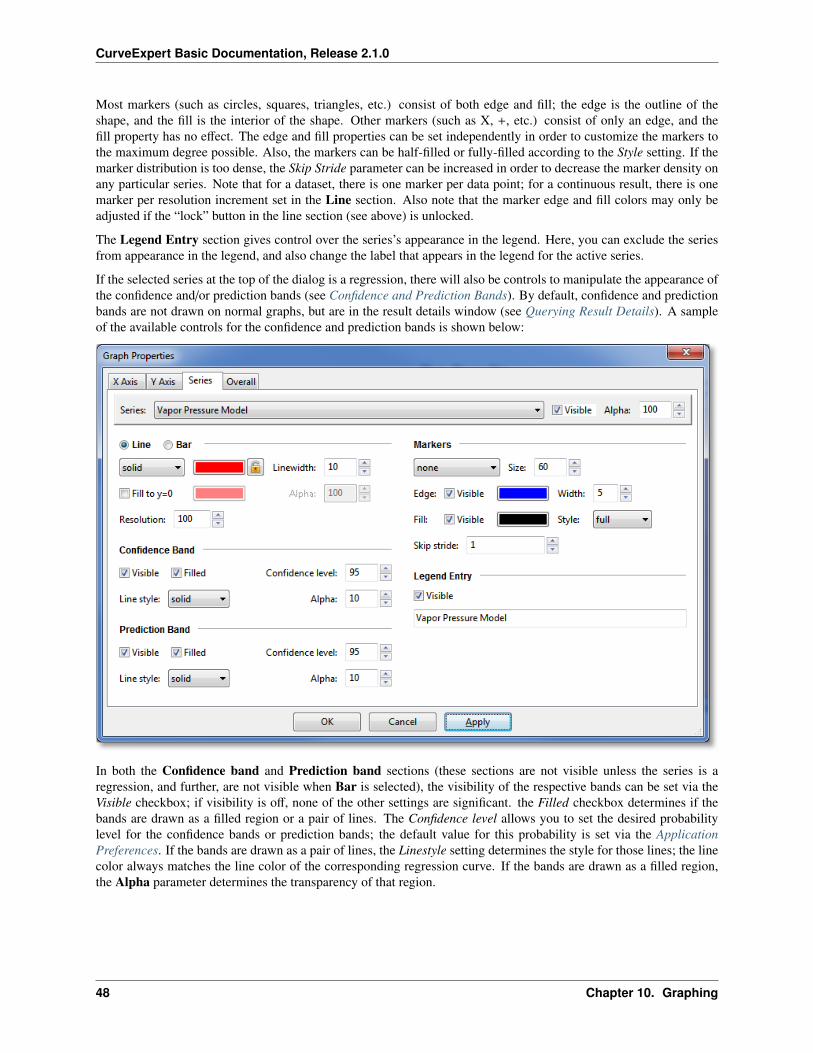
CurveExpert Basic Documentation, Release 2.1.0
Most markers (such as circles, squares, triangles, etc.) consist of both edge and fill; the edge is the outline of theshape, and the fill is the interior of the shape. Other markers (such as X, +, etc.) consist of only an edge, and thefill property has no effect. The edge and fill properties can be set independently in order to customize the markers tothe maximum degree possible. Also, the markers can be half-filled or fully-filled according to the Style setting. If themarker distribution is too dense, the Skip Stride parameter can be increased in order to decrease the marker density onany particular series. Note that for a dataset, there is one marker per data point; for a continuous result, there is onemarker per resolution increment set in the Line section. Also note that the marker edge and fill colors may only beadjusted if the “lock” button in the line section (see above) is unlocked.
The Legend Entry section gives control over the series’s appearance in the legend. Here, you can exclude the seriesfrom appearance in the legend, and also change the label that appears in the legend for the active series.
If the selected series at the top of the dialog is a regression, there will also be controls to manipulate the appearance ofthe confidence and/or prediction bands (see Confidence and Prediction Bands). By default, confidence and predictionbands are not drawn on normal graphs, but are in the result details window (see Querying Result Details). A sampleof the available controls for the confidence and prediction bands is shown below:
In both the Confidence band and Prediction band sections (these sections are not visible unless the series is aregression, and further, are not visible when Bar is selected), the visibility of the respective bands can be set via theVisible checkbox; if visibility is off, none of the other settings are significant. the Filled checkbox determines if thebands are drawn as a filled region or a pair of lines. The Confidence level allows you to set the desired probabilitylevel for the confidence bands or prediction bands; the default value for this probability is set via the ApplicationPreferences. If the bands are drawn as a pair of lines, the Linestyle setting determines the style for those lines; the linecolor always matches the line color of the corresponding regression curve. If the bands are drawn as a filled region,the Alpha parameter determines the transparency of that region.
48 Chapter 10. Graphing
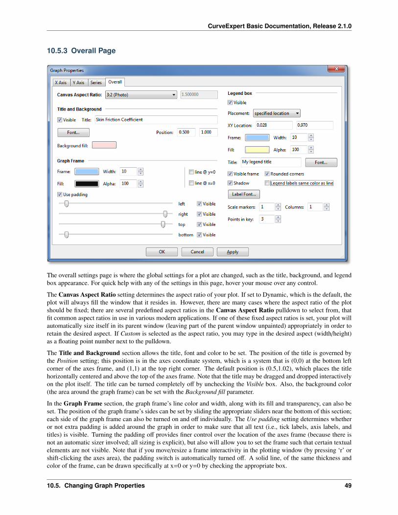
CurveExpert Basic Documentation, Release 2.1.0
10.5.3 Overall Page
The overall settings page is where the global settings for a plot are changed, such as the title, background, and legendbox appearance. For quick help with any of the settings in this page, hover your mouse over any control.
The Canvas Aspect Ratio setting determines the aspect ratio of your plot. If set to Dynamic, which is the default, theplot will always fill the window that it resides in. However, there are many cases where the aspect ratio of the plotshould be fixed; there are several predefined aspect ratios in the Canvas Aspect Ratio pulldown to select from, thatfit common aspect ratios in use in various modern applications. If one of these fixed aspect ratios is set, your plot willautomatically size itself in its parent window (leaving part of the parent window unpainted) appropriately in order toretain the desired aspect. If Custom is selected as the aspect ratio, you may type in the desired aspect (width/height)as a floating point number next to the pulldown.
The Title and Background section allows the title, font and color to be set. The position of the title is governed bythe Position setting; this position is in the axes coordinate system, which is a system that is (0,0) at the bottom leftcorner of the axes frame, and (1,1) at the top right corner. The default position is (0.5,1.02), which places the titlehorizontally centered and above the top of the axes frame. Note that the title may be dragged and dropped interactivelyon the plot itself. The title can be turned completely off by unchecking the Visible box. Also, the background color(the area around the graph frame) can be set with the Background fill parameter.
In the Graph Frame section, the graph frame’s line color and width, along with its fill and transparency, can also beset. The position of the graph frame’s sides can be set by sliding the appropriate sliders near the bottom of this section;each side of the graph frame can also be turned on and off individually. The Use padding setting determines whetheror not extra padding is added around the graph in order to make sure that all text (i.e., tick labels, axis labels, andtitles) is visible. Turning the padding off provides finer control over the location of the axes frame (because there isnot an automatic sizer involved; all sizing is explicit), but also will allow you to set the frame such that certain textualelements are not visible. Note that if you move/resize a frame interactivity in the plotting window (by pressing ‘r’ orshift-clicking the axes area), the padding switch is automatically turned off. A solid line, of the same thickness andcolor of the frame, can be drawn specifically at x=0 or y=0 by checking the appropriate box.
10.5. Changing Graph Properties 49
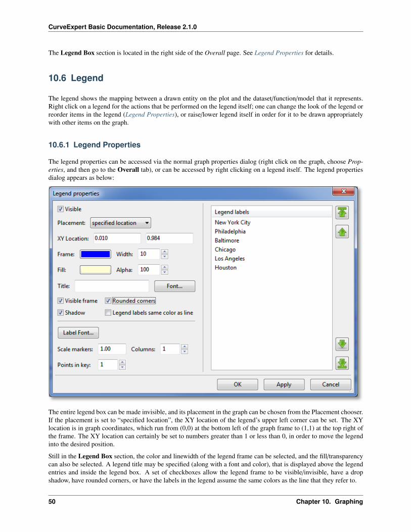
CurveExpert Basic Documentation, Release 2.1.0
The Legend Box section is located in the right side of the Overall page. See Legend Properties for details.
10.6 Legend
The legend shows the mapping between a drawn entity on the plot and the dataset/function/model that it represents.Right click on a legend for the actions that be performed on the legend itself; one can change the look of the legend orreorder items in the legend (Legend Properties), or raise/lower legend itself in order for it to be drawn appropriatelywith other items on the graph.
10.6.1 Legend Properties
The legend properties can be accessed via the normal graph properties dialog (right click on the graph, choose Prop-erties, and then go to the Overall tab), or can be accessed by right clicking on a legend itself. The legend propertiesdialog appears as below:
The entire legend box can be made invisible, and its placement in the graph can be chosen from the Placement chooser.If the placement is set to “specified location”, the XY location of the legend’s upper left corner can be set. The XYlocation is in graph coordinates, which run from (0,0) at the bottom left of the graph frame to (1,1) at the top right ofthe frame. The XY location can certainly be set to numbers greater than 1 or less than 0, in order to move the legendinto the desired position.
Still in the Legend Box section, the color and linewidth of the legend frame can be selected, and the fill/transparencycan also be selected. A legend title may be specified (along with a font and color), that is displayed above the legendentries and inside the legend box. A set of checkboxes allow the legend frame to be visible/invisible, have a dropshadow, have rounded corners, or have the labels in the legend assume the same colors as the line that they refer to.
50 Chapter 10. Graphing
CurveExpert Basic Documentation, Release 2.1.0
At the bottom of the Legend Box section, the font and color of the legend labels can be selected. If markers needto be made smaller or larger in the legend, a Scale markers setting takes care of this. To lay your legend out in amulticolumn format, increase the number of columns in the Columns setting. To include more than one marker in alegend key, increase the Points in key setting.
10.6.2 Legend label editing
Legend labels may be changed in the Legend labels section, by clicking an already-selected label. The label willbecome editable, and you can change the text to whatever is desired. Remember that mathtext can be used in a legendlabel as well. Also, the label can be made blank so that the series does not appear in the legend. Editing a label in thismanner is exactly the same as doing so via the Series Page in the Graph Properties dialog.
10.6.3 Legend Ordering
The order of the series in of a legend can be changed by selecting the desired series’s legend label in the Legend labelssection, and pressing the appropriate arrow buttons to arrange the ordering of the series. The topmost arrow buttonmoves the selected series to the top; while the bottommost arrow button moves the selected series to the bottom. Theinner two arrow buttons move the selected series up or down by one slot as appropriate.
The ordering of items in the legend also has another important role: it determines the order in which each series isdrawn in the graph. So, if you would like a particular series to be drawn on top, move it to the front in the legendordering. Series are drawn in reverse order as the legend ordering, which means that the item appearing on top of thelegend order will also appear on top of other series in the graph.
10.7 Saving graphs
To save a graph, either choose the Save button in the graph toolbar, or right click the graph and select Save. A filechooser will appear that allows you to select the location and filename of the graph to be saved, and the format of thepicture file to be saved. For image (raster) files, supported filetypes are:
• portable network graphics (PNG)
• JPEG
• TIFF
• raw RGBA bitmaps (RGBA or RAW)
Supported vector graphics file formats are:
• scalable vector graphics (SVG)
• enhanced metafiles (EMF)
• encapsulated postscript (EPS)
• postscript (PS)
• portable document format (PDF)
Of these formats, the PNG format is the most common for raster-type images, and SVG is most common for vectorgraphics. A PNG file can be read by any graphics application, and by applications such as Microsoft Word andPowerpoint. SVG files can be read by computer illustration software, such as Adobe Illustrator or Inkscape. It shouldbe noted that an SVG file written by CurveExpert Basic retains all object information, so you can add or removeelements from the graph after-the-fact with an illustration package, if desired.
10.7. Saving graphs 51
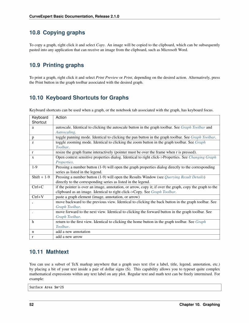
CurveExpert Basic Documentation, Release 2.1.0
10.8 Copying graphs
To copy a graph, right click it and select Copy. An image will be copied to the clipboard, which can be subsequentlypasted into any application that can receive an image from the clipboard, such as Microsoft Word.
10.9 Printing graphs
To print a graph, right click it and select Print Preview or Print, depending on the desired action. Alternatively, pressthe Print button in the graph toolbar associated with the desired graph.
10.10 Keyboard Shortcuts for Graphs
Keyboard shortcuts can be used when a graph, or the notebook tab associated with the graph, has keyboard focus.
KeyboardShortcut
Action
a autoscale. Identical to clicking the autoscale button in the graph toolbar. See Graph Toolbar andAutoscaling.
p toggle panning mode. Identical to clicking the pan button in the graph toolbar. See Graph Toolbar.z toggle zooming mode. Identical to clicking the zoom button in the graph toolbar. See Graph
Toolbar.r resize the graph frame interactively (pointer must be over the frame when r is pressed).x Open context sensitive properties dialog. Identical to right click->Properties. See Changing Graph
Properties.1-9 Pressing a number button (1-9) will open the graph properties dialog directly to the corresponding
series as listed in the legend.Shift + 1-9 Pressing a number button (1-9) will open the Results Window (see Querying Result Details)
directly to the corresponding series as listed in the legend.Ctrl+C if the pointer is over an image, annotation, or arrow, copy it; if over the graph, copy the graph to the
clipboard as an image. Identical to right click->Copy. See Graph Toolbar.Ctrl+V paste a graph element (image, annotation, or arrow), move backward to the previous view. Identical to clicking the back button in the graph toolbar. See
Graph Toolbar.. move forward to the next view. Identical to clicking the forward button in the graph toolbar. See
Graph Toolbar.h return to the first view. Identical to clicking the home button in the graph toolbar. See Graph
Toolbar.n add a new annotationr add a new arrow
10.11 Mathtext
You can use a subset of TeX markup anywhere that a graph uses text (for a label, title, legend, annotation, etc.)by placing a bit of your text inside a pair of dollar signs ($). This capability allows you to typeset quite complexmathematical expressions within any text label on any plot. Regular text and math text can be freely intermixed. Forexample:
Surface Area $m^2$
52 Chapter 10. Graphing
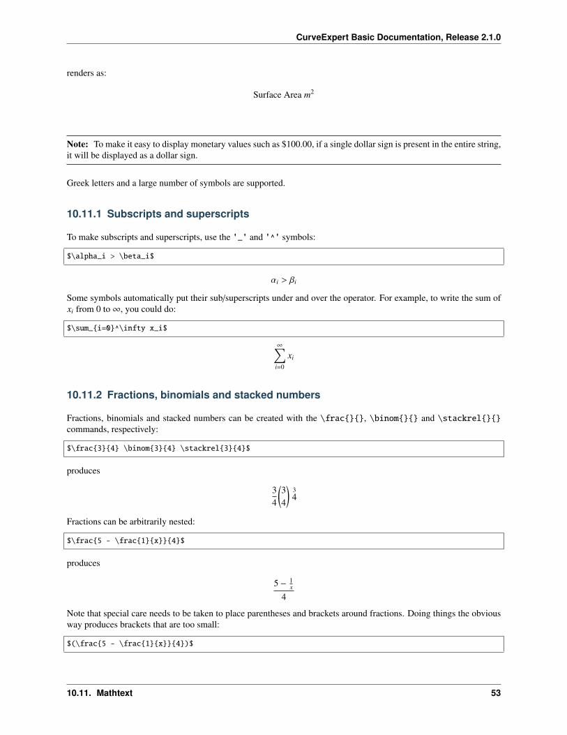
CurveExpert Basic Documentation, Release 2.1.0
renders as:
Surface Area m2
Note: To make it easy to display monetary values such as $100.00, if a single dollar sign is present in the entire string,it will be displayed as a dollar sign.
Greek letters and a large number of symbols are supported.
10.11.1 Subscripts and superscripts
To make subscripts and superscripts, use the '_' and '^' symbols:
$\alpha_i > \beta_i$
αi > βi
Some symbols automatically put their sub/superscripts under and over the operator. For example, to write the sum ofxi from 0 to∞, you could do:
$\sum_i=0^\infty x_i$
∞∑i=0
xi
10.11.2 Fractions, binomials and stacked numbers
Fractions, binomials and stacked numbers can be created with the \frac, \binom and \stackrelcommands, respectively:
$\frac34 \binom34 \stackrel34$
produces
34
(34
)34
Fractions can be arbitrarily nested:
$\frac5 - \frac1x4$
produces
5 − 1x
4
Note that special care needs to be taken to place parentheses and brackets around fractions. Doing things the obviousway produces brackets that are too small:
$(\frac5 - \frac1x4)$
10.11. Mathtext 53
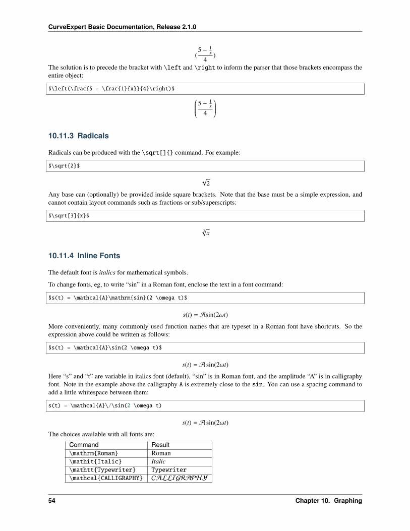
CurveExpert Basic Documentation, Release 2.1.0
(5 − 1
x
4)
The solution is to precede the bracket with \left and \right to inform the parser that those brackets encompass theentire object:
$\left(\frac5 - \frac1x4\right)$ ⎛⎜⎜⎜⎜⎜⎝5 − 1x
4
⎞⎟⎟⎟⎟⎟⎠10.11.3 Radicals
Radicals can be produced with the \sqrt[] command. For example:
$\sqrt2$
√2
Any base can (optionally) be provided inside square brackets. Note that the base must be a simple expression, andcannot contain layout commands such as fractions or sub/superscripts:
$\sqrt[3]x$
3√x
10.11.4 Inline Fonts
The default font is italics for mathematical symbols.
To change fonts, eg, to write “sin” in a Roman font, enclose the text in a font command:
$s(t) = \mathcalA\mathrmsin(2 \omega t)$
s(t) = 𝒜sin(2ωt)
More conveniently, many commonly used function names that are typeset in a Roman font have shortcuts. So theexpression above could be written as follows:
$s(t) = \mathcalA\sin(2 \omega t)$
s(t) = 𝒜 sin(2ωt)
Here “s” and “t” are variable in italics font (default), “sin” is in Roman font, and the amplitude “A” is in calligraphyfont. Note in the example above the calligraphy A is extremely close to the sin. You can use a spacing command toadd a little whitespace between them:
s(t) = \mathcalA\/\sin(2 \omega t)
s(t) = 𝒜 sin(2ωt)
The choices available with all fonts are:
Command Result\mathrmRoman Roman\mathitItalic Italic\mathttTypewriter Typewriter
\mathcalCALLIGRAPHY 𝒞𝒜ℒℒℐ𝒢ℛ𝒜𝒫ℋ𝒴
54 Chapter 10. Graphing
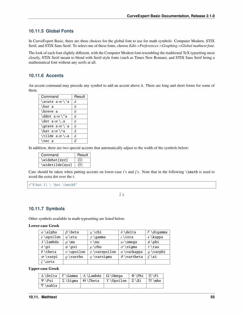
CurveExpert Basic Documentation, Release 2.1.0
10.11.5 Global Fonts
In CurveExpert Basic, there are three choices for the global font to use for math symbols: Computer Modern, STIXSerif, and STIX Sans Serif. To select one of these fonts, choose Edit->Preferences->Graphing->Global mathtext font.
The look of each font slightly different, with the Computer Modern font resembling the traditional TeX typsetting mostclosely, STIX Serif meant to blend with Serif-style fonts (such as Times New Roman), and STIX Sans Serif being amathematical font without any serifs at all.
10.11.6 Accents
An accent command may precede any symbol to add an accent above it. There are long and short forms for some ofthem.
Command Result\acute a or \'a a\bar a a\breve a a\ddot a or \"a a\dot a or \.a a\grave a or \`a a\hat a or \^a a\tilde a or \~a a\vec a ~a
In addition, there are two special accents that automatically adjust to the width of the symbols below:
Command Result\widehatxyz xyz\widetildexyz xyz
Care should be taken when putting accents on lower-case i’s and j’s. Note that in the following \imath is used toavoid the extra dot over the i:
r"$\hat i\ \ \hat \imath$"
i ı
10.11.7 Symbols
Other symbols available in math typesetting are listed below.
Lower-case Greekα \alpha β \beta χ \chi δ \delta z \digammaε \epsilon η \eta γ \gamma ι \iota κ \kappaλ \lambda µ \mu ν \nu ω \omega φ \phiπ \pi ψ \psi ρ \rho σ \sigma τ \tauθ \theta υ \upsilon ε \varepsilon κ \varkappa ϕ \varphi$ \varpi % \varrho ς \varsigma ϑ \vartheta ξ \xiζ \zeta
Upper-case Greek
∆ \Delta Γ \Gamma Λ \Lambda Ω \Omega Φ \Phi Π \PiΨ \Psi Σ \Sigma Θ \Theta Υ \Upsilon Ξ \Xi f \mho∇ \nabla
10.11. Mathtext 55
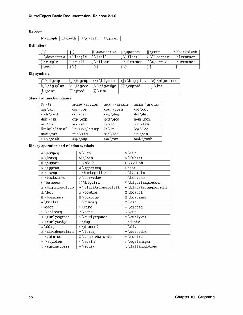
CurveExpert Basic Documentation, Release 2.1.0
Hebrew
ℵ \aleph i \beth k \daleth ג \gimel
Delimiters/ / [ [ ⇓ \Downarrow ⇑ \Uparrow ‖ \Vert ∖ \backslash↓ \downarrow ⟨ \langle ⌈ \lceil ⌊ \lfloor x \llcorner y \lrcorner⟩ \rangle ⌉ \rceil ⌋ \rfloor p \ulcorner ↑ \uparrow q \urcorner| \vert \ ‖ \| \ ] ] | |
Big symbols⋂\bigcap
⋃\bigcup
⨀\bigodot
⨁\bigoplus
⨂\bigotimes⨄
\biguplus⋁\bigvee
⋀\bigwedge
∐\coprod
∫\int∮
\oint∏\prod
∑\sum
Standard function namesPr \Pr arccos \arccos arcsin \arcsin arctan \arctanarg \arg cos \cos cosh \cosh cot \cotcoth \coth csc \csc deg \deg det \detdim \dim exp \exp gcd \gcd hom \hominf \inf ker \ker lg \lg lim \limlim inf \liminf lim sup \limsup ln \ln log \logmax \max min \min sec \sec sin \sinsinh \sinh sup \sup tan \tan tanh \tanh
Binary operation and relation symbols
m \Bumpeq e \Cap d \Cup+ \Doteq Z \Join b \Subsetc \Supset \Vdash \Vvdash≈ \approx u \approxeq * \ast≍ \asymp \backepsilon v \backsimw \backsimeq Z \barwedge ∵ \becauseG \between \bigcirc \bigtriangledown \bigtriangleup J \blacktriangleleft I \blacktriangleright⊥ \bot ./ \bowtie \boxdot \boxminus \boxplus \boxtimes∙ \bullet l \bumpeq ∩ \cap· \cdot ∘ \circ $ \circeqD \coloneq \cong ∪ \cup2 \curlyeqprec 3 \curlyeqsucc g \curlyveef \curlywedge † \dag ⊣ \dashv‡ \ddag \diamond ÷ \div> \divideontimes \doteq + \doteqdotu \dotplus [ \doublebarwedge P \eqcircE \eqcolon h \eqsim 1 \eqslantgtr0 \eqslantless ≡ \equiv ; \fallingdotseq
56 Chapter 10. Graphing
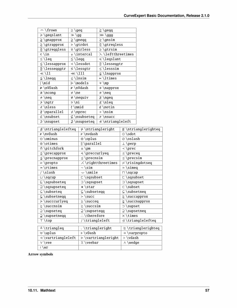
CurveExpert Basic Documentation, Release 2.1.0
_ \frown ≥ \geq = \geqq> \geqslant ≫ \gg ≫ \ggg \gnapprox \gneqq \gnsim' \gtrapprox m \gtrdot R \gtreqlessT \gtreqqless ≷ \gtrless & \gtrsim∈ \in ᵀ \intercal h \leftthreetimes≤ \leq 5 \leqq 6 \leqslant/ \lessapprox l \lessdot Q \lesseqgtrS \lesseqqgtr ≶ \lessgtr . \lesssim≪ \ll ≪ \lll \lnapprox \lneqq \lnsim n \ltimes| \mid |= \models ∓ \mp3 \nVDash 1 \nVdash 0 \napprox \ncong , \ne , \neq, \neq . \nequiv \ngeq≯ \ngtr ∋ \ni \nleq≮ \nless - \nmid < \notin∦ \nparallel ⊀ \nprec / \nsim1 \nsubset * \nsubseteq \nsucc2 \nsupset + \nsupseteq 6 \ntriangleleft
5 \ntrianglelefteq 7 \ntriangleright 4 \ntrianglerighteq2 \nvDash 0 \nvdash ⊙ \odot⊖ \ominus ⊕ \oplus ⊘ \oslash⊗ \otimes ‖ \parallel ⊥ \perpt \pitchfork ± \pm ≺ \precv \precapprox 4 \preccurlyeq ⪯ \preceq \precnapprox \precnsim - \precsim∝ \propto i \rightthreetimes : \risingdotseqo \rtimes ∼ \sim ≃ \simeq/ \slash ^ \smile ⊓ \sqcap⊔ \sqcup @ \sqsubset @ \sqsubset⊑ \sqsubseteq A \sqsupset A \sqsupset⊒ \sqsupseteq ? \star ⊂ \subset⊆ \subseteq j \subseteqq ( \subsetneq$ \subsetneqq ≻ \succ w \succapprox< \succcurlyeq ⪰ \succeq \succnapprox \succnsim % \succsim ⊃ \supset⊇ \supseteq k \supseteqq ) \supsetneq% \supsetneqq ∴ \therefore × \times⊤ \top / \triangleleft E \trianglelefteq
, \triangleq . \triangleright D \trianglerighteq⊎ \uplus \vDash ∝ \varproptoC \vartriangleleft B \vartriangleright ⊢ \vdash∨ \vee Y \veebar ∧ \wedge≀ \wr
Arrow symbols
10.11. Mathtext 57
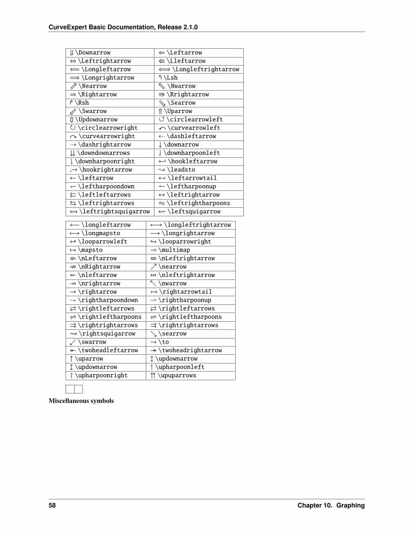
CurveExpert Basic Documentation, Release 2.1.0
⇓ \Downarrow ⇐ \Leftarrow⇔ \Leftrightarrow W \Lleftarrow⇐= \Longleftarrow ⇐⇒ \Longleftrightarrow=⇒ \Longrightarrow \Lsht \Nearrow v \Nwarrow⇒ \Rightarrow V \Rrightarrow \Rsh u \Searroww \Swarrow ⇑ \Uparrow \Updownarrow \circlearrowleft \circlearrowright x \curvearrowlefty \curvearrowright c \dashleftarrowd \dashrightarrow ↓ \downarrow \downdownarrows \downharpoonleft \downharpoonright ← \hookleftarrow→ \hookrightarrow \leadsto← \leftarrow \leftarrowtail \leftharpoondown \leftharpoonup⇔ \leftleftarrows ↔ \leftrightarrow \leftrightarrows \leftrightharpoons! \leftrightsquigarrow f \leftsquigarrow
←− \longleftarrow ←→ \longleftrightarrow↦−→ \longmapsto −→ \longrightarrow" \looparrowleft # \looparrowright↦→ \mapsto ( \multimap: \nLeftarrow < \nLeftrightarrow; \nRightarrow \nearrow8 \nleftarrow = \nleftrightarrow9 \nrightarrow \nwarrow→ \rightarrow \rightarrowtail \rightharpoondown \rightharpoonup \rightleftarrows \rightleftarrows \rightleftharpoons \rightleftharpoons⇒ \rightrightarrows ⇒ \rightrightarrows \rightsquigarrow \searrow \swarrow → \to \twoheadleftarrow \twoheadrightarrow↑ \uparrow \updownarrow \updownarrow \upharpoonleft \upharpoonright \upuparrows
Miscellaneous symbols
58 Chapter 10. Graphing
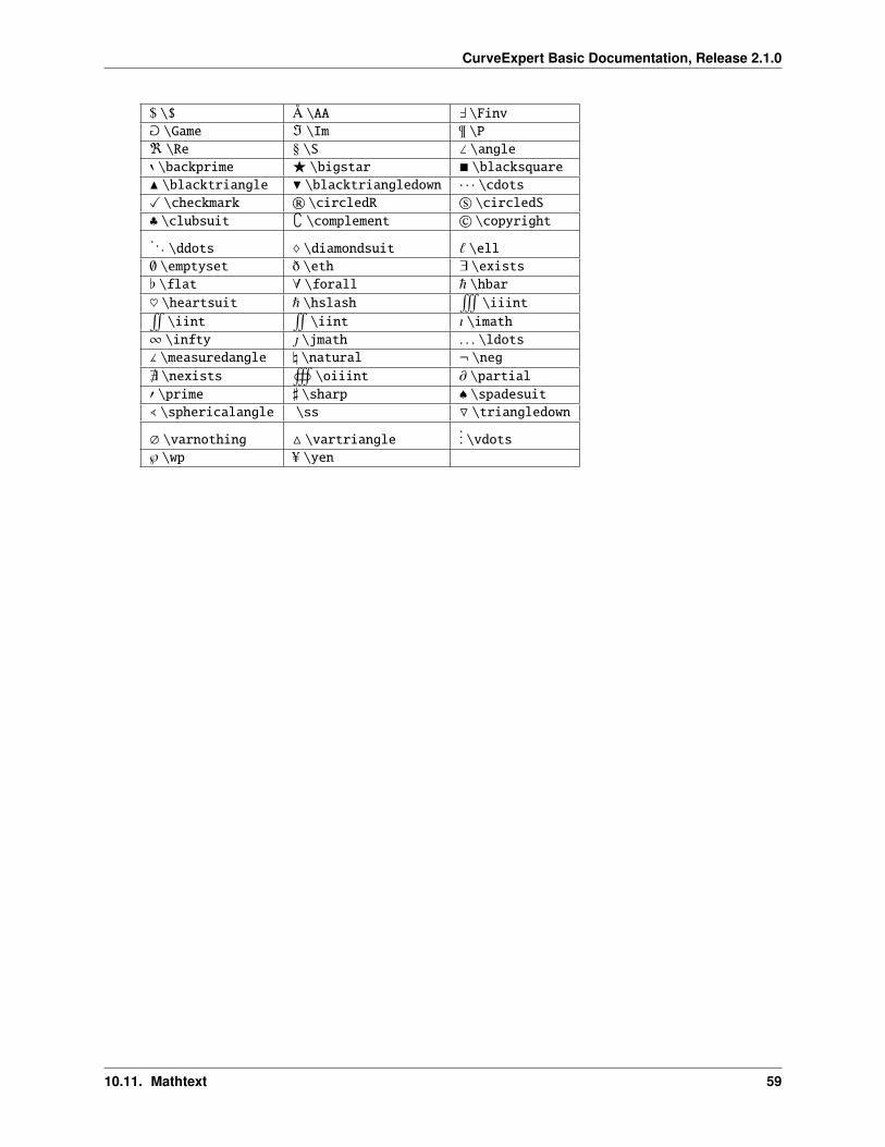
CurveExpert Basic Documentation, Release 2.1.0
$ \$ Å \AA ` \Finva \Game ℑ \Im ¶ \Pℜ \Re S \S ∠ \angle8 \backprime F \bigstar \blacksquareN \blacktriangle H \blacktriangledown · · · \cdotsX \checkmark r \circledR s \circledS♣ \clubsuit \complement © \copyright. . . \ddots \diamondsuit ` \ell∅ \emptyset ð \eth ∃ \exists[ \flat ∀ \forall ~ \hbar
\heartsuit \hslash#\iiint!
\iint!\iint ı \imath
∞ \infty \jmath . . . \ldots] \measuredangle \ \natural ¬ \neg
@ \nexists)\oiiint ∂ \partial
′ \prime ] \sharp ♠ \spadesuit^ \sphericalangle \ss O \triangledown
∅ \varnothing M \vartriangle... \vdots
℘ \wp U \yen
10.11. Mathtext 59

CurveExpert Basic Documentation, Release 2.1.0
60 Chapter 10. Graphing
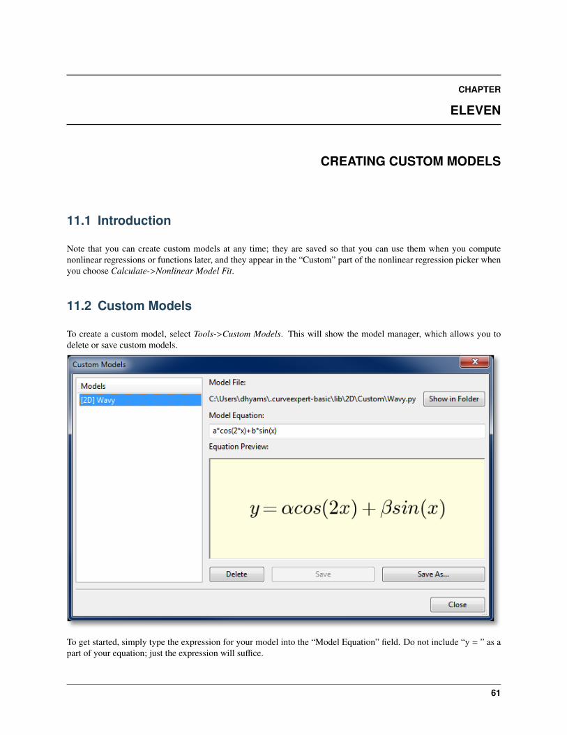
CHAPTER
ELEVEN
CREATING CUSTOM MODELS
11.1 Introduction
Note that you can create custom models at any time; they are saved so that you can use them when you computenonlinear regressions or functions later, and they appear in the “Custom” part of the nonlinear regression picker whenyou choose Calculate->Nonlinear Model Fit.
11.2 Custom Models
To create a custom model, select Tools->Custom Models. This will show the model manager, which allows you todelete or save custom models.
To get started, simply type the expression for your model into the “Model Equation” field. Do not include “y = ” as apart of your equation; just the expression will suffice.
61
CurveExpert Basic Documentation, Release 2.1.0
As you type, CurveExpert Basic will guess how to render your equation, even converting Greek letters into the appro-priate representation. The Equation Preview (see Equation Display) shows how your equation will render in Curve-Expert. Note that its guess is not adjustable in CurveExpert Basic; in CurveExpert Pro, the advanced code editor canbe used to adjust this. Usually the equation rendering is reasonable and correct, but in those cases in which it is not,remember that the rendering does not matter as far as the calculation and mathematics are concerned.
Once your model is written the way that you like, simply hit the Save or Save As button, depending your intent. Giveyour model a name, and your model will then appear in the list on the left, signifying that it is now available for usewithin CurveExpert Basic, when you choose to compute nonlinear regressions.
11.2.1 Mathematical Operations
Obviously, the standard arithmetic operations are supported. Multiplication is performed with a *, division with /,addition with +, and subtraction with -. Raising a quantity to a power is performed with either ^ or **, with the **notation being preferred. Grouping is performed with parentheses ().
11.2.2 Reserved Words
In any model, the independent variable is always denoted by x. This variable is a reserved word and should not beused as a parameter name in your model.
All mathematical functions supported by CurveExpert Basic, such as sin, cos, tan, exp, etc., are also reserved words.See Appendix A: Math Functions for a complete list of the mathematical functions supported.
Any other name that CurveExpert Basic sees in your model is treated as a parameter. This powerful feature letsyou name your parameters any name that you find appropriate, such that the model’s syntax carries meaning. Thus,names such as beta, my_long_parameter_name, and b are all legal parameter names. Note also that names are casesensitive; the parameter a is distinct from the parameter A, for example.
62 Chapter 11. Creating Custom Models
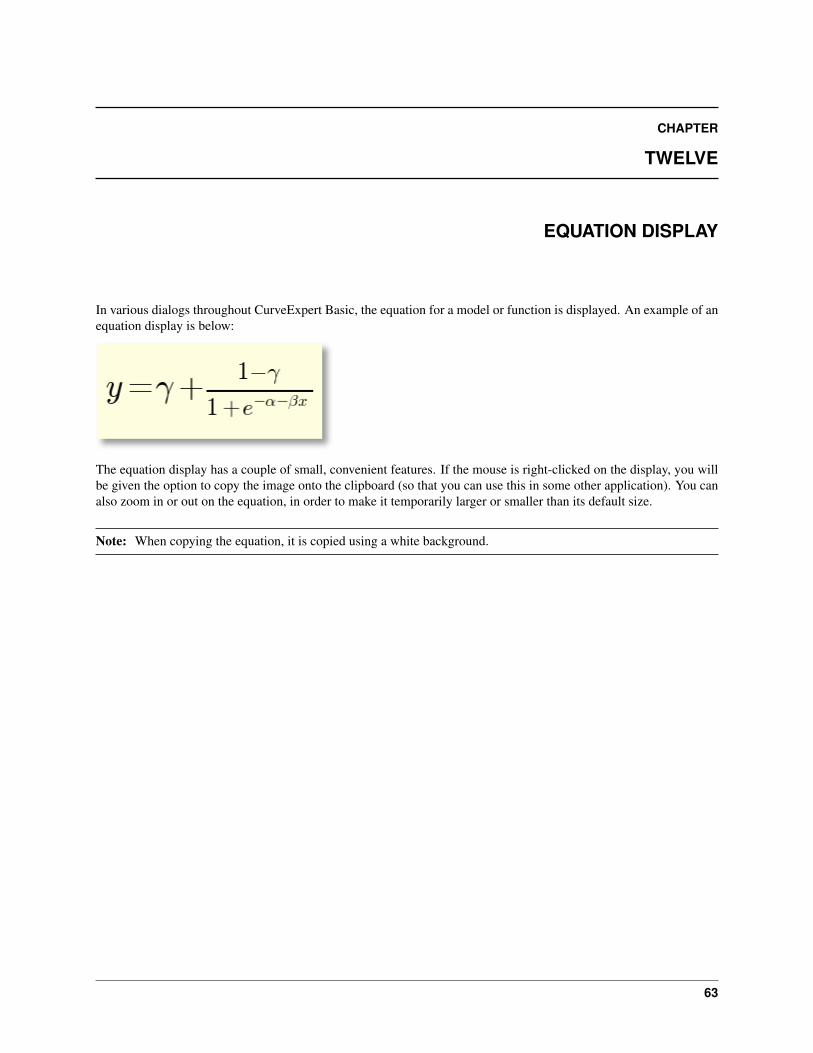
CHAPTER
TWELVE
EQUATION DISPLAY
In various dialogs throughout CurveExpert Basic, the equation for a model or function is displayed. An example of anequation display is below:
The equation display has a couple of small, convenient features. If the mouse is right-clicked on the display, you willbe given the option to copy the image onto the clipboard (so that you can use this in some other application). You canalso zoom in or out on the equation, in order to make it temporarily larger or smaller than its default size.
Note: When copying the equation, it is copied using a white background.
63

CurveExpert Basic Documentation, Release 2.1.0
64 Chapter 12. Equation Display
CHAPTER
THIRTEEN
WRITING DATA
13.1 Introduction
After performing some analysis, a typical task is to write data, in some form, to disk for later retrieval. CurveExpertBasic supports several ways to extract data and graphs to a file or the clipboard.
13.2 Writing a CurveExpert (CXP) file
If you want to save all of your data, results, and graphs to disk, you can choose File->Save or File->Save As in orderto write a CXP file to disk. These files can be read in later using File->Open, obviously. CXP files are portable acrossplatforms (Windows, Mac, Linux) and save all possible information about your current session. CXP files are alsointerchangeable between CurveExpert Professional and CurveExpert Basic.
Also, if a particular model or function is saved as a result in a CXP file and it is not present on the system readingthe file, the model/function will automatically be created (on the system reading the file) on your behalf. This newlycreated model/function will then be available for use in the “Imported” family, and will appear appropriately in theNonlinear model picker.
13.3 Exporting a dataset to text file
To save your dataset into a text file, choose File->Export. The dataset will be exported using the default delimiterchosen in Edit->Preferences->General->Default delimiter.
13.4 Writing a graph to a picture file
To save a particular graph to a file, right click it and select Save. Any graph can be saved wherever it appears via thisprocedure. Alternatively, click the Save icon in the graph toolbar (if present). See Saving graphs for more details onsupported file formats.
The same graph can be copied to the clipboard by right clicking and selecting Copy.
13.5 Printing
All graphs in the Graphs and Data pane can be printed by choosing File->Print or File->Print Preview. To print anindividual graph, right click it and select Print or Print Preview.
65

CurveExpert Basic Documentation, Release 2.1.0
If the margins or paper orientation is not correct, you can set these in the File->Page Setup dialog.
66 Chapter 13. Writing Data
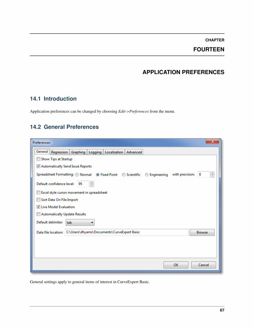
CHAPTER
FOURTEEN
APPLICATION PREFERENCES
14.1 Introduction
Application preferences can be changed by choosing Edit->Preferences from the menu.
14.2 General Preferences
General settings apply to general items of interest in CurveExpert Basic.
67
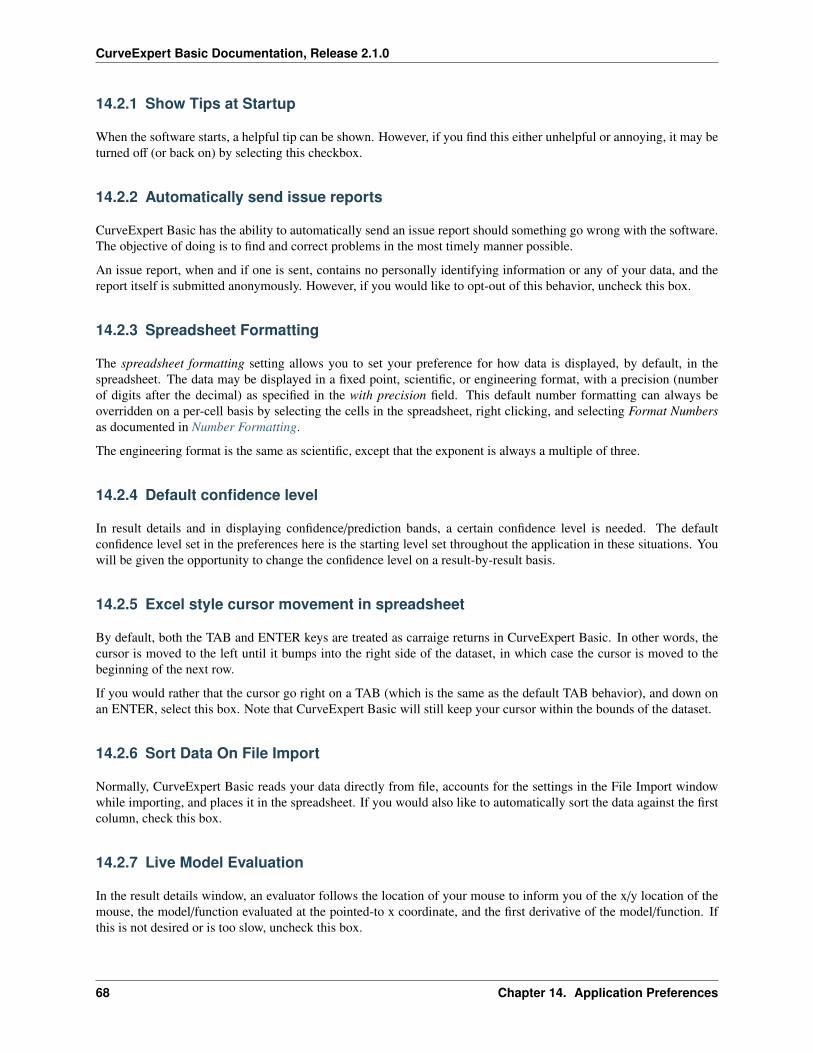
CurveExpert Basic Documentation, Release 2.1.0
14.2.1 Show Tips at Startup
When the software starts, a helpful tip can be shown. However, if you find this either unhelpful or annoying, it may beturned off (or back on) by selecting this checkbox.
14.2.2 Automatically send issue reports
CurveExpert Basic has the ability to automatically send an issue report should something go wrong with the software.The objective of doing is to find and correct problems in the most timely manner possible.
An issue report, when and if one is sent, contains no personally identifying information or any of your data, and thereport itself is submitted anonymously. However, if you would like to opt-out of this behavior, uncheck this box.
14.2.3 Spreadsheet Formatting
The spreadsheet formatting setting allows you to set your preference for how data is displayed, by default, in thespreadsheet. The data may be displayed in a fixed point, scientific, or engineering format, with a precision (numberof digits after the decimal) as specified in the with precision field. This default number formatting can always beoverridden on a per-cell basis by selecting the cells in the spreadsheet, right clicking, and selecting Format Numbersas documented in Number Formatting.
The engineering format is the same as scientific, except that the exponent is always a multiple of three.
14.2.4 Default confidence level
In result details and in displaying confidence/prediction bands, a certain confidence level is needed. The defaultconfidence level set in the preferences here is the starting level set throughout the application in these situations. Youwill be given the opportunity to change the confidence level on a result-by-result basis.
14.2.5 Excel style cursor movement in spreadsheet
By default, both the TAB and ENTER keys are treated as carraige returns in CurveExpert Basic. In other words, thecursor is moved to the left until it bumps into the right side of the dataset, in which case the cursor is moved to thebeginning of the next row.
If you would rather that the cursor go right on a TAB (which is the same as the default TAB behavior), and down onan ENTER, select this box. Note that CurveExpert Basic will still keep your cursor within the bounds of the dataset.
14.2.6 Sort Data On File Import
Normally, CurveExpert Basic reads your data directly from file, accounts for the settings in the File Import windowwhile importing, and places it in the spreadsheet. If you would also like to automatically sort the data against the firstcolumn, check this box.
14.2.7 Live Model Evaluation
In the result details window, an evaluator follows the location of your mouse to inform you of the x/y location of themouse, the model/function evaluated at the pointed-to x coordinate, and the first derivative of the model/function. Ifthis is not desired or is too slow, uncheck this box.
68 Chapter 14. Application Preferences

CurveExpert Basic Documentation, Release 2.1.0
There also an intermediate state for this checkbox; if set to intermediate, the live evaluator will activate when the leftmouse button is pressed only (by default).
14.2.8 Automatically Update Results
If you have already calculated results and then change the data, the results become invalid (see Working with Results).This state is indicated by a yellow caution badge placed on the results in the Results pane. To update these results,you can select some (or all), right click, and select Update. To automatically update results without having to do ityourself, check this box. As soon as a change in the data is detected, all results will be recomputed.
14.2.9 Default delimiter
In several places in the software, a delimiter is used to separate items in the same row. For example, in copying datato the clipoboard, or in generating a table, a delimiter between data items must be selected. If you have a favoritedelimiter, set it here.
14.2.10 Data file location
Default directory where data files are stored. Initially, the data file location is set to $DOCUMENTS/CurveExpertBasic, and some example data and example documents are placed there at install time.
14.2. General Preferences 69
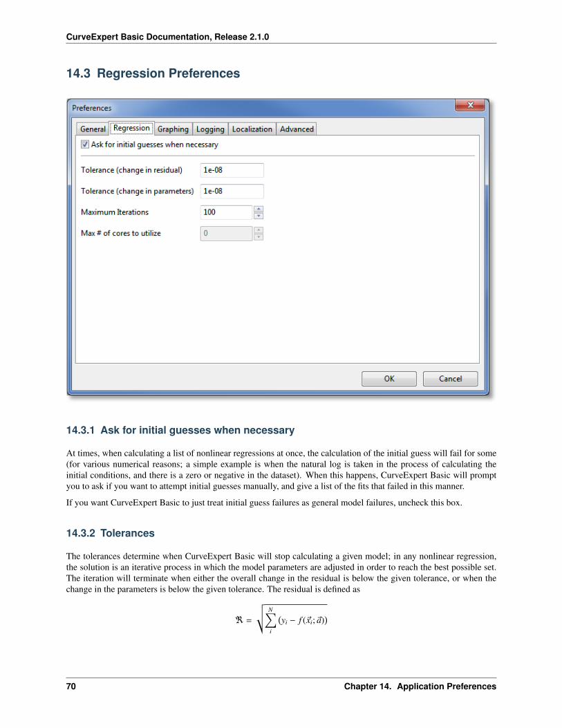
CurveExpert Basic Documentation, Release 2.1.0
14.3 Regression Preferences
14.3.1 Ask for initial guesses when necessary
At times, when calculating a list of nonlinear regressions at once, the calculation of the initial guess will fail for some(for various numerical reasons; a simple example is when the natural log is taken in the process of calculating theinitial conditions, and there is a zero or negative in the dataset). When this happens, CurveExpert Basic will promptyou to ask if you want to attempt initial guesses manually, and give a list of the fits that failed in this manner.
If you want CurveExpert Basic to just treat initial guess failures as general model failures, uncheck this box.
14.3.2 Tolerances
The tolerances determine when CurveExpert Basic will stop calculating a given model; in any nonlinear regression,the solution is an iterative process in which the model parameters are adjusted in order to reach the best possible set.The iteration will terminate when either the overall change in the residual is below the given tolerance, or when thechange in the parameters is below the given tolerance. The residual is defined as
ℜ =
⎯N∑i
(yi − f (~xi;~a)
)
70 Chapter 14. Application Preferences
CurveExpert Basic Documentation, Release 2.1.0
14.3.3 Maximum Iterations
The iteration described in “Tolerances” above can also be terminated when the number of iterations reaches a certainthreshhold. That threshhold is specified in this field.
14.4 Graphing Preferences
14.4.1 Max display points
Sets the maximum number of points, per series, to display when drawing a discrete dataset on a graph. If the datasethas more points than this, it will be thinned to this number of points. The thinning is based on an appropriate stride touse in order to reduce the total number of points drawn to below the threshhold given here. This option is in place toprevent extremely slow graph redraws due to attempting to draw an excessive number of points.
This option affects discrete datasets only; not continuous functions. For continuous functions, the Resolution param-eter, in the Series Page of the Graph Properties dialog (see Changing Graph Properties), is the way to control thesampling of the function that is used for drawing.
14.4.2 Autoscale when model/function added
When a model or function is added to a graph (via a Send to Plot command or a drag and drop), CurveExpert Basiccan automatically autoscale the graph. In this case, you can set the preference to “Never” or “Always”. If the autoscale
14.4. Graphing Preferences 71
CurveExpert Basic Documentation, Release 2.1.0
lock has been set for a graph (see Graph Toolbar), the graph will not be autoscaled regardless of this setting; in otherwords, the graph’s autoscale lock takes precedence over this preference.
14.4.3 Autoscale when data changed
In order to keep the data in view at all times in all graphs, CurveExpert Basic can automatically autoscale the graphswhen the underlying dataset changes. The disadvantage of doing this is that, for large datasets, the redraw can beslow. Also, if you have specified your own limits to axes in the graphs, they would be lost if the data changes. If theautoscale lock has been set for a graph (see Graph Toolbar), the graph will not be autoscaled regardless of this setting;in other words, the graph’s autoscale lock takes precedence over this preference.
To control when autoscaling takes place, select either “Never” or “Always”.
14.4.4 Autoscale when model/function removed
When a model or function is removed from a graph (either by removing the result from your document altogether, orby right clicking a result on a plot and selecting “Remove”), CurveExpert Basic can automatically autoscale the graph.In this case, you can set the preference to “Never” or “Always”. If the autoscale lock has been set for a graph (seeGraph Toolbar), the graph will not be autoscaled regardless of this setting; in other words, the graph’s autoscale locktakes precedence over this preference.
14.4.5 Highlight pickable objects
As you move the mouse over a curve or data, it will highlight, signifying that you can click it to modify its properties.Also, it signifies that, on right-click, you can access the details for that series. However, the redrawing necessary forthis feature can make the graph response sluggish. So, deactivate this feature if you don’t need to see the highlightingor access details directly from the graph.
14.4.6 Continuous redraw during pan
During a pan, all continuous series must be regenerated on-the-fly if this feature is turned on. This can be expensive,so if it is OK not to see the curve dynamically update during a pan, turn this checkbox off. The series will then onlybe regenerated each time the mouse button is released during a panning operation.
As a reminder, this setting does not affect discrete datasets on the graph; only results that are continuous.
14.4.7 Automatically plot top # results
When computing batches of nonlinear regressions at once, if all of them were plotted on the “Top Results” graph, itwould be quite messy. Here, you can decide how many of the results will be plotted on the graph for each batch thatyou compute. The default behavior is to take the best three fits for every batch that you compute. Other results that youwant to visualize can always be added by right clicking them and selecting Send to Plot, or by dragging and droppingthe result to the plot.
14.4.8 Preserve aspect ratio when printing
Normally, any graph is fit to the page when it is printed. If you would like to preserve the aspect ratio of your graphwhen printing, check this box. In other words, if you have a graph that is long and skinny, to keep it long and skinnywhen printed, check this box.
72 Chapter 14. Application Preferences
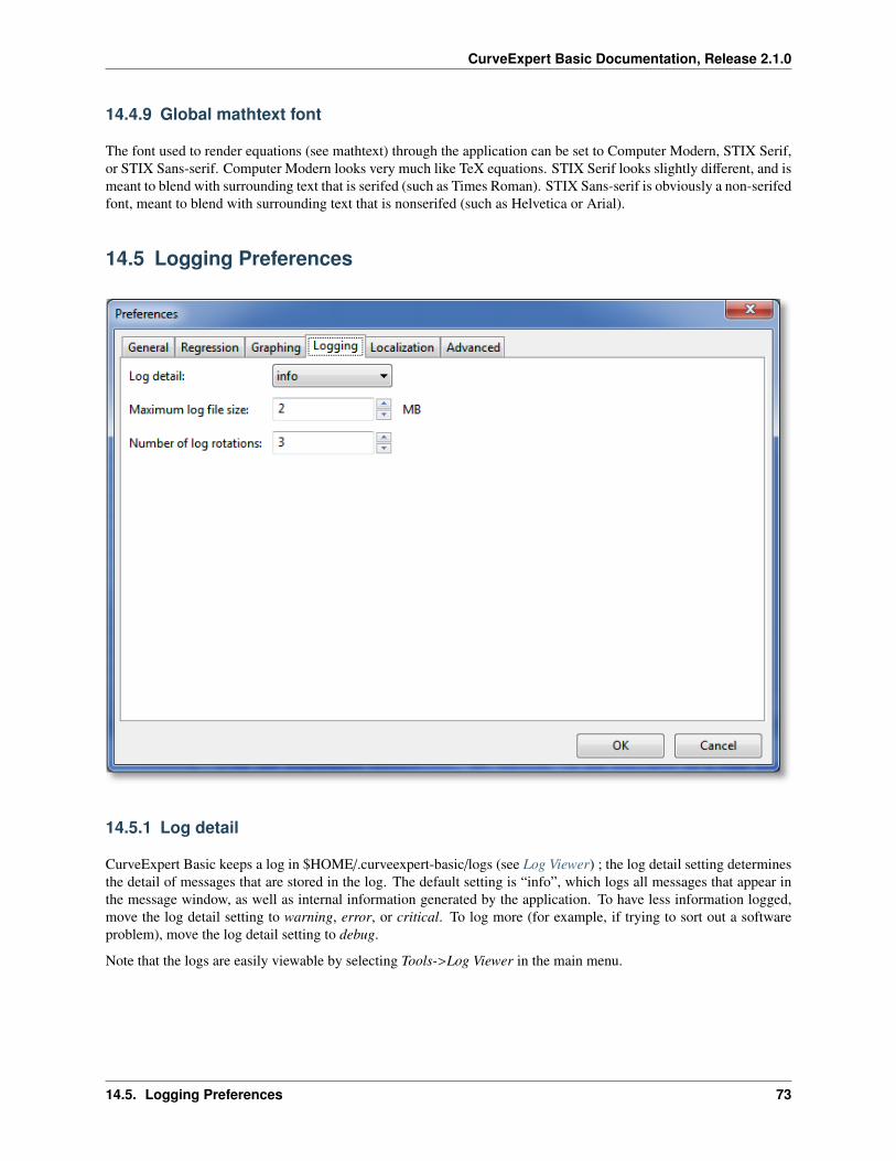
CurveExpert Basic Documentation, Release 2.1.0
14.4.9 Global mathtext font
The font used to render equations (see mathtext) through the application can be set to Computer Modern, STIX Serif,or STIX Sans-serif. Computer Modern looks very much like TeX equations. STIX Serif looks slightly different, and ismeant to blend with surrounding text that is serifed (such as Times Roman). STIX Sans-serif is obviously a non-serifedfont, meant to blend with surrounding text that is nonserifed (such as Helvetica or Arial).
14.5 Logging Preferences
14.5.1 Log detail
CurveExpert Basic keeps a log in $HOME/.curveexpert-basic/logs (see Log Viewer) ; the log detail setting determinesthe detail of messages that are stored in the log. The default setting is “info”, which logs all messages that appear inthe message window, as well as internal information generated by the application. To have less information logged,move the log detail setting to warning, error, or critical. To log more (for example, if trying to sort out a softwareproblem), move the log detail setting to debug.
Note that the logs are easily viewable by selecting Tools->Log Viewer in the main menu.
14.5. Logging Preferences 73
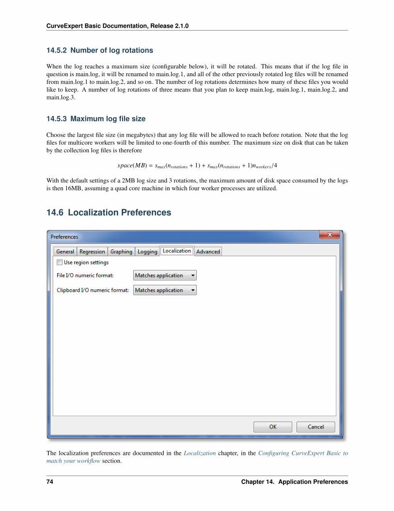
CurveExpert Basic Documentation, Release 2.1.0
14.5.2 Number of log rotations
When the log reaches a maximum size (configurable below), it will be rotated. This means that if the log file inquestion is main.log, it will be renamed to main.log.1, and all of the other previously rotated log files will be renamedfrom main.log.1 to main.log.2, and so on. The number of log rotations determines how many of these files you wouldlike to keep. A number of log rotations of three means that you plan to keep main.log, main.log.1, main.log.2, andmain.log.3.
14.5.3 Maximum log file size
Choose the largest file size (in megabytes) that any log file will be allowed to reach before rotation. Note that the logfiles for multicore workers will be limited to one-fourth of this number. The maximum size on disk that can be takenby the collection log files is therefore
space(MB) = smax(nrotations + 1) + smax(nrotations + 1)nworkers/4
With the default settings of a 2MB log size and 3 rotations, the maximum amount of disk space consumed by the logsis then 16MB, assuming a quad core machine in which four worker processes are utilized.
14.6 Localization Preferences
The localization preferences are documented in the Localization chapter, in the Configuring CurveExpert Basic tomatch your workflow section.
74 Chapter 14. Application Preferences
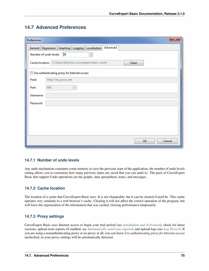
CurveExpert Basic Documentation, Release 2.1.0
14.7 Advanced Preferences
14.7.1 Number of undo levels
Any undo mechanism consumes some memory to save the previous state of the application; the number of undo levelssetting allows you to customize how many previous states are saved that you can undo to. The parts of CurveExpertBasic that support Undo operations are the graphs, data spreadsheet, notes, and messages.
14.7.2 Cache location
The location of a cache that CurveExpert Basic uses. It is not changeable, but it can be cleared if need be. This cacheoperates very similarly to a web browser’s cache. Clearing it will not affect the correct operation of the program, butwill force the regeneration of the information that was cached, slowing performance temporarily.
14.7.3 Proxy settings
CurveExpert Basic uses Internet access to begin your trial period (see Installation and Activation), check for latestversions, upload issue reports (if enabled, see Automatically send issue reports), and upload logs (see Log Viewer). Ifyou are using a nonauthenticating proxy or no proxy at all, you can leave Use authenticating proxy for Internet accessunchecked, as your proxy settings will be automatically detected.
14.7. Advanced Preferences 75

CurveExpert Basic Documentation, Release 2.1.0
However, if you are behind a proxy that requires authentication, please fill in the host, port, username, and passwordfor access through the proxy.
76 Chapter 14. Application Preferences

CHAPTER
FIFTEEN
LOCALIZATION
15.1 Executive Summary
If you live in a locale that uses dots for decimals (such as the US or UK) and you never (or very rarely) read files thatuse European-style commas-for-decimals, the issues in this chapter are of no interest to you.
If you live in a locale that uses commas for decimals, and you want to see commas throughout the application,select Use region settings in the application preferences. Further, if you need to read files that use the dot-decimalnotation most often, select “English” for File I/O numeric format.
If you live in a locale that uses commas for decimals, and you do not want to see commas throughout theapplication, unselect Use region settings in the application preferences. Further, if you need to read files that use thecomma-decimal notation most often, select “European” for “File I/O numeric format”. Also, if you want to be able tocut/paste to/from Excel, which obeys locale settings, select “European” for Clipboard I/O numeric format.
15.2 Configuring CurveExpert Basic to match your workflow
15.2.1 Use region settings
The main “switch” is in Edit->Preferences->Localization->Use region settings. If this is checked, CurveExpert Basicuses the region settings as given by the operating system. Any display of a number uses your localized representation,which means that if you live in a locale that uses commas for decimals, all numbers that appear in the spreadsheet,results, etc. use commas. Copying to clipboard uses commas, pasting from clipboard expects commas, writing to files(file export, tables) uses commas, the reading from files expects commas. In other words, the application respects thelocale completely.
If Use region settings is left unchecked, the “C” locale is used, which always uses dots for decimals. You are still freeto modify the File I/O and Clipboard I/O settings below to match your workflow.
15.2.2 File I/O numeric format
The Edit->Preferences->Localization->File I/O numeric format choice allows you to override the application-widelocale setting for file input/output, to explicitly define the numeric format for reading and writing files. This affects thefile import dialog as well as File->Export, and the table generator in the result details window. With this setting, forexample, users that utilize commas for decimals in CurveExpert Basic can choose to read and write files using dotsfor decimals. And vice versa.
77
CurveExpert Basic Documentation, Release 2.1.0
Note: In the file import dialog (see Raw file import), there is still a chance to change the numeric format beforereading the file. This setting simply sets the default numeric format in that dialog appropriately.
15.2.3 Clipboard I/O numeric format
The Edit->Preferences->Localization->Clipboard I/O numeric format choice allows you to override the application-wide locale setting for clipboard input/output, to explicitly define the numeric format for copying and pasting. Thisaffects the copy/paste in the spreadsheet, as well as copying numeric data out any window that might offer it. With thissetting, for example, users that utilize commas for decimals in CurveExpert Basic can choose to copy and paste datato/from the clipboard using dots for decimals. And vice versa.
15.2.4 File Import: numeric format
In the file import dialog (File->Open), there is a switch to explicitly pick the numerical formatting (English or Euro-pean style) before reading the file. This gives the user the opportunity, on a file-by-file basis, to specify the numericalformat. See Raw file import.
15.3 File overrides
If your file contains the following within the first ten lines of the file:
#DataFileProperties: locale=EN
or:
#DataFileProperties: locale=EURO
this signals to the CurveExpert Basic file importing mechanism that the the file uses English or European numericalformatting (as appropriate), and the default there (see Raw file import) will be set appropriately. The user may stilloverride the default, however, but in most cases this would be a bad idea, because the file itself is stating what thecorrect locale is.
So, you can use this capability in your own data files if you like. All of the sample data files shipped with CurveEx-pert Basic contain this line, so that the samples work straightforwardly regardless of the application’s current regionsettings. This small addition to a text datafile lets the file itself express its own numerical formatting.
15.4 CurveExpert Basic files
CurveExpert Basic files (.cxp) are not affected by region settings; therefore, they are portable across localities as wellas being portable across platforms (Windows, Mac, Linux).
15.5 NIST verification files
The data files associated with the NIST datasets are explicitly US-locale, and are treated as such when they are readin as a result of Tools->Run NIST Validation performed within CurveExpert Basic (see Validation). However, if you
78 Chapter 15. Localization

CurveExpert Basic Documentation, Release 2.1.0
read these files in yourself, note that you MUST select an English numerical formatting in the file import dialog, if itis not already set.
15.5. NIST verification files 79

CurveExpert Basic Documentation, Release 2.1.0
80 Chapter 15. Localization
CHAPTER
SIXTEEN
VALIDATION
16.1 Introduction
CurveExpert Basic is validated against the Statistical Reference Datasets Project of the National Institute of Standardsand Technology. These datasets can be downloaded directly at http://www.itl.nist.gov/div898/strd/general/dataarchive.html, but are also included verbatim in the CurveExpert Basic distribution for you to use yourself. The datasetsvalidated against are all of the sets in the “Linear Regression” and “Nonlinear Regression” categories.
16.2 Running the Suite
You can validate CurveExpert Basic against these datasets simply by choosing Tools->Run NIST Validation. Allvalidation cases, with all “starts”, will be run. The NIST test suite provides different starts (i.e., initial guesses) foreach nonlinear regression validation. CurveExpert Basic covers all of these starts in the test suite, and the results areoutput to the message window.
Some competing packages do not include all starts in their validation sets, but CurveExpert Basic shows the results ofall of them. At the time of this writing, there is one failure (dataset BoxBOD, Start #1), where, for the given start, theinitial correction to parameter β2 causes underflow in the model, and from this there is no recovery.
16.3 Performing validations yourself
If you would like to perform validations against the test data yourself, all data files are contained in the “exam-ple_data/NIST” folder in the initial data directory (see Where files are located). Or, you can always download the filesfrom NIST at the link above.
Note: The NIST datasets all list the dependent variable (usually y) before the independent variable (usually x). So,when you read the files, select Rotate Columns in the file import dialog, or alternatively, rotate the columns after youread in the dataset.
All nonlinear regression validation runs are performed in the automated suite with rtol=ptol=1.0e-14, and max-iter=1000.
81

CurveExpert Basic Documentation, Release 2.1.0
82 Chapter 16. Validation
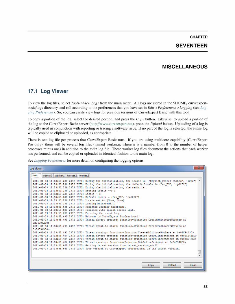
CHAPTER
SEVENTEEN
MISCELLANEOUS
17.1 Log Viewer
To view the log files, select Tools->View Logs from the main menu. All logs are stored in the $HOME/.curveexpert-basic/logs directory, and roll according to the preferences that you have set in Edit->Preferences->Logging (see Log-ging Preferences). So, you can easily view logs for previous sessions of CurveExpert Basic with this tool.
To copy a portion of the log, select the desired portion, and press the Copy button. Likewise, to upload a portion ofthe log to the CurveExpert Basic server (http://www.curveexpert.net), press the Upload button. Uploading of a log istypically used in conjunction with reporting or tracing a software issue. If no part of the log is selected, the entire logwill be copied to clipboard or uploaded, as appropriate.
There is one log file per process that CurveExpert Basic runs. If you are using multicore capability (CurveExpertPro only), there will be several log files (named worker.n, where n is a number from 0 to the number of helperprocesses minus one) in addition to the main log file. These worker log files document the actions that each workerhas performed, and can be copied or uploaded in identical fashion to the main log.
See Logging Preferences for more detail on configuring the logging options.
83
CurveExpert Basic Documentation, Release 2.1.0
17.2 Running Multiple Instances
Running multiple instances of CurveExpert Basic is supported; the only side effect is that, because all instances sharethe same log files, logging might not function properly.
17.3 Where files are located
CurveExpert Basic places files in several locations on disk; the locations are documented below.
17.3.1 Program Files
The default locations are listed below, assuming that the default is accepted during the installation process. If you havechanged the location of the program files, obviously they will be placed where you specified.
Platform Program Files LocationWindows (64 bit) c:\Program Files (x86)\CurveExpert BasicWindows (32 bit) c:\Program Files\CurveExpert Basic
17.3.2 Application Settings
Platform Application Settings LocationWindows in registry: HKEY_CURRENT_USER\Software\CurveExpert Basic
17.3.3 Working/Cache Area
An area is reserved for various caches and items that are needed for normal application operation. This area is usedfor the cache, logs, and storage of custom user models.
Platform Working/Cache Area LocationWindows $HOME\.curveexpert-basic
17.3.4 CurveExpert Basic Data Files
The data files directory can be customized using Edit->Preferences->General, but the default locations are below.This directory is also where the example data that ships with CurveExpert resides.
Platform Documents LocationWindows $MYDOCUMENTS\CurveExpert Basic
84 Chapter 17. Miscellaneous
CHAPTER
EIGHTEEN
END USER LICENSE AGREEMENT
IMPORTANT – READ CAREFULLY: This End-User License Agreement (“EULA”) is a legal agreement betweenyou (either an individual or single entity) and Mr. Daniel Hyams of 115 Cresthaven Drive, Madison, AL 35758(“Mr.Hyams”) for the software product “CurveExpert Basic”, which will be designated by the term “Software Product”. TheSoftware Product consists computer software and accompanying electronic documentation. By installing, copying, orotherwise using the Software Product, you agree to be bound by the terms of this EULA. If you do not agree to theterms of this EULA, do not install or use the Software Product.
1. Grant of License. Mr. Hyams grants to you as an individual, a personal, nonexclusive license to make and usecopies of the Software Product. Copies must be made only for backup or archival purposes.
2. Shareware version. You are hereby granted a non-exclusive license to use the Software Product for an evalu-ation period of 30 days, after which you must pay the registration fee to continue using the Software Product.However, use of the Software Product during the 30-day evaluation period is free of charge. Unregistered use ofthe Software Product after the 30-day evaluation period is in violation of Federal copyright laws and the termsof this EULA. Violators will be prosecuted to the maximum extent under the law. You may make exact copiesand distribute the shareware version of the Software Product and its documentation so long as there is no chargeapplied to distribution of these unmodified copies of the Software Product. You are specifically prohibited fromcharging or requesting donations for ANY and ALL copies of this Software Product or its documentation. Youare prohibited from distributing the Software Product or any portion of the Software Product or its documenta-tion as part of another product (commercial or otherwise) without PRIOR expressed written consent from Mr.Hyams.
3. Registered Version If you have registered the Software Product with Mr. Hyams (meaning to remit payment forpurchase of the software), the 30-day evaluation period in Section 2 is waived. Mr. Hyams agrees to provide youwith valid license key for the Software Product, copied onto media deemed suitable, within 30 days of receiptof payment.
4. Reverse engineering. You may not reverse engineer, decompile, or disassemble the Software Product.
5. Upgrades. All subsequent versions of the software product fall under the terms of this EULA. Upgrades aredesignated as software packages of the same name but with an incremented version number.
6. Copyright. All title and copyrights in and to the Software Product are owned by Mr. Hyams. The SoftwareProduct is protected by copyright laws and international treaty provisions.
7. Warranty Disclaimer. The Software Product and the accompanying files are sold “as is” without warrantyof any kind. All warranties, either express or implied, including, but not limited to, implied warranties ofmerchantability and fitness for a particular purpose, are expressly and specifically disclaimed.
8. Liability. Neither Mr. Hyams or anyone else who has been involved in the creation, production, or deliveryof this Software Product shall be liable for any direct, indirect, consequential, special, incidental, or similardamages arising out of the use or inability to use such software even if Mr. Hyams has been advised of thepossibility of such damages or claims. In no event shall Mr. Hyams’s liability for any damages ever exceed theprice paid for the license to the Software Product, regardless of the form of the claim. The individual using theSoftware Product bears all risk as to the quality and performance of the Software Product.
85

CurveExpert Basic Documentation, Release 2.1.0
9. Governing Law. This agreement shall be governed by the laws of the State of Alabama and shall inure to thebenefit of Mr. Hyams, his heirs, successors, and assigns. Any action or proceeding brought by either partyagainst the other arising out of or relating to this agreement shall be brought only in a state or federal court ofcompetent jurisdiction located in Madison, Alabama. The parties hereby consent to in personam jurisdiction ofsaid courts.
86 Chapter 18. End User License Agreement

CHAPTER
NINETEEN
THIRD-PARTY LICENSING
CurveExpert Basic owes its existence to several excellent open source packages. This section is in the documentationin order to comply with licensing requirements of these packages.
19.1 Python
PSF LICENSE AGREEMENT FOR PYTHON 2.6.6
1. This LICENSE AGREEMENT is between the Python Software Foundation (“PSF”), and the Individual orOrganization (“Licensee”) accessing and otherwise using Python 2.6.6 software in source or binary form and itsassociated documentation.
2. Subject to the terms and conditions of this License Agreement, PSF hereby grants Licensee a nonexclusive,royalty-free, world-wide license to reproduce, analyze, test, perform and/or display publicly, prepare deriva-tive works, distribute, and otherwise use Python 2.6.6 alone or in any derivative version, provided, however,that PSF’s License Agreement and PSF’s notice of copyright, i.e., “Copyright © 2001-2010 Python SoftwareFoundation; All Rights Reserved” are retained in Python 2.6.6 alone or in any derivative version prepared byLicensee.
3. In the event Licensee prepares a derivative work that is based on or incorporates Python 2.6.6 or any part thereof,and wants to make the derivative work available to others as provided herein, then Licensee hereby agrees toinclude in any such work a brief summary of the changes made to Python 2.6.6.
4. PSF is making Python 2.6.6 available to Licensee on an “AS IS” basis. PSF MAKES NO REPRESENTA-TIONS OR WARRANTIES, EXPRESS OR IMPLIED. BY WAY OF EXAMPLE, BUT NOT LIMITATION,PSF MAKES NO AND DISCLAIMS ANY REPRESENTATION OR WARRANTY OF MERCHANTABIL-ITY OR FITNESS FOR ANY PARTICULAR PURPOSE OR THAT THE USE OF PYTHON 2.6.6 WILL NOTINFRINGE ANY THIRD PARTY RIGHTS.
5. PSF SHALL NOT BE LIABLE TO LICENSEE OR ANY OTHER USERS OF PYTHON 2.6.6 FOR ANYINCIDENTAL, SPECIAL, OR CONSEQUENTIAL DAMAGES OR LOSS AS A RESULT OF MODIFYING,DISTRIBUTING, OR OTHERWISE USING PYTHON 2.6.6, OR ANY DERIVATIVE THEREOF, EVEN IFADVISED OF THE POSSIBILITY THEREOF.
6. This License Agreement will automatically terminate upon a material breach of its terms and conditions.
7. Nothing in this License Agreement shall be deemed to create any relationship of agency, partnership, or jointventure between PSF and Licensee. This License Agreement does not grant permission to use PSF trademarksor trade name in a trademark sense to endorse or promote products or services of Licensee, or any third party.
8. By copying, installing or otherwise using Python 2.6.6, Licensee agrees to be bound by the terms and conditionsof this License Agreement.
87

CurveExpert Basic Documentation, Release 2.1.0
19.2 WxWidgets and WxPython
19.2.1 Preamble
The licensing of the wxWidgets library is intended to protect the wxWidgets library, its developers, and its users, sothat the considerable investment it represents is not abused.
Under the terms of the wxWindows licence, you as a user are not obliged to distribute wxWidgets source code withyour products, if you distribute these products in binary form. However, you are prevented from restricting use of thelibrary in source code form, or denying others the rights to use or distribute wxWidgets library source code in the wayintended.
The wxWindows licence establishes the copyright for the code and related material, and it gives you legal permissionto copy, distribute and/or modify the library. It also asserts that no warranty is given by the authors for this or derivedcode.
The core distribution of the wxWidgets library contains files under two different licences:
• Most files are distributed under the GNU Library General Public Licence, version 2, with the special exceptionthat you may create and distribute object code versions built from the source code or modified versions of it(even if these modified versions include code under a different licence), and distribute such binaries under yourown terms.
• Most core wxWidgets manuals are made available under the “wxWidgets Free Documentation Licence”, whichallows you to distribute modified versions of the manuals, such as versions documenting any modifications madeby you in your version of the library. However, you may not restrict any third party from reincorporating yourchanges into the original manuals.
Other relevant files:
• licence.txt: a statement that the wxWidgets library is covered by the GNU Library General Public Licence, withan exception notice for binary distribution.
• licendoc.txt: the wxWidgets Documentation Licence.
• lgpl.txt: the text of the GNU Library General Public Licence.
• gpl.txt: the text of the GNU General Public Licence, which is referenced by the LGPL.
19.2.2 wxWindows Library License, Version 3.1
Copyright (c) 1998-2005 Julian Smart, Robert Roebling et al
Everyone is permitted to copy and distribute verbatim copies of this licence document, but changing it isnot allowed.
WXWINDOWS LIBRARY LICENCE
TERMS AND CONDITIONS FOR COPYING, DISTRIBUTION AND MODIFICATION
This library is free software; you can redistribute it and/or modify it under the terms of the GNU LibraryGeneral Public Licence as published by the Free Software Foundation; either version 2 of the Licence, or(at your option) any later version.
This library is distributed in the hope that it will be useful, but WITHOUT ANY WARRANTY; withouteven the implied warranty of MERCHANTABILITY or FITNESS FOR A PARTICULAR PURPOSE.See the GNU Library General Public Licence for more details.
88 Chapter 19. Third-Party Licensing

CurveExpert Basic Documentation, Release 2.1.0
You should have received a copy of the GNU Library General Public Licence along with this software,usually in a file named COPYING.LIB. If not, write to the Free Software Foundation, Inc., 59 TemplePlace, Suite 330, Boston, MA 02111-1307 USA.
EXCEPTION NOTICE
1. As a special exception, the copyright holders of this library give permission for additional uses of thetext contained in this release of the library as licenced under the wxWindows Library Licence, applyingeither version 3.1 of the Licence, or (at your option) any later version of the Licence as published by thecopyright holders of version 3.1 of the Licence document.
2. The exception is that you may use, copy, link, modify and distribute under your own terms, binaryobject code versions of works based on the Library.
3. If you copy code from files distributed under the terms of the GNU General Public Licence or the GNULibrary General Public Licence into a copy of this library, as this licence permits, the exception does notapply to the code that you add in this way. To avoid misleading anyone as to the status of such modifiedfiles, you must delete this exception notice from such code and/or adjust the licensing conditions noticeaccordingly.
4. If you write modifications of your own for this library, it is your choice whether to permit this exceptionto apply to your modifications. If you do not wish that, you must delete the exception notice from suchcode and/or adjust the licensing conditions notice accordingly.
19.3 Numpy
Copyright (c) 2005-2009, NumPy Developers. All rights reserved.
Redistribution and use in source and binary forms, with or without modification, are permitted provided that thefollowing conditions are met:
• Redistributions of source code must retain the above copyright notice, this list of conditions and the followingdisclaimer.
• Redistributions in binary form must reproduce the above copyright notice, this list of conditions and the follow-ing disclaimer in the documentation and/or other materials provided with the distribution.
• Neither the name of the NumPy Developers nor the names of any contributors may be used to endorse or promoteproducts derived from this software without specific prior written permission.
THIS SOFTWARE IS PROVIDED BY THE COPYRIGHT HOLDERS AND CONTRIBUTORS “AS IS” AND ANYEXPRESS OR IMPLIED WARRANTIES, INCLUDING, BUT NOT LIMITED TO, THE IMPLIED WARRANTIESOF MERCHANTABILITY AND FITNESS FOR A PARTICULAR PURPOSE ARE DISCLAIMED. IN NO EVENTSHALL THE COPYRIGHT OWNER OR CONTRIBUTORS BE LIABLE FOR ANY DIRECT, INDIRECT, IN-CIDENTAL, SPECIAL, EXEMPLARY, OR CONSEQUENTIAL DAMAGES (INCLUDING, BUT NOT LIMITEDTO, PROCUREMENT OF SUBSTITUTE GOODS OR SERVICES; LOSS OF USE, DATA, OR PROFITS; OR BUSI-NESS INTERRUPTION) HOWEVER CAUSED AND ON ANY THEORY OF LIABILITY, WHETHER IN CON-TRACT, STRICT LIABILITY, OR TORT (INCLUDING NEGLIGENCE OR OTHERWISE) ARISING IN ANYWAY OUT OF THE USE OF THIS SOFTWARE, EVEN IF ADVISED OF THE POSSIBILITY OF SUCH DAM-AGE.
19.4 Scipy
Copyright (c) 2001, 2002 Enthought, Inc. All rights reserved.
Copyright (c) 2003-2009 SciPy Developers. All rights reserved.
19.3. Numpy 89
CurveExpert Basic Documentation, Release 2.1.0
Redistribution and use in source and binary forms, with or without modification, are permitted provided that thefollowing conditions are met:
1. Redistributions of source code must retain the above copyright notice, this list of conditions and the followingdisclaimer.
2. Redistributions in binary form must reproduce the above copyright notice, this list of conditions and the follow-ing disclaimer in the documentation and/or other materials provided with the distribution.
3. Neither the name of the Enthought nor the names of its contributors may be used to endorse or promote productsderived from this software without specific prior written permission.
THIS SOFTWARE IS PROVIDED BY THE COPYRIGHT HOLDERS AND CONTRIBUTORS “AS IS” AND ANYEXPRESS OR IMPLIED WARRANTIES, INCLUDING, BUT NOT LIMITED TO, THE IMPLIED WARRANTIESOF MERCHANTABILITY AND FITNESS FOR A PARTICULAR PURPOSE ARE DISCLAIMED. IN NO EVENTSHALL THE REGENTS OR CONTRIBUTORS BE LIABLE FOR ANY DIRECT, INDIRECT, INCIDENTAL, SPE-CIAL, EXEMPLARY, OR CONSEQUENTIAL DAMAGES (INCLUDING, BUT NOT LIMITED TO, PROCURE-MENT OF SUBSTITUTE GOODS OR SERVICES; LOSS OF USE, DATA, OR PROFITS; OR BUSINESS INTER-RUPTION) HOWEVER CAUSED AND ON ANY THEORY OF LIABILITY, WHETHER IN CONTRACT, STRICTLIABILITY, OR TORT (INCLUDING NEGLIGENCE OR OTHERWISE) ARISING IN ANY WAY OUT OF THEUSE OF THIS SOFTWARE, EVEN IF ADVISED OF THE POSSIBILITY OF SUCH DAMAGE.
19.5 Matplotlib
Copyright (c) 2002-2007 John D. Hunter; All Rights Reserved
LICENSE AGREEMENT FOR MATPLOTLIB 0.91
1. This LICENSE AGREEMENT is between John D. Hunter (“JDH”), and the Individual or Organization (“Licensee”)accessing and otherwise using matplotlib software in source or binary form and its associated documentation.
2. Subject to the terms and conditions of this License Agreement, JDH hereby grants Licensee a nonexclusive, royalty-free, world-wide license to reproduce, analyze, test, perform and/or display publicly, prepare derivative works, dis-tribute, and otherwise use matplotlib 0.91 alone or in any derivative version, provided, however, that JDH’s LicenseAgreement and JDH’s notice of copyright, i.e., “Copyright (c) 2002-2007 John D. Hunter; All Rights Reserved” areretained in matplotlib 0.91 alone or in any derivative version prepared by Licensee.
3. In the event Licensee prepares a derivative work that is based on or incorporates matplotlib 0.91 or any part thereof,and wants to make the derivative work available to others as provided herein, then Licensee hereby agrees to includein any such work a brief summary of the changes made to matplotlib 0.91.
4. JDH is making matplotlib 0.91 available to Licensee on an “AS IS” basis. JDH MAKES NO REPRESENTATIONSOR WARRANTIES, EXPRESS OR IMPLIED. BY WAY OF EXAMPLE, BUT NOT LIMITATION, JDH MAKESNO AND DISCLAIMS ANY REPRESENTATION OR WARRANTY OF MERCHANTABILITY OR FITNESS FORANY PARTICULAR PURPOSE OR THAT THE USE OF MATPLOTLIB 0.91 WILL NOT INFRINGE ANY THIRDPARTY RIGHTS.
5. JDH SHALL NOT BE LIABLE TO LICENSEE OR ANY OTHER USERS OF MATPLOTLIB 0.91 FOR ANYINCIDENTAL, SPECIAL, OR CONSEQUENTIAL DAMAGES OR LOSS AS A RESULT OF MODIFYING, DIS-TRIBUTING, OR OTHERWISE USING MATPLOTLIB 0.91, OR ANY DERIVATIVE THEREOF, EVEN IF AD-VISED OF THE POSSIBILITY THEREOF.
6. This License Agreement will automatically terminate upon a material breach of its terms and conditions.
7. Nothing in this License Agreement shall be deemed to create any relationship of agency, partnership, or jointventure between JDH and Licensee. This License Agreement does not grant permission to use JDH trademarks ortrade name in a trademark sense to endorse or promote products or services of Licensee, or any third party.
90 Chapter 19. Third-Party Licensing

CurveExpert Basic Documentation, Release 2.1.0
8. By copying, installing or otherwise using matplotlib 0.91, Licensee agrees to be bound by the terms and conditionsof this License Agreement.
19.6 xlrd
CurveExpert Basic utilizes Excel reading capabilities from the xlrd library. This product includes software developedby Roman V. Kiseliov <[email protected]>.
Portions copyright (C) 2007, Stephen John Machin, Lingfo Pty Ltd All rights reserved.
Redistribution and use in source and binary forms, with or without modification, are permitted provided that thefollowing conditions are met:
1. Redistributions of source code must retain the above copyright notice, this list of conditions and the followingdisclaimer.
2. Redistributions in binary form must reproduce the above copyright notice, this list of conditions and the followingdisclaimer in the documentation and/or other materials provided with the distribution.
3. None of the names of Stephen John Machin, Lingfo Pty Ltd and any contributors may be used to endorse or promoteproducts derived from this software without specific prior written permission.
THIS SOFTWARE IS PROVIDED BY THE COPYRIGHT HOLDERS AND CONTRIBUTORS “AS IS” AND ANYEXPRESS OR IMPLIED WARRANTIES, INCLUDING, BUT NOT LIMITED TO, THE IMPLIED WARRANTIESOF MERCHANTABILITY AND FITNESS FOR A PARTICULAR PURPOSE ARE DISCLAIMED. IN NO EVENTSHALL THE COPYRIGHT OWNER OR CONTRIBUTORS BE LIABLE FOR ANY DIRECT, INDIRECT, IN-CIDENTAL, SPECIAL, EXEMPLARY, OR CONSEQUENTIAL DAMAGES (INCLUDING, BUT NOT LIMITEDTO, PROCUREMENT OF SUBSTITUTE GOODS OR SERVICES; LOSS OF USE, DATA, OR PROFITS; OR BUSI-NESS INTERRUPTION) HOWEVER CAUSED AND ON ANY THEORY OF LIABILITY, WHETHER IN CON-TRACT, STRICT LIABILITY, OR TORT (INCLUDING NEGLIGENCE OR OTHERWISE) ARISING IN ANYWAY OUT OF THE USE OF THIS SOFTWARE, EVEN IF ADVISED OF THE POSSIBILITY OF SUCH DAM-AGE.
Copyright (C) 2005 Roman V. Kiseliov All rights reserved.
Redistribution and use in source and binary forms, with or without modification, are permitted provided that thefollowing conditions are met:
1. Redistributions of source code must retain the above copyright notice, this list of conditions and the followingdisclaimer.
2. Redistributions in binary form must reproduce the above copyright notice, this list of conditions and the follow-ing disclaimer in the documentation and/or other materials provided with the distribution.
3. All advertising materials mentioning features or use of this software must display the following acknowledg-ment: This product includes software developed by Roman V. Kiseliov <[email protected]>.
4. Redistributions of any form whatsoever must retain the following acknowledgment: This product includes soft-ware developed by Roman V. Kiseliov <[email protected]>.
THIS SOFTWARE IS PROVIDED BY Roman V. Kiseliov ‘‘AS IS” AND ANY EXPRESSED OR IMPLIED WAR-RANTIES, INCLUDING, BUT NOT LIMITED TO, THE IMPLIED WARRANTIES OF MERCHANTABILITYAND FITNESS FOR A PARTICULAR PURPOSE ARE DISCLAIMED. IN NO EVENT SHALL Roman V. KiseliovOR ITS CONTRIBUTORS BE LIABLE FOR ANY DIRECT, INDIRECT, INCIDENTAL, SPECIAL, EXEMPLARY,OR CONSEQUENTIAL DAMAGES (INCLUDING, BUT NOT LIMITED TO, PROCUREMENT OF SUBSTITUTEGOODS OR SERVICES; LOSS OF USE, DATA, OR PROFITS; OR BUSINESS INTERRUPTION) HOWEVERCAUSED AND ON ANY THEORY OF LIABILITY, WHETHER IN CONTRACT, STRICT LIABILITY, OR TORT(INCLUDING NEGLIGENCE OR OTHERWISE) ARISING IN ANY WAY OUT OF THE USE OF THIS SOFT-WARE, EVEN IF ADVISED OF THE POSSIBILITY OF SUCH DAMAGE.
19.6. xlrd 91
CurveExpert Basic Documentation, Release 2.1.0
19.7 BioPython
CurveExpert Basic utilizes the Lowess algorithm originating from the Biopython package.
Biopython License Agreement
Permission to use, copy, modify, and distribute this software and its documentation with or without modifications andfor any purpose and without fee is hereby granted, provided that any copyright notices appear in all copies and thatboth those copyright notices and this permission notice appear in supporting documentation, and that the names ofthe contributors or copyright holders not be used in advertising or publicity pertaining to distribution of the softwarewithout specific prior permission.
THE CONTRIBUTORS AND COPYRIGHT HOLDERS OF THIS SOFTWARE DISCLAIM ALL WARRANTIESWITH REGARD TO THIS SOFTWARE, INCLUDING ALL IMPLIED WARRANTIES OF MERCHANTABILITYAND FITNESS, IN NO EVENT SHALL THE CONTRIBUTORS OR COPYRIGHT HOLDERS BE LIABLE FORANY SPECIAL, INDIRECT OR CONSEQUENTIAL DAMAGES OR ANY DAMAGES WHATSOEVER RESULT-ING FROM LOSS OF USE, DATA OR PROFITS, WHETHER IN AN ACTION OF CONTRACT, NEGLIGENCEOR OTHER TORTIOUS ACTION, ARISING OUT OF OR IN CONNECTION WITH THE USE OR PERFOR-MANCE OF THIS SOFTWARE.
19.8 winpaths
CurveExpert Basic utilizes a single function from winpaths in order to find the “My Documents” directory underWindows. The required MIT license follows:
The MIT License
Copyright (c) 2010
Permission is hereby granted, free of charge, to any person obtaining a copy of this software and associated documen-tation files (the “Software”), to deal in the Software without restriction, including without limitation the rights to use,copy, modify, merge, publish, distribute, sublicense, and/or sell copies of the Software, and to permit persons to whomthe Software is furnished to do so, subject to the following conditions:
The above copyright notice and this permission notice shall be included in all copies or substantial portions of theSoftware.
THE SOFTWARE IS PROVIDED “AS IS”, WITHOUT WARRANTY OF ANY KIND, EXPRESS OR IMPLIED,INCLUDING BUT NOT LIMITED TO THE WARRANTIES OF MERCHANTABILITY, FITNESS FOR A PAR-TICULAR PURPOSE AND NONINFRINGEMENT. IN NO EVENT SHALL THE AUTHORS OR COPYRIGHTHOLDERS BE LIABLE FOR ANY CLAIM, DAMAGES OR OTHER LIABILITY, WHETHER IN AN ACTIONOF CONTRACT, TORT OR OTHERWISE, ARISING FROM, OUT OF OR IN CONNECTION WITH THE SOFT-WARE OR THE USE OR OTHER DEALINGS IN THE SOFTWARE.
19.9 Python Imaging Library (PIL)
The Python Imaging Library (PIL) is
Copyright© 1997-2011 by Secret Labs AB Copyright© 1995-2011 by Fredrik Lundh
By obtaining, using, and/or copying this software and/or its associated documentation, you agree that you have read,understood, and will comply with the following terms and conditions:
Permission to use, copy, modify, and distribute this software and its associated documentation for any purpose andwithout fee is hereby granted, provided that the above copyright notice appears in all copies, and that both that copy-right notice and this permission notice appear in supporting documentation, and that the name of Secret Labs AB or
92 Chapter 19. Third-Party Licensing

CurveExpert Basic Documentation, Release 2.1.0
the author not be used in advertising or publicity pertaining to distribution of the software without specific, writtenprior permission.
SECRET LABS AB AND THE AUTHOR DISCLAIMS ALL WARRANTIES WITH REGARD TO THIS SOFT-WARE, INCLUDING ALL IMPLIED WARRANTIES OF MERCHANTABILITY AND FITNESS. IN NO EVENTSHALL SECRET LABS AB OR THE AUTHOR BE LIABLE FOR ANY SPECIAL, INDIRECT OR CONSEQUEN-TIAL DAMAGES OR ANY DAMAGES WHATSOEVER RESULTING FROM LOSS OF USE, DATA OR PROF-ITS, WHETHER IN AN ACTION OF CONTRACT, NEGLIGENCE OR OTHER TORTIOUS ACTION, ARISINGOUT OF OR IN CONNECTION WITH THE USE OR PERFORMANCE OF THIS SOFTWARE.
19.10 Icons and Artwork
Some icons are attributed to http://www.fatcow.com/free-icons/. Also, Tango icons http://tango.freedesktop.org/ areused in this project.
19.11 JPEG library
This software is based in part on the work of the Independent JPEG Group.
19.10. Icons and Artwork 93

CurveExpert Basic Documentation, Release 2.1.0
94 Chapter 19. Third-Party Licensing

CHAPTER
TWENTY
APPENDIX A: MATH FUNCTIONS
This section documents the math functions that are available for use in CurveExpert Basic custom models, functions,and data transformations.
All functions below, unless otherwise stated, work on either scalars (a single number) or an array (a vector). If an arrayis passed to any of these functions, the function is applied elementwise to each member of the array.
20.1 Constants
20.1.1 pi
The mathematical constant 3.14159....
20.1.2 exp1
The mathematical constant 2.71828.....
20.2 Transcendental Functions
20.2.1 acos(x)
Trigonometric inverse cosine. The inverse of cos so that, if y = cos(x), then x = acos(y). The domain is [-1, 1].
acos is a multivalued function: for each x there are infinitely many numbers z such that cos(z) = x. The convention isto return the angle z whose real part lies in [0, pi].
The inverse cos is also known as arccos or cos^-1.
20.2.2 acosh(x)
Inverse hyperbolic cosine.
acosh is a multivalued function: for each x there are infinitely many numbers z such that cosh(z) = x. The conventionis to return the z whose imaginary part lies in [-pi, pi] and the real part in [0,inf].
95
CurveExpert Basic Documentation, Release 2.1.0
20.2.3 asin(x)
Inverse sine. The inverse sine of each element in x, in radians and in the closed interval [-pi/2,pi/2].
arcsin is a multivalued function: for each x there are infinitely many numbers z such that sin(z) = x. The conventionis to return the angle z whose real part lies in [-pi/2, pi/2].
The inverse sine is also known as arcsin or sin^-1.
20.2.4 asinh(x)
Inverse hyperbolic sine.
arcsinh is a multivalued function: for each x there are infinitely many numbers z such that sinh(z) = x. The conventionis to return the z whose imaginary part lies in [-pi/2, pi/2].
The inverse hyperbolic sine is also known as arcsinh or sinh^-1.
20.2.5 atan(x)
Trigonometric inverse tangent. The inverse of tan, so that if y = tan(x) then x = atan(y).
atan is a multi-valued function: for each x there are infinitely many numbers z such that tan(z) = x. The convention isto return the angle z whose real part lies in [-pi/2, pi/2].
The inverse tangent is also known as arctan or tan^-1.
20.2.6 atan2(y,x)
Arc tangent of y/x choosing the quadrant correctly.
The quadrant (i.e., branch) is chosen so that arctan2(y,x) is the signed angle in radians between the ray ending atthe origin and passing through the point (1,0), and the ray ending at the origin and passing through the point (x2, x1).By IEEE convention, this function is defined for x = +/-0 and for either or both of y and x = +/-inf (see Notes forspecific values).
Returns angle in radians, in the range [-pi,pi].
20.2.7 atanh(x)
Inverse hyperbolic tangent.
arctanh is a multivalued function: for each x there are infinitely many numbers z such that tanh(z) = x. The conventionis to return the z whose imaginary part lies in [-pi/2, pi/2].
The inverse hyperbolic tangent is also known as arctanh or tanh^-1.
20.2.8 cos(x)
Trigonometric cosine.
20.2.9 cosh(x)
Hyperbolic cosine. Equivalent to 1/2 * (exp(x) + exp(-x)).
96 Chapter 20. Appendix A: Math Functions
CurveExpert Basic Documentation, Release 2.1.0
20.2.10 erf(x)
Error function of x defined as
erf(x) =2√π
∫ x
0e−t2
dt
20.2.11 erfc(x)
Returns
erfc(x) = 1 − erf(x) =2√π
∫ ∞
xe−t2
dt
20.2.12 exp(x)
Calculate the exponential.
The irrational number e is also known as Euler’s number. It is approximately 2.718281, and is the base of the naturallogarithm, ln (this means that, if x = ln y = loge y, then ex = y. For real input, exp(x) is always positive.
20.2.13 ln(x)
Natural logarithm (synonym for log). The natural logarithm ln is the inverse of the exponential function, so thatln(exp(x)) = x. The natural logarithm is logarithm in base e.
20.2.14 log(x)
Natural logarithm. The natural logarithm log is the inverse of the exponential function, so that log(exp(x)) = x. Thenatural logarithm is logarithm in base e.
20.2.15 log10(x)
Return the base 10 logarithm. NaNs is returned if x is negative.
20.2.16 sin(x)
Trigonometric sine.
20.2.17 sinh(x)
Hyperbolic sine, element-wise. Equivalent to 1/2 * (exp(x) -exp(-x)).
20.2.18 sqrt(x)
Return the positive square-root. Returns NaN if x is negative.
20.2. Transcendental Functions 97
CurveExpert Basic Documentation, Release 2.1.0
20.2.19 tan(x)
Compute tangent. Equivalent to sin(x)/cos(x).
20.2.20 tanh(x)
Compute hyperbolic tangent. Equivalent to sinh(x)/cosh(x).
20.3 Bessel Functions
20.3.1 bessel_j0(x)
The Bessel function of order 0 at x.
20.3.2 bessel_j1(x)
The Bessel function of order 1 at x.
20.3.3 bessel_jn(n,x)
Bessel function of integer or real order n.
20.3.4 bessel_y0(x)
The Bessel function of the second kind of order 0 at x.
20.3.5 bessel_y1(x)
The Bessel function of the second kind of order 1 at x.
20.3.6 bessel_yn(n,x)
Bessel function of the second kind of integer or real order n at x.
20.3.7 bessel_i0(x)
Modified Bessel function of the first kind, order 0.
20.3.8 bessel_i1(x)
Modified Bessel function of order 1 at x.
98 Chapter 20. Appendix A: Math Functions

CurveExpert Basic Documentation, Release 2.1.0
20.3.9 bessel_k0(x)
Modified Bessel function of the second kind (sometimes called the third kind) of order 0 at x.
20.3.10 bessel_k1(x)
Modified Bessel function of the second kind (sometimes called the third kind) of order 1 at x.
20.3.11 bessel_kn(n,x)
Modified Bessel function of the second kind (sometimes called the third kind) for integer or real order n at x.
20.3.12 bessel_i0e(x)
Exponentially scaled modified Bessel function of order 0 at x. bessel_i0e(x) = exp(-|x|) * bessel_i0(x).
20.3.13 bessel_i1e(x)
Exponentially scaled modified Bessel function of order 0 at x. bessel_i1e(x) = exp(-|x|) * bessel_i1(x).
20.3.14 bessel_k0e(x)
Exponentially scaled modified Bessel function of the second kind (sometimes called the third kind) of order 0 at x.bessel_k0e(x) = exp(x) * bessel_k0(x).
20.3.15 bessel_k1e(x)
Exponentially scaled modified Bessel function of the second kind (sometimes called the third kind) of order 1 at x.bessel_k1e(x) = exp(x) * bessel_k1(x).
20.3.16 bessel_jvp(n,x,i)
Return the ith derivative of bessel_jn(n,x).
20.3.17 bessel_yvp(n,x,i)
Return the nth derivative of bessel_yn(n,x).
20.3.18 bessel_kvp(n,x,i)
Return the nth derivative of bessel_kn(n,x).
20.3.19 bessel_ivp(n,x,i)
Return the nth derivative of bessel_in(n,x).
20.3. Bessel Functions 99
CurveExpert Basic Documentation, Release 2.1.0
20.4 Comparison Functions
20.4.1 maximum(a,b)
Element-wise maximum of array elements; compares two arrays and returns a new array containing the elementwisemaxima. If one of the elements is a NaN, that element is returned.
20.4.2 minimum(a,b)
Element-wise minimum of array elements; compares two arrays and returns a new array containing the elementwiseminima. If one of the elements is a NaN, that element is returned.
20.4.3 max(array)
Return the maximum of an array (returns a scalar). Optionally, the keyword ‘axis’ can be given to specify, for a 2Ddataset, if the max should be taken down the columns (axis=0) or across the rows(axis=1).
20.4.4 min(array)
Return the minimum of an array (returns a scalar). Optionally, the keyword ‘axis’ can be given to specify, for a 2Ddataset, if the min should be taken down the columns (axis=0) or across the rows(axis=1).
20.5 Miscellaneous Functions
20.5.1 abs(x)
Calculate the absolute value.
20.5.2 ceil(x)
Returns the ceiling of the input. The ceil of the scalar x is the smallest integer i, such that i >= x.
20.5.3 copysign(x1,x2)
Change the sign of x1 to that of x2.
20.5.4 degrees(x)
Convert angles from radians to degrees.
20.5.5 factorial(n)
Take the factorial of an integer n.
100 Chapter 20. Appendix A: Math Functions
CurveExpert Basic Documentation, Release 2.1.0
20.5.6 floor(x)
Return the floor of the input. The floor of the scalar x is the largest integer i, such that i <= x.
Some spreadsheet programs calculate the “floor-towards-zero”, in other words floor(-2.5) == -2. Here, however,we use the a definition of floor such that floor(-2.5) == -3.
20.5.7 fmod(x1,x2)
Return the remainder of division. Returns the remainder of the division of x1 by x2.
The result of the modulo operation for negative dividend and divisors is bound by conventions. In fmod, the sign ofthe remainder is the sign of the dividend. In remainder, the sign of the divisor does not affect the sign of the result.
20.5.8 hypot(x1,x2)
Given the “legs” of a right triangle, return its hypotenuse. Equivalent to sqrt(x1**2 + x2**2).
20.5.9 isinf(x)
Test for positive or negative infinity.
20.5.10 isnan(x)
Test for Not a Number (NaN).
20.5.11 legendre(n,x)
Legendre function of order n evaluated at x. Orthogonal over [1,1] with weighting function 1.
20.5.12 lstsq_solve(A,B)
Solve a least squares problem, where A is a rectangular matrix. Returns a tuple of four quantities: x (the least squaressolution), residuals (array ncol long), rank (integer indicating the effective rank of A), and s (the singular values of a).Common usage is as follows:
(soln,resid,rank,s) = solve_lstsq(A,B)
Can throw an exception if the computation is too ill-conditioned.
20.5.13 sh_legendre(n,x)
Shifted Legendre function of order n evaluated at x. Orthogonal over [0,1] with weighting function 1.
20.5.14 radians(x)
Convert angles from degrees to radians.
20.5. Miscellaneous Functions 101
CurveExpert Basic Documentation, Release 2.1.0
20.5.15 round(a,number_of_decimals)
Round an array to a given number of decimals. number_of_decimals is an integer denoting the number of decimalplaces to retain.
20.5.16 special_beta(p,q)
Returns
β(p, q) = Γ(p)Γ(q)/Γ(p + q)
20.5.17 special_lambda(nu,x)
Returns
Λν(x) =Jν(x)(
12 x
)νThe Bessel function used here is the same as special_jn(n,x).
20.5.18 special_gamma(x)
Gamma function. The gamma function is often referred to as the generalized factorial since x*gamma(x) =
gamma(x+1) and gamma(n+1) = n! for natural number n.
Note that the domain is limited to [1.0e-6,10].
20.5.19 trunc(x)
Return the truncated value of the input. The truncated value of the scalar x is the nearest integer i which is closer tozero than x is. In short, the fractional part of the signed number x is discarded.
20.6 Array Specific Functions
20.6.1 append(array)
Append values to the end of an array.
20.6.2 array(object)
Create an array from an array_like object, like a Python list or another array.
20.6.3 asarray(object)
Convert the input to an array. a is an array_like object, like a Python list.
102 Chapter 20. Appendix A: Math Functions
CurveExpert Basic Documentation, Release 2.1.0
20.6.4 arange(start,stop,step)
Return evenly spaced values within a given interval.
Values are generated within the half-open interval [start,stop) (in other words, the interval including start butexcluding stop).
20.6.5 average(a)
Compute the arithmetic average (identical to the mean) of an array (returns a scalar). Optionally, the keyword ‘axis’can be given to specify, for a 2D dataset, if the average should be taken down the columns (axis=0) or across therows(axis=1).
x =
∑ni=1 xi
n
20.6.6 column_stack((a,b,c,d,...))
Stack 1D arrays as columns into a 2D array.
20.6.7 copy(object)
Return an array copy of the given object.
20.6.8 concatenate((a1,a2,a3,...))
Join a sequence of arrays together.
20.6.9 dot(a,b)
Dot product of two arrays a and b (returns a scalar)
20.6.10 empty(shape)
Return a new array of given shape, without initializing entries. If the new array should be one dimensional, just aninteger will suffice for the shape. If the new array should be multidimensional, then my_array = empty((n,3)) is anappropriate example.
20.6.11 eye(n)
Return a 2-D array with ones on the diagonal and zeros elsewhere.
20.6.12 fliplr(a)
Flip (reverse) an array in the left/right direction (columnwise).
20.6. Array Specific Functions 103
CurveExpert Basic Documentation, Release 2.1.0
20.6.13 flipud(a)
Flip (reverse) an array in the up/down direction (rowwise).
20.6.14 hstack((a,b,c,d,....))
Stack arrays in sequence horizontally (columnwise)
20.6.15 identity(n)
Return the identity array. The identity array is a square array with ones on the main diagonal.
20.6.16 linspace(start,stop,n)
Return evenly spaced numbers over a specified interval.
Returns n evenly spaced samples, calculated over the interval [start, stop ].
20.6.17 mean(a)
Compute the arithmetic mean (identical to the average) of an array (returns a scalar). Optionally, the keyword ‘axis’can be given to specify, for a 2D dataset, if the mean should be taken down the columns (axis=0) or across therows(axis=1).
x =
∑ni=1 xi
n
20.6.18 median(a)
Compute the median of an array along the specified column. Returns the median of the array elements. Optionally,the keyword ‘axis’ can be given to specify, for a 2D dataset, if the median should be taken down the columns (axis=0)or across the rows(axis=1).
Given a vector V of length N, the median of V is the middle value of a sorted copy of V, V_sorted - i.e.,V_sorted[(N-1)/2], when N is odd. When N is even, it is the average of the two middle values of V_sorted.
20.6.19 nonzero(a)
Returns as an integer array, the indices of the elements are are nonzero. This can be used for indexing into anotherarray.
20.6.20 ones(shape)
Return a new array of given shape, filled with ones. For example, my_array = ones(n) If the new array should be onedimensional, just an integer will suffice for the shape. If the new array should be multidimensional, then my_array =
ones((n,3)) is an appropriate example.
104 Chapter 20. Appendix A: Math Functions
CurveExpert Basic Documentation, Release 2.1.0
20.6.21 ones_like(a)
Returns an array of ones with the same dimension as the given array.
20.6.22 roll(a)
Roll array elements rowwise; rows that roll beyond the last position are reintroduced at the first.
20.6.23 rand(nrow,ncol)
Returns an array of the given dimension (nrow x ncol) and fill it with random samples from a uniform distribution over[0,1).
20.6.24 sort(a)
Return an ascending sorted copy of the array.
20.6.25 standarddev(a)
Return the standard deviation of an array. Optionally, the keyword ‘axis’ can be given to specify, for a 2D dataset, ifthe standard deviation should be taken down the columns (axis=0) or across the rows(axis=1). Also optionally, thekeyword ‘ddof’ can be given to determine the divisor used in the calculations. By default, ddof is 1.
σ =
⎯1
n − DOF
n∑i=1
(xi − x)2
20.6.26 unique(a)
Find the unique elements of an array; returns the sorted unique elements of an array. Works on only 1D arrays; thearray will be flattened if it is not already 1D.
20.6.27 variance(a)
Return the variance of the array. Optionally, the keyword ‘axis’ can be given to specify, for a 2D dataset, if the varianceshould be taken down the columns (axis=0) or across the rows(axis=1).
20.6.28 vstack((a,b,c,d,....))
Stack arrays in sequence vertically (rowwise).
20.6.29 zeros(shape)
Return a new array of given shape, filled with zeros. For example, my_array = zeros(n). If the new array should beone dimensional, just an integer will suffice for the shape. If the new array should be multidimensional, then my_array= zeros((n,3)) is an appropriate example.
20.6. Array Specific Functions 105
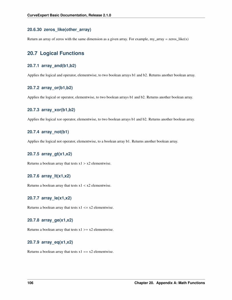
CurveExpert Basic Documentation, Release 2.1.0
20.6.30 zeros_like(other_array)
Return an array of zeros with the same dimension as a given array. For example, my_array = zeros_like(x)
20.7 Logical Functions
20.7.1 array_and(b1,b2)
Applies the logical and operator, elementwise, to two boolean arrays b1 and b2. Returns another boolean array.
20.7.2 array_or(b1,b2)
Applies the logical or operator, elementwise, to two boolean arrays b1 and b2. Returns another boolean array.
20.7.3 array_xor(b1,b2)
Applies the logical xor operator, elementwise, to two boolean arrays b1 and b2. Returns another boolean array.
20.7.4 array_not(b1)
Applies the logical not operator, elementwise, to a boolean array b1. Returns another boolean array.
20.7.5 array_gt(x1,x2)
Returns a boolean array that tests x1 > x2 elementwise.
20.7.6 array_lt(x1,x2)
Returns a boolean array that tests x1 < x2 elementwise.
20.7.7 array_le(x1,x2)
Returns a boolean array that tests x1 <= x2 elementwise.
20.7.8 array_ge(x1,x2)
Returns a boolean array that tests x1 >= x2 elementwise.
20.7.9 array_eq(x1,x2)
Returns a boolean array that tests x1 == x2 elementwise.
106 Chapter 20. Appendix A: Math Functions

CurveExpert Basic Documentation, Release 2.1.0
20.7.10 array_neq(x1,x2)
Returns a boolean array that tests x1 != x2 elementwise.
20.7.11 array_almost_eq(x1,x2, rtol, atol)
Tests two arrays x1 and x2, elementwise, to see if they are nearly equal within the tolerances specified in rtol andatol. Returns a boolean array. rtol is a relative tolerance, and atol is an absolute tolerance. To determine closeness,the relative difference rtol*abs(b) and the absolute difference atol are added together to compare against the absolutedifference between the elements of a and b.
20.7. Logical Functions 107

CurveExpert Basic Documentation, Release 2.1.0
108 Chapter 20. Appendix A: Math Functions

CHAPTER
TWENTYONE
APPENDIX B: MATH SYMBOL REFERENCE
21.1 Subscripts and superscripts
Command Result$alpha_i > beta_i$ αi > βi
$alpha^2 > beta_i^a$ α2 > βai
21.2 Fractions, binomials and stacked numbers
$\frac34$
34
$\binom34$ (34
)$\stackrel34$
34
$\frac5 - \frac1x4$
5 − 1x
4
21.3 Using parenthesis properly
$(\frac5 - \frac1x4)$
(5 − 1
x
4)
Notice how the parenthesis do not properly wrap the object inside. To address this, use the \left and \right qualifiers infront of your parenthesis.
109
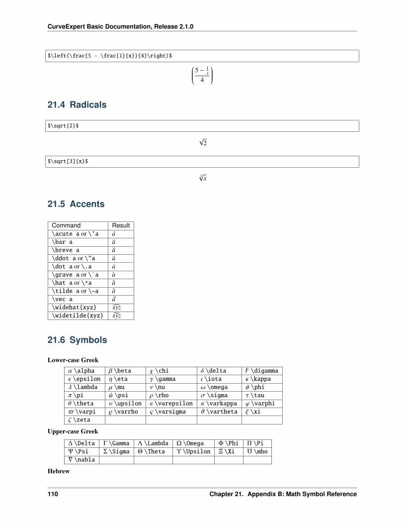
CurveExpert Basic Documentation, Release 2.1.0
$\left(\frac5 - \frac1x4\right)$ ⎛⎜⎜⎜⎜⎜⎝5 − 1x
4
⎞⎟⎟⎟⎟⎟⎠21.4 Radicals
$\sqrt2$
√2
$\sqrt[3]x$
3√x
21.5 Accents
Command Result\acute a or \'a a\bar a a\breve a a\ddot a or \"a a\dot a or \.a a\grave a or \`a a\hat a or \^a a\tilde a or \~a a\vec a ~a\widehatxyz xyz\widetildexyz xyz
21.6 Symbols
Lower-case Greekα \alpha β \beta χ \chi δ \delta z \digammaε \epsilon η \eta γ \gamma ι \iota κ \kappaλ \lambda µ \mu ν \nu ω \omega φ \phiπ \pi ψ \psi ρ \rho σ \sigma τ \tauθ \theta υ \upsilon ε \varepsilon κ \varkappa ϕ \varphi$ \varpi % \varrho ς \varsigma ϑ \vartheta ξ \xiζ \zeta
Upper-case Greek
∆ \Delta Γ \Gamma Λ \Lambda Ω \Omega Φ \Phi Π \PiΨ \Psi Σ \Sigma Θ \Theta Υ \Upsilon Ξ \Xi f \mho∇ \nabla
Hebrew
110 Chapter 21. Appendix B: Math Symbol Reference
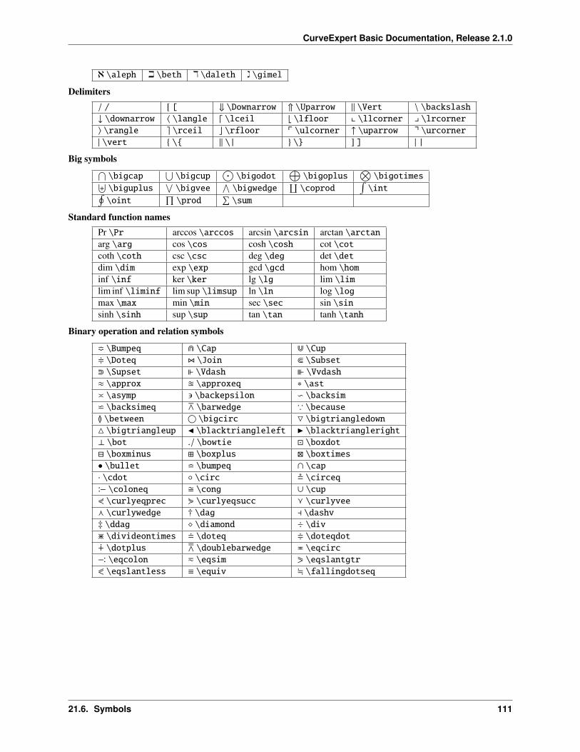
CurveExpert Basic Documentation, Release 2.1.0
ℵ \aleph i \beth k \daleth ג \gimel
Delimiters/ / [ [ ⇓ \Downarrow ⇑ \Uparrow ‖ \Vert ∖ \backslash↓ \downarrow ⟨ \langle ⌈ \lceil ⌊ \lfloor x \llcorner y \lrcorner⟩ \rangle ⌉ \rceil ⌋ \rfloor p \ulcorner ↑ \uparrow q \urcorner| \vert \ ‖ \| \ ] ] | |
Big symbols⋂\bigcap
⋃\bigcup
⨀\bigodot
⨁\bigoplus
⨂\bigotimes⨄
\biguplus⋁\bigvee
⋀\bigwedge
∐\coprod
∫\int∮
\oint∏\prod
∑\sum
Standard function namesPr \Pr arccos \arccos arcsin \arcsin arctan \arctanarg \arg cos \cos cosh \cosh cot \cotcoth \coth csc \csc deg \deg det \detdim \dim exp \exp gcd \gcd hom \hominf \inf ker \ker lg \lg lim \limlim inf \liminf lim sup \limsup ln \ln log \logmax \max min \min sec \sec sin \sinsinh \sinh sup \sup tan \tan tanh \tanh
Binary operation and relation symbols
m \Bumpeq e \Cap d \Cup+ \Doteq Z \Join b \Subsetc \Supset \Vdash \Vvdash≈ \approx u \approxeq * \ast≍ \asymp \backepsilon v \backsimw \backsimeq Z \barwedge ∵ \becauseG \between \bigcirc \bigtriangledown \bigtriangleup J \blacktriangleleft I \blacktriangleright⊥ \bot ./ \bowtie \boxdot \boxminus \boxplus \boxtimes∙ \bullet l \bumpeq ∩ \cap· \cdot ∘ \circ $ \circeqD \coloneq \cong ∪ \cup2 \curlyeqprec 3 \curlyeqsucc g \curlyveef \curlywedge † \dag ⊣ \dashv‡ \ddag \diamond ÷ \div> \divideontimes \doteq + \doteqdotu \dotplus [ \doublebarwedge P \eqcircE \eqcolon h \eqsim 1 \eqslantgtr0 \eqslantless ≡ \equiv ; \fallingdotseq
21.6. Symbols 111
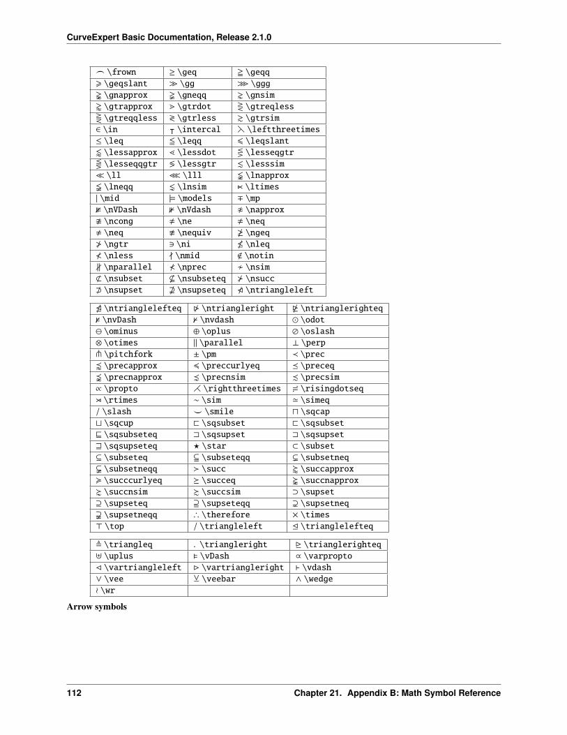
CurveExpert Basic Documentation, Release 2.1.0
_ \frown ≥ \geq = \geqq> \geqslant ≫ \gg ≫ \ggg \gnapprox \gneqq \gnsim' \gtrapprox m \gtrdot R \gtreqlessT \gtreqqless ≷ \gtrless & \gtrsim∈ \in ᵀ \intercal h \leftthreetimes≤ \leq 5 \leqq 6 \leqslant/ \lessapprox l \lessdot Q \lesseqgtrS \lesseqqgtr ≶ \lessgtr . \lesssim≪ \ll ≪ \lll \lnapprox \lneqq \lnsim n \ltimes| \mid |= \models ∓ \mp3 \nVDash 1 \nVdash 0 \napprox \ncong , \ne , \neq, \neq . \nequiv \ngeq≯ \ngtr ∋ \ni \nleq≮ \nless - \nmid < \notin∦ \nparallel ⊀ \nprec / \nsim1 \nsubset * \nsubseteq \nsucc2 \nsupset + \nsupseteq 6 \ntriangleleft
5 \ntrianglelefteq 7 \ntriangleright 4 \ntrianglerighteq2 \nvDash 0 \nvdash ⊙ \odot⊖ \ominus ⊕ \oplus ⊘ \oslash⊗ \otimes ‖ \parallel ⊥ \perpt \pitchfork ± \pm ≺ \precv \precapprox 4 \preccurlyeq ⪯ \preceq \precnapprox \precnsim - \precsim∝ \propto i \rightthreetimes : \risingdotseqo \rtimes ∼ \sim ≃ \simeq/ \slash ^ \smile ⊓ \sqcap⊔ \sqcup @ \sqsubset @ \sqsubset⊑ \sqsubseteq A \sqsupset A \sqsupset⊒ \sqsupseteq ? \star ⊂ \subset⊆ \subseteq j \subseteqq ( \subsetneq$ \subsetneqq ≻ \succ w \succapprox< \succcurlyeq ⪰ \succeq \succnapprox \succnsim % \succsim ⊃ \supset⊇ \supseteq k \supseteqq ) \supsetneq% \supsetneqq ∴ \therefore × \times⊤ \top / \triangleleft E \trianglelefteq
, \triangleq . \triangleright D \trianglerighteq⊎ \uplus \vDash ∝ \varproptoC \vartriangleleft B \vartriangleright ⊢ \vdash∨ \vee Y \veebar ∧ \wedge≀ \wr
Arrow symbols
112 Chapter 21. Appendix B: Math Symbol Reference
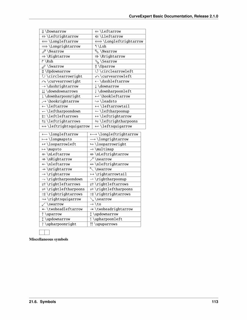
CurveExpert Basic Documentation, Release 2.1.0
⇓ \Downarrow ⇐ \Leftarrow⇔ \Leftrightarrow W \Lleftarrow⇐= \Longleftarrow ⇐⇒ \Longleftrightarrow=⇒ \Longrightarrow \Lsht \Nearrow v \Nwarrow⇒ \Rightarrow V \Rrightarrow \Rsh u \Searroww \Swarrow ⇑ \Uparrow \Updownarrow \circlearrowleft \circlearrowright x \curvearrowlefty \curvearrowright c \dashleftarrowd \dashrightarrow ↓ \downarrow \downdownarrows \downharpoonleft \downharpoonright ← \hookleftarrow→ \hookrightarrow \leadsto← \leftarrow \leftarrowtail \leftharpoondown \leftharpoonup⇔ \leftleftarrows ↔ \leftrightarrow \leftrightarrows \leftrightharpoons! \leftrightsquigarrow f \leftsquigarrow
←− \longleftarrow ←→ \longleftrightarrow↦−→ \longmapsto −→ \longrightarrow" \looparrowleft # \looparrowright↦→ \mapsto ( \multimap: \nLeftarrow < \nLeftrightarrow; \nRightarrow \nearrow8 \nleftarrow = \nleftrightarrow9 \nrightarrow \nwarrow→ \rightarrow \rightarrowtail \rightharpoondown \rightharpoonup \rightleftarrows \rightleftarrows \rightleftharpoons \rightleftharpoons⇒ \rightrightarrows ⇒ \rightrightarrows \rightsquigarrow \searrow \swarrow → \to \twoheadleftarrow \twoheadrightarrow↑ \uparrow \updownarrow \updownarrow \upharpoonleft \upharpoonright \upuparrows
Miscellaneous symbols
21.6. Symbols 113
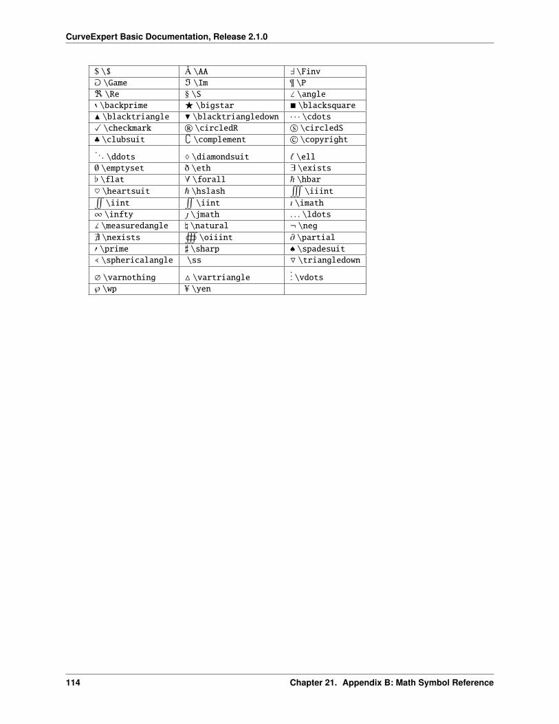
CurveExpert Basic Documentation, Release 2.1.0
$ \$ Å \AA ` \Finva \Game ℑ \Im ¶ \Pℜ \Re S \S ∠ \angle8 \backprime F \bigstar \blacksquareN \blacktriangle H \blacktriangledown · · · \cdotsX \checkmark r \circledR s \circledS♣ \clubsuit \complement © \copyright. . . \ddots \diamondsuit ` \ell∅ \emptyset ð \eth ∃ \exists[ \flat ∀ \forall ~ \hbar
\heartsuit \hslash#\iiint!
\iint!\iint ı \imath
∞ \infty \jmath . . . \ldots] \measuredangle \ \natural ¬ \neg
@ \nexists)\oiiint ∂ \partial
′ \prime ] \sharp ♠ \spadesuit^ \sphericalangle \ss O \triangledown
∅ \varnothing M \vartriangle... \vdots
℘ \wp U \yen
114 Chapter 21. Appendix B: Math Symbol Reference
CHAPTER
TWENTYTWO
APPENDIX C: THEORY
22.1 Linear Regression
Models which consist of a linear combination of a particular set of functions Xk are called linear models, and linearregression can be used to minimize the difference between the model and data. The general form of this kind of modelis
y(x) =∑
akXk(x)
where Xk(x) are fixed functions of x that are called the basis functions, and ak are the free parameters. Note that “linear”refers only to dependence of the model on the parameters ak; the functions Xk(x) may be nonlinear. Minimization ofthe above linear model is performed with respect to the merit function
S (a) =
n∑i=1
⎡⎢⎢⎢⎢⎢⎣yi −
np∑k=1
akXk(xi)
⎤⎥⎥⎥⎥⎥⎦2
The minimum of the above equation occurs where the derivative of S with respect to the parameters disappears.Substituting the linear model into this function, taking the first derivative, and setting this equal to zero gives thenormal equations that can be solved directly for the parameters ak.
22.2 Nonlinear Regression
22.2.1 Introduction
This program uses the Levenberg-Marquardt method to solve nonlinear regressions. This method combines thesteepest-descent method and a Taylor series based method to obtain a fast, reliable technique for nonlinear opti-mization. This statement will be repeated later, but can bear stating at the beginning of this discussion: neither ofthe above optimization methods are ideal all of the time; the steepest descent method works best far away from theminimum, and the Taylor series method works best close to the minimum. The Levenberg-Marquardt (LM) algorithmallows for a smooth transition between these two methods as the iteration proceeds.
22.2.2 Development
In general, the data modeling equation (with any number of independent variables) can be written as follows:
y = y(~x;~a)
The above expression simply states that the dependent variable y can be expressed as a function of the independentvariables ~x and vector of parameters ~a of arbitrary length. Note that using the ML method, any nonlinear equation
115
CurveExpert Basic Documentation, Release 2.1.0
with an arbitrary number of parameters can be used as the data modeling equation. Then, the merit function we aretrying to minimize is
χ2(~a) =
n∑i=1
(yi − y(~xi;~a)
σi
)2
where N is the number of data points, ~xi denotes the x data points, yi denotes the y data points, σi is the standarddeviation (uncertainty) at point i, and y(xi; a) is an arbitrary nonlinear model evaluated at the ith data point. This meritfunction simply measures the agreement between the data points and the parametric model; a smaller value for themerit function denotes better agreement. Commonly, this merit function is called the chi-square.
Now, we will take a step back to provide a framework of optimization methods. From the area of pure optimization,which will not be explained here, two basic ways of finding a function minimum are a Taylor series based method andthe steepest-descent method. The Taylor series method states that sufficiently close to the minimum, the function canbe approximated as a quadratic. Without detailed explanation of that method, a step from the current parameters a tothe best parameters amin can be written as
~amin = ~acur + H−1[−∆χ2(~acur)
]where H is the Hessian matrix (a matrix of second derivatives). If the approximation of the function as a quadratic is apoor one, then we might instead use the steepest-descent method, where a step to the best parameters from the currentparameters is
~amin = ~acur − c∆χ2(~acur)
This equation simply states that the next guess for the parameters is a step down the gradient of the merit function.The constant c is forced to be small enough that a small step is taken and the gradient is accurate in the region that thestep is taken.
Since we know the chi-square function, we can directly differentiate to obtain the gradient vector and the Hessianmatrix. Taking the partial derivatives of the merit function with respect to a gives
∂χ2
∂ak= −2
n∑i=1
yi − y(~xi;~a)σ2
i
∂y(~xi;~a)∂ak
To obtain the Hessian matrix, take the gradient of the gradient above (so that we have a matrix of partial secondderivatives):
∂2χ2
∂ak∂al= −2
n∑i=1
⎡⎢⎢⎢⎢⎣ 1σ2
i
∂y(~xi;~a)∂ak
∂y(~xi;~a)∂al
−yi − y(~xi;~a)
σ2i
∂2y(~xi;~a)∂al∂ak
⎤⎥⎥⎥⎥⎦Now, for convenience, define the gradient vector and the curvature matrix as
Gk = −12∂χ2
∂ak=
n∑i=1
⎡⎢⎢⎢⎢⎣yi − y(~xi;~a)σ2
i
∂y(~xi;~a)∂ak
⎤⎥⎥⎥⎥⎦Ckl =
∂2χ2
∂ak∂al=
n∑i=1
⎡⎢⎢⎢⎢⎣ 1σ2
i
∂y(~xi;~a)∂ak
∂y(~xi;~a)∂al
⎤⎥⎥⎥⎥⎦[Note that the second derivative term in C will be ignored because of two reasons: it tends to be small because it ismultiplied by (y − yi), and it tends to destabilize the algorithm for badly fitting models or data sets contaminated withoutliers. This action in no way affects the minimum found by the algorithm; it only affects the route in getting there.]So, the Taylor series method (inverse Hessian method) can be written as the following set of linear equations:
np∑k=1
Cklδal = Gk[1]
116 Chapter 22. Appendix C: Theory

CurveExpert Basic Documentation, Release 2.1.0
where NP is the number of parameters in the model that is being optimized. This linear matrix will be our workhorsefor this method after some modification; it can be solved for the increments da that, when added to the current approx-imation for the parameters, gives the next approximation. Likewise, we can substitute our “convenient” definitionsinto the steepest descent formula to obtain
δal = cGl[2]
Neither of the aforementioned optimization methods are ideal all of the time; the steepest descent method works bestfar away from the minimum, and the Taylor series method works best close to the minimum. The Levenberg-Marquardt(LM) algorithm allows for a smooth transition between these two methods as the iteration proceeds.
The first issue in deriving the LM method is to attach some sort of scale to the constant c in the steepest-gradientmethod (equation 2). Typically, there is no obvious way to determine this number, even within an order of magnitude.However, in this case, we have access to the Hessian matrix; examining its members, we see that the scale on thisconstant must be 1/Cll. But, that still may be too large, so let’s divide that scale by a nondimensional factor (l) andplan on setting this much larger than one so that the step will be reduced (for safety and stability).
The second issue to formulate the LM method is noting that the steepest-descent and Taylor series methods may becombined if we define a new matrix Mij by the following:
Mii = Cii(1 + λ), i = j
Mi j = Ci j, i , j
This matrix combines equations [1] and [2] into a convenient and compact form. So finally, we have a means ofcalculating the step da in the parameters by the following system of linear equations:
np∑k=1
Mklδal = Gk[3]
Note that when l is large, the matrix M is forced to be diagonally dominant; consequently, the above equation isequivalent to the steepest descent method (equation 2). Conversely, when the parameter l goes to zero, the aboveequation is equivalent to the Taylor series method (equation 1). So, we vary l to switch between the two methods,continually calculating a parameter correction da that we apply to our most recent guess for the parameter vector.
22.2.3 Procedure
The steps that are taken in the LM algorithm are as follows:
1. Compute χ2(a)
2. Pick a conservative value for λ (0.001 in CurveExpert)
3. Solve the linear equations (equation 3) for δa
4. Evaluate χ2(a + δa)
5. If χ2(a + δa) >= χ2(a), increase λ by a factor (10 in CurveExpert) and go back to step [3].
6. If χ2(a + δa) < χ2(a), decrease λ by a factor (10 in CurveExpert), correct the parameter vector by a = a + δa,and go back to step [3].
Iteration is stopped when |χ2(a + δa) − χ2(a)| < ε. This tolerance ε is the value specified by the user.
22.2. Nonlinear Regression 117

CurveExpert Basic Documentation, Release 2.1.0
118 Chapter 22. Appendix C: Theory
CHAPTER
TWENTYTHREE
APPENDIX D: REFERENCES
1. Bevington, Philip R., Data Reduction and Error Analysis for the Physical Sciences, 1969, McGraw-Hill, Inc.,Library of Congress QA278. B48.
2. Cleveland, William S.: “Robust locally weighted regression and smoothing scatterplots”, Journal of the Ameri-can Statistical Association, December 1979, volume 74, number 368, pp. 829-836.
3. Cleveland, William S., and Devlin, Susan J.: “Locally weighted regression: An approach to regression analysisby local fitting”, Journal of the American Statistical Association, September 1988, volume 83, number 403, pp.596-610.
4. Daniel and Wood, Fitting Equations to Data, 1971. Wiley & Sons, New York. Library of Congress QA297.D35.
5. Neter, Wasserman, and Kutner, Applied Linear Regression Models, 2nd ed. 1989, Irwin Press, Boston, MA.Library of Congress QA278.2 .N46.
6. Press, Flannery, Teukolsky, and Vetterling, Numerical Recipes in Pascal, 1989. Cambridge University Press,New York. Library of Congress QA76.73 .P2N87. Seber and Wild, Nonlinear Regression, 1989. Wiley & Sons,New York. Library of Congress QA278.2 .S425.
7. Ratkowsky, David A., Handbook of Nonlinear Regression Models. 1990. Marcel Dekker, Inc., New York.Library of Congress QA278.2 .R369.
8. Ratkowsky, David A., Nonlinear Regression Modeling: A Unified Practical Approach. 1983. Marcel Dekker,Inc., New York. Library of Congress QA278.2 .R37.
119

CurveExpert Basic Documentation, Release 2.1.0
120 Chapter 23. Appendix D: References

CHAPTER
TWENTYFOUR
INDICES AND TABLES
• genindex
• search
121

CurveExpert Basic Documentation, Release 2.1.0
122 Chapter 24. Indices and tables

INDEX
Aactivate, 4administrator, 3annotation, 44aspect, 72autoannotate, 44autofill, 17automated install, 3automatically plot, 72automatically update results, 69autoscale, 43, 45, 71autoscale lock, 43average, 21axis properties, 45
Bbackground, 48badges, 36bessel functions, 98bug, 68built-in math functions, 95
Ccache, 75calculate, 29calculation, 25, 27, 36clamp, 24clipboard, 76color coding, 35column labels, 18comma as decimal, 76comment, 17confidence bands, 38, 46confidence bounds, 45confidence level, 68constants, 95copy, 23, 45copy parameters, 37copy underlying data, 45copying graphs, 51copying result info, 37crop, 24
cursor, 22, 68curve data, 45curve fit, 29, 115CurveExpert Basic files, 18, 78CurveExpert files, 65curvefinder, 31custom, 30, 59, 61cut, 23CXP file, 65CXP files, 18, 78
Ddata, 21, 24data column labels, 18data file, 69data file location, 69data files, 15, 63, 76data operations, 24deleting results, 37delimiter, 69details, 37drag and drop, 37dragging, 44
Eelement, 44EMF, 51EPS, 51equation, 62equation display, 62equations, 107EULA, 84Excel, 68export, 65
Ffeatures, 1file locations, 84files, 69font, 72footer, 17formatting, 23functions, 59
123
CurveExpert Basic Documentation, Release 2.1.0
functions, array, 102functions, bessel, 98functions, comparison, 99functions, constants, 95functions, logical, 106functions, misc, 100functions, transcendental, 95
Ggetting started, 4graph properties, 45graph themes, 52graph toolbar, 42graphing, 39graphs and data pane, 7, 11guide, 4
Hheader, 17hiding panes, 8highlight, 72hotkeys, 52
Iimage, 44import, 15initial guesses, 30, 31, 70inserting rows, 23install, 3internet, 75interpolation, 28introduction, 1issues, 68
JJPEG, 51
Llegend, 44, 50legend order, 51legend properties, 50Levenberg-Marquardt, 115license, 3, 4, 84licensing (third party), 86line data, 45line properties, 46linear regression, 29, 115localization, 74, 76locator, 44log viewer, 83logging, 73, 74logs, 83
Mmarker properties, 46math functions, 95math symbols, 107mathtext, 52, 62, 72, 107mathtext reference, 52maximize, 8memory, 75menu reference, 12menus, 8messages pane, 7, 11models, 29, 30, 59multicore, 11multiple instances, 83
NNIST, 79nonlinear regression, 29, 115numeric format, 76
Oonline, 75operating on data, 24overall graph properties, 48
Ppan, 43, 72panes, 7paste, 23PDF, 51pi, 95pick, 44, 72plot toolbar, 42PNG, 51polynomial, 29prediction bands, 38, 46prediction bounds, 45preview pane, 7, 11print, 44printing, 52, 65, 72printing graphs, 52proxy, 75PS, 51purchase, 4
Qquerying results, 37
RRAW, 51reading data files, 15redo, 23redraw, 72
124 Index
CurveExpert Basic Documentation, Release 2.1.0
references, 117region settings, 76removing columns, 23removing results, 37removing rows, 23reports, 68reserved words, 62residual, 70restore, 8result badges, 36result color coding, 35result details, 37result icons, 35result pane, 7result preview, 37results, 34results pane, 10results update, 36RGBA, 51rotate, 24
Ssave graph, 44saving data, 63saving graphs, 51, 65scale, 24shortcuts, 52silent install, 3simple, 61sort, 24, 68splines, 28spreadsheet, 21, 68standard deviation, 21standard math operations, 62statistics, 21status bar, 11subscript, 107superscript, 107surface properties, 46SVG, 51system administrator, 3
Ttable, 45tension splines, 28themes, 52theory, 115TIFF, 51tips, 67title, 48tolerance, 28, 70toolbar, 9, 42toolbar reference, 9transform, 24
translate, 24trial, 3
Uundo, 23, 75updating results, 36user interface, 6
Vvalidation, 79verification, 78
Wweighting, 29, 30window menu, 8windows, 3writing data, 63
Xxy plot, 41
Zzoom, 43
Index 125