customer concentration and loan contract terms* · customer concentration and loan contract terms*...

Electronic copy available at: http://ssrn.com/abstract=2442314

Customer Concentration and Loan Contract Terms*

Murillo Campello Janet GaoCornell University & NBER Cornell University

[email protected] [email protected]

This Draft: May 27, 2014

Abstract

Recent research shows that firms enjoy operating efficiencies when dealing with fewer, larger cus-

tomers. It ignores, however, how firms’ creditworthiness is affected by their large exposure to these

customers. We look at multiple contractual features of bank loans to gauge how the credit market

evaluates a firm’s customer base. We first model how interactions between firms and their major

customers influence bank loan terms. Empirically, we find that higher customer concentration leads

to increases in interest rate spreads and in the number of restrictive covenants featured in bank loans.

Customer concentration also reduces the maturity of those loans. The duration and depth of the

relationship between firms and their banks are further negatively affected by increased customer con-

centration. All of these effects are aggravated by a deterioration in customers’ financial conditions

(controlling for firms’ own finances, their industry, and the identity of their banks). Our results show

that in spite of the fact that customer concentration contributes to profitability, it ultimately bears

negative consequences for corporate credit. The analysis provides insights about integration along

the supply chain and the limits of the firm.

Key words: Customer Concentration, Bank Loans, Contract Terms, Financial Distress, Instrumental

Variables, Fixed Effects.

JEL classification: G21, G30, G32.

*We are thankful for Edward Fee and Erasmo Giambona for sharing their data with us. We also

thank Jean-Noel Barrot, Sudipto Dasgupta, Tomislav Ladika, Rafael Matta, and Justin Murfin for

their comments.


Customer Concentration and Loan Contract Terms

Abstract

Recent research shows that firms enjoy operating efficiencies when dealing with fewer, larger cus-

tomers. It ignores, however, how firms’ creditworthiness is affected by their large exposure to these

customers. We look at multiple contractual features of bank loans to gauge how the credit market

evaluates a firm’s customer base. We first model how interactions between firms and their major

customers influence bank loan terms. Empirically, we find that higher customer concentration leads

to increases in interest rate spreads and in the number of restrictive covenants featured in bank loans.

Customer concentration also reduces the maturity of those loans. The duration and depth of the

relationship between firms and their banks are further negatively affected by increased customer con-

centration. All of these effects are aggravated by a deterioration in customers’ financial conditions

(controlling for firms’ own finances, their industry, and the identity of their banks). Our results show

that in spite of the fact that customer concentration contributes to profitability, it ultimately bears

negative consequences for corporate credit. The analysis provides insights about integration along

the supply chain and the limits of the firm.

Key words: Customer Concentration, Bank Loans, Contract Terms, Financial Distress, Instrumental

Variables, Fixed Effects.

JEL classification: G21, G30, G32.


1 Introduction

U.S. manufacturers attribute, on average, over one-third of their sales figures to a few major

customers, and the level of customer concentration is increasing in recent years. A concentrated

customer base is cited as a positive factor in analyst reports, management forecasts, and

even IPO prospectuses, as it is believed to enhance firms’ profitability by reducing overhead

costs. Notably, such arguments find support in recent academic research (e.g., Patatoukas

(2012) and Irvine et al. (2013)). Relying on major customers has shortcomings, nonetheless.

Major customers demand lower prices, purchase irregularly, and delay payments (Fee and

Thomas (2004), Kelly et al. (2013), Murfin and Njoroge (2013), and Barrot (2014)).1 While

these problems are shown to be important, the literature has not examined whether a close

association with fewer, larger customers expose firms to costs and risks that affect their access

to credit.

This paper examines how the credit market evaluates a firm’s customer-base profile, char-

acterizing how customer concentration and financial status affect the firm’s access to funds. To

do so, we look at multiple features of bank loan contracts and firm–bank relationships. This

approach allows us to assess how informed lenders modify the terms of their credit offerings in

response to the evolving nature of firms’ customer-base profile and supply-chain relations. We

first model the interplay between customer concentration, firm investment choices, and loan

contract terms in a simple theoretical framework. The model we develop is useful in providing

clear predictions about relations that can be taken to the data. We then empirically examine

the impact of customer concentration on several features of loan contracts, including interest

rate spreads, maturity, and the number of restrictive covenants. We also examine the impact

of customer concentration on the length and depth of the relationships between firms and their

banks. Our results are new to the literature in revealing contracting costs associated with in-

creased reliance on few, large customers. We show that these costs are significant and manifest

themselves along various dimensions, pointing to important limitations to deeper integration

among firms along their supply chain.

1These behaviors have attracted attention from the press, with reports that large, powerful firms such asWalmart and P&G “abuse” their suppliers by delaying payment on their products. See Wall Street Journalarticle: “Small Firms’ Big Customers Are Slow to Pay” (June 6, 2012).

1

In a nutshell, our model characterizes firms’ incentives to invest in projects that enhance

relations with their suppliers, showing how this affects their credit. Relationship-specific in-

vestments have been described in the existing theoretical and empirical literatures (e.g., Klein

et al. (1978), Hart (1995), Bolton and Scharfstein (1998), Kale and Shahrur (2007), and Baner-

jee et al. (2008)). These projects may involve investment in R&D, unique fixed assets, and

modifications of standard production processes. Relationship-specific projects are less desir-

able from lenders’ perspective because their uniqueness engenders higher risks and lower resale

values in liquidation. Our equilibrium analysis shows that the higher the importance of major

customers, the greater the gains from relationship-specific investments, and the lower the credit

quality of firms undertaking those investments. The model implies, among other things, that

increases in firms’ customer concentration will cause their banks to impose costlier, stricter

loan contract terms.

To test our model’s predictions, we gather information on bank loan terms from LPC–

Dealscan and merge that information with data on firm customers from Compustat’s Segment

Database over the 1985–2010 window. Our baseline results can be summarized as follows. A

more concentrated customer base increases both the interest rates and the number of restrictive

covenants featured in bank loans. Customer concentration also reduces the maturity of those

loans. These effects are statistically and economically significant. Controlling for bank identity,

industry effects, macroeconomic conditions, and firm characteristics, a one-standard-deviation

increase in customer concentration leads to 10 basis points higher interest spreads on new

bank loans; this compared to an average spread of 173 basis points. The same shift leads to,

on average, 0.2 additional loan covenants; compared to the sample mean of 1.8 covenants. It

also leads to a reduction in loan maturity by 2 months; compared to average maturity of 45

months. The magnitudes of these effects are significant given the high level of competition in

the market for corporate lending.

We also examine whether customer concentration affects the length and depth of a firm’s

banking relationships. We find that a one-standard-deviation increase in customer concentra-

tion leads to 0.3 fewer loans from the firm’s current bank in the future, and 0.4 years shorter

relationship with that bank. These magnitudes are significant compared to the sample average

levels of 4.2 future loans and 2.9 future years of relationship.

2

Observed relations between customer concentration and borrowing terms can be biased

due to omitted variables. In particular, it can be argued that unobserved characteristics might

lead a firm’s customer concentration to increase and its credit terms to deteriorate — this,

despite of a positive relation between customer concentration and profitability. To alleviate

such concerns, we experiment with the use of data on M&A activity in customers’ industries

(downstream mergers) as an instrument for customer concentration. Downstream M&A ac-

tivity is a plausible instrument for two reasons. First, it is related to customers’ own growth

prospects (Fee and Thomas (2004) and Erel et al. (2014)) and following merger deals in

customer industries, suppliers are likely to face higher customer concentration (inclusion re-

striction). Second, that activity is unlikely to affect suppliers’ borrowing terms through chan-

nels other than customer–supplier linkages (exclusion restriction). Bearing in mind concerns

that industry-level, time-varying dynamics could influence customers’ M&A activity and firms’

credit terms, we further control for industry-year-fixed effects in our tests. Our IV estimations

imply that following high levels of M&A activity in customer industries, supplier firms observe

higher customer-base concentration, which then lead to costlier, stricter borrowing terms and

shorter banking relationships.

We dig deeper into the meaning of our results by examining whether the financial condi-

tions of a firm’s large customers affect its credit terms. Customers in worse financial shape

may, for example, face difficulties in maintaining purchase agreements and paying on time,

eventually burdening their suppliers. Confirming the logic of our argument, we find that loan

spreads increase even more and the number of covenants is even higher when a firm’s large cus-

tomers are likely to be distressed (as proxied by measures such as distance-to-default). Large

customers’ financial distress further reduces a firm’s loan maturity and the length and depth

of its banking relationships.

Our empirical investigation further characterizes the channels through which customer con-

centration affects the credit terms offered by banks. As highly-regulated intermediaries, banks

are particularly concerned about loan failures. If higher customer concentration is associ-

ated with higher loan failure rates for supplier firms, banks will naturally impose stricter

loan terms. To establish this link, we identify loan failures by matching our data with the

LoPucki bankruptcy database, which has records of corporate failures. We find a positive,

3

significant relation between customer concentration and supplier loan failure rates. To wit, a

one-standard-deviation increase in customer concentration is associated with a 2 percentage

points increase in loan failure rate. The impact is sizable when compared to the sample average

loan failure rate of 6.5 percent. Our results show direct evidence that customer concentration

is an important concern for banks’ decisions to offer corporate credit. They identify the cause

of that concern and gauge its consequences across various dimensions of loan contracting.

Our paper is related to various strands of literature. First, it speaks to a growing literature

on the relation between customer concentration and profitability. Patatoukas (2012) argues

that having large customers helps firms achieve economies of scale by lowering overhead costs.

Irvine et al. (2013) further show that the beneficial effects of customer concentration vary

according to suppliers’ size and age. Fee and Thomas (2004) report that customers gain ad-

ditional bargaining power over suppliers after horizontal mergers, and that this is reflected

in stock prices. Greene et al. (2013) show that when customers become more powerful they

demand better trade terms. Our study contributes to this literature by showing the responses

from credit markets to changes in customer concentration. Like previous papers, we show

that customer concentration is indeed associated with higher firm profitability. Using lenders’

perspective, however, we show that concentrated customer bases ultimately have negative im-

plications for firm creditworthiness, leading banks to impose costlier, stricter loan terms.

Our study is also related to existing work on how supply-chain relationships affect firms’

financial policies. Titman and Wessel (1988) and Banerjee et al. (2008) argue that firms

tend to procure more unique assets when they rely on major customers. These firms have

lower leverage ratios because customer liquidation imposes high redeployment costs for their

relationship-specific assets (see also Kale and Shahrur (2007)). Hennessy and Livdan (2009)

model a firm’s leverage based on trade-offs between gains from bargaining power against sup-

pliers and costs associated with lower input quality. We add to this research by showing how

different features of debt contracting — e.g., interest rates, maturity, and covenants — relate

to firms’ customer base.

Our paper is also related to the literature on credit contagion along the supply chain. Ex-

isting studies show that a firm’s financial distress can impact its suppliers and customers (e.g.,

Kolay et al. (2012)). In that vein, Cohen and Frazzini (2008) report that customers’ earnings

4

surprises are incorporated into suppliers’ stock prices. Consistent with these studies, our find-

ings show that financially-distressed customers can generate severe negative externalities for

their suppliers; in particular, have detrimental consequences for their borrowing.

Finally, our study is related to the literature on the determinants of bank loan terms (ex-

amples are Graham et al. (2008), Roberts and Sufi (2009), Lin et al. (2011), Hertzel and

Officer (2012), Valta (2012), and Cen et al. (2014)). Closer to our study, Valta finds that

firms in competitive industries face higher loan spreads because competition increases cash

flow risk. Hertzel and Officer report that firms face higher spreads following industry-rivals’

bankruptcies, especially in competitive industries. Cen et al. find that supply-chain relations

may reduce informational asymmetries between banks and firms in the long run. None of these

papers consider the effect of customer concentration or distress on loan terms.

The paper proceeds as follows. Section 2 contains our theoretical motivation for the in-

terplay between customer concentration and firm credit terms. Section 3 describes our data

and methodology. Section 4 reports univariate analyses. Section 5 describes our baseline re-

sults. Section 6 reports our instrumental variable analysis. Section 7 explores cross-sectional

differences in the effect of customers’ financial health on suppliers’ borrowing terms. Section 8

describes a case study of credit contagion inside the supply chain. Section 9 reports a direct

test of the effect of customer concentration on bank loan failure rates. Section 10 concludes.

2 A Model of Customer Concentration and Bank Credit

We analyze the relation between a firm’s customer concentration and bank credit using a

simple theoretical framework. In it, we model the interplay between the customer, the supplier

firm, and its bank, keeping the focus on the dynamics we want to study empirically. We do not

model industry dynamics. In turn, we implicitly take customer concentration as given, reflect-

ing the crux of our supply-chain-based story for a potentially deep association between a firm

and its major customer. A major customer in our model may develop a deep relationship with

a particular supplier to the point of shaping that firm’s investment choices. This differentiates

that firm from other producers in its industry. The model delivers several testable implications.

5

2.1 Setting

The base model contains a firm, a major customer, and a bank (we allow for multiple firms

and firm heterogeneity below). The firm has to make investment decisions that maximize its

profits, choosing between projects with different profiles.

The model has two periods and at t = 0, the firm faces two mutually exclusive projects.

Both projects require initial investment I and have a payoff at t = 1. The firm has no funds,

so it borrows capital from the bank. Project A is risky. It pays αI with probability p, and 0

with probability 1− p. Project B is safe and pays βI with probability 1 (α < 1 < β).

To make the problem interesting, project choice may have different impacts on the firm’s

relations with its major customer and bank. Project B gives a higher expected return; that is,

β > pα. That project can be thought of as a standard technology with ex-ante known ability

to generate stable cash flows and with high resale value; this is the project that is preferred by

the bank. Project A, in contrast, engenders relationship-specific investments the firm makes

to fulfill the needs of its major customer. The relationship-specific investment can involve

expenditures with R&D, unique fixed assets, customization, and modifications to standard

production processes. Project A is riskier for the firm because it has lower success rate and lower

resale value. At the same time, it creates synergistic benefits for the firm’s major customer that

are ultimately shared by the firm.2 The major customer derives value VA from project A and

VB from project B, and we assume that it prefers the relationship-specific project pαVA > βVB.

At t = 1, the firm sells a proportion µ of its output to the major customer; 1 − µ is sold

to a set of small customers. The major customer can observe the firm’s project choice. To

motivate the firm to take project A, the major customer offers different prices for different

project outputs. For simplicity, we assume the non-major customers pay a price 1 per unit of

output for either projects, while the major customer offers δA per unit for project A and δB per

unit for project B; where δA > δB. This price schedule is the outcome of bargaining between

the firm and the major customer. It reflects the terms in the sales contract agreed upon by

the parties and it is binding. It can include future transaction prices, speeds of payment, and

can also reflect variations in overhead costs during the production process.3

2Neither the major customer nor the supplier necessarily belongs to a perfectly competitive industry, andneither has absolute bargaining power against the other.

3We assume that the relationship-specific investment does not impact the sales price to firm’s non-major cus-

6

2.2 Base Analysis

To ease the exposition, we momentarily assume that there is no asymmetry of information

between the bank and the firm. The bank can observe the amount the firm borrows I, its choice

of project, and its customer concentration µ. The bank also knows that the firm will default

on its loan payment at t = 1 with probability 1 − p if it chooses project A. Accordingly, the

bank imposes rate R = 1p

if the firm chooses the risky project and risk-free rate r (1 ≤ r ≤ β)

if the firm chooses the safe project. The firm chooses between the two projects to maximize

its total value at t = 1 given bank rates R and r as follows:

max{pα(µδA + 1− µ)I −RI, β(µδB + 1− µ)I − rI} (1)

The firm will choose to invest in project A if pα(µδA+1−µ)−R > β(µδB+1−µ)−r. Simplifying

this condition, the firm chooses project A if the customer’s offer satisfies the following:

pαδA − βδB >(1− µ)(β − pα) +R− r

µ. (2)

The major customer will also benefit from project A if the following holds:

pα(VA − δA) > β(VB − δB). (3)

Therefore, the firm and its major customer will be in agreement and choose project A if:

(1− µ)(β − pα) +R− rµ

< pαδA − βδB < pαVA − βVB. (4)

Conversely, project B will be chosen if:

(1− µ)(β − pα) +R− rµ

> pαδA − βδB > pαVA − βVB. (5)

The conditions above make it clear that for high levels of customer concentration µ (that is,

µ > β−pα+R−rβ−pα−βVB+pαVA

), the firm and the customer will agree on the relationship-specific invest-

ment, project A; for low levels of µ, the standard project B will be selected.

tomers. Non-major customers do not have the ability to change the price or to delay their payments to the firm.

7

2.3 Firm Heterogeneity

To make the model realistic and deliver testable predictions, we allow for many firms in the

economy. Moreover, we allow firms to be heterogeneous in their ability to successfully invest

in the relationship-specific (risky) project. Finally, we relax the assumption that banks have

perfect information about firms. Instead, we only assume that banks can observe (ex-post)

firms’ project choice, and that they know the general distribution of “firm quality” (ability

to succeed in the relationship-specific project). We avoid clutter in the model’s notation by

associating the distribution of firm quality with the success probability parameter p, denoting

F (p) as a function of p ⊂ [p, p]. The parameter p (p) is the lowest (highest) probability of

success in the distribution F (p).

In this economy, banks set loan prices based on the expected probability of default. This

captures the fact that commercial banks are subject to regulatory capital requirements and

cannot diversify away the default risk of their loans. We assume a perfectly competitive bank-

ing market. Without loss of generality, we model the lending decision of only one bank.

We take that major customers have private information about their needs for customiza-

tion and know their suppliers’ ability to successfully deliver the relationship-specific project

A. This reflects the common assumption in the literature that major customers have infor-

mation advantage over banks regarding real investment projects their suppliers implement, as

customers can better understand input transactions, and trade credit works as a monitoring

tool (Biais and Gollier (1997) and Burkart and Ellingsen (2004)). Major customers uniformly

prefer project A; which is equivalent to: pαVA > βVB.

It follows that for every level of customer concentration µ, a separating equilibrium exists

where there is a threshold value p∗ such that the “better firms” (those whose p > p∗) will

choose the risky project and the “worse firms” (whose p < p∗) will choose the safe project. Ac-

cordingly, the bank charges a break-even rate R = 1E[p|p≥p∗] if the firm takes the risky project,

and the risk-free rate r if the firm takes the safe project. The only condition needed for this

equilibrium is that the better firms do not want to take the safe project and the worse firms

do not want to take the risky project:

pα(µδA + 1− µ)−R > β(µδB + 1− µ)− r, ∀p > p∗ (6)

8

pα(µδA + 1− µ)−R < β(µδB + 1− µ)− r, ∀p < p∗. (7)

Note that R decreases with p∗ ( ∂R∂p∗

< 0), suggesting that when the bank knows only good firms

undertake the risky project, it is less worried about default. The bank will thus charge a lower

interest rate.

The equilibrium threshold p∗ will satisfy the following break-even condition:

(1− µ)(β − p∗α) +R− rµ

= p∗αVA − βVB. (8)

This expression describes the trade-off between projects for the marginal firm. The left-hand

side presents the cost of undertaking the risky project. The first term captures the loss of sales

to the non-major customers, while the other terms capture the additional cost (mark up) of the

bank loan. The right-hand side presents the benefit of undertaking the risky project, which is

also the maximum level of “inducement” the major customer could offer. The threshold value

p∗ is determined by equating the costs to the benefits of project A for the firm.

Eq. (8) can be written as F = (p∗αVA − βVB)µ + (p∗α − β)(1 − µ) − (R − r). Given

∂R∂p∗

< 0, it follows that ∂F∂p∗

> 0 and ∂F∂µ

> 0. Using the Implicit Function Theorem, we have

that ∂p∗

∂µ< 0, which implies that the quality of firms taking the risky project declines with

customer concentration. Put differently, a higher level of customer concentration, µ, prompts

more firms to invest in the relationship-specific project A (lower p∗), prompting the bank to

charge a higher mark up interest rate (R− r).

2.4 Customer Financial Condition

It is natural to consider a firm’s major customer’s financial condition as a concern to banks

in this setting. We extend the model to shed light on how customers’ financial heath affects

contracting.

Assume at t = 1, there is a probability 1−λ that the major customer experiences financial

difficulty and cannot pay the supplier firm. When a major customer is in financial distress, the

supplier can still sell the output from its projects to other customers at price 1. This means

that the firms who take project A receive α with probability 1 − λ and the full output price

δAµα+(1−µ)α with probability λ. The firms that undertake project B receive δBµβ+(1−µ)β

9

with probability λ and β with probability 1− λ.

From the above setting, we can see that if the firm takes project A, it will default on its

bank loan when the customer fails to pay. However, if the firm takes project B, it will not

default, since β ≥ r ≥ 1 > α. To make the problem more realistic, we also allow for some

degree of loan recovery when the firm is driven to default by its customer. We assume that

the bank can recover the supplier’s assets and resell them at a discount cost. Accordingly, we

denote the recovery rate to be η, 0 < η ≤ 1. Therefore, the bank’s break-even rate R given

(p, λ, µ) is determined by pλR + ηpα(1− λ)(1− µ) = 1, or

R =1− ηpα(1− λ)(1− µ)

pλ=

1− ηpα(1− µ)

pλ+ ηα(1− µ). (9)

Similar to the case without customer distress, a separating equilibrium exists in this setting.

In this equilibrium, the better firms (p > p∗) take project A and the worse firms (p < p∗) take

project B. The threshold p∗ satisfies the following condition:

p∗αVAµ− βλVBµ = p∗λR− r + β((1− µ)λ+ 1− λ)− λp∗α(1− µ). (10)

One can solve for p∗ as follows:

p∗ =βλVBµ+ β((1− µ)λ+ 1− λ)

αVAµ− λR + αλ(1− µ). (11)

We prove in Appendix B that the bank will charge a “fair” rate R if it observes a firm

undertake project A:

R =1− ηE[p|p > p∗]α(1− µ)

E[p|p > p∗]λ+ ηα(1− µ). (12)

We also show in Appendix B that dp∗

dλ> 0, dE[p|p>p∗]

dλ> 0, and ∂R

∂λ< 0.

Our goal is to understand the relationship between R and customer’s financial health λ. In

this regard, the relation dp∗

dλ> 0 is important as it shows that a higher customer distress risk

causes lower quality firms to choose project A. This seemingly counter-intuitive result arises

from firms’ increased risk-shifting incentives given the higher likelihood of default. With a

10

higher probability of financial distress, the major customer needs to pay more to induce the

supplier to undertake project A. The supplier thus faces a compensation scheme that involves

a large payment from the customer when it is in good financial shape, but no obligations

otherwise (due to limited liability).

This analysis helps us establish that the financial health of the customer influences the

borrowing cost of the supplier. When the customer is in good financial condition, the supplier

is offered more favorable contract terms. If the customer is in poor financial shape, however, the

supplier has even higher incentives to risk-shift, and the bank imposes higher borrowing costs.

2.5 Empirical Predictions

The model delivers very direct empirical implications and it is worth collecting them in a

subsection. As µ increases, the firm’s payoff depends more on its large customer. That large

customer can therefore more easily “induce” the firm to undertake the relationship-specific,

risky project. For larger µ, even firms with low ability will choose the risky project. It follows

that the threshold p∗ declines with customer concentration. A lower threshold p∗ indicates

higher overall failure rates for firms that choose to conduct relationship-specific projects. An-

ticipating the higher default rates that are associated with those projects, the bank will require

costlier, stricter terms for its loans. We write these predictions as follows:

Hypothesis 1 Banks will impose costlier, stricter loan contract terms on firms with higher

customer-base concentration.

Hypothesis 2 Firms with higher customer-base concentration experience higher loan failure

rates.

Hypothesis 3 Banks will impose costlier, stricter loan contract terms on firms that face cus-

tomers in worse financial conditions.

Our model reconciles the evidence that firms with more concentrated customer bases are

more profitable (Patatoukas (2012)) with the observation that those relationships are inher-

ently risky and may prompt default and bankruptcy along the supply chain (Hertzel et al.

(2008) and Kolay et al. (2012)). Simply put, establishing deeper relationships with major

11

customers can be both profitable and risky. The model shows that the risk is passed on to the

bank, which in turn responds by offering loan menus with costlier, stricter terms.

Note that the model focuses on a general notion of firms’ “borrowing costs” for simplicity.

The intuition easily extends to various features of standard loan terms, including interest rate

spread, maturity, and the presence of restrictive covenants. Making these contract features

costlier and stricter for the firm is meant to deter risk-taking. Our empirical tests will revolve

around each of these observable outcomes: loan markups, loan maturity, loan covenants, and

loan failures. We will also examine how customer concentration affects derivative measures of

the relationship between supplier firms and their banks: depth and duration.

3 Sample Construction and Empirical Methodology

We identify firms’ major customers using Compustat’s Segment Customer database. State-

ment of Financial Accounting Standard (SFAS) No.14 requires firms to report all customers

that represent more than 10% of a firm’s total sales. The Segment database collects customer

information including the names of the customers and their assigned sales figures. In identify-

ing important customer relations, we focus on recurring customers and exclude customers that

appear for fewer than three times for a firm in the sample period. We focus on manufacturers

(SIC 2000–3999) to ease comparisons across firms and because firms operating in this sector

resemble our supply-chain story more closely. Notably, information from the U.S. input/output

matrix suggest that supplier–customer links in the manufacturing sector feature firms on both

ends of the relationship.4

We extract bank loan contract information from LPC–Dealscan from 1985 through 2010,

and link loan-level data to Compustat firm identifiers following Chava and Roberts (2008). We

examine revolvers and term loans since both types of loans provide information on the pricing

and the restrictiveness of bank credit.

We construct our final sample by combining the customer and bank loan information. For

a firm to be included in the sample, we require it to have available customer information, loan

characteristics, and information on standard variables such as size, leverage, and market-to-

4Over two-thirds of output in those industries is sold as intermediary goods to other manufacturers, theremainder goes to bulk retailers.

12

book. We glean into how banks update loan pricing and other contracting features by focusing

on newly initiated (or renegotiated) loans during the year when the firms report customer

information. Notably, following prior literature (e.g., Campello et al. (2011), Lin et al. (2011),

and Hertzel and Officer (2012)), we do not repeatedly account for the same loans for the years

after initiation. As a result, our dataset has a panel structure in which individual firms appear

sparsely (more on this shortly).5

3.1 Customer Concentration

The unit of observation in the Segment database is a supplier–customer pair. For each

supplier, we aggregate all available customer information and define customer concentration

in two ways.

Our first measure of customer concentration is based on the percentage of sales that a firm

assigns to its major customers (similar to Banerjee et al. (2008)). In particular, we define Cus-

tomerSales as the sum of the percentage sales to the set of customers the firm reports as “major

customers” (i.e., those at least 10% of total sales). CustomerSales is computed as follows:

CustomerSalesi =

ni∑j=1

%Salesij,

where ni is the number of firm i ’s major customers, and %Salesij = Sales of i to jTotal Sales of i

, is the per-

centage sales from firm i to customer j over all i ’s sales. A high level of CustomerSales means

a large proportion of a firm’s sales go to its major customers. Accordingly, a small group of

buyers may ultimately influence the firm’s investment and profitability.

Our second measure is the sales-weighted size of a firm’s major customers. This measure

is more nuanced than the first in that it gives more importance to larger customers that also

happen to be larger firms, which presumably might have more bargaining power. We define

CustomerSize as the size of major customers, weighted by the firm’s percentage sales to these

5We further identify firms whose customers also borrow from their same banks. These firms account for4% of borrowers in our sample and excluding them does not change our results.

13

customers. CustomerSize is computed as follows:

CustomerSizei =

ni∑j=1

%Salesij × Sizej,

where Sizej is the size (defined by log of total assets) of customer j. A high level of Customer-

Size means that a firm relies more heavily on a few, large-sized customers.

3.2 Borrowing Terms

Chava and Roberts (2008), Roberts and Sufi (2009), and Campello et al. (2011) describe

the elements of the LPC–Dealscan dataset that are relevant for our analysis. We follow the

methodology in Campello et al. and measure three contract features of bank loan terms. The

first is loan spread (LoanSpread). LoanSpread is the “All-in-Drawn” spread (in basis-points)

over LIBOR. “All-in-Drawn” spread is computed as the sum of coupon and annual fees on

the loan in excess of six-month LIBOR. The second feature is loan maturity (LoanMaturity).

LoanMaturity is the number of months until maturity. Finally, we count the total number of

restrictive covenants present in the loan facility (LoanCovenants).

3.3 Banking Relationships

In addition to changing loan terms, banks can also react to a firm’s customer concentration

by terminating their relationships with the firm. If customer concentration is related to exces-

sive credit risk or undesirable investment choices, banks can stop extending loans to the firm,

terminating their relations. We design empirical measures of banking relationships to capture

these dynamics.

Each time a firm discloses its customer concentration, we look forward in the sample window

searching for subsequent loan arrangements (renewed relations in the future) with its current

banks. We measure these future banking relations using two methods. First, we measure the

length of the future banking relationship as the number of years in which the bank continues to

lend to the firm in the future (FutureDuration). For each bank loan contract, FutureDuration

counts the number of years until the last occurrence of the firm receiving a loan from the

current bank. Higher values of FutureDuration suggest that the bank and the firm maintain

14

relations for a long period after the disclosure of information about customer concentration.

Our second measure of banking relationship is the additional loans extended by the bank to

the firm after the information of customer concentration (FutureLoans). FutureLoans is defined

as the number of loans issued by the same bank after the current loan. Similar to FutureDu-

ration, FutureLoans measures a bank’s commitment to the lending relationship. However, it

emphasizes the intensity rather than the length of the relationship.

Naturally, both measures of banking relationships suffer from attrition bias, in that we

observe shorter future duration and fewer future loans as we approach the end of the sample.

We therefore restrict our banking relationship tests to fiscal years prior to 2007, leaving at

least 5 years, which is above the 85th percentile of the length of future banking relationships

in our sample.6

3.4 Loan Failures

To corroborate our argument that a more concentrated customer base is associated with

worse creditworthiness, we examine the relation between loan failure rates and customer con-

centration. If customer concentration is associated with a higher likelihood of loan failure,

banks will naturally impose stricter loan terms ex-ante.

We examine this conjecture by using bankruptcy data from the LoPucki database, which

provides detailed bankruptcy filings over the 1980–2012 window.7 We match the LoPucki

bankruptcy data with bank loan information, and identify a loan failure event if the borrower

files for bankruptcy prior to an existing loan maturity date. For this case, we assign an indicator

variable LoanFailure to 1. If there is no bankruptcy before the maturity of the loan, then

LoanFailure = 0. Finally, we match the loan failure variable with firms’ customer information.

3.5 Empirical Methodology

We estimate panel regression models for our baseline tests. Our models regress loan term

variables on customer concentration measures together with firm-level, loan-level, and macro-

level controls. The specifications also feature bank effects, capturing firm–bank pairings. The

6Nonetheless, our results are unaffected if we do not impose this time window constraint.7These data are provided free of charge by Professor Lynn LoPucki at UCLA.

15

model can be written as follows:

LoanTermi,k,t = β0+β1CustomerConcentrationi,t+β2FirmCharacteristici,t+β3MacroV art

+ β4LoanCharacteristick,t +∑g

Industryg +∑h

Bankh + εi,k,t, (13)

where i indicates the supplier, k indicates newly initiated loans, t indicates the year of the loan

initiation; LoanTerm ∈ {LoanSpread, LoanMaturity, LoanCovenants}, and CustomerConcen-

tration ∈ {CustomerSales, CustomerSize}. Borrowing terms and customer concentration may

vary significantly across industries due to industry-specific idiosyncrasies. We thus include an

industry-fixed effect (Industryg) for each 2-digit SIC industry. Differences of borrowing terms

can also arise from banks’ screening technology. Some banks are able to better detect firms’

credit quality or to more closely monitor the firms. These banks can select firms with lower

customer concentration and impose looser borrowing terms. We therefore include bank-fixed

effects (Bankh) to control for intrinsic differences across banks. We report heteroskedasticity-

robust errors clustered by industry.

Firm characteristics include standard proxies for profitability, size, age, tangibility, market-

to-book, leverage, and credit ratings. Macroeconomic conditions are measured by credit spread,

term spread, and GDP growth rate. Loan characteristics include logs of loan maturity, loan

amount, and loan spread. We also include a dummy variable for loan type (term loans or

revolvers). A detailed definition of the variables is provided in Appendix A.

Our model predicts that customer concentration has negative implications for firm borrow-

ing terms. Therefore, we expect the coefficient on customer concentration, β1, to be positive

in the regressions for loan spreads and for the number of covenants. In the regression for loan

maturity, we expect that coefficient to be negative. We estimate analogous models for the link

between customer concentration and future banking relationship as follows:

BankingRelationi,h,t = β0 + β1CustomerConcentrationi,t + β2FirmCharacteristici,t

+ β3MacroV art +∑g

Industryg +∑h

Bankh + ui,h,t, (14)

where h indicates the lending bank and BankingRelation ∈ {FutureLoans, FutureDuration}.

16

Figure 1. The frequency of firms’ distinct appearances in the sample. This figure shows the numberof firms who appear in the sample for a certain number of distinct observations. The horizontal axis shows thenumber of distinct observations. The vertical axis shows the number (frequency) of firms.

We expect customer concentration to hamper firms’ future relationship with their banks.

Therefore, we expect the coefficient β1 to be negative in both banking relationship regressions.

3.6 Data Structure

Similar to prior studies on contracts features (Graham et al. (2008), Lin et al. (2011),

Hertzel and Officer (2012), and Valta (2012)), the unit of observation in our baseline tests is

a loan contract. As such, we only observe variation in a firm’s customer concentration if the

firm signs new contracts in different years. This results in relatively few recurrences for each

firm. Figure 1 plots the histogram of a firm’s distinct observations (entries) in the sample.

The distribution is highly skewed, and there are very few firms that appear in the sample more

than five years. Indeed, 45% of the firms appear in the sample only once. Because of this

data structure, similar to prior studies in the area, we do not include firm-fixed effects in our

regressions. Instead, we control for industry-fixed effects, a fixed-effect component that has

been shown to capture important variation in firm credit terms.

17

3.7 Summary Statistics

Table 1 reports the summary statistics of the suppliers’ characteristics, customer concen-

tration, loan terms, and banking relationship measures in our sample. The firms sampled

attribute 30% of their sales to major customers. These firms, on average, have total assets of

590 million, asset tangibility of 26%, and leverage of 29%. These figures are similar to those

in Campello et al. (2011), among others, who report total asset of 680 million, tangibility of

33%, and leverage of 29%. The average loan contracts in our sample have spreads of 173 bps

over LIBOR, maturity of 45 months, and 1.8 covenants.

Table 1 About Here

4 Univariate Analysis

We start our investigation of the impact of customer concentration on borrowing terms

by characterizing the very phenomenon of concentration, which is still understudied. Prior

research points to significant benefits in concentrating sales to a small group of buyers. These

benefits come from the argument that firms can achieve economies of scale and superior oper-

ating efficiency (cf. Patatoukas (2012) and Irvine et al. (2013)). It is important that we verify

these benefits in our data. Otherwise, one could attribute the worsening of borrowing capacity

that we document to the potentially negative effects of customer concentration to operating

performance.

Along similar lines, we conjecture that customer concentration may be associated with

other firm characteristics that influence their credit terms. Although our multivariate analy-

ses are designed to address concerns about confounding heterogeneity effects, it is important

that we have a basic understanding of these relations. As we demonstrate below, customer

concentration is related with fundamental characteristics such as firm size and age.

4.1 Customer Concentration and Firm Operating Performance

We verify the positive relation between customer concentration and operating performance

in Figure 2. Following Patatoukas (2012), we rank firms into deciles according to their customer

18

Figure 2. The relation between customer concentration and firm’s operational performance. Theleft panel shows the relation between customer concentration and firms’ profitability; the right panel shows therelation between customer concentration and firms’ sales growth. Customer concentration is measured by thetotal percentage sales to all major customers, CustomerSales. The decile ranking of CustomerSales is shownon the horizontal axes.

concentration measure CustomerSales and plot the average operating performance of firms in

each decile. The right (left) panel shows the average profitability (sales growth) of firms in each

customer concentration level. Profitability and sales growth increase with customer concentra-

tion. Firms in the lowest levels of customer concentration observe annual profitability of less

than 15% and sales growth of less than 10% per year. Firms in the highest level of customer

concentration observe over 16% profitability and 15% sales growth, on average, per year.

The patterns we document in Figure 2 are consistent Patatoukas’s argument that firms

with concentrated customer bases enjoy improved operating performance (see also Irvine et

al. (2013)). Important for our purposes, these patterns show that firms with high customer

concentration are not necessarily “poor firms” who observe low profits and should naturally

face costlier, stricter loan terms.

4.2 Customer Concentration and Firm Characteristics

Customer concentration can be correlated with important firm characteristics such as size,

age, leverage, and market-to-book. We explore the relation of customer concentration with

these firm characteristics, since they may also affect credit terms.

Figure 3 shows that customer concentration is negatively correlated with firm size and age,

indicating that smaller, younger firms tend to deal disproportionately more with major cus-

19

Figure 3. The relation of customer concentration with firm size and age. The left panel shows therelation between size and customer concentration. The decile ranking of firm size is shown on the horizontalaxis. The right panel shows the relation between firm age and customer concentration. Firm age is shown onthe horizontal axis. Customer concentration is measured by the total percentage sales to all major customers,CustomerSales.

tomers.8 This correlation can lead to spurious relation between customer concentration and

loan terms, since smaller, younger firms also tend to face more informational problems, thus

having higher borrowing costs. This analysis suggests that it is important to control for firm

size and age effects in our empirical tests.

Figure 4 provides further insights into firms that operate with higher levels of customer

concentration. Concentration is associated with lower leverage ratios. It is also associated

with higher market-to-book ratios. Notably, research shows that firms with lower leverage

and higher market-to-book are able to command lower interest rate spreads in their loans

(e.g., Graham et al. (2008), Campello et al. (2011), and Lin et al. (2011)). These findings

further corroborate the argument that firms with major customers are not under-performing

businesses naturally prone to receive costlier, stricter loan terms from their banks.

4.3 Customer Concentration and Relationship-Specific Investment

The model analysis implies that higher customer concentration may prompt a higher level

of relationship-specific investment. Eq. (8) shows that a higher µ induces a lower p, meaning

that higher customer concentration will lead more firms to undertake the relationship-specific

8To describe firms’ “life cycle,” we only include firms whose life spans exceed 10 years. Yet, including firmswho exist in the sample for fewer than 10 years does not change our inferences.

20

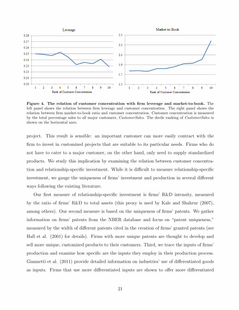
Figure 4. The relation of customer concentration with firm leverage and market-to-book. Theleft panel shows the relation between firm leverage and customer concentration. The right panel shows therelation between firm market-to-book ratio and customer concentration. Customer concentration is measuredby the total percentage sales to all major customers, CustomerSales. The decile ranking of CustomerSales isshown on the horizontal axes.

project. This result is sensible: an important customer can more easily contract with the

firm to invest in customized projects that are suitable to its particular needs. Firms who do

not have to cater to a major customer, on the other hand, only need to supply standardized

products. We study this implication by examining the relation between customer concentra-

tion and relationship-specific investment. While it is difficult to measure relationship-specific

investment, we gauge the uniqueness of firms’ investment and production in several different

ways following the existing literature.

Our first measure of relationship-specific investment is firms’ R&D intensity, measured

by the ratio of firms’ R&D to total assets (this proxy is used by Kale and Shahrur (2007),

among others). Our second measure is based on the uniqueness of firms’ patents. We gather

information on firms’ patents from the NBER database and focus on “patent uniqueness,”

measured by the width of different patents cited in the creation of firms’ granted patents (see

Hall et al. (2001) for details). Firms with more unique patents are thought to develop and

sell more unique, customized products to their customers. Third, we trace the inputs of firms’

production and examine how specific are the inputs they employ in their production process.

Giannetti et al. (2011) provide detailed information on industries’ use of differentiated goods

as inputs. Firms that use more differentiated inputs are shown to offer more differentiated

21

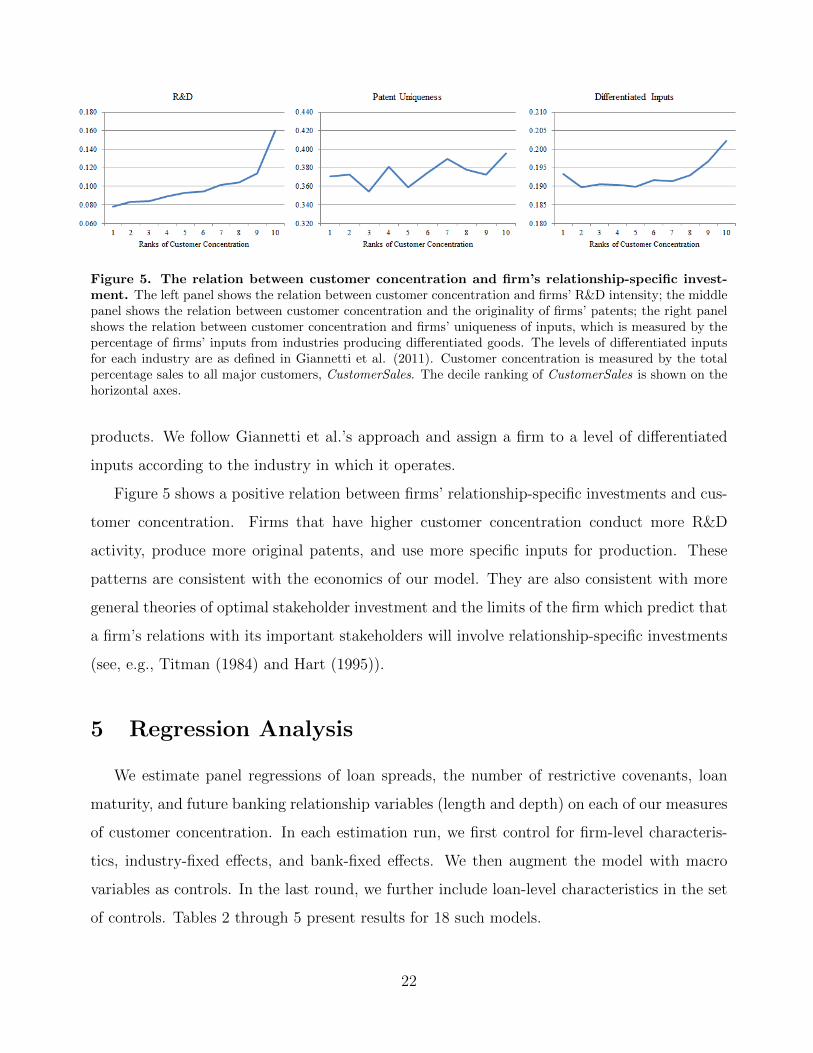
Figure 5. The relation between customer concentration and firm’s relationship-specific invest-ment. The left panel shows the relation between customer concentration and firms’ R&D intensity; the middlepanel shows the relation between customer concentration and the originality of firms’ patents; the right panelshows the relation between customer concentration and firms’ uniqueness of inputs, which is measured by thepercentage of firms’ inputs from industries producing differentiated goods. The levels of differentiated inputsfor each industry are as defined in Giannetti et al. (2011). Customer concentration is measured by the totalpercentage sales to all major customers, CustomerSales. The decile ranking of CustomerSales is shown on thehorizontal axes.

products. We follow Giannetti et al.’s approach and assign a firm to a level of differentiated

inputs according to the industry in which it operates.

Figure 5 shows a positive relation between firms’ relationship-specific investments and cus-

tomer concentration. Firms that have higher customer concentration conduct more R&D

activity, produce more original patents, and use more specific inputs for production. These

patterns are consistent with the economics of our model. They are also consistent with more

general theories of optimal stakeholder investment and the limits of the firm which predict that

a firm’s relations with its important stakeholders will involve relationship-specific investments

(see, e.g., Titman (1984) and Hart (1995)).

5 Regression Analysis

We estimate panel regressions of loan spreads, the number of restrictive covenants, loan

maturity, and future banking relationship variables (length and depth) on each of our measures

of customer concentration. In each estimation run, we first control for firm-level characteris-

tics, industry-fixed effects, and bank-fixed effects. We then augment the model with macro

variables as controls. In the last round, we further include loan-level characteristics in the set

of controls. Tables 2 through 5 present results for 18 such models.

22

Table 2 shows the results for regressions of loan spreads on measures of customer con-

centration, CustomerSales and CustomerSize. Both measures have significant and positive

loadings across all estimations, suggesting that firms with a higher customer concentration

face higher loan spreads on their next loan. The most conservative set of estimates in the table

(column (6), featuring the full set of controls) suggests that a one-standard-deviation increase

in customer concentration is associated with an 10 basis points increase in loan spread. This

amounts to a 6% increase relative to the average loan spread of 173 basis points. Our results

suggest that banks consider customer concentration as a negative factor affecting firms’ credit

quality; a factor that is consistently priced into loan mark-ups.

Table 2 About Here

Table 3 shows results for the number of restrictive covenants. Both measures of customer

concentration return positive and statistically significant loadings across all regressions, sug-

gesting that firms with high customer concentration tend to have more covenants written

in their new loan contracts. The estimates from column (6) indicate that a one-standard-

deviation increase in customer concentration is associated with a 0.2 increase in the number of

loan covenants, which accounts for a 12% increase relative to the average number of covenants

(1.8 covenants) for the loans in the sample.

Table 3 About Here

Table 4 shows the results for loan maturity. In this set of regressions, only term loans

are used, since revolvers indicate the option of borrowing, but do not indicate loan matu-

rity. Both measures of customer concentration attract negative coefficients suggesting that

firms with higher levels of customer concentration receive loans with shorter maturity. The

statistical significance of these estimates is more marginal. In economic terms, however, a

one-standard-deviation increase in customer concentration is associated a 2-month reduction

in loan maturity; compared to the sample average maturity of 45 months.

Table 4 About Here

23

We also study the impact of customer concentration on length and depth of the relationship

of the supplier firm and its bank. The results are reported in Table 5. The most conservative

estimates in the table suggest that a one-standard-deviation increase in customer concentration

is associated with 0.3 fewer loans in the future extended by the firm’s current bank; a 7% drop

relative to the sample mean. A one-standard-deviation increase in concentration is associated

with 0.4 fewer years of future relations with the bank; a 15% drop relative to the mean.

Table 5 About Here

These results are internally coherent and consistent with the predictions of our simple the-

oretical model. They show that a more concentrated customer base is associated with costlier,

stricter loan terms for the firm’s new loans, including higher interest rate spreads, more re-

strictive covenants, and shorter maturities. Customer concentration is also associated with the

deterioration of firm–bank associations, represented by shorter relations and fewer loans issued

by the bank in the future.

6 An Instrumental Variables Approach

Although common in the literature, estimations such as those performed in the previous

section are subject to concerns about estimation biases. In particular, concerns about uncon-

trolled heterogeneity that confounds the effects of customer concentration on loan terms may

arise from the fact the model lacks an explicit source of exogenous variation in concentration.

To allay those concerns, we perform tests that exploit shifts in the concentration of a firm’s

customer base; shifts whose cause are independent of firm borrowing terms.

We use aggregate merger and acquisition activity in customers’ industries (downstream

M&A) as an instrument in assessing the impact of customer concentration on firms’ loan terms

and banking relationships. Our instrumental approach implies that suppliers will face a more

concentrated customer base following M&A waves in their customers’ industries (inclusion re-

striction). We will verify that this is indeed the case in the tests below. The approach also

implies that downstream M&A affects suppliers’ borrowing terms through customer–supplier

links (exclusion restriction). Existing research shows that this is a plausible prior (e.g., Fee

24

and Thomas (2004) and Greene et al. (2013)). Downstream M&A activity is not a policy

variable of the supplier. Yet, downstream M&A activity (among customers) is shown to be

directly associated with higher bargaining power and higher trading profits against suppliers.

6.1 Measuring M&A Activity in the Customer Industry

We gather information on M&A deals from SDC database and apply the following data

filters following Ahern and Harford (2014): 1) only include completed deals, announced be-

tween 1986 and 2011; 2) both the acquirer and target are U.S. firms; 3) the acquirer can be

matched with a Compustat identifier; 4) the acquirer purchases at least 20% of the target

during the transaction, and owns more than 51% after the transaction; and 5) the acquirer

does not directly acquire its suppliers (exclude deals whose target reports the acquirer as a

customer during the 5-year window around the acquisition). Finally, we exclude suppliers who

are in the same 2-digit SIC industry as their customers.

We use the transaction values of M&As scaled by the acquirers’ total sales as a proxy

for acquisition activity. An industry-level 5-year mean acquisition activity is measured as the

average acquisition of firms in the industry over the past five years. Each of the firms in our

sample supplies products to a portfolio of customers, and those customers may be in different

industries. For each sample firm, we gauge the potential impact of downstream M&A activity

on customer concentration by taking the average of the 5-year acquisition activity across the

industries to which the firm’s customers belong. We refer to this variable as CustumerM&A.

6.2 IV Specification and Results

We use two-stage least square regressions to reassess the impact of customer concentration

on firm loan terms. In the first stage, we regress customer concentration measures (Custom-

erSales and CustomerSize) on CustumerM&A, together with a full set of controls. In the

second stage, we regress borrowing terms and banking relationship variables on the projected

customer concentration measures, together with controls. The two-stage system for borrowing

terms can be written as follows:

25

CustomerConcentrationi,k,t = β1 + β2CustomerM&Ai,t + Controls+ εi,k,t [First stage] (15a)

LoanTermsi,k,t = β3 + β4 ̂CustomerConcentrationi,k,t + Controls+ νi,k,t, [Second stage] (15b)

where i indicates the supplier, k indicates newly initiated loans, t indicates the fiscal year.

LoanTerms includes the loan term variables LoanSpread, LoanMaturity, and LoanCovenants.

CustomerConcentration indicates customer concentration measures. ̂CustomerConcentration

denotes the predicted value of customer concentration from the first-stage regression, reflecting

the variation of customer concentration induced by the variation M&A activity in customers’

industries. Controls contains the set of control variables used in our baseline regressions,

including firm-level controls, macro variables, loan-level controls, and bank-fixed effects.

Our IV tests further account for unobserved industry dynamics that can drive both down-

stream merger waves and firms’ credit terms. In particular, economic and technological shocks

to an industry can lead to merger waves (Harford (2005)). These industry-wide shocks can

further propagate along the supply chain and lead to merger waves in downstream industries

(Ahern and Harford (2014)). To control for these industry-level, time-varying dynamics that

may confound our results, we incorporate industry-year-fixed effects. The fixed effects ap-

proach removes any unobservable shock that is common to an industry in a given time period,

thus preventing it from contaminating the exclusion restriction of our instrument.

The two-stage regressions for banking relationships take a similar form:

CustomerConcentrationi,h,t = β1 + β2CustomerM&Ai,t + Controls+ εi,h,t [First stage] (16a)

BankingRelationi,h,t = β3 + β4 ̂CustomerConcentrationi,h,t + Controls+ ηi,h,t, [Second stage] (16b)

where h indicates the lending bank. BankingRelation is the measures for bank relationships:

FutureDuration and FutureLoans.

In the first stage (Eqs. (15a) and (16a)), we expect β2 to be positive, indicating that suppli-

ers experience increases in customer concentration following high levels of M&A activity in the

customers’ industries. In the second stage, we expect β4 to be positive for the loan spreads and

covenants regressions, and negative for the loan maturity and bank relationship regressions.

Table 6 shows the first-stage regression results for customer concentration on customer in-

dustry acquisition activity. The instrument loads significantly positively in all models. For

brevity of presentation, we only present the results for the customer concentration measure Cus-

26

tomerSales. The results are similar for CustomerSize. Results in Table 6 are consistent with the

prior of our identification strategy implying that firms face more concentrated customer bases

following high levels of M&A activity in their customers’ industries. In economic terms, a one-

standard-deviation increase in downstream M&A contributes to a 3.6 per cent increase in cus-

tomer concentration, which is an 11% increase relative to the average customer concentration.

Notably, the F -statistics from the first-stage regressions pass the weak identification tests at the

5% level. The Kleinberg-Paap statistics also pass the under-identification tests at the 5% level.

Table 6 About Here

Table 7 shows the second-stage regression results of loan terms and banking relationships on

the instrumented customer concentration. Consistent with our OLS results, the instrumented

customer concentration is positive and statistically significant in the loan spreads and loan

covenants regressions. They are negative and statistically significant in the loan maturity and

future banking relationship regressions.

Table 7 About Here

Our instrumental variables approach yields robust findings indicating that increases in cus-

tomer concentration lead to higher loan spreads and more loan covenants for supplier firms.

Higher customer concentration also leads to lower loan maturity, shorter banking relationships,

and fewer loans extended by the same bank in the future. In all, the evidence we gather suggests

that while customer concentration may make supply chain relations more efficient and increase

firm profits, a deeper exposure to a small set of customers also has negative consequences for

a firm’s relations with its creditors.

7 Customer Financial Condition

To better understand why customer concentration leads to worse credit terms, we look at

the types of customer characteristics that have an effect on loan terms. To do this, we study

the financial conditions of major customers. Wilner (2000) argues that suppliers tend to grant

27

more concessions to financially-distressed customers in order to maintain product market rela-

tionships. Accordingly, one would expect a firm whose customers are in worse financial shape

to receive worse loan terms, including higher spreads, more covenants, and shorter maturity.

7.1 Measuring Customer Financial Condition

We design two measures of customer financial conditions. One measure is simply based

on customers’ leverage; the other is based on customers’ probability of default, as predicted

by the KMV-Merton model (Merton (1974) and Bharath and Shumway (2008)). When a cus-

tomer has a higher level of indebtedness, it may have difficulty maintaining existing purchase

schedules or paying suppliers on time. These problems will be more relevant for suppliers when

that customer is large. Accordingly, we construct a measure of customer financial condition

that aggregates customers’ leverage for each supplier. CustomerLeverage is defined as:

CustomerLeveragei =

ni∑j=1

%Salesij × Leveragej,

where Leveragej is the leverage of customer j. Higher values of CustomerLeverage indicate

that the firm’s customers are more indebted.

Beyond assessing leverage, we directly gauge customers’ financial distress using their prob-

ability of default based on Merton’s (1974) model. We follow Bharath and Shumway (2008)

and employ a reduced form model to calculate customers’ probability of default (“distance-to-

default”). For each supplier, we measure the average default likelihood of its major customers

using its percentage sales to these customers and refer to this variable as CustomerDefault.

The variable is defined as follows:

CustomerDefaulti =

ni∑j=1

%Salesij × πj,

where πj is the predicted probability of default for customer j. Similar to CustomerLeverage,

higher values of CustomerDefault indicate that the firm faces a more financially-distressed

customer base. According to our model, this firm is likely to receive worse loan terms.

28

7.2 Results

We report the impact of customers’ finances on suppliers’ borrowing terms in Table 8, where

we estimate models that resemble those of our baseline tests.9 Columns (1) and (2) of Table 8

show the relation between loan spreads and customer financial measures CustomerLeverage and

CustomerDefault. Both measures attain significant, positive loadings, suggesting that firms

facing large, likely financially-distressed customers experience higher interest spreads on their

new loans. Columns (3) and (4) show the relation between the number of restrictive covenants

and customers’ financial condition. The results suggest that banks impose more restrictive

covenants for firms with more financially-troubled customers. Finally, despite the weaker

statistical significance, results in columns (5) and (6) suggest that firms with more distressed

customers are offered shorter maturities on their new loans. Notably, the economic magnitudes

associated with the coefficients in Table 8 implies that the negative effects of customer concen-

tration on loan terms are even larger than those of our baseline tests in Tables 2 through 4.

Table 8 About Here

The results of this section are important in confirming the logic behind our base findings.

A deeper relation with a small set of customers has negative consequences for a firm’s relations

with its creditors. And more so the more financially unhealthy those customers are. In the

next two sections we discuss how fears associated with exposure and contagion may explain

banks’ decision to offer suppliers worse credit terms when they sell their output to a smaller

set of customers.

8 Depicting the Contagion Effect: The Case of GM

It is important to concretely describe how financial distress of large customers can nega-

tively impact the suppliers. To do so, we study the bankruptcy case of a large, high profile

company: General Motors (GM). GM filed for Chapter 11 bankruptcy in the Manhattan New

York federal court on June 1, 2009. In this section we show how the GM bankruptcy led to a

9Results on the duration and depth of bank relations are omitted for brevity, but are readily available.

29

measurable wealth loss for its suppliers’ investors during the year of the bankruptcy filing.

To conduct this examination, we follow the procedure used in Hertzel et al. (2008). We

first identify the ‘‘distress event date’’ for the bankruptcy as the date when the shareholders of

GM lost the most equity value in the period leading up to the bankruptcy filing. For the GM

bankruptcy, the relevant distress event date is 10/9/2008.10 We compute the abnormal return

reaction of the suppliers of GM during the five trading days around the distress event date.

We define abnormal returns as the daily stock returns minus market index returns on the same

trading day. To be in the sample, firms need to report GM as a major customer during the

year of GM’s bankruptcy and have available equity return data around the event date.

Table 9 shows the abnormal returns in the 5-trading-day window around the GM bankruptcy

event. The first column reports the name of the suppliers; the second column reports the im-

portance of GM to the suppliers, measured by the percentage of total sales dedicated to GM;

the third column shows the post-event abnormal returns of the suppliers; the last column shows

the t-statistics of the post-event abnormal returns. On average, suppliers of GM experience an

abnormal return of –8.9% during the 5-trading-day window after the distress date. The signifi-

cance of event-period returns is tested relative to the returns in a 100-trading-day window prior

to the month of the distress event. Given the mean and standard deviation of the pre-event ab-

normal returns, we calculate the t-statistics by dividing the difference between the event-period

and pre-event returns by the adjusted standard deviation from pre-event window. The abnor-

mal returns during the distress event are, on average, 8.6% lower than the abnormal returns

during the 100-trading-day window that precedes the bankruptcy. Comparing such differences

with standard deviation of a 5-day abnormal return, we get an average t-statistic of –4.9.

Table 9 About Here

Table 9 shows a strong negative relation between the returns around GM’s bankruptcy

and the importance of GM as a customer. That association can be gauged from the simple

correlation coefficient of –0.4 (p-value of 1%) for the relation between firms’ percentage sales to

GM and distress-event stock returns. This relation can also be illustrated with a concrete case.

10On that day, Standard & Poor’s Ratings Services placed GM on downgrade watch. GM’s share pricesdropped 22%.

30

American Axle Manufacturing attributed 78% of its total sales to GM during 2009. That firm’s

stock price plummeted 30% in the five trading days following news about GM being absorbed

by the market. These dramatic equity losses suggest that the financial distress of important

customers has large, negative effects on suppliers’ value.

The negative influence of GM’s bankruptcy on its suppliers can also be gathered from CDS

spreads. Three of GM’s principal suppliers have actively traded CDS data around the event

date: Lear corp, Ryder System inc, and TRW Automotive corp. Examining daily spreads

from 5-year CDS contracts we find that their CDS spreads increased significantly during the

5-trading-day window around GM’s distress event date.11 Table 10 shows the changes of CDS

spreads for these suppliers from a 10-trading-day pre-event window ((–12, –3) trading days prior

to 10/9/2008) to the 5-trading-day post-event window. The CDS spread of Lear increased from

1,314 to 2,154 basis points; a 64% hike. The CDS spread of TRW also increase dramatically

around GM bankruptcy; it nearly doubled, going from 742 to 1,386 basis points. Spreads on

Ryder’s CDSs also increased around that same event; from 165 to 208 basis points. The average

increase in CDS spreads across these suppliers to GM is 59% over their pre-bankruptcy spread.

All combined, this illustrative evidence suggests that the financial distress of GM imposes large

increases of credit risk to its suppliers, which became a natural concern for their lenders.

Table 10 About Here

The GM bankruptcy illustrates why lenders should be concerned with their borrowers are

exposed to large, distressed customers. We study this economic connection more systematically

in the next section.

9 Loan Failure

To substantiate our argument that firms with higher customer concentration face more

adverse credit terms because of deteriorated creditworthiness, we directly examine the rela-

tionship between supplier loan failure rate and customer concentration. Loan failures are costly

11We gather CDS data from Credit Market Analysis and Thomson Reuters.

31

for banks, especially when the loans are unsecured (Berger and Udell (1990)).12 Commercial

banks, in particular, are highly regulated intermediaries and the exposure to loan risk bears

tremendous costs for them. If customer concentration increases the likelihood of loan failure, it

should naturally lead to stricter loan terms and higher borrowing cost imposed by the banks.

We match our customer and loan datasets with the LoPucki database to test this idea.

Recall, the variable LoanFailure indicates whether the company files for bankruptcy before the

loan matures. To examine the conjecture that a more concentrated customer base is associated

with higher likelihood of supplier loan failure, we estimate the following logit regression model:

LoanFailurei,k,t = β0 +β1CustomerConcentrationi,t+β2FirmCharacteri,t+β3MacroV art

+ β4LoanCharacterk,t +∑g

Industryg +∑h

Bankh + εi,k,t, (17)

where CustomerConcentration includes CustomerSales, CustomerSize, CustomerLeverage, and

CustomerDefault. The models feature the same sets of controls used in our baseline regressions.

Table 11 reports results for CustomerSales and CustomerSize. Both customer concentration

variables have positive and significant loadings, suggesting that firms with more concentrated

customer base are more likely to fail during the existence of a loan contract, exposing their

banks to higher risk. To help interpret our estimates, note that the coefficient for Customer-

Size in column (8) suggests that a one-standard-deviation increase in customer concentration

is associated with a 2 per cent increase in loan failure rates. This is a sizable effect, especially

in comparison to the average loan failure rate of 6.5 per cent. In unreported tables, we further

show that firms are more likely to fail on their loans as their customers’ financial condition

deteriorates (proxied by CustomerLeverage and CustomerDefault).

Table 11 About Here

The results of this section show direct evidence that customer concentration is negatively

associated with firms’ credit quality. Specifically, firms with more concentrated customer bases

and selling to larger, financially-distressed customers are more likely to default on their loans.

12In our sample, only 57% of the loans are secured.

32

Consistent with our prior results, the higher loan failure rates help explain why lenders impose

costlier, stricter terms on loans offered to suppliers with these customer-base profiles, even

though these suppliers themselves are more profitable.

10 Concluding Remarks

Recent literature shows that customer concentration can increase firms’ operational effi-

ciency, leading to significant increases in profitability. While recognizing those gains, we exam-

ine the potential costs associated with deeper relationships between customers and suppliers.

Our study looks at how credit markets respond to customer-base concentration. It does

so by examining the credit terms offered by banks. Using detailed information on bank loans,

we study how customer-base concentration affects a firm’s borrowing terms, including loan

interest spread, maturity, and the number of restrictive covenants. We further gauge the im-

pact of customer profile on the length and intensity of suppliers’ relations with their banks.

Our tests show that higher levels of customer concentration increase the interest rates and the

number of restrictive covenants on a firm’s bank loans. Customer concentration also reduces

loan maturities and the duration and depth of banking relationships.

Exploring the cross-sectional variation in customer characteristics, we further show that

when firms have larger and more financially-distressed customers, they face even worse loan

terms. We also show direct evidence that a more concentrated customer base affects a firm’s

credit risk. In particular, suppliers with higher customer concentration and more financially-

troubled, large customers are more likely to default on their loans. This result corroborates our

argument that while customer concentration may make supply chain relations more efficient

and profitable, a deeper exposure to a small set of customers has negative consequences for

the firm’s relations with its creditors.

Understanding the various trade-offs associated with customer concentration is important,

since the modern business-to-business economy experiences increasing levels of customer con-

centration. Integration along the supply chain is fraught with incomplete contract problems

between customers and suppliers. These problems allow powerful customers to set trade terms

to their own advantage, while leaving suppliers “held-up” due to costly, relationship-specific

33

investments they may be forced to make. Our paper sheds light on one additional cost induced

by this incomplete contract friction. In particular, we show that hold-up problems can lead

to deterioration of suppliers’ credit quality. This phenomenon is reflected in the increased

borrowing costs and tightened debt contract terms required by banks. Future research would

benefit from understanding how bank contracting can complement or substitute for supplier

chain contracting. Overall, our analyses suggest that the cost related to customer concentra-

tion deserves better understanding and may give new insights into important research topics,

such as the limits of the modern corporation.

34

References

Ahern, K., Harford, J., 2014. “The importance of industry links in merger waves.” Journalof Finance forthcoming.

Banerjee, S., Dasgupta, S., Kim, Y., 2008. “Buyer-supplier relationships and the stakeholdertheory of capital structure.” Journal of Finance 63, 2507-2552.

Barrot, J. N., 2014. “Trade credit and industry dynamics: Evidence from trucking firms.”Working Paper.

Berger, A. N., Udell, G. F., 1990. “Collateral, loan quality and bank risk.” Journal ofMonetary Economics 25, 21-42.

Bharath, S., Shumway, T., 2008. “Forecasting default with the Merton distance to defaultmodel. ” Review of Financial Studies 21, 1339-1369.

Biais, B., Gollier, C., 1997. “Trade credit and credit rationing.” Review of Financial Studies10, 903-937.

Bolton, P., Scharfstein, D., 1998. “Corporate finance, the theory of the firm, and organiza-tions.” Journal of Economic Perspectives 12, 95-114.

Burkart, M., Ellingsen, T., 2004. “In-kind finance: A theory of trade credit.” Journal ofEconomic Perspectives 94, 569-590.

Campello, M., Lin, C., Ma, Y., Zou, H., 2011. “The real and financial implications ofcorporate hedging.” Journal of Finance 66, 1615-1647.

Cen, L., Dasgupta, S., Elkamhi, R., Pungaliya, R., 2014. “Reputation and loan contractterms: The role of principal customers.” Working Paper.

Chava, S., Roberts, M. R., 2008. “How does financing impact investment? The role of debtcovenants.” Journal of Finance 63, 2085-2121.

Cohen, L., Frazzini, A., 2008. “Economic links and predictable returns.” Journal of Finance63, 1977-2011.

Erel, I., Jang, Y., Weisbach, M. S., 2014. “Do acquisitions relieve target firms’ financialconstraints?” Journal of Finance forthcoming.

Fee, E., Thomas, S., 2004. “Sources of gains in horizontal mergers: Evidence from customer,supplier, and rival firms.” Journal of Financial Economics 74, 423-460.

Giannetti, M., Burkart, M., Elingsen, T., 2011. “What you sell is what you lend? Explainingtrade credit contracts.” Review of Financial Studies 24, 1261-1298.

Graham, J. R., Li, S., Qiu, J., 2008. “Corporate misreporting and bank loan contracting.”Journal of Financial Economics 89, 44-61.

Greene, D., Kini, O., Shenoy, J., 2013. “Buyer power in conglomerate acquisitions.” WorkingPaper.

Hall, B., Jaffe, A., Trajtenberg, M., 2001. “The NBER patent citations data file: Lessons,insights and methodological tools.” Working Paper.

35

Harford, J., 2005. “What drives merger waves?” Journal of Financial Economics 77, 529-560.

Hart, O., 1995. “Firms, contracts, and financial structure.” Oxford University Press.

Hennessy, C., Livdan, D., 2009. “Debt, bargaining, and credibility in firm supplier relation-ships.” Journal of Financial Economics 93, 382-399.

Hertzel, M. G., Li, Z., Officer, M. S., Rodgers, K. J., 2008. “Inter-firm linkages and the wealtheffects of financial distress along the supply chain.” Journal of Financial Economics 87,374-387.

Hertzel, M. G., Officer, M. S., 2012. “Industry contagion in loan spreads.” Journal of Finan-cial Economics 103, 493-506.

Irvine, P. J., Park, S. S., Yildizhan, C., 2013. “Customer-base concentration, profitabilityand distress across the corporate life cycle.” Working Paper.

Kale, J., Shahrur, H., 2007. “Corporate capital structure and the characteristics of suppliersand customers.” Journal of Financial Economics 83, 321-365.

Kelly, B., Lustig, H., Van Nieuwerburgh, S., 2013. “Firm volatility in granular networks.”Chicago Booth Research Paper.

Klein, B., Crawford, R., Alchian, A., 1978. “Vertical integration, appropriable rents, and thecompetitive contracting process.” Journal of Law and Economics 21, 297-326.

Kolay, M., Lemmon, M., Tashjian, E., 2012. “Spillover effects in the supply chain: Evidencefrom Chapter 11 filings.” Working Paper.

Lin, C., Ma, Y., Malatesta, P., Xuan, Y., 2011. “Ownership structure and the cost ofcorporate borrowing.” Journal of Financial Economics 100, 1-23.

Merton, R., 1974. “On the pricing of corporate debt: The risk structure of interest rates.”Journal of Finance 29, 449-470.

Murfin, J., Njoroge, K., 2013. “The implicit costs of trade credit borrowing by large firms.”Working Paper.

Patatoukas, P. N., 2012. “Customer-base concentration: Implications for firm performanceand capital markets.” The Accounting Review 87, 363-392.

Roberts, M. R., Sufi, A., 2009. “Renegotiation of financial contracts: Evidence from privatecredit agreements.” Journal of Financial Economics 93, 159-184.

Titman, S., Wessels, R., 1988. “The determinants of capital structure choice.” Journal ofFinance 43, 1-19.

Valta, P., 2012. “Competition and the cost of debt.” Journal of Financial Economics 105,661-682.

Wilner, B. S., 2000. “The exploitation of relationships in financial distress: The case of tradecredit.” Journal of Finance 55, 153-178.

36

Appendix A Variable Definitions

LoanSpread : All-in-Drawn loan spread over LIBOR

LoanCovenants : Total number of covenants on the loan package

LoanMaturity : Loan maturity in months

CustomerSales : Total percentage sales to all major customers

CustomerSize: Total size of all major customers, weighted by the firm’s percentage sales to

customer

CustomerLeverage: Leverage of major customers, weighted by the firm’s percentage sales to

customer

CustomerDefault : Probability of default of major customers predicted by Merton’s distance-

to-default model, weighted by the firm’s percentage sales to customer

Size: Log of total assets (AT)

Age: Years after a firm’s first appearance in Compustat database

Profitability : Operating income (OIBDP)/total assets

Tangibility : Property, plant, and equipment (PPENT)/total assets

M/B : (Stock price (PRCC)×shares outstanding (CSHO) + total assets – book equity (CEQ))/total

assets

Leverage: (Long-term debt (DLTT) + current debt (DLC))/total assets

Ratings : A dummy variable that equals 1 if the firm has a bond rating, 0 otherwise

CreditSpread : Yield spread between average AAA-rated corporate bonds and average BBB-

rated corporate bonds

TermSpread : Yield spread between 10-year Treasury bond and 3-month Treasury bills

GDPGrowth: Quarterly average of GDP growth rate of the year

LoanSize: Log of total loan amount (in dollars)

LoanType: A dummy variable that equals 1 if the loan is a term loan, 0 if loan is a revolver

37

Appendix B

Proof for ∂R∂λ< 0:

The interest rate R offered by the bank is a function of both λ and the average quality of

firms that choose project A. Therefore,

∂R

∂λ=dR

dλ+

∂R

∂E[p|p > p∗]

dE[p|p > p∗]

λ. (18)

The first term is the direct effect of λ on R, which is apparently negative (since ηE[p|p >p∗]α(1 − µ) < 1). This results from the fact that when the major customer is healthy, the

supplier is more likely to get paid in full, and will be less likely to default on its bank loan. The

second term is the indirect effect of λ on R, through its effect on the equilibrium threshold p∗.

It is easy to see that ∂R∂E[p|p>p∗] is negative, since when the firms conducting the risky project

are of better quality on average, the bank faces less default. dE[p|p>p∗]dλ

has the same sign as dp∗

dλ,

since the higher the threshold, the higher quality the average firms are above the threshold.

Eq. (11) can be simplified to:

p∗ =β

αµVA+

βαµVA

D + C

αµVA/λ−D(19)

where D = R − α(1 − µ) > 0 since R > 1 and α(1 − µ) < 1; and C = βµ(VB − 1) > 0. It

follows that dp∗

dλ> 0, dE[p|p>p∗]

dλ> 0, and that ∂R

∂λ< 0.

38

Table 1Summary StatisticsThis table shows the summary statistics of the firm characteristics variables, customer variables, and loanterm variables. The sample spans the 1985–2010 window, featuring manufacturing firms (SIC 2000–3999) inCompustat that have available firm characteristics and loan term variables. All continuous variables exceptleverage and the number of covenants (count) are winsorized within 5 and 95 percentile. Leverage is restrictedto the 0–1 range.

Variables Mean Std. Dev. p25 p50 p75 #Obs

LoanSpread 173.16 106.28 75 160 250 2983

LoanMaturity 45 22 25 48 60 2983

LoanCovenants 1.80 1.65 0 2 3 2983

FutureLoans 4.23 4.05 2 3 5 1242

FutureDuration 2.90 3.77 0 2 4 2055

CustomerSales 0.3 0.2 0.15 0.23 0.39 2983

CustomerSize 2.72 1.86 1.29 2.05 3.48 2903

CustomerLeverage 0.09 0.08 0.03 0.06 0.11 2903

CustomerDefault 0.04 0.07 0.00 0.01 0.06 2456

Size 6.38 1.62 5.13 6.41 7.61 2983

Age 18.41 16.45 5 12 31 2983

Profitability 0.12 0.11 0.08 0.13 0.18 2983

Tangibility 0.26 0.15 0.15 0.24 0.37 2983

M/B 1.71 1.06 1.12 1.38 1.91 2983

Leverage 0.33 0.21 0.18 0.31 0.45 2983

Ratings 0.48 0.5 0 0 1 2983

LoanType 0.28 0.45 0 0 1 2983

39

Table 2Loan Spreads and Customer ConcentrationThis table shows the relation between loan spreads and customer concentration. The dependent variable is All-in-Drawn loan spread (LoanSpread). All regressions use industry-fixed effects and bank-fixed effects. Industryis classified as 2-digit SIC industry and the lending banks are classified by their ultimate parents. Standarderrors are clustered by industry. Robust t-statistics are shown in parentheses. Columns (1) through (3) showthe regression results for CustomerSales: the sum of the percentage sales to the set of customers a firm reportsas “major customers”. Columns (4) through (6) show the regression results for CustomerSize: the total sizeof all major customers, weighted by the firm’s percentage sales to these customers.

Dep. Var.: LoanCovenants CustomerConcentration is CustomerSales CustomerConcentration is CustomerSize

(1) (2) (3) (4) (5) (6)

CustomerConcentration 52.56*** 47.14** 40.89*** 7.05*** 5.90** 5.28***(3.15) (2.67) (3.32) (3.78) (2.84) (3.72)

Size -27.58*** -28.28*** -17.69*** -28.11*** -28.64*** -17.97***(-10.44) (-9.60) (-5.40) (-10.36) (-9.99) (-5.43)

Age -0.78*** -0.96*** -0.60*** -0.80*** -0.98*** -0.61***(-3.07) (-4.30) (-2.88) (-3.29) (-4.56) (-3.07)

Profitability -272.89*** -260.23*** -246.94*** -292.40*** -284.38*** -273.44***(-3.20) (-3.62) (-3.89) (-3.53) (-4.12) (-4.23)

Tangibility -20.65 -4.89 -27.66 -16.13 -1.90 -22.23(-0.79) (-0.24) (-0.77) (-0.63) (-0.09) (-0.62)

M/B -11.07*** -6.58* -3.75 -9.23** -4.60 -1.83(-3.09) (-1.88) (-0.90) (-2.20) (-1.07) (-0.40)

Leverage 135.13*** 146.97*** 128.86*** 138.60*** 149.30*** 131.47***(7.92) (10.58) (8.49) (7.53) (10.01) (8.21)

Ratings 38.08*** 37.98*** 35.74*** 37.94*** 38.06*** 35.24***(5.60) (5.80) (4.68) (5.55) (5.83) (4.62)

CreditSpread 87.21*** 81.53*** 82.11*** 76.32***(5.37) (5.49) (5.17) (4.97)

TermSpread 1.74 3.40 2.98 4.42*(0.75) (1.31) (1.33) (1.69)

GDPGrowth -3.96 -4.79* -4.18 -5.18**(-1.47) (-1.96) (-1.60) (-2.08)

LoanMaturity 5.91 6.48(1.50) (1.61)

LoanSize -15.77*** -16.02***(-5.66) (-5.69)

LoanType 45.78*** 44.87***(6.86) (6.76)

Observations 3,045 3,045 2,983 2,965 2,965 2,903R-squared 0.45 0.52 0.61 0.45 0.52 0.62

Robust t-statistics in parentheses*** p-value<0.01, ** p-value<0.05, * p-value<0.10

40

Table 3Number of Covenants and Customer ConcentrationThis table shows the relation between the number of covenants written on bank loans and customer con-centration. The dependent variable is the number of loan covenants (LoanCovenants). All regressions useindustry-fixed effects and bank-fixed effects. Industry is classified as 2-digit SIC industry and the lendingbanks are classified by their ultimate parents. Standard errors are clustered by industry. Robust t-statisticsare shown in parentheses. Columns (1) through (3) show the regression results for CustomerSales. Columns(4) through (6) show the regression results for CustomerSize.

Dep. Var.: LoanCovenants CustomerConcentration is CustomerSales CustomerConcentration is CustomerSize

(1) (2) (3) (4) (5) (6)

CustomerConcentration 1.04*** 1.01*** 0.95*** 0.12*** 0.11*** 0.09***

(4.85) (4.81) (2.75) (4.98) (4.89) (3.31)

Size -0.24*** -0.23*** -0.22*** -0.24*** -0.24*** -0.18***

(-4.20) (-4.38) (-4.08) (-4.17) (-4.35) (-6.31)

Age -0.00 -0.00 0.00 -0.00 -0.00 0.01**

(-1.02) (-1.20) (1.13) (-1.14) (-1.31) (2.58)

Profitability 0.79 0.83 1.59*** 0.66 0.73 1.57**

(1.15) (1.28) (3.24) (1.07) (1.18) (2.54)

Tangibility -0.53 -0.39 -0.45 -0.58 -0.46 -0.18

(-1.11) (-0.82) (-0.71) (-1.15) (-0.94) (-0.37)

M/B -0.15*** -0.13*** -0.06* -0.13** -0.12** -0.04

(-3.04) (-3.06) (-1.66) (-2.41) (-2.59) (-0.72)

Leverage 0.73** 0.72** -0.20 0.74** 0.73** -0.17

(2.47) (2.70) (-0.79) (2.66) (2.84) (-0.88)

Ratings 0.20** 0.19** 0.16 0.20** 0.19** 0.08

(2.32) (2.18) (1.37) (2.23) (2.14) (1.09)

CreditSpread 1.46*** 1.01*** 1.38*** 1.05***

(4.03) (4.09) (3.89) (3.55)

TermSpread -0.11* -0.11* -0.10* -0.11*

(-1.90) (-1.86) (-1.75) (-2.06)

GDPGrowth 0.21*** 0.23*** 0.21*** 0.23***

(4.56) (5.25) (4.76) (5.38)

LoanSpread 0.68*** 0.71***

(11.81) (25.99)

LoanMaturity 0.21*** 0.27***

(3.82) (5.49)

LoanSize 0.13*** 0.12**

(3.54) (2.17)

LoanType 0.06 0.06

(1.52) (1.28)

Observations 3,055 3,055 2,983 2,975 2,975 2,903

R-squared 0.17 0.19 0.33 0.17 0.19 0.28

Robust t-statistics in parentheses

*** p-value<0.01, ** p-value<0.05, * p-value<0.10

41

Table 4Loan Maturity and Customer ConcentrationThis table shows the relation between the bank loan maturity (in months) and customer concentration. Thedependent variable is loan maturity (LoanMaturity). Only term loans are considered for this test. Allregressions use industry-fixed effects and bank-fixed effects. Industry is classified as 2-digit SIC industry andthe lending banks are classified by their ultimate parents. Standard errors are clustered by industry. Robustt-statistics are shown in parentheses. Columns (1) through (3) show the regression results for CustomerSales.Columns (4) through (6) show the regression results for CustomerSize.

Dep. Var.: LoanMaturity CustomerConcentration is CustomerSales CustomerConcentration is CustomerSize

(1) (2) (3) (4) (5) (6)

CustomerConcentration -5.83* -5.70* -8.33** -0.77 -0.68 -1.04**

(-1.83) (-2.03) (-2.27) (-1.71) (-1.71) (-2.12)

Size -0.33 -0.28 -2.30 -0.38 -0.34 -2.35

(-0.26) (-0.22) (-1.73) (-0.29) (-0.25) (-1.74)

Age -0.24*** -0.20** -0.16*** -0.23** -0.19** -0.14***

(-3.16) (-2.86) (-3.10) (-2.91) (-2.61) (-2.93)

Profitability 44.20*** 45.07*** 49.95*** 42.79*** 44.72*** 49.80***

(4.63) (4.27) (4.40) (4.05) (3.90) (4.06)

Tangibility -18.46** -18.27** -19.26** -18.61** -18.24** -19.82**

(-2.44) (-2.48) (-2.61) (-2.37) (-2.37) (-2.57)

M/B -2.29 -2.91* -3.19** -2.49* -3.17** -3.43**

(-1.61) (-2.01) (-2.34) (-1.76) (-2.23) (-2.53)

Leverage 12.07 9.95 4.04 12.40 10.46 4.07

(1.68) (1.38) (0.55) (1.60) (1.34) (0.52)

Ratings 5.09 4.50 2.78 4.79 4.14 2.20

(1.57) (1.43) (0.90) (1.49) (1.30) (0.75)

CreditSpread -2.63 -5.57 -1.77 -4.75

(-0.49) (-0.94) (-0.31) (-0.76)

TermSpread -1.40 -0.91 -1.59* -1.10

(-1.71) (-1.17) (-1.85) (-1.37)

GDPGrowth 2.06** 2.26** 2.14** 2.38**

(2.21) (2.46) (2.22) (2.55)

LoanSpread 4.01 4.70**

(1.74) (2.28)

LoanSize 4.25*** 4.49***

(3.21) (3.43)

Observations 903 903 894 879 879 870

R-squared 0.23 0.27 0.29 0.23 0.27 0.30



42

Table 5Future Bank Relations and Customer ConcentrationThis table shows the relation between future bank relationships to a firm and the firm’s customer concentration.The dependent variable is future bank relationships, as measured by the number of loans extended by the samebank (FutureLoans) and the duration of banking relationships in the future (FutureDuration). All regressionsuse industry-fixed effects and bank-fixed effects. Industry is classified as 2-digit SIC industry and lendingbanks are classified by their ultimate parents. Standard errors are clustered by industry. Robust t-statisticsare shown in parentheses. Columns (1) and (2) show the regression results for CustomerSales. Columns (3)and (4) show the regression results for CustomerSize.

CustomerConcentration is CustomerSales CustomerConcentration is CustomerSize

(1) (2) (3) (4)

Dep. Var.: FutureLoans FutureDuration FutureLoans FutureDuration

CustomerConcentration -1.08 -1.99*** -0.16* -0.24***

(-1.65) (-4.23) (-1.96) (-4.39)

Size 0.17 0.16 0.15 0.15

(0.64) (1.05) (0.54) (0.97)

Age -0.03** -0.02*** -0.03** -0.01**

(-2.69) (-2.92) (-2.47) (-2.74)

Profitability 2.64 5.90*** 2.44 5.91***

(1.06) (5.34) (0.93) (5.11)

Tangibility 2.33* 2.20*** 2.50* 2.23***

(1.75) (3.79) (1.76) (3.71)

M/B 0.26 0.08 0.24 0.06

(1.18) (0.67) (1.07) (0.51)

Leverage 1.11 0.14 0.97 0.09

(1.48) (0.29) (1.28) (0.18)

Ratings 0.96** 0.92** 0.98** 0.95***

(2.23) (2.84) (2.22) (2.89)

CreditSpread -1.03 -1.84* -0.97 -1.64

(-1.42) (-2.03) (-1.27) (-1.72)

TermSpread 0.11 0.39*** 0.13 0.37***

(1.22) (4.83) (1.32) (4.56)

GDPGrowth 0.03 -0.02 0.04 -0.01

(0.39) (-0.22) (0.48) (-0.13)

Observations 1,242 2,055 1,210 1,996

R-squared 0.18 0.20 0.18 0.20



43

Table 6First-Stage Results for IV EstimationsThis table shows the first-stage regression results of a firm’s customer concentration on the average customers’industry acquisition activity (CustomerM&A). The dependent variable is customer concentration, measuredby CustomerSales. All regressions use industry-year-fixed effects and bank-fixed effects. Standard errors areclustered by industry. Robust t-statistics are shown in parentheses.

(1) (2) (3) (4) (5)Dep. Var. in the Second Stage LoanSpread LoanCovenants LoanMaturity FutureDuration FutureLoans

CustomerM&A 5.82*** 5.63*** 6.61*** 5.51*** 5.51***(3.62) (3.61) (3.04) (3.81) (3.81)

Size -0.01 -0.01 -0.01 -0.02 -0.02(-0.97) (-0.68) (-0.37) (-1.28) (-1.28)

Age -0.00* -0.00 -0.00 -0.00** -0.00**(-1.77) (-1.60) (-1.19) (-2.34) (-2.34)

Profitability 0.06 0.09 0.04 -0.02 -0.02(1.08) (1.53) (0.21) (-0.22) (-0.22)

Tangibility -0.05 -0.04 -0.08 0.04 0.04(-0.54) (-0.45) (-0.73) (0.49) (0.49)

M/B -0.01 -0.01 -0.01 -0.02 -0.02(-1.71) (-1.54) (-0.38) (-1.42) (-1.42)

Leverage -0.07*** -0.09*** -0.15* -0.10*** -0.10***(-3.78) (-3.36) (-2.07) (-5.95) (-5.95)

Ratings 0.01 0.01 0.02 0.04* 0.04*(0.39) (0.27) (0.46) (1.86) (1.86)

LoanSpread 0.02 0.03(1.28) (1.10)

LoanMaturity 0.01 0.01(0.99) (0.78)

LoanSize 0.01 0.01 0.01(1.05) (1.52) (0.36)

LoanType -0.01 -0.01(-0.94) (-1.70)

Observations 1,957 1,957 570 1,364 1,364R-squared 0.40 0.40 0.59 0.21 0.21

First Stage F-test 13.09 13.05 9.25 10.03 10.03p-value 0.00 0.00 0.01 0.01 0.01Kleibergen-Paap LM Stat 5.97 5.67 6.7 4.66 4.66p-value 0.01 0.02 0.01 0.04 0.04


44

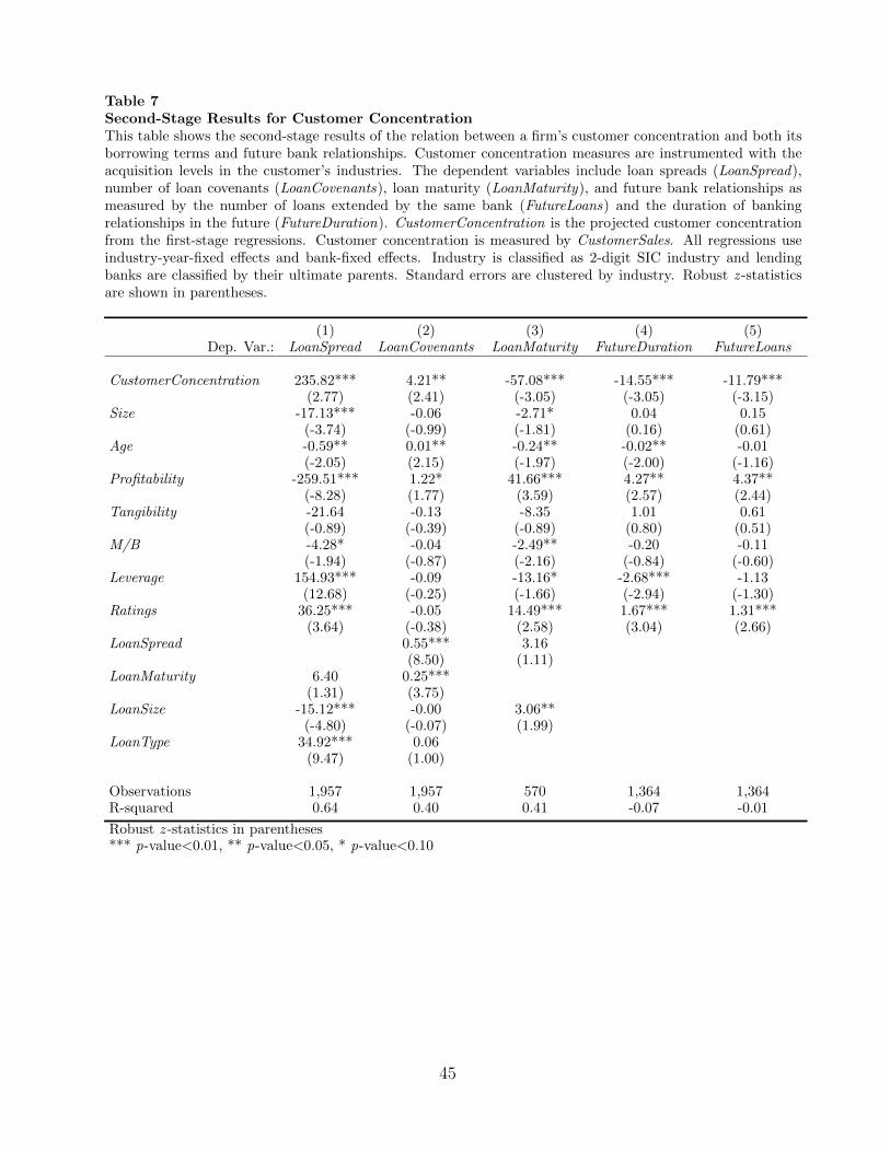
Table 7Second-Stage Results for Customer ConcentrationThis table shows the second-stage results of the relation between a firm’s customer concentration and both itsborrowing terms and future bank relationships. Customer concentration measures are instrumented with theacquisition levels in the customer’s industries. The dependent variables include loan spreads (LoanSpread),number of loan covenants (LoanCovenants), loan maturity (LoanMaturity), and future bank relationships asmeasured by the number of loans extended by the same bank (FutureLoans) and the duration of bankingrelationships in the future (FutureDuration). CustomerConcentration is the projected customer concentrationfrom the first-stage regressions. Customer concentration is measured by CustomerSales. All regressions useindustry-year-fixed effects and bank-fixed effects. Industry is classified as 2-digit SIC industry and lendingbanks are classified by their ultimate parents. Standard errors are clustered by industry. Robust z -statisticsare shown in parentheses.

(1) (2) (3) (4) (5)Dep. Var.: LoanSpread LoanCovenants LoanMaturity FutureDuration FutureLoans

CustomerConcentration 235.82*** 4.21** -57.08*** -14.55*** -11.79***(2.77) (2.41) (-3.05) (-3.05) (-3.15)

Size -17.13*** -0.06 -2.71* 0.04 0.15(-3.74) (-0.99) (-1.81) (0.16) (0.61)

Age -0.59** 0.01** -0.24** -0.02** -0.01(-2.05) (2.15) (-1.97) (-2.00) (-1.16)

Profitability -259.51*** 1.22* 41.66*** 4.27** 4.37**(-8.28) (1.77) (3.59) (2.57) (2.44)

Tangibility -21.64 -0.13 -8.35 1.01 0.61(-0.89) (-0.39) (-0.89) (0.80) (0.51)

M/B -4.28* -0.04 -2.49** -0.20 -0.11(-1.94) (-0.87) (-2.16) (-0.84) (-0.60)

Leverage 154.93*** -0.09 -13.16* -2.68*** -1.13(12.68) (-0.25) (-1.66) (-2.94) (-1.30)

Ratings 36.25*** -0.05 14.49*** 1.67*** 1.31***(3.64) (-0.38) (2.58) (3.04) (2.66)

LoanSpread 0.55*** 3.16(8.50) (1.11)

LoanMaturity 6.40 0.25***(1.31) (3.75)

LoanSize -15.12*** -0.00 3.06**(-4.80) (-0.07) (1.99)

LoanType 34.92*** 0.06(9.47) (1.00)

Observations 1,957 1,957 570 1,364 1,364R-squared 0.64 0.40 0.41 -0.07 -0.01

Robust z -statistics in parentheses*** p-value<0.01, ** p-value<0.05, * p-value<0.10

45

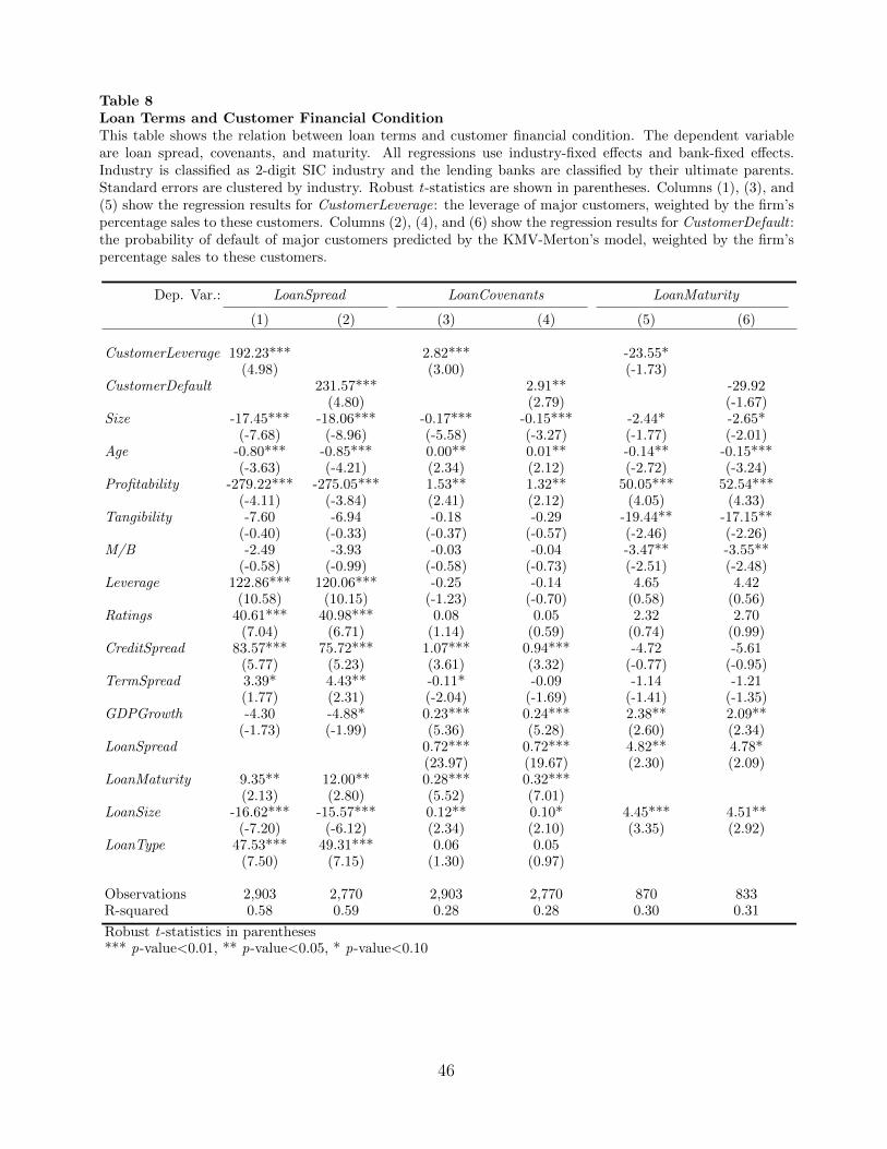
Table 8Loan Terms and Customer Financial ConditionThis table shows the relation between loan terms and customer financial condition. The dependent variableare loan spread, covenants, and maturity. All regressions use industry-fixed effects and bank-fixed effects.Industry is classified as 2-digit SIC industry and the lending banks are classified by their ultimate parents.Standard errors are clustered by industry. Robust t-statistics are shown in parentheses. Columns (1), (3), and(5) show the regression results for CustomerLeverage: the leverage of major customers, weighted by the firm’spercentage sales to these customers. Columns (2), (4), and (6) show the regression results for CustomerDefault :the probability of default of major customers predicted by the KMV-Merton’s model, weighted by the firm’spercentage sales to these customers.

Dep. Var.: LoanSpread LoanCovenants LoanMaturity

(1) (2) (3) (4) (5) (6)

CustomerLeverage 192.23*** 2.82*** -23.55*(4.98) (3.00) (-1.73)

CustomerDefault 231.57*** 2.91** -29.92(4.80) (2.79) (-1.67)

Size -17.45*** -18.06*** -0.17*** -0.15*** -2.44* -2.65*(-7.68) (-8.96) (-5.58) (-3.27) (-1.77) (-2.01)

Age -0.80*** -0.85*** 0.00** 0.01** -0.14** -0.15***(-3.63) (-4.21) (2.34) (2.12) (-2.72) (-3.24)

Profitability -279.22*** -275.05*** 1.53** 1.32** 50.05*** 52.54***(-4.11) (-3.84) (2.41) (2.12) (4.05) (4.33)

Tangibility -7.60 -6.94 -0.18 -0.29 -19.44** -17.15**(-0.40) (-0.33) (-0.37) (-0.57) (-2.46) (-2.26)

M/B -2.49 -3.93 -0.03 -0.04 -3.47** -3.55**(-0.58) (-0.99) (-0.58) (-0.73) (-2.51) (-2.48)

Leverage 122.86*** 120.06*** -0.25 -0.14 4.65 4.42(10.58) (10.15) (-1.23) (-0.70) (0.58) (0.56)

Ratings 40.61*** 40.98*** 0.08 0.05 2.32 2.70(7.04) (6.71) (1.14) (0.59) (0.74) (0.99)

CreditSpread 83.57*** 75.72*** 1.07*** 0.94*** -4.72 -5.61(5.77) (5.23) (3.61) (3.32) (-0.77) (-0.95)

TermSpread 3.39* 4.43** -0.11* -0.09 -1.14 -1.21(1.77) (2.31) (-2.04) (-1.69) (-1.41) (-1.35)

GDPGrowth -4.30 -4.88* 0.23*** 0.24*** 2.38** 2.09**(-1.73) (-1.99) (5.36) (5.28) (2.60) (2.34)

LoanSpread 0.72*** 0.72*** 4.82** 4.78*(23.97) (19.67) (2.30) (2.09)

LoanMaturity 9.35** 12.00** 0.28*** 0.32***(2.13) (2.80) (5.52) (7.01)

LoanSize -16.62*** -15.57*** 0.12** 0.10* 4.45*** 4.51**(-7.20) (-6.12) (2.34) (2.10) (3.35) (2.92)

LoanType 47.53*** 49.31*** 0.06 0.05(7.50) (7.15) (1.30) (0.97)

Observations 2,903 2,770 2,903 2,770 870 833R-squared 0.58 0.59 0.28 0.28 0.30 0.31


46

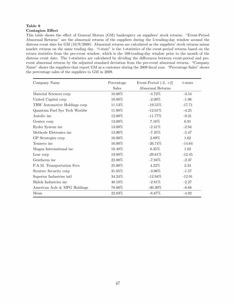
Table 9Contagion EffectThis table shows the effect of General Motors (GM) bankruptcy on suppliers’ stock returns. ‘‘Event-PeriodAbnormal Returns’’ are the abnormal returns of the suppliers during the 5-trading-day window around thedistress event date for GM (10/9/2008). Abnormal returns are calculated as the suppliers’ stock returns minusmarket returns on the same trading day. “t-stats” is the t-statistics of the event-period returns based on thereturn statistics from the pre-event window, which is the 100-trading-day window prior to the month of thedistress event date. The t-statistics are calculated by dividing the differences between event-period and pre-event abnormal returns by the adjusted standard deviation from the pre-event abnormal returns. “CompanyName” shows the suppliers that report GM as a customer during the 2009 fiscal year. “Percentage Sales” showsthe percentage sales of the suppliers to GM in 2009.

Company Name Percentage Event-Period (-2, +2) t-stats

Sales Abnormal Returns

Material Sciences corp 10.00% -4.73% -3.54

United Capital corp 10.80% -2.09% -1.98

TRW Automotive Holdings corp 11.13% -19.55% -17.71

Quantum Fuel Sys Tech Worldw 11.98% -12.01% -4.25

Autoliv inc 12.00% -11.77% -9.31

Gentex corp 13.00% 7.16% 6.91

Ryder System inc 13.00% -2.41% -2.94

Methode Eletronics inc 13.90% -7.35% -5.47

GP Strategies corp 16.00% 2.89% 1.62

Tenneco inc 16.00% -26.74% -14.64

Magna International inc 18.48% 0.35% 1.02

Lear corp 19.80% -29.61% -12.45

Gentherm inc 22.00% -7.94% -2.37

P.A.M. Transportation Svcs 25.00% 4.22% 2.24

Strattec Security corp 31.05% -3.96% -1.57

Superior Industries intl 34.24% -12.94% -12.91

Shiloh Industries inc 40.10% -2.81% -2.27

American Axle & MFG Holdings 78.00% -30.30% -8.88

Mean 22.03% -8.87% -4.92

47

Table 10CDS Spreads of GM’s SuppliersThis table shows the effect of General Motors (GM) bankruptcy on suppliers’ CDS spreads. ‘‘Event-windowCDS Spread’’ is the average CDS spreads of the suppliers during the five-trading-day window around thedistress event date for GM (10/9/2008). CDS spread stand for the spreads on five-year CDS. “Pre-event CDSSpread (10 days)” is the average CDS spreads of suppliers during the ten-day pre-event window, i.e. (–12, –3)trading days prior to the distress event date. “t-statistics” stands for the t-statistics of the event-period returnsbased on the statistics from the pre-event window, calculated by dividing the differences between event-periodand pre-event average CDS spreads by the adjusted standard deviation from the pre-event spreads.

Lear Ryder System TRW Automotive

Event-window CDS Spread 2154.36 208.34 1386.16

Pre-event CDS Spread (10 days) 1313.92 165.48 742.02

Difference 840.44 42.86 644.14

t-statistics 9.86 6.91 15.78

48

Table 11Loan Failure Rate and Customer ConcentrationThis table shows the relation between bank loan failure rates and customer concentration. The dependentvariable is loan failure (LoanFailure), a dummy variable that equals 1 if a firm files for bankruptcy before loanmaturity, 0 otherwise. All regressions use industry-fixed effects and bank-fixed effects. Industry is classified as2-digit SIC industry and the banks are classified by their ultimate parents. Robust z -statistics are shown inparentheses. Columns (1) through (3) show the logit regression results for CustomerSales. Column (4) showsthe OLS result of loan failure for CustomerSales. Columns (5) through (7) show the logit regression results forCustomerSize. Column (8) shows the OLS results of loan failure for CustomerSize.

Dep. Var.: LoanFailure CustomerConcentration is CustomerSales CustomerConcentration is CustomerSize

(1) (2) (3) (4) (5) (6) (7) (8)

CustomerConcentration 1.70 1.77* 1.94* 0.11** 0.20* 0.22** 0.23* 0.01**(1.61) (1.87) (1.70) (2.10) (1.70) (2.00) (1.71) (2.28)

Size 0.47*** 0.47*** 0.33** 0.02** 0.45*** 0.45*** 0.31* 0.02**(3.65) (3.72) (2.07) (2.58) (3.53) (3.58) (1.96) (2.47)

Age -0.02 -0.02 -0.01 -0.00 -0.02 -0.02 -0.01 -0.00(-1.35) (-1.32) (-0.47) (-0.36) (-1.28) (-1.24) (-0.46) (-0.32)

Profitability -7.49*** -7.65*** -9.25*** -0.27** -7.38*** -7.52*** -9.28*** -0.30**(-3.42) (-3.19) (-3.61) (-2.66) (-3.29) (-3.07) (-3.38) (-2.62)

Tangibility 1.56 1.59 1.95 0.11 1.57 1.58 1.93 0.11(1.20) (1.26) (1.38) (1.18) (1.19) (1.25) (1.36) (1.20)

M/B -1.99*** -2.07*** -1.52*** 0.00 -1.97*** -2.05*** -1.47*** 0.00(-3.34) (-3.70) (-3.01) (0.46) (-3.19) (-3.52) (-2.59) (0.64)

Leverage 7.10*** 7.06*** 5.47*** 0.21*** 7.13*** 7.12*** 5.52*** 0.22***(8.86) (11.05) (8.76) (4.04) (8.69) (10.98) (8.76) (4.09)

Ratings 0.76 0.83 0.47 -0.00 0.72 0.80 0.45 -0.00(1.36) (1.52) (0.78) (-0.07) (1.26) (1.42) (0.72) (-0.10)

CreditSpread -1.63*** -2.47*** -0.01 -1.67*** -2.46*** -0.02(-2.63) (-2.96) (-0.67) (-2.64) (-2.93) (-0.82)

TermSpread -0.11 -0.00 -0.01 -0.11 -0.01 -0.01(-0.73) (-0.00) (-0.98) (-0.78) (-0.06) (-0.83)

GDPGrowth -0.12 -0.28 0.00 -0.12 -0.27 0.00(-0.76) (-1.24) (0.53) (-0.73) (-1.18) (0.48)

LoanSpread 0.95*** 0.05*** 0.93*** 0.04***(3.14) (4.58) (3.06) (4.62)

LoanMaturity 1.75*** 0.04*** 1.75*** 0.04***(4.81) (3.61) (4.80) (3.52)

LoanSize 0.27** 0.01 0.27** 0.01(2.47) (0.96) (2.46) (1.07)

LoanType -0.08 0.01 -0.09 0.01(-0.22) (0.93) (-0.25) (0.90)

Observations 2,282 2,282 2,228 2,983 2,242 2,242 2,188 2,903R-squared 0.20 0.20

Robust z -statistics in parentheses*** p-value<0.01, ** p-value<0.05, * p-value<0.10

49

customer concentration and loan contract terms* · customer concentration and loan contract terms*...

Documents