customer density and distribution service costs - … density and distribution service costs . a...
TRANSCRIPT

Customer Density and Distribution Service Costs
A Report Prepared for Hydro One Networks, Inc. by London Economics
International LLC and PowerNex Associates Inc.
November 11th, 2011
390 Bay Street, Suite 1101 27 Ashgrove Place Toronto, Ontario M5H 2Y2 Toronto, Ontario M3B 2Y9 T: (416) 643-6610 T: (416) 487- 4175 F: (416) 643-6611 F: (416) 487- 3706 www.londoneconomics.com www.pnxa.com
Updated: August 29, 2012 EB-2012-0136 Exhibit D-1-1 Attachment 1 Page 1 of 97

Customer Density and Distribution Service Costs
London Economics International LLC ii PowerNex Associates Inc.
Benjamin Grunfeld/Steven Kim Mark Vainberg/Gary Ford/Andrew Poray
(416) 643-6610 (416) 487-4175
[email protected] [email protected]
Executive Summary
London Economics International LLC (“LEI”) and PowerNex Associates Inc. (“PNXA”) were
engaged by Hydro One Networks, Inc. (“HONI”) to study the relationship between customer
density and distribution service costs. This report provides a summary of the analysis that was
conducted as well as observations and conclusions regarding HONI’s existing rate classes and
density weighting factors.
The study was initiated in response to a direction from the Ontario Energy Board (“OEB”)
requiring HONI to provide a detailed analysis on the relationship between density and cost
allocation. The OEB also noted that consideration of alternative density weighting factors and
descriptions and criteria for alternative rate structures should be included in the study.
This engagement had three specific objectives: (i) evaluate the relationship between customer
density and distribution service costs; (ii) assess whether HONI’s existing density based rate
classes and density weighting factors appropriately reflect this relationship; and (iii) consider,
qualitatively, the appropriateness and feasibility of establishing alternative customer class
definitions. The first objective was the primary focus, as feedback from stakeholders suggested
that understanding the relationship between density and cost of service was necessary before
being able to begin to assess the reasonableness of the existing rate classes and cost allocation.
The second and third objectives utilize the results of the analysis that was conducted to address
the first objective.
I. Evaluation of the Relationship between Customer Density and Distribution Service Costs
The first objective was achieved through an econometric analysis of operating area level data
and a direct cost assignment analysis of a selection of sample areas chosen by LEI and PNXA
from across HONI’s distribution service territory.
The econometric study analyzed operations, maintenance, and administrative costs (“OM&A”)
and a proxy for capital costs associated with 48 operating areas within HONI’s distribution
service territory. The purpose of the analysis was to determine whether or not there is a
statistically significant relationship between distribution service costs and customer density
over a five year period from 2006 to 2010, correcting for other factors such as number of
customers, volume of energy delivered etc. As shown in Figure ES1, the estimated coefficients
for customer density, in all four of the models considered, are negative and robust.1 The
coefficients represent the estimated sensitivity (or elasticity) of costs to changes in customer
density, and the negative sign confirms that costs increase as customer density decreases.
1 In statistics terms, this is determined when a coefficient is statistically different from zero at the 95 percent
confidence level.

Customer Density and Distribution Service Costs
London Economics International LLC iii PowerNex Associates Inc.
Benjamin Grunfeld/Steven Kim Mark Vainberg/Gary Ford/Andrew Poray
(416) 643-6610 (416) 487-4175
[email protected] [email protected]
Figure ES1: Estimated Density Coefficients
Source: LEI and PNXA analysis
In the direct cost assignment analysis, 62 sample areas were selected from 11 operating areas
across HONI’s distribution service territory. The sample areas were selected to represent three
levels of density, high, medium, and low (referred to as “HD”, “MD”, and “LD” respectively in
the figures in this report), as well as to capture a representative range of operating conditions.
The purpose of the direct cost assignment study was to analyze the cost to provide service to
customers over a broader spectrum of customer densities than exist at the operating area level.
OM&A costs were directly assigned to the sample areas using “assignment factors” that reflect
engineering practices and utility operations. Capital costs (i.e., non operating costs) were also
taken into consideration through an “asset intensity” calculation for each sample area. Asset
intensity was defined as the replacement cost of the assets serving a sample area divided by the
total number of customers contained within that sample area.
The direct cost assignment analysis confirmed that there is an inverse relationship between
customer density and distribution service costs – consistent with the econometric study results.
As shown in Figure ES2, the mean directly assigned OM&A cost and asset intensity (together
the “assigned costs”) increase as the customer density in the sample areas decrease. The mean
of the assigned costs for each group of low-, medium-, and high-density sample areas were also
shown to be statistically distinct at a 99 percent confidence level.
Figure ES2: Comparison of Sample Area Average Costs
Source: LEI and PNXA analysis
Low High
OM&A CDciircuit-km -0.299 -0.368 -0.23
OM&A CDkm2 -0.100 -0.124 -0.076
OM&A and Capital Proxy CDciircuit-km -0.121 -0.349 -0.225
OM&A and Capital Proxy CDkm2 -0.287 -0.151 -0.092
Costs Modeled in
Econometric Model
Density
Measure
Estimated
Coefficient
95 Percent Confidence Interval
5,244
10,792
27,925
89 156
379
0
100
200
300
400
500
600
-
5,000
10,000
15,000
20,000
25,000
30,000
HD MD LD
OM
&A
Cost
($) p
er
Custo
mer
Asset
Rep
lacem
ent
Cost
($) p
er
Custo
mer
Asset Intensity OM&A Costs

Customer Density and Distribution Service Costs
London Economics International LLC iv PowerNex Associates Inc.
Benjamin Grunfeld/Steven Kim Mark Vainberg/Gary Ford/Andrew Poray
(416) 643-6610 (416) 487-4175
[email protected] [email protected]
Both the econometric analysis and the direct cost assignment analysis established that there is a
statistically significant relationship between customer density and distribution service costs. In
both studies, distribution service costs were shown to decrease as the customer density of on
operating area and/or a sample area increased.
II. Assessment of HONI’s Existing Rate Classes and Density Weighting Factors
The second objective of the study was to assess whether HONI’s existing density based rate
classes and density weighting factors appropriately reflect this relationship. LEI and PNXA
considered three specific elements of HONI’s existing rate structure: (i) the use of customer
density as a differentiator between the rate classes, (ii) the total number of density based rate
classes, and (iii) the density weighting factors used in HONI’s OEB-approved cost allocation
model (“CAM”).
The results of the econometric and direct cost assignment analysis demonstrate that the cost to
serve groups of customers that have different densities is in fact different. As such, on the basis
of cost-causation principles it is appropriate for HONI to use rate classes that are differentiated
based on customer density.
Based on the fact that the mean assigned costs for the three density level sample area groups
were shown to be statistically distinct, it is appropriate for HONI to use three density
differentiated rate classes (a low, medium, and high).
Figure ES3 (OM&A) and Figure ES4 (asset intensity) illustrate the relationship between the
assigned per customer costs and the customer density for each of the samples areas. The two
graphics reveal very similar patterns; the variability of the assigned costs decreases as density
increases. The variability of the assigned costs within a given density group (high, medium,
low) can be taken to represent the degree of cross-subsidisation that could potentially exist.
Variability in the assigned costs is representative of the range of costs associated with serving
individual customers in a group or class. As the range increases, or widens, the average cost to
serve may remain constant, however, the low-cost customers provide a larger subsidy to the
high-cost customers. Conversely, as the range decrease, or tightens, the subsidy diminishes.
There is limited variability in the high-density sample area assigned costs. While there is more
variability across the medium-density sample areas than across the high-density sample areas,
the level of variability in the former is still rather limited. There is considerably more variability
in the assigned costs for the low-density sample areas. This suggests that there may be a greater
degree of cross subsidization within HONI’s lowest-density rate class.

Customer Density and Distribution Service Costs
London Economics International LLC v PowerNex Associates Inc.
Benjamin Grunfeld/Steven Kim Mark Vainberg/Gary Ford/Andrew Poray
(416) 643-6610 (416) 487-4175
[email protected] [email protected]
Figure ES3: Relationship between Assigned per-customer OM&A Costs and Customer Density
Source: LEI and PNXA analysis
Figure ES4: Relationship between Asset Intensity and Customer Density
Source: LEI and PNXA analysis
The direct cost assignment results present the most appropriate window through which to
address the question of whether HONI’s existing density weighting factors accurately reflect
the relationship between customer density and cost of service, as established by the results of
this study. LEI and PNXA chose to assess the reasonableness of the existing density weighting
factors based on the impact they have on the allocation of costs in HONI’s CAM.
Although the direct cost assignment analysis and HONI’s CAM have different starting points
and assumptions for the assignment/allocation of costs, comparisons can be made. Figure ES5
-
200
400
600
800
1,000
1,200
1,400
1,600
1,800
2,000
0 200 400 600 800
OM
&A
Cost
($)
per
Custo
mer
Customers per Square KilometreLD MD HD
-
10,000
20,000
30,000
40,000
50,000
60,000
70,000
0 200 400 600 800
Asset Repla
cem
ent
Cost
($)
per
Custo
mer
Customers per Square KilometreLD MD HD

Customer Density and Distribution Service Costs
London Economics International LLC vi PowerNex Associates Inc.
Benjamin Grunfeld/Steven Kim Mark Vainberg/Gary Ford/Andrew Poray
(416) 643-6610 (416) 487-4175
[email protected] [email protected]
illustrates the ratio of the combined assigned costs between the high-, medium-, and low-
density sample areas and the ratio of per-customer costs allocated to the existing HONI year
round residential rate classes (UR, R1, and R2).2
The ratios are calculated relative to the highest-density group or rate class hence both the high-
density sample area and UR ratios are equal to one. The ratios between the per-customer
allocated costs for HONI’s existing year round residential customer classes are directionally
consistent and of similar magnitude to the ratios obtained in the assigned costs for the low-,
medium-, and high-density sample areas. As is discussed in detail in the body of this report,
the low-density sample areas likely overstate the average density of HONI’s distribution service
territory containing R2 customers. Whereas, the high-density sample areas likely understate the
density of HONI’s distribution service territory containing UR customers. As such, the ratios
between the sample area group means are likely to be lower than they would otherwise be if the
density used in the study was defined in the same manner as the density of the existing HONI
rate classes. Hence, the results of direct cost assignment analysis suggest that the current
density weighting factors likely understate the difference between the costs to serve low- and
high-density customers.
Figure ES5: Comparison of Output from HONI Cost Allocation Model to Adjusted Ratios of Average Sample Area Costs
Source: LEI and PNXA analysis
Based on a review of the 11 operating areas included in the direct cost assignment analysis, the
density of HONI’s service territory containing seasonal customers is expected to fall somewhere
between that of service territory containing the R2 and R1 customers. Similarly, the density of
2 Note that the ratios presented in Figure ES5 are not based directly on the mean sample area assigned costs
presented in Figure ES2. Adjustments have been made to the mean sample area assigned costs to take into account excluded OM&A costs and to combine the OM&A and asset intensity results. A detailed description of these adjustments is provided in Section 5.2 in the body of this report.
1.0
1.7
3.9
1.0
1.6
2.8
-
0.5
1.0
1.5
2.0
2.5
3.0
3.5
4.0
4.5
Direct Cost Assignment Results HONI CAM Results
HD
MD
LD
R2
R1
UR

Customer Density and Distribution Service Costs
London Economics International LLC vii PowerNex Associates Inc.
Benjamin Grunfeld/Steven Kim Mark Vainberg/Gary Ford/Andrew Poray
(416) 643-6610 (416) 487-4175
[email protected] [email protected]
HONI’s service territory containing non-urban general service customers (the GSe and GSd rate
classes) is expected to fall somewhere between that of the service territory containing the R2
and R1 customers, whereas, the density of HONI’s service territory containing urban general
service customers (the UGe and UGd rate classes) is similar to that of the service territory
containing UR customers.
III. Alternative Rate Structures
The third objective of the study is addressed through a qualitative discussion of a number of
alternative rate structures, including: adjustments to HONI’s current rate structure; adopting
the use of municipal boundaries; and province-wide or regional postage–stamp rates.
Based on the results of this study, a wholesale change to HONI’s existing rate class definitions is
not necessary. LEI and PNXA have identified certain adjustments that could be made,
however, any change will result in winners and losers and care will need to be taken to avoid
instances of “rate shock”. While other rate class definitions were considered (i.e., municipal
boundaries or regional rates), the move to such a design is a longer-term decision that LEI and
PNXA suggest should be considered in the context of a broader provincial dialogue.
Customer Density and Distribution Service Costs
London Economics International LLC viii PowerNex Associates Inc.
Benjamin Grunfeld/Steven Kim Mark Vainberg/Gary Ford/Andrew Poray
(416) 643-6610 (416) 487-4175
[email protected] [email protected]
Table of Contents
1 INTRODUCTION ............................................................................................................................. 1
1.1 OBJECTIVES ................................................................................................................................... 1
1.2 PHASED APPROACH AND STAKEHOLDER CONSULTATION ...................................................... 1
1.3 ONTARIO ENERGY BOARD RULINGS .......................................................................................... 2
1.4 STRUCTURE OF ANALYSIS ............................................................................................................ 3
2 DATA SOURCES .............................................................................................................................. 4
3 SUMMARY OF ECONOMETRIC ANALYSIS ........................................................................... 5
3.1 INTRODUCTION ............................................................................................................................ 5
3.2 DATA FOR ECONOMETRIC ANALYSIS ......................................................................................... 6
3.3 FUNCTIONAL FORM ..................................................................................................................... 9
3.4 INCLUDED VARIABLES ............................................................................................................... 10
3.5 ESTIMATION PROCEDURES ........................................................................................................ 11
3.6 RESULTS ...................................................................................................................................... 11
4 SUMMARY OF DIRECT COST ASSIGNMENT ANALYSIS ............................................... 15
4.1 INTRODUCTION .......................................................................................................................... 15
4.2 DATA FOR DIRECT COST ASSIGNMENT ANALYSIS .................................................................. 15
4.3 SELECTION OF OPERATING AND SAMPLE AREAS .................................................................... 16
4.3.1 Operating Area Selection .................................................................................................... 16
4.3.2 Sample Area Selection ......................................................................................................... 19
4.3.3 Summary Characteristics.................................................................................................... 19
4.4 CALCULATING ASSIGNMENT FACTORS .................................................................................... 22
4.5 DIRECT ASSIGNMENT OF OM&A COSTS .................................................................................. 23
4.6 ASSET INTENSITY ....................................................................................................................... 25
4.7 RESULTS ...................................................................................................................................... 26
4.8 IMPACT OF VERY LOW CUSTOMER DENSITY ............................................................................ 29
4.9 DRIVING TIME VERSUS STRAIGHT-LINE DISTANCE ................................................................. 30
5 HONI’S CURRENT TARIFF DESIGN ....................................................................................... 32
5.1 RATE CLASSES AND DEMARCATIONS ....................................................................................... 34
5.1.1 Density as a Differentiator ................................................................................................. 34
5.1.2 Number of Density-based Rate Classes .............................................................................. 35
5.1.3 Demarcation Points ............................................................................................................ 37
5.2 COST ALLOCATION FACTORS ................................................................................................... 37
6 DISCUSSION OF ALTERNATE RATE STRUCTURES ......................................................... 42
6.1.1 Adjustments to HONI’s Existing Structure ...................................................................... 42
6.1.2 Municipal Boundaries ........................................................................................................ 44
6.1.3 Regional Rates .................................................................................................................... 45
7 CONCLUSIONS AND RECOMMENDATIONS ..................................................................... 48
APPENDIX A –ECONOMETRIC ANALYSIS DETAILS ............................................................... 49
INTRODUCTION TO ECONOMETRIC ANALYSIS ..................................................................................... 49

Customer Density and Distribution Service Costs
London Economics International LLC ix PowerNex Associates Inc.
Benjamin Grunfeld/Steven Kim Mark Vainberg/Gary Ford/Andrew Poray
(416) 643-6610 (416) 487-4175
[email protected] [email protected]
SAMPLE OPERATING AREA DATA ........................................................................................................ 49
APPENDIX B – BACKGROUND INFORMATION ON DISTRIBUTION SYSTEMS ............. 52
DISTRIBUTION SYSTEM TOPOLOGY AND EQUIPMENT ......................................................................... 52
OPERATION AND MAINTENANCE OF DISTRIBUTION SYSTEMS ........................................................... 55
APPENDIX C – DIRECT COST ASSIGNMENT ANALYSIS DETAILS ..................................... 58
SAMPLE AREA MAPS ............................................................................................................................. 58
ASSIGNMENT FACTOR CALCULATION METHODOLOGY ..................................................................... 68
INDIVIDUAL SAMPLE AREA ASSIGNMENT FACTORS ........................................................................... 70
INDIVIDUAL SAMPLE AREA RESULTS ................................................................................................... 71
ADDITIONAL SCATTER PLOTS ............................................................................................................... 73
ESTIMATED DENSITY OF EXISTING RATE CLASSES ............................................................................... 74
List of Figures
FIGURE 1: OPERATING AREAS IN HONI’S DISTRIBUTION SERVICE TERRITORY ...................................... 5
FIGURE 2: GRANULARITY OF HONI DATA ................................................................................................ 7
FIGURE 3: ECONOMETRIC PARAMETER ESTIMATES (OM&A COSTS MODEL WITH CUSTOMER PER
CIRCUIT KILOMETRE) ................................................................................................................... 12
FIGURE 4: ECONOMETRIC PARAMETER ESTIMATES (OM&A COST MODEL WITH CUSTOMER PER
SQUARE KILOMETRE) .................................................................................................................... 12
FIGURE 5: ECONOMETRIC PARAMETER ESTIMATES (OM&A COSTS AND CAPITAL PROXY MODEL
WITH CUSTOMER PER CIRCUIT KILOMETRE) ............................................................................... 13
FIGURE 6: ECONOMETRIC PARAMETER ESTIMATES (OM&A COSTS AND CAPITAL PROXY MODEL
WITH CUSTOMER PER SQUARE KILOMETRE) ............................................................................... 13
FIGURE 7: ESTIMATED DENSITY COEFFICIENTS ........................................................................................ 13
FIGURE 8: OPERATING AREAS SELECTED FROM NORTHERN ONTARIO ................................................. 17
FIGURE 9: OPERATING AREAS SELECTED FROM SOUTHERN ONTARIO .................................................. 18
FIGURE 10: SUMMARY CHARACTERISTICS OF INDIVIDUAL SAMPLE AREAS .......................................... 20
FIGURE 11: SUMMARY CHARACTERISTICS OF ALL SAMPLE AREAS ........................................................ 21
FIGURE 12: SUMMARY CHARACTERISTICS OF 11 OPERATING AREAS IN STUDY .................................... 21
FIGURE 13: MAPPING OF OM&A COST CATEGORIES AND ASSIGNMENT FACTORS ............................. 24
FIGURE 14: ANNUALIZED PER-CUSTOMER VEGETATION COSTS FOR ALL SAMPLE AREAS................... 25
FIGURE 15: REPLACEMENT COST USED TO CALCULATE ASSET INTENSITY ............................................ 26
FIGURE 16: COMPARISON OF SAMPLE AREA MEAN COSTS .................................................................... 27
FIGURE 17: DISTRIBUTION OF PER-CUSTOMER ASSIGNED SAMPLE AREA OM&A COSTS ..................... 28
FIGURE 18: DISTRIBUTION OF ASSET INTENSITY RESULTS ....................................................................... 28
FIGURE 19: SUMMARY OF STATISTICAL ANALYSIS .................................................................................. 29
FIGURE 20: PER-CUSTOMER RESULTS FOR VERY LOW DENSITY SAMPLE AREA .................................... 29
FIGURE 21: PERCENT CHANGE IN DIRECTLY ASSIGNED PER-CUSTOMER OM&A COSTS ..................... 31
FIGURE 22: COMPONENTS OF STANDARD DISTRIBUTION TARIFF DESIGN ............................................. 32
FIGURE 23: STRUCTURE OF HONI’S CURRENT DISTRIBUTION RATE CLASSES ...................................... 33
FIGURE 24: RELATIONSHIP BETWEEN PER-CUSTOMER ASSIGNED OM&A COSTS AND CUSTOMER
DENSITY ......................................................................................................................................... 36

Customer Density and Distribution Service Costs
London Economics International LLC x PowerNex Associates Inc.
Benjamin Grunfeld/Steven Kim Mark Vainberg/Gary Ford/Andrew Poray
(416) 643-6610 (416) 487-4175
[email protected] [email protected]
FIGURE 25: RELATIONSHIP BETWEEN PER-CUSTOMER ASSET REPLACEMENT COST AND CUSTOMER
DENSITY ......................................................................................................................................... 36
FIGURE 26: RESULTS OF HONI COST ALLOCATION MODEL .................................................................. 38
FIGURE 27: UNADJUSTED RATIO OF AVERAGE SAMPLE AREA COSTS .................................................... 39
FIGURE 28: ADJUSTED RATIO OF AVERAGE SAMPLE AREA COSTS ......................................................... 40
FIGURE 29: COMPARISON OF OUTPUT FROM HONI CAM TO ADJUSTED RATIOS OF AVERAGE
SAMPLE AREA COSTS ................................................................................................................... 41
FIGURE 30: LOW-DENSITY SAMPLE AREA OM&A COSTS ...................................................................... 43
FIGURE 31: LOW-DENSITY SAMPLE AREA ASSET INTENSITY .................................................................. 43
FIGURE 32: SUMMARY OF A REGIONAL RATE MECHANISM ................................................................... 46
FIGURE 33: LDCS IN THE NIAGARA REGION ........................................................................................... 47
FIGURE 34: OPERATING AREA 2010 CUSTOMER DENSITY (PER SQUARE KILOMETRE)........................... 49
FIGURE 35: OPERATING AREA 2010 CUSTOMER DENSITY (PER CIRCUIT KILOMETRE)........................... 50
FIGURE 36: OPERATING AREA 2010 OM&A COST .................................................................................. 50
FIGURE 37: OPERATING AREA 2010 CAPITAL PROXY .............................................................................. 51
FIGURE 38: SIMPLIFIED GENERATION/TRANSMISSION/DISTRIBUTION MODEL ................................... 52
FIGURE 39: TYPICAL SINGLE PHASE POLE-TOP TRANSFORMER ............................................................. 53
FIGURE 40: TYPICAL OPEN AIR DISTRIBUTION STATION ........................................................................ 54
FIGURE 41: SINGLE PHASE VOLTAGE REGULATOR (LEFT) AND THREE PHASE SERIES INDUCTOR
(RIGHT) .......................................................................................................................................... 55
FIGURE 42: TYPICAL RADIAL FEEDER TOPOLOGY IN NORTHERN ONTARIO ......................................... 56
FIGURE 43: GRID-LIKE FEEDER TOPOLOGY TYPICAL IN SOUTHERN ONTARIO ...................................... 57
FIGURE 44: TYPICAL OFF ROAD RIGHTS OF WAY .................................................................................... 57
FIGURE 45: BRACEBRIDGE OPERATING AREA MAP ................................................................................. 58
FIGURE 46: DRYDEN OPERATING AREA MAP .......................................................................................... 59
FIGURE 47: ESSEX OPERATING AREA MAP ............................................................................................... 60
FIGURE 48: KINGSTON OPERATING AREA MAP....................................................................................... 61
FIGURE 49: NEWMARKET OPERATING AREA MAP .................................................................................. 62
FIGURE 50: OWEN SOUND OPERATING AREA MAP ................................................................................ 63
FIGURE 51: PERTH OPERATING AREA MAP ............................................................................................. 64
FIGURE 52: PETERBOROUGH OPERATING AREA MAP ............................................................................. 65
FIGURE 53: SIMCOE OPERATING AREA MAP............................................................................................ 66
FIGURE 54: SUDBURY OPERATING AREA MAP ......................................................................................... 67
FIGURE 55: TIMMINS OPERATING AREA MAP ......................................................................................... 68
FIGURE 56: INDIVIDUAL SAMPLE AREA ASSIGNMENT FACTORS (2010) ................................................ 70
FIGURE 57: LOW-DENSITY SAMPLE AREA RESULTS ................................................................................ 71
FIGURE 58: MEDIUM-DENSITY SAMPLE AREA RESULTS .......................................................................... 72
FIGURE 59: HIGH-DENSITY SAMPLE AREA RESULTS ............................................................................... 73
FIGURE 60: RELATIONSHIP BETWEEN OM&A COSTS AND CUSTOMER DENSITY (PER CIRCUIT
KILOMETRE) ................................................................................................................................... 73
FIGURE 61: RELATIONSHIP BETWEEN ASSET INTENSITY AND CUSTOMER DENSITY (PER CIRCUIT
KILOMETRE) ................................................................................................................................... 74
FIGURE 62: CUSTOMER DENSITY DISTRIBUTION FOR HONI’S UR RATE CLASS IN 11 OPERATING
AREAS ............................................................................................................................................ 74

Customer Density and Distribution Service Costs
London Economics International LLC xi PowerNex Associates Inc.
Benjamin Grunfeld/Steven Kim Mark Vainberg/Gary Ford/Andrew Poray
(416) 643-6610 (416) 487-4175
[email protected] [email protected]
FIGURE 63: CUSTOMER DENSITY DISTRIBUTION FOR HONI’S R1 RATE CLASS IN 11 OPERATING
AREAS ............................................................................................................................................ 75
FIGURE 64: CUSTOMER DENSITY DISTRIBUTION FOR HONI’S R2 RATE CLASS IN 11 OPERATING
AREAS ............................................................................................................................................ 75
FIGURE 65: CUSTOMER DENSITY DISTRIBUTION FOR HONI’S SEASONAL RATE CLASS IN 11
OPERATING AREAS ....................................................................................................................... 75
FIGURE 66: CUSTOMER DENSITY DISTRIBUTION FOR HONI’S UGE AND UGD RATE CLASSES IN 11
OPERATING AREAS ....................................................................................................................... 76
FIGURE 67: CUSTOMER DENSITY DISTRIBUTION FOR HONI’S GSE AND GSD RATE CLASSES IN 11
OPERATING AREAS ....................................................................................................................... 76

Customer Density and Distribution Service Costs
London Economics International LLC 1 PowerNex Associates Inc.
Benjamin Grunfeld/Steven Kim Mark Vainberg/Gary Ford/Andrew Poray
(416) 643-6610 (416) 487-4175
[email protected] [email protected]
1 Introduction
London Economics International LLC (“LEI”) and PowerNex Associates Inc. (“PNXA”) were
engaged by Hydro One Networks, Inc. (“HONI”) to study the relationship between customer
density and distribution service costs. This report provides a summary of the analysis
conducted as well as observations and conclusions regarding HONI’s existing rate classes and
density weighting factors.
This report contains six sections, in addition to this introduction:
Data Sources;
Summary of the Econometric Analysis;
Summary of the Direct Cost Assignment Analysis;
Implications for HONI's Current Tariff Design;
Discussion of Alternate Rate Structures; and
Conclusions and Recommendations.
Three appendices to this report provide additional details on the econometric analysis;
background information on distribution systems; and additional details on the direct cost
assignment analysis, including maps of the operating areas and sample areas selected and
individual sample area results.
1.1 Objectives
LEI and PNXA had three specific objectives.
Objective 1: Evaluate the relationship between customer density and distribution
service costs.
Objective 2: Assess whether HONI’s existing density based rate classes and density
weighting factors appropriately reflect this relationship.
Objective 3: Consider, qualitatively, the appropriateness and feasibility of establishing
alternate customer class definitions.
The first objective was the primary focus, as feedback from stakeholders suggested that
understanding the relationship between customer density and distribution service cost was
necessary before being able to begin to assess the reasonableness of the existing rate classes and
density weighting factors.
1.2 Phased Approach and Stakeholder Consultation
LEI and PNXA were engaged by HONI in two phases. The first phase of the engagement was a
“scoping” phase. LEI and PNXA utilized this phase to develop and refine the proposed study
methodology. The second phase of the engagement was an “implementation” phase. LEI and
PNXA utilized this phase to implement the study methodology.
The first phase consisted of four main tasks. The first task was to review background material
relevant to HONI’s distribution rate design, including its existing CAM and recent regulatory

Customer Density and Distribution Service Costs
London Economics International LLC 2 PowerNex Associates Inc.
Benjamin Grunfeld/Steven Kim Mark Vainberg/Gary Ford/Andrew Poray
(416) 643-6610 (416) 487-4175
[email protected] [email protected]
filings. The second task involved the collection and analysis of HONI and third-party data to
understand the extent of data available to support the detailed study methodology. The third
task involved the development and validation of a detailed study methodology. The fourth
task was to present the proposed study methodology to stakeholders.
The stakeholder information session was held on March 22, 2011, at HONI’s offices in Toronto,
Ontario. Stakeholders provided a number of comments, which have been incorporated into the
methodology discussed in this report. The presentation delivered by LEI and PNXA, and notes
from the stakeholder session are available online from HONI’s website.3
The study also takes into consideration comments from the September 8, 2010, stakeholder
session in Toronto, Ontario, in particular feedback regarding the need to understand the
density-cost relationship before deciding what to do about rate classes.4
1.3 Ontario Energy Board Rulings
The Ontario Energy Board (“OEB”) issued its Decision with Reasons in regards to HONI’s 2008
distribution rate application on December 18, 2008. In this decision, HONI was directed to
“provide a more detailed analysis on the relationship between density and cost
allocation to the Board. [The analysis] should consider whether the number of
Residential and General Service customer classes in the new class structure is
adequate, and whether the customer class demarcations approved in this Decision
offer the best reflection of cost causation. The study should include consideration
of alternative density weightings, with descriptions and criteria for comparing
alternatives”.5
In HONI’s 2010/11 rate application (EB-2009-0096), HONI submitted a preliminary report that
conceptually explored the relationship between density and cost allocation.6 The study did not
attempt to address the relationship quantitatively. The Decision with Reasons issued by the
OEB directed HONI to comply with the prior direction on this issue and noted that
“The [OEB] expects [HONI] to work cooperatively with the parties but leaves it
to [HONI’s] discretion to determine how best to conduct the study taking into
consideration timing, feasibility and cost.”
3 Presentation: <http://www.hydroone.com/RegulatoryAffairs/Documents/EB-2011-
0215/Dx%20Stakeholder%20Cost%20Density%20LEI-PNXA%20Presentation.pdf> Session Notes: <http://www.hydroone.com/RegulatoryAffairs/Documents/EB-2011-0215/Density%20Stakeholder%20Consultation%20Meeting%20Notes.pdf >
4 Session Notes: <http://www.hydroone.com/RegulatoryAffairs/Documents/EB-2011-
0215/Density%20Stakeholder%20Consultation%20Meeting%20Notes.pdf> 5 OEB. “In the matter of an application by: Hydro One Networks, Inc. 2008 Rates - Decision with Reasons”. (EB-
2007-0681). Toronto: December 18, 2008. 6 Elenchus Research Associates. “Principles for Defining and Allocating Costs to Density-Based Sub-Classes”.
Toronto: 2009.

Customer Density and Distribution Service Costs
London Economics International LLC 3 PowerNex Associates Inc.
Benjamin Grunfeld/Steven Kim Mark Vainberg/Gary Ford/Andrew Poray
(416) 643-6610 (416) 487-4175
[email protected] [email protected]
This study’s methodology, developed by LEI and PNXA, serves to meet the requirements of the
OEB decisions and reflect stakeholder input. In particular, the study evaluates the relationship
between customer density and distribution service costs, and assesses whether the existing rate
classes and density-based weighting factors reflect this relationship. Furthermore, recognizing
that there is no unique best solution in rate design, this report discusses the appropriateness
and feasibility of establishing alternative customer class definitions.
1.4 Structure of Analysis
The methodology LEI and PNXA used to complete its analysis, which was presented to
stakeholders on March 22, 2011, has two distinct components: an econometric analysis and a
direct cost assignment analysis.
The econometric analysis provides valuable insights into the relationship between customer
density and distribution service costs at the operating area level. As such, a significant amount
of the variability in customer density that is observed across HONI’s service territory is not
available in this type of analysis as it is averaged out.
On the other hand, the direct cost assignment method is able to drill down to a much greater
level of detail and analyze smaller sample areas with a wider range of observed customer
densities than the econometric analysis. Furthermore, the results of the direct cost assignment
analysis, as discussed in Section 5 of this report, are useful in addressing the second objective of
this engagement.
The two methods offer unique but complimentary ways of analyzing the relationship between
customer density and distribution service costs. The results of each were not known at the time
the methodology was developed and the intention was always to utilize both, together, to
support the conclusions and recommendations in this report.
Customer Density and Distribution Service Costs
London Economics International LLC 4 PowerNex Associates Inc.
Benjamin Grunfeld/Steven Kim Mark Vainberg/Gary Ford/Andrew Poray
(416) 643-6610 (416) 487-4175
[email protected] [email protected]
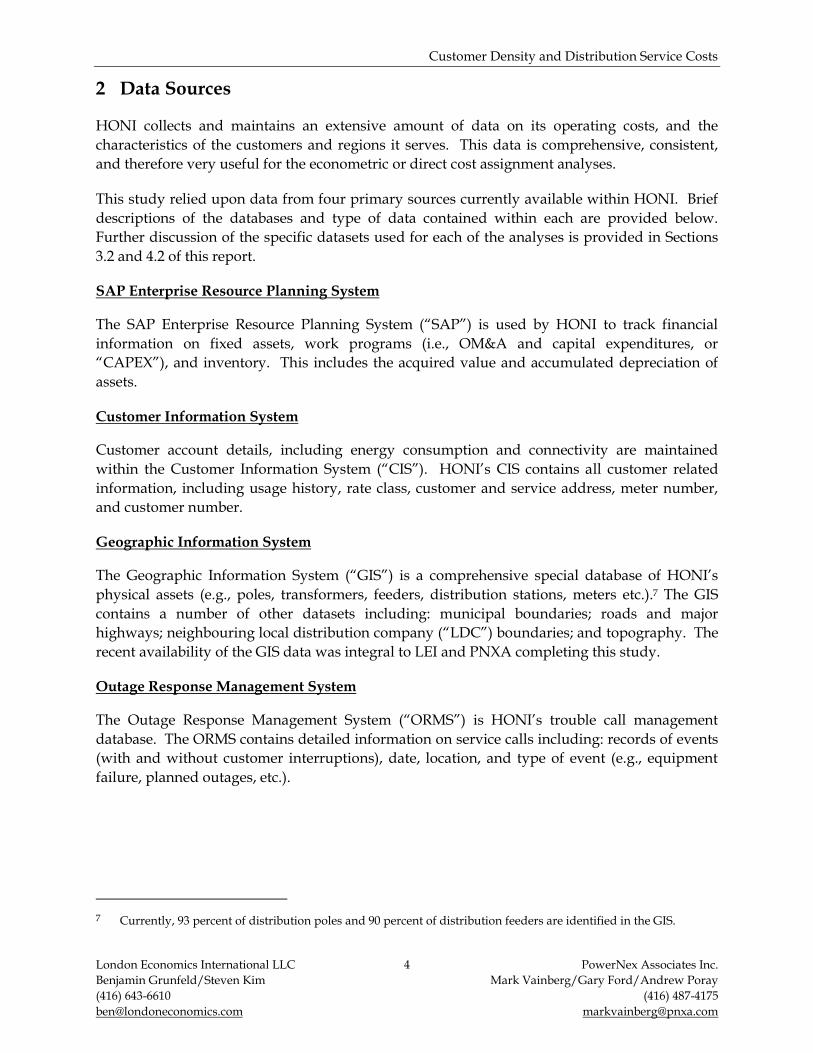
2 Data Sources
HONI collects and maintains an extensive amount of data on its operating costs, and the
characteristics of the customers and regions it serves. This data is comprehensive, consistent,
and therefore very useful for the econometric or direct cost assignment analyses.
This study relied upon data from four primary sources currently available within HONI. Brief
descriptions of the databases and type of data contained within each are provided below.
Further discussion of the specific datasets used for each of the analyses is provided in Sections
3.2 and 4.2 of this report.
SAP Enterprise Resource Planning System
The SAP Enterprise Resource Planning System (“SAP”) is used by HONI to track financial
information on fixed assets, work programs (i.e., OM&A and capital expenditures, or
“CAPEX”), and inventory. This includes the acquired value and accumulated depreciation of
assets.
Customer Information System
Customer account details, including energy consumption and connectivity are maintained
within the Customer Information System (“CIS”). HONI’s CIS contains all customer related
information, including usage history, rate class, customer and service address, meter number,
and customer number.
Geographic Information System
The Geographic Information System (“GIS”) is a comprehensive special database of HONI’s
physical assets (e.g., poles, transformers, feeders, distribution stations, meters etc.).7 The GIS
contains a number of other datasets including: municipal boundaries; roads and major
highways; neighbouring local distribution company (“LDC”) boundaries; and topography. The
recent availability of the GIS data was integral to LEI and PNXA completing this study.
Outage Response Management System
The Outage Response Management System (“ORMS”) is HONI’s trouble call management
database. The ORMS contains detailed information on service calls including: records of events
(with and without customer interruptions), date, location, and type of event (e.g., equipment
failure, planned outages, etc.).
7 Currently, 93 percent of distribution poles and 90 percent of distribution feeders are identified in the GIS.

Customer Density and Distribution Service Costs
London Economics International LLC 5 PowerNex Associates Inc.
Benjamin Grunfeld/Steven Kim Mark Vainberg/Gary Ford/Andrew Poray
(416) 643-6610 (416) 487-4175
[email protected] [email protected]
3 Summary of Econometric Analysis
As mentioned in Section 1.4, one component of the methodology was an econometric analysis of
operating area level data. LEI and PNXA carried out an econometric analysis of OM&A and a
proxy for capital costs associated with the 48 operating areas within HONI’s distribution service
territory. The purpose of this analysis was to demonstrate whether or not there is a statistically
significant relationship between distribution service costs and customer density, correcting for
other factors.
3.1 Introduction
One definition of econometrics (the science of econometric analysis) is that it is “the process of
fitting mathematical economic models to real-world data”.8 In the context of this study, LEI and
PNXA developed and estimated an economic model to explain the variability in distribution
service costs across the operating areas within HONI’s service territory, over a five year period.
Figure 1: Operating Areas in HONI’s Distribution Service Territory
Note: The highlighted operating areas are those included in the direct cost assignment analysis. The econometrics analysis included data for all operating areas Source: HONI
The functional form of the econometric model, in this case a “cost function”, is chosen based on
theory. The unknown parameters embedded within the cost function are then estimated using
regression analysis.
8 Stock, J. and M. Watson. Introduction to Econometrics. New York: Pearson Education, Inc. Book.

Customer Density and Distribution Service Costs
London Economics International LLC 6 PowerNex Associates Inc.
Benjamin Grunfeld/Steven Kim Mark Vainberg/Gary Ford/Andrew Poray
(416) 643-6610 (416) 487-4175
[email protected] [email protected]
Regression analysis includes techniques for modeling and analyzing the relationship between
independent (causal or explanatory) variables and dependent variables. More specifically,
regression analysis provides insight into how the value of a dependent variable changes when
one of the independent variables changes (assuming all other independent variables are held
constant). Econometric analysis is a commonly accepted practice within utility regulatory
proceedings. While certain elements of the analysis can lead to contention (for example, the
reasonableness of the underlying data, choice of parameters, model definition, etc.), the
approach and the methods behind the concept are generally well accepted.
In Ontario, econometric analysis was accepted by the OEB as part of the second- and third-
generation incentive rate mechanism (“2GIRM” and “3GIRM”, respectively) proceedings.9 In
these proceedings it was used to benchmark utility cost performance and establish relative
productivity trends across peer groups. There are also numerous examples from other
jurisdictions across North America where econometric analysis has been relied upon in the
context of distribution rate design.10
In this study, LEI and PNXA relied entirely on data pertaining to a single utility, HONI. As will
be discussed in the next section, this approach goes a long way to eliminating one of the more
common concerns with inter-utility cost studies.
3.2 Data for Econometric Analysis
A common point of contention that has arisen in Ontario around the use of econometric
analysis, generally speaking, is the potential for inconsistent datasets as a result of different
reporting standards across utilities. The OEB has taken steps to standardize reporting
requirements in Ontario, but there are still areas where data is limited and concerns can arise
(e.g., the treatment of shared services, different capitalization rules, etc.). The use of data
exclusively from HONI eliminates this concern. LEI and PNXA understand that HONI
maintains consistent data reporting and tracking standards across its entire service territory.
The data that LEI and PNXA relied upon for the econometric analysis comes from three
primary systems within HONI, namely SAP, GIS and CIS. For the purposes of this econometric
analysis, the operating area name acts as a primary key to link data from each of the
independent data systems.
The majority of this data is available and was compiled at the operating area level.11 The
exceptions were:
9 EB-2006-0089 and EB-2007-0673 10 An abridged list of examples include: a study performed by Power Systems Engineering for the Illinois Citizens
Utility Board, which evaluated the cost performance of Ameren Illinois Company; in 2009, Oklahoma Gas & Electric conducted a benchmarking study to gauge operating and maintenance cost performance; and in 2003, Ameren Missouri provided evidence in support of its cost performance using econometric techniques.
11 For some operating areas (e.g., Thunder Bay) data was compiled by aggregating sub-regions (e.g., Thunder Bay,
Marathon and Geraldton).

Customer Density and Distribution Service Costs
London Economics International LLC 7 PowerNex Associates Inc.
Benjamin Grunfeld/Steven Kim Mark Vainberg/Gary Ford/Andrew Poray
(416) 643-6610 (416) 487-4175
[email protected] [email protected]
vegetation management costs, which are tracked on a feeder basis;
distribution station costs, which are tracked at the provincial level;
a handful of other OM&A work program costs that are also tracked at the provincial
level;
Customer Care costs, which are tracked at the provincial level; and
Shared Services and general and administrative costs which are also tracked at the
provincial level.
HONI provided datasets for the past five years (2006 through 2010) for the 48 operating areas.
Figure 2: Granularity of HONI Data
Number of Customers
HONI provided data from the CIS consisting of the number of customers in each of the rate
classes in 2006 to 2010, by operating area.
Energy Consumption
Energy consumption data was provided by HONI for each of the existing rate classes within
each operating area from 2006 through 2010.
OM&A Costs
OM&A costs within HONI are tracked through work programs. The two prominent sets of
programs within the distribution company are lines and stations. The annual OM&A cost for
each year and for each operating area was calculated as the total of the Lines OM&A, Stations
OM&A, and vegetation management costs, the latter being a subset of Lines OM&A but tracked
independently.
The majority (approximately 90 percent) of the Lines OM&A costs are naturally tracked by
HONI at the operating area level, including costs associated with storms and trouble calls.
Rather than assigning provincial-level costs to the operating areas, Lines OM&A costs that are
tracked at the provincial level were excluded from the analysis.
• Distribution
stations OM&Aand CAPEX
• Shared services
• Customer care• Operations
• Number of
customers• Energy
consumption
• Lines OM&A and CAPEX
• Acquired asset value
• Cumulative
depreciation• Asset counts
• Geographic data
• Vegetation
management
Provincial Operating Area Feeder

Customer Density and Distribution Service Costs
London Economics International LLC 8 PowerNex Associates Inc.
Benjamin Grunfeld/Steven Kim Mark Vainberg/Gary Ford/Andrew Poray
(416) 643-6610 (416) 487-4175
[email protected] [email protected]
Stations OM&A costs are all tracked at the provincial level. As such, total provincial stations
OM&A costs were disaggregated to the operating areas based on the number of distribution
stations within each operating area.
Vegetation management costs are reported within HONI at the distribution-feeder level. HONI
provided details on the specific feeders contained within each operating area and the annual
vegetation costs associated with each feeder over the past ten years. Given that vegetation costs
can vary from year to year, LEI and PNXA calculated a ten-year levelized cost for each feeder.12
The levelized feeder cost was calculated by inflating all of the annual feeder costs into 2010
dollars, using actual values of the Canadian consumer price index, and then taking an average.
The feeder level costs were then aggregated to produce a total cost for each operating area in
2010 dollars. The levelized operating area cost was then adjusted for inflation to determine the
annual levelized cost in nominal 2006, 2007, 2008, and 2009 dollars. This approach results in a
smooth vegetation management cost for each year within a given operating area, while at the
same time maintains the variability in vegetation management costs across different operating
areas.
Econometric studies are based on observations of data from real world situations. Minimizing
the number of adjustments to the data typically results in more robust and defensible results.
With the exception of distribution stations OM&A and CAPEX, LEI and PNXA did not allocate
provincial level costs to the operating areas for the econometric analysis. Hence, the majority of
customer care costs, shared services, and operations expenses which are all tracked at the
provincial level were excluded.
Total Capital Costs
There are a number of possible measures of “capital costs” for a distribution utility, for example
both the net book value (“NBV”) and replacement cost of all installed assets are plausible
proxies.
For the purpose of this econometric study, LEI and PNXA developed an estimate of the annual
depreciation and the return on regulated asset base associated with each operating area in each
year (a “Capital Proxy”). This approach is reflective of the annual capital-driven costs that are
embedded in HONI’s distribution revenue requirement.
To develop this Capital Proxy, LEI and PNXA used data from SAP on the acquired value and
the accumulated depreciation of assets in each operating area. SAP tracks groups of similar
assets in an operating area rather than the individual assets themselves. It also maintains
records of the year in which groups of assets were placed into service (asset vintage). The
difference between the acquired value and accumulated depreciation yields the net book value
for each asset vintage.
12 The vegetation management cost data reflected the historical ten years average vegetation management cycle
across HONI’s service territory.

Customer Density and Distribution Service Costs
London Economics International LLC 9 PowerNex Associates Inc.
Benjamin Grunfeld/Steven Kim Mark Vainberg/Gary Ford/Andrew Poray
(416) 643-6610 (416) 487-4175
[email protected] [email protected]
The capital cost measure for each operating area was calculated as the average of the end of
year and beginning of year NBV, which takes into account annual capital additions in each year,
times the OEB approved weighted average cost of capital (“WACC”) for HONI in each year,
plus the total depreciation taken in the year.
Equation 1
Other Asset and Geographic Data
HONI also provided additional data on the total number of assets within the operating areas.
Specifically, and critical to this study, this included the total length of all feeders within the
operating area and the physical size of the operating area. Additional data such as the number
of distribution stations, number and rating of transformers was also made available.
Customer Density
LEI and PNXA calculated the customer density of each operating area from the customer count
data and the asset and geographic data provided for each operating area for each year. Two
parameters were calculated: (i) the total number of customers per square kilometre of the
operating area and (ii) the total number of customers per circuit kilometre (including overhead,
underground, and submarine feeders) of feeders in the operating area.13 The customer densities
represent an average for each of the operating areas.
Charts summarizing the operating area level data collected and used in the econometric
analysis are provided in Appendix A.
3.3 Functional Form
The functional form used in this analysis is similar to those used in other econometric analysis
performed in Ontario in relation to distribution utility costs. It is the same functional form that
was used by Pacific Economics Group in its work for the OEB as part of the 2GIRM and 3GIRM
proceedings.14,15 The chosen functional form is “quadratic” and has the following general
formula.16
13 The total size of the operating area and the total length of conductor were only available for 2010. 14 Pacific Economics Group. “Second Generation Incentive Regulation for Ontario Power Distributors.” 2006. 15 Pacific Economics Group. “Sensitivity Analysis on Efficiency Ranking and Cohorts for the 2009 Year: Update.”
2008. 16 The “double log” form is one of the simplest functional forms used when analyzing utility costs, as it assumes
constant economies of scale. The double log form works with smaller datasets. The quadratic form is an expansion of the double log form. The quadratic form contains exponential terms which adjust for varying economies of scale and scope and non-linear relationships between dependent and independent variables. Typically a larger data sample is required when using this form. The “translog” form is a further expansion of

Customer Density and Distribution Service Costs
London Economics International LLC 10 PowerNex Associates Inc.
Benjamin Grunfeld/Steven Kim Mark Vainberg/Gary Ford/Andrew Poray
(416) 643-6610 (416) 487-4175
[email protected] [email protected]
Equation 2
Here, “Yi” denotes a variable that quantifies output and “Wi” denotes an input price. The “Z”
variable denotes additional business conditions, “T”
error term. The “a” and “b” terms represent the estimated coefficients. Note, that because each
of the independent and dependent variables is represented as a natural logarithm (“ln”) the
coefficients are “elasticity” estimates.17
LEI and PNXA analyzed two specific cost functions, one where C denotes OM&A costs only
and the other where C denotes OM&A and the Capital Proxy.
3.4 Included Variables
The refining of the cost function was an iterative process, where a number of different model
specifications were tested. In determining which variables to include in a final model,
economists weigh concerns such as the sign of the estimated coefficients, the statistical
significance of the coefficients, and the overall “fit” of the regression.
It is important that the sign of the coefficients in the model be consistent with logical
expectations. It is also important that the estimated coefficients be statistically significant.
Statistically significant implies that with a high degree of confidence the coefficient is non-zero.
Fit is most commonly measured by the “R-squared” of the regression -- a value from zero to
one, with one being a perfect fit. The R-squared term measures the magnitude of the error
between the predicted values and the actual values.
In addition, in order to obtain robust estimated coefficients, it is important to utilize
independent variables that have a limited degree of multicollinearity. Multicollinearity occurs
when one or more of the independent variables are correlated. Multicollinearity causes erratic
results, as the model is not able to uniquely isolate the impact of the independent variables on
the dependent variable.
The four parameters determined to produce the best fit cost function were customer density
(“CD”), number of customers (“N”), energy density (“ED”), and a time, or trend, variable (“T”).
Energy density is the average consumption per customer in each operating area. No input
the quadratic form. Translog functions allow for interaction between independent variables. The form also takes into account varying economies of scale and scope. The translog form is generally more flexible in terms of describing costs than the quadratic or double log functions. The translog form also requires a larger data sample than the quadratic or double log functional forms.
17 Elasticity represents the ratio of change of one variable with respect to another. It is used to measure the
responsiveness of the dependent variable to changes to an independent variable.

Customer Density and Distribution Service Costs
London Economics International LLC 11 PowerNex Associates Inc.
Benjamin Grunfeld/Steven Kim Mark Vainberg/Gary Ford/Andrew Poray
(416) 643-6610 (416) 487-4175
[email protected] [email protected]
prices were considered as the input prices within HONI are generally the same across the
operating areas. Number of customers is an output variable, thus the final model also includes
its square term (“NN”). The inclusion of the square term allows for the modeling of a non-
linear relationship between cost and number of customers. This choice of variables is consistent
with other econometric analyses where customer density is considered as an independent
variable.18,19
It should be noted that other operating area level data was considered for the analysis including
asset age, net asset value, assets counts (distribution stations, transformers), conductor length,
average customer distance from the service centre(s) and geography. The inclusion of these
variables did not improve the results of the regression. The inclusion of additional variables
resulted in erratic model behaviour, such as sign changes and lack of significance of the
estimated coefficients. This is likely due to the overall size of the sample and the fact that many
of the characteristic variables are correlated.
As will be discussed in Section 3.6, the simpler model specification produced robust and
consistent results.
3.5 Estimation Procedures
Ordinary least squares (“OLS”) is a method for estimating the unknown variables in a linear
regression model. An OLS model seeks to minimize the sum of the squared differences
between the observed values and the predicated values as determined by the regression. OLS is
commonly used in econometric and engineering applications. OLS models typically work well
when multicollinearity is minimized and when the model errors are homoskedastic.20
Generalized least squares (“GLS”) is similar to OLS, except it is typically applied when the
variances of the observations are unequal (i.e., there is heteroscedasticity), or when there is a
certain degree of correlation between the observations.
LEI and PNXA utilized a modified GLS algorithm to estimate the regression coefficients.
3.6 Results
The following four figures summarize the results of the regression analysis. Figure 3 and
Figure 4 show the results of the model which considered OM&A costs only with density
measured as number of customers per circuit kilometre and number of customers per square
kilometre, respectively. Since a logarithmic form was used, the estimated coefficients are a
measure of elasticity. The t-statistic is the ratio of the parameter estimate and the standard
18 Lawrence, Denis. Meyrick and Associates. “Efficiency Comparisons of Australian and New Zealand Gas
Distribution Businesses Allowing for Operating Environment Differences.” 2007. 19 Farsi, M.; Filippini, M.; Plagnet, M.; Saplacan, R..Centre for Energy Policy and Economics, Swiss Federal
Institutes of Technology. “The Economies of Scale in the French Power Distribution Utilities.” 2010. 20 Homoskedasticity occurs when the variances of the error term is not correlated with one of the variables of the
function. If the variances of the error term are correlated with one or more of the variables of the function, the error terms are said to be heteroskedastic.

Customer Density and Distribution Service Costs
London Economics International LLC 12 PowerNex Associates Inc.
Benjamin Grunfeld/Steven Kim Mark Vainberg/Gary Ford/Andrew Poray
(416) 643-6610 (416) 487-4175
[email protected] [email protected]
error. With 240 observations, a t-statistic in excess of an absolute value of 1.96 suggests that the
explanatory variable is statistically significant at the 95 percent confidence level.
Figure 3: Econometric Parameter Estimates (OM&A Costs Model with Customer per Circuit Kilometre)
Source: LEI and PNXA analysis
The estimated coefficients in both models are statistically different from zero at the 95 percent
confidence level, and exhibit signs that are consistent with the fundamental understanding of
the costs of a distribution utility. For example, the model results show that as the number of
customers served increases, the OM&A costs are expected to increase. Also, as the average size
of a customer increases, as measured by the energy density term, the model predicts that
OM&A costs would decrease.
Figure 4: Econometric Parameter Estimates (OM&A Cost Model with Customer per Square Kilometre)
Source: LEI and PNXA analysis
Figure 5 and Figure 6 show the results of the model that considered both OM&A costs and the
Capital Proxy with density measured as number of customers per circuit kilometre and number
of customers per square kilometre, respectively.
240
0.73
2006-2010
Explanatory Variable
N
NN
CDline-km
ED
T
-0.109 -3.31
0.021 2.22
Number of Observations:
R2:
Sample Period:
3.756 4.79
-0.297 -3.83
-0.299 -8.47
Parameter Estimate T-Statistic
240
0.73
2006-2010
Explanatory Variable
N
NN
CDkm2
ED
T
-0.072 -2.07
0.018 1.95
5.072 6.65
-0.426 -5.66
-0.100 -8.01
Number of Observations:
R2:
Sample Period:
Parameter Estimate T-Statistic

Customer Density and Distribution Service Costs
London Economics International LLC 13 PowerNex Associates Inc.
Benjamin Grunfeld/Steven Kim Mark Vainberg/Gary Ford/Andrew Poray
(416) 643-6610 (416) 487-4175
[email protected] [email protected]
Figure 5: Econometric Parameter Estimates (OM&A Costs and Capital Proxy Model with Customer per Circuit Kilometre)
Source: LEI and PNXA analysis
In these models the estimated coefficient for the energy density term is not significantly
different from zero at the 95 percent level. The estimated coefficients for the customer density
variables remain negative and significantly different from zero at the 95 percent level.
Figure 6: Econometric Parameter Estimates (OM&A Costs and Capital Proxy Model with Customer per Square Kilometre)
Source: LEI and PNXA analysis
The following table summarizes the estimated density coefficients and the 95 percent
confidence intervals for the four models.
Figure 7: Estimated Density Coefficients
Source: LEI and PNXA analysis
The results shown in Figure 7 indicate that for a fivefold increase in the number of customers
per square kilometre (e.g. an increase from 5 to 25 customers per square kilometre), all else
being equal, costs (both OM&A and capital) would be expected to decrease by 143.5 percent.
240
0.71
2006-2010
Explanatory Variable
N
NN
CDline-km
ED
T
-0.026 -0.61
-0.023 2.05
3.975 4.80
-0.305 -3.80
-0.287 -9.10
Number of Observations:
R2:
Sample Period:
Parameter Estimate T-Statistic
240
0.74
2006-2010
Explanatory Variable
N
NN
CDkm2
ED
T
0.028 0.64
0.020 1.88
5.596 5.74
-0.460 -4.93
-0.121 -7.94
Number of Observations:
R2:
Sample Period:
Parameter Estimate T-Statistic
Low High
OM&A CDciircuit-km -0.299 -0.368 -0.23
OM&A CDkm2 -0.100 -0.124 -0.076
OM&A and Capital Proxy CDciircuit-km -0.121 -0.349 -0.225
OM&A and Capital Proxy CDkm2 -0.287 -0.151 -0.092
Costs Modeled in
Econometric Model
Density
Measure
Estimated
Coefficient
95 Percent Confidence Interval

Customer Density and Distribution Service Costs
London Economics International LLC 14 PowerNex Associates Inc.
Benjamin Grunfeld/Steven Kim Mark Vainberg/Gary Ford/Andrew Poray
(416) 643-6610 (416) 487-4175
[email protected] [email protected]
To put the magnitude of the increase in density into perspective, in the direct cost assignment
analysis the high-density sample areas were 6.8 times denser on average than the medium-
density sample areas. The medium-density sample areas were 7.2 times denser on average than
the low-density sample areas.
The 95 percent confidence interval of the density coefficient in all four models exclude zero.
Thus the model demonstrates that customer density, regardless of how it is measured, is
inversely related to distribution service costs. As customer density decreases, the cost to serve
the same number of customers, all other factors being equal, would be expected to increase.
The opposite also holds true where customer density increases, the cost to serve the same
number of customers, holding all other variables constant, would be expected to decrease.
The first objective of this study was to analyze the relationship between customer density and
distribution service costs. The econometric analysis confirms that there is a statistically
significant relationship, and that as customer density increases cost generally decrease, all else
held equal. With this understanding, the direct cost assignment analysis described in the next
chapter of this report attempts to confirm or refute this relationship at a more granular sample
area level within selected operating areas. The direct cost assignment analysis also aims to
explore the magnitude of the density-cost relationship.

Customer Density and Distribution Service Costs
London Economics International LLC 15 PowerNex Associates Inc.
Benjamin Grunfeld/Steven Kim Mark Vainberg/Gary Ford/Andrew Poray
(416) 643-6610 (416) 487-4175
[email protected] [email protected]
4 Summary of Direct Cost Assignment Analysis
4.1 Introduction
In the first phase of this engagement, the feasibility of a direct cost assignment analysis was
investigated. The conclusion of that work established that such an analysis was feasible, and,
when tested in one operating area, provided results which were considered by LEI and PNXA
to be credible. In the second phase of this engagement, the direct cost assignment analysis was
extended to 62 sample areas selected from 11 operating areas across HONI’s distribution service
territory.
The purpose of the direct cost assignment analysis was to investigate how the cost to serve
customers over a broad range of customer densities varies. Sample areas were selected to
represent three levels of density high, medium, and low (referred to as “HD”, “MD”, and “LD”
respectively in the figures in this report), as well as to capture a representative range of the
normal operating conditions that exist across HONI’s service territory.
OM&A costs were directly assigned to the sample areas using a number of “assignment factors”
that reflect engineering practices and utility operations. The assignment factors were selected
based on an understanding of distribution system operations, types of assets, topology, and
hence the principal drivers of cost.21 This assignment of OM&A costs allowed for the
calculation of a per-customer OM&A cost for each sample area.
The “asset intensity” was also calculated for each sample area, as a proxy for capital (non-
operating) costs. Asset intensity was defined as the replacement cost of the assets serving a
sample area divided by the total number of customers contained within that sample area.
4.2 Data for Direct Cost Assignment Analysis
The direct cost assignment analysis utilized a number of datasets from within HONI. A brief
description of the major datasets collected is provided below.
The number and length of distribution feeders, whether they pass through a sample
area, and the length inside and outside each operating area and sample area.
The number of customers in each sample area and operating area.
The number of poles in each sample area and each operating area, including pole
ownership (e.g., HONI-owned, Bell Canada owned, customer-owned, etc.) and type of
pole mount (i.e., rock, earth, other).22
The total number and type of assets (e.g., transformers, switches, regulators, capacitors,
re-closers, meters, etc.) in each sample area and operating area.
21 Background information on distribution systems and common terminology can be found in Appendix B. 22 It is quite common for utilities to share poles. HONI and Bell Canada have a pole sharing agreement in a
number of locations across the province. Typically the owner of the pole is responsible for ongoing maintenance.

Customer Density and Distribution Service Costs
London Economics International LLC 16 PowerNex Associates Inc.
Benjamin Grunfeld/Steven Kim Mark Vainberg/Gary Ford/Andrew Poray
(416) 643-6610 (416) 487-4175
[email protected] [email protected]
The geographic coordinates of customers, poles, and service centers in each sample area
and operating area.
The number of interruptions and non-interruptions resulting from both storm and non-
storm related events for each operating area and each feeder.23
OM&A costs for each operating area and provincial-level programs.
The typical replacement cost of assets currently used across HONI’s network.
4.3 Selection of Operating and Sample Areas
Operating areas were selected to be representative of the range of conditions across HONI’s
distribution service territory. The number of sample areas is important to assure the statistical
significance of the results. Based on the preliminary results from the initial phase of the
engagement, LEI and PNXA estimated that, at a minimum, 45 sample areas would likely be
required to achieve a reasonable degree of confidence in the results.
4.3.1 Operating Area Selection
To provide for a broad coverage of HONI’s service territory a total of 11 operating areas were
selected: Bracebridge, Dryden, Essex, Kingston, Newmarket, Owen Sound, Perth, Peterborough,
Simcoe, Sudbury, and Timmins.
HONI operates across diverse terrain with a large variation in environmental, geographic, and
other operating conditions. The operating areas were chosen to ensure that they represent a
material cross section of the actual conditions, customers, and geography of HONI’s service
territory. Figure 8 and Figure 9 illustrate the chosen operating areas and their location across
the province. The operating areas selected, include three in the north, three in the southwest,
three from the central part of the province, and two in the east. They include a blend of
agricultural, forested, and urban areas. Furthermore, the operating areas were selected to
represent diversity in terms of geology, the prevalence of storms, and overall size.
23 Non-interruptions refer to trouble calls where a work crew was dispatched but customers did not suffer a loss of
power.

Customer Density and Distribution Service Costs
London Economics International LLC 17 PowerNex Associates Inc.
Benjamin Grunfeld/Steven Kim Mark Vainberg/Gary Ford/Andrew Poray
(416) 643-6610 (416) 487-4175
[email protected] [email protected]
Figure 8: Operating Areas Selected from Northern Ontario
Source: HONI; LEI and PNXA analysis

Customer Density and Distribution Service Costs
London Economics International LLC 18 PowerNex Associates Inc.
Benjamin Grunfeld/Steven Kim Mark Vainberg/Gary Ford/Andrew Poray
(416) 643-6610 (416) 487-4175
[email protected] [email protected]
Figure 9: Operating Areas Selected from Southern Ontario
Source: HONI; LEI and PNXA analysis

Customer Density and Distribution Service Costs
London Economics International LLC 19 PowerNex Associates Inc.
Benjamin Grunfeld/Steven Kim Mark Vainberg/Gary Ford/Andrew Poray
(416) 643-6610 (416) 487-4175
[email protected] [email protected]
4.3.2 Sample Area Selection
A total of 62 sample areas were selected; between four and seven from each of the 11 operating
areas.
In order to test the hypothesis that there is a relationship between customer density and the cost
to serve customers, sample areas having three distinct customer densities were defined. This
was accomplished by using sample areas of approximately the same size and by selecting areas
with varying numbers of customers. The selection of sample areas did not consider the existing
rate classes or density definitions. When selecting the sample areas, LEI and PNXA followed
the five general guidelines listed below:
each sample area should be of a similar size, approximately 20 square kilometres;
low-density sample areas should have between 100 and 200 customers;
medium-density sample areas should have between 700 and 1,200 customers;
high-density sample areas were found around any large “urban” concentration of
customers within the operating area, resulting in sample areas with typically more than
2,000 customers.
sample area boundaries should be selected to minimize the impact of network structure
on the calculation of the assignment factors and/or asset intensity.
With respect to the last guideline, it was important to minimize the degree of judgment
required to determine whether an asset served, or an outage affected, a given sample area.
The above criteria were formulated and used for the initial identification of potential sample
areas. Additional low-density sample areas with fewer customers (i.e., less than 100) were also
included to better capture the actual variability of customer density in rural areas.
The process of selecting operating areas and sample areas within them was carried out by LEI
and PNXA.
4.3.3 Summary Characteristics
Summary characteristics for each of the individual sample areas, including the number of
customers, area, total circuit kilometres, and customer density are provided in Figure 10. The
smallest sample area contained 20 customers while the largest contained over 13,000. Customer
density, measured as customers per square kilometre, ranges from 0.7 to 667.9. Likewise,
customer density, measured as customers per circuit kilometre, ranges for 0.4 to 79.5.
Figure 11 provides a summary of the sample area characteristics, by density class (i.e., low,
medium, or high). The average customer density of the low-density sample areas is 6
customers per square kilometre or 3 customers per circuit kilometre. The average customer
density of the medium-density sample areas is 43 customers per square kilometre or 16
customers per circuit kilometre. The average for the high-density sample areas is 291 customers
per square kilometre or 40 customers per circuit kilometre.

Customer Density and Distribution Service Costs
London Economics International LLC 20 PowerNex Associates Inc.
Benjamin Grunfeld/Steven Kim Mark Vainberg/Gary Ford/Andrew Poray
(416) 643-6610 (416) 487-4175
[email protected] [email protected]
Figure 10: Summary Characteristics of Individual Sample Areas
Source: HONI; LEI and PNXA analysis
By design, the average customer-per-square-kilometre densities of the sample area groupings
are distinct and there is no overlap at the individual sample area level. For example, within the
Operating Area Sample Area Number of Customers km2
Circuit km Customers per km2
Customers per Circuit km
Bracebridge LD1 154 18.2 25.7 8.5 6.0
Bracebridge LD2 102 21.4 27.9 4.8 3.6
Bracebridge LD3 111 19.2 31.9 5.8 3.5
Bracebridge MD1 1,125 21.7 94.5 51.9 11.9
Bracebridge MD2 1,417 22.5 74.7 62.9 19.0
Bracebridge MD3 727 28.8 77.2 25.2 9.4
Dryden LD1 103 22.4 43.4 4.6 2.4
Dryden LD2 20 29.4 47.9 0.7 0.4
Dryden MD1 872 16.9 43.5 51.6 20.1
Dryden MD2 1,057 17.4 65.0 60.7 16.3
Dryden HD1 3,608 22.7 106.1 158.8 34.0
Essex LD1 179 22.8 38.0 7.8 4.7
Essex LD2 174 15.0 73.9 11.6 2.4
Essex MD1 886 21.0 49.4 42.2 17.9
Essex MD2 912 17.9 44.7 50.9 20.4
Essex HD1 2,279 20.9 95.1 109.2 24.0
Essex HD2 1,973 20.5 111.7 96.1 17.7
Kingston LD1 84 19.3 36.9 4.4 2.3
Kingston LD2 84 18.8 34.8 4.5 2.4
Kingston MD1 662 22.8 52.2 29.1 12.7
Kingston MD2 858 24.0 63.1 35.7 13.6
Kingston HD1 11,260 16.9 237.3 667.9 47.5
Newmarket LD1 259 17.4 56.6 14.9 4.6
Newmarket LD2 271 19.4 33.8 14.0 8.0
Newmarket LD3 164 18.5 21.7 8.9 7.6
Newmarket MD1 911 16.7 68.7 54.4 13.3
Newmarket HD1 3,593 16.5 91.2 218.1 39.4
Newmarket HD2 8,956 18.0 170.6 498.7 52.5
Newmarket HD3 8,463 17.2 168.2 492.7 50.3
Newmarket HD4 3,876 21.3 145.7 181.9 26.6
Owen Sound LD1 78 19.7 22.1 4.0 3.5
Owen Sound LD2 63 17.4 30.7 3.6 2.1
Owen Sound MD1 598 22.0 76.7 27.2 7.8
Owen Sound MD2 514 19.5 75.2 26.3 6.8
Owen Sound HD1 10,062 22.4 237.9 448.7 42.3
Perth LD1 92 20.7 37.6 4.4 2.4
Perth LD2 130 20.6 33.2 6.3 3.9
Perth MD1 810 24.3 69.5 33.3 11.7
Perth MD2 547 24.8 80.1 22.0 6.8
Perth HD1 3,811 17.5 132.4 217.5 28.8
Perth HD2 5,366 20.5 193.9 261.2 27.7
Peterborough LD1 126 24.4 64.8 5.2 1.9
Peterborough LD2 162 24.7 54.7 6.6 3.0
Peterborough MD1 949 20.1 58.9 47.2 16.1
Peterborough MD2 1,182 20.9 71.6 56.5 16.5
Peterborough MD3 1,237 23.2 63.5 53.4 19.5
Simcoe LD1 153 20.9 25.2 7.3 6.1
Simcoe LD2 128 20.5 40.3 6.2 3.2
Simcoe MD1 938 24.4 54.8 38.5 17.1
Simcoe MD2 936 13.2 17.5 70.9 53.6
Simcoe MD3 446 20.0 34.9 22.3 12.8
Sudbury LD1 137 18.2 32.2 7.5 4.3
Sudbury LD2 90 19.5 30.9 4.6 2.9
Sudbury MD1 938 22.2 57.0 42.2 16.4
Sudbury MD2 808 20.5 52.0 39.4 15.5
Sudbury HD1 4,674 21.5 106.4 217.7 43.9
Sudbury HD2 3,361 20.3 100.2 165.7 33.5
Sudbury HD3 2,032 24.2 51.4 83.9 39.5
Timmins LD1 123 20.9 25.8 5.9 4.8
Timmins LD2 39 24.2 26.8 1.6 1.5
Timmins HD1 13,057 19.7 164.2 663.5 79.5
Timmins HD2 2,983 17.4 55.1 171.1 54.1
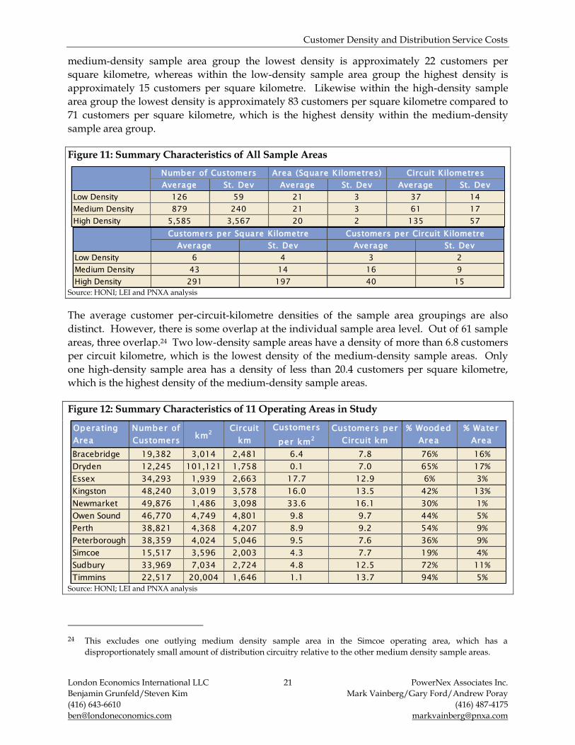
Customer Density and Distribution Service Costs
London Economics International LLC 21 PowerNex Associates Inc.
Benjamin Grunfeld/Steven Kim Mark Vainberg/Gary Ford/Andrew Poray
(416) 643-6610 (416) 487-4175
[email protected] [email protected]
medium-density sample area group the lowest density is approximately 22 customers per
square kilometre, whereas within the low-density sample area group the highest density is
approximately 15 customers per square kilometre. Likewise within the high-density sample
area group the lowest density is approximately 83 customers per square kilometre compared to
71 customers per square kilometre, which is the highest density within the medium-density
sample area group.
Figure 11: Summary Characteristics of All Sample Areas
Source: HONI; LEI and PNXA analysis
The average customer per-circuit-kilometre densities of the sample area groupings are also
distinct. However, there is some overlap at the individual sample area level. Out of 61 sample
areas, three overlap.24 Two low-density sample areas have a density of more than 6.8 customers
per circuit kilometre, which is the lowest density of the medium-density sample areas. Only
one high-density sample area has a density of less than 20.4 customers per square kilometre,
which is the highest density of the medium-density sample areas.
Figure 12: Summary Characteristics of 11 Operating Areas in Study
Source: HONI; LEI and PNXA analysis
24 This excludes one outlying medium density sample area in the Simcoe operating area, which has a
disproportionately small amount of distribution circuitry relative to the other medium density sample areas.
Average St. Dev Average St. Dev Average St. Dev
Low Density 126 59 21 3 37 14
Medium Density 879 240 21 3 61 17
High Density 5,585 3,567 20 2 135 57
Number of Customers Area (Square Kilometres) Circuit Kilometres
Average St. Dev Average St. Dev
Low Density 6 4 3 2
Medium Density 43 14 16 9
High Density 291 197 40 15
Customers per Square Kilometre Customers per Circuit Kilometre
Operating
Area
Number of
Customerskm
2Circuit
km
Customers
per km2
Customers per
Circuit km
% Wooded
Area
% Water
Area
Bracebridge 19,382 3,014 2,481 6.4 7.8 76% 16%
Dryden 12,245 101,121 1,758 0.1 7.0 65% 17%
Essex 34,293 1,939 2,663 17.7 12.9 6% 3%
Kingston 48,240 3,019 3,578 16.0 13.5 42% 13%
Newmarket 49,876 1,486 3,098 33.6 16.1 30% 1%
Owen Sound 46,770 4,749 4,801 9.8 9.7 44% 5%
Perth 38,821 4,368 4,207 8.9 9.2 54% 9%
Peterborough 38,359 4,024 5,046 9.5 7.6 36% 9%
Simcoe 15,517 3,596 2,003 4.3 7.7 19% 4%
Sudbury 33,969 7,034 2,724 4.8 12.5 72% 11%
Timmins 22,517 20,004 1,646 1.1 13.7 94% 5%

Customer Density and Distribution Service Costs
London Economics International LLC 22 PowerNex Associates Inc.
Benjamin Grunfeld/Steven Kim Mark Vainberg/Gary Ford/Andrew Poray
(416) 643-6610 (416) 487-4175
[email protected] [email protected]
This differentiation between the sample areas groups (i.e. the lack of high-, medium-, and low-
density sample areas with overlapping customer densities) contributes to the robustness of the
study by limiting boundary concerns.
Figure 12 provides the same data as Figure 11, but for each of the 11 operating areas as a whole.
As evident, the selected operating areas reflect a broad range of defining characteristics,
including size, total circuit length, density, wood cover, and water cover.
4.4 Calculating Assignment Factors
A total of seven distinct assignment factors were developed. A brief description of each
assignment factor is provided below and the detailed method for determining the assignment
factors is provided in Appendix C. In addition to the individual assignment factors, LEI and
PNXA used combined factors. The combined factors were calculated by multiplying individual
assignment factors.
Customer Ratio across Entire HONI Service Territory (“CRT”)
This assignment factor represents the proportion of the total number of HONI customers across
the entire service territory contained within an individual sample area. It is used to assign
certain provincial-level OM&A costs.
Customer Ratio within each Operating Area (“CROA”)
This assignment factor represents the proportion of the total number of HONI customers in a
given operating area contained within an individual sample area. It is used to assign certain
operating area OM&A costs.
Customer Distance Ratio (“CDR”)
This ratio represents the total distance to the customers in a sample area relative to the total
distance to all customers in the operating area. The purpose of this ratio was to assign
operating area level OM&A costs to customers in each sample area, recognizing that work
crews typically have to travel some distance to customer locations to carry out specific tasks.
The ratio is based on “straight-line” distances between customers and the closest service centre,
which is an approximation of the actual time it takes for a work crew to reach a given customer.
Underground Conductor Ratio (“UGR”)
The purpose of this ratio was to assign operating area level OM&A costs related to
underground cables. It represents the proportion of the kilometres of underground cable in a
sample area relative to the total operating area.
Pole Distance Ratio (all poles) (“PDRT”)
This ratio represents the total distance to the poles in a sample area relative to the total distance
to all poles in the operating area. The purpose of this ratio was to assign asset related operating
area level OM&A costs to each sample area, recognizing that crews typically have to travel

Customer Density and Distribution Service Costs
London Economics International LLC 23 PowerNex Associates Inc.
Benjamin Grunfeld/Steven Kim Mark Vainberg/Gary Ford/Andrew Poray
(416) 643-6610 (416) 487-4175
[email protected] [email protected]
some distance to get to an asset to carry out specific tasks. Examples of this would include
repairing or replacing poles or conductor after storm damage. Similar to the customer distance
ratio, this assignment factor is based on the straight-line distance between an asset and the
service center as an approximation for the time it takes a work crew to reach an asset.
LEI and PNXA performed a sensitivity analysis to determine whether straight-line distance was
a reasonable approximation for estimated driving time. The results of this analysis are
provided in Section 4.9.
Interruption Ratio Non- Storms (“IRNS”)
The purpose of this ratio was to assign operating area level trouble call related work program
costs that are non-storm related. It represents the proportion of non-storm related trouble calls
(interruptions and non-interruptions) in an operating area that relate to an individual sample
area.
Interruption Ratio Storms (“IRS”)
The purpose of this ratio was to assign operating area level trouble call related work program
costs that are storm related. It reflects the proportion of storm related trouble calls
(interruptions and non-interruptions) in an operating area that relate to an individual sample
area.
Detailed calculation methodologies as well as the specific sample area assignment factors are
provided in Appendix C. It should be noted that 2010 data (customer counts, asset counts,
replacement costs) was used to develop the assignment factors, with the exception of
interruption ratios, which were calculated for each specific year based on the interruption/non-
interruption data for that year.
4.5 Direct Assignment of OM&A Costs
OM&A costs were directly assigned to individual sample areas on the basis of the assignment
factors discussed above. The direct cost assignment analysis focused primarily on OM&A
expenses related to sustainment activities. Sustainment activities include distribution line
maintenance, distribution station maintenance, and vegetation management. Sustainment
activities represented approximately 57 percent of HONI’s estimated 2010 OM&A
expenditure.25
The OM&A costs that were included in the direct cost assignment analysis provide a reasonable
basis for assessing whether there is a relationship between distribution service costs and
customer density. The balance of the OM&A costs are customer care, shared services,
operations, and development related, and as such are generally not expected to vary on a per-
customer basis with density. However, as described in Section 5, it is necessary to take these
25 HONI. “Cost of Service Summary: Exhibit C1, Tab 1, Schedule 1 (EB-2009-0096)”. September 2009.

Customer Density and Distribution Service Costs
London Economics International LLC 24 PowerNex Associates Inc.
Benjamin Grunfeld/Steven Kim Mark Vainberg/Gary Ford/Andrew Poray
(416) 643-6610 (416) 487-4175
[email protected] [email protected]
costs into consideration when analyzing the existing rate classes and the appropriateness of the
existing density weighting factors.
OM&A costs are generally tracked at one of three levels: provincial (e.g., engineering services,
etc.); operating area (e.g., line patrols and asset maintenance, etc.); or by feeder (i.e., vegetation
management). Certain assignment factors could be directly applied to provincial-level costs, for
example customer distance ratio. Other assignment factors are only relevant to operating area
level costs. Figure 13 summarizes the specific assignment factors that were used to assign the
range of OM&A costs considered.
Figure 13: Mapping of OM&A Cost Categories and Assignment Factors
Source: LEI and PNXA analysis
LEI and PNXA collected OM&A cost data for a total of five years (2006 through 2010).
Originally available in nominal dollar values, the annual data was adjusted to 2010 dollar
values using the Canadian consumer price index. As will be discussed in more detail in the
context of the results, this allowed for averaging across years.
Vegetation management costs were assigned to the sample areas in a slightly different manner.
Vegetation processes in HONI address tree clearing and brush control on a planned and
proactive basis. Historic cost data for tree clearing and brush control covering a 10-year period
were provided by HONI for the feeders that serve customers in the sample areas that were
selected. The annual cost data was put on a common 2010 dollar basis using the Canadian
consumer price index. Brush control and tree clearing costs were totalled and divided by 10,
the historical average duration of a clearing cycle, to provide a levelized annual vegetation
control cost for each feeder.26
The total length of the feeders and the length of the feeders within each sample area were
obtained from the GIS. The total vegetation control costs for each sample area were then
26 Vegetation control cycles vary across the province. HONI recommended the use of 10 years as it reflects the
historical average for the entire service territory.
OM&A Cost Category Assignment Factor
Cable Locates UGR
Corrective Maintenance PDRT
Customer Disconnects and Reconnects CDR
Distribution Lines Patrol PDRT
Field Meter Reading and Ancillary Services, inc. Meter Replacement CDR
Field Collections and Special Investigations CDR
Sentinel Light Maintenance CDR
Small External Demand Requests CDR
Wood Pole Testing PDRT
Trouble Calls IRNS*PDRT
Storm Maintenance Costs IRS*PDRT
Distribution Station Operation and Maintenance Costs CROA
Provincial Level Operation and Maintenance Costs CRT

Customer Density and Distribution Service Costs
London Economics International LLC 25 PowerNex Associates Inc.
Benjamin Grunfeld/Steven Kim Mark Vainberg/Gary Ford/Andrew Poray
(416) 643-6610 (416) 487-4175
[email protected] [email protected]
calculated as a proportion of the total feeder cost equivalent to the proportion of the total length
of feeder within the sample area.27 Vegetation management costs (on a per-customer basis) for
each of the sample areas are plotted against the density of the sample area in Figure 14.
Figure 14: Annualized per-customer Vegetation Costs for All Sample Areas
Source: HONI; LEI and PNXA analysis
4.6 Asset Intensity
The asset intensity analysis estimates the replacement cost of existing HONI distribution assets
attributable to the individual sample areas. Assets located within the sample areas were
identified using the GIS. Based on current replacement costs, the total value of assets used to
serve a sample area was calculated. The total replacement cost value was then divided by the
total number of customers in the sample to obtain the per-customer replacement cost (the “asset
intensity”).
The choice of replacement cost as opposed to another proxy for capital cost such as net book
value is not expected to have a material impact on the results. LEI and PNXA do not have
reason to believe that the assets serving low-density sample areas are consistently older or
newer than the assets serving medium- or high-density sample areas. Statistical analysis of
operating area level data compiled for the econometric analysis suggests that there is only a
weak correlation (< 0.3) between age and customer density.
Note that the asset intensity analysis is based on the number of assets physically located within
the sample areas. This assumption tends to lead to lower asset intensity results for sample areas
that are remote from distribution stations, as typically there would be a long radial feeder and
other assets outside of such sample areas that are used to serve customers in these areas.
Conversely, high-density areas are typically located in proximity to a distribution station and all
27 M Class feeders passing through the sample areas were also included in this calculation.
0
100
200
300
400
500
600
700
800
0 100 200 300 400 500 600 700 800Annual
Veg
eta
tion M
anag
em
ent
Cost
($) p
er
Custo
mer
Customers per Square KilometreLD MD HD
1,500~

Customer Density and Distribution Service Costs
London Economics International LLC 26 PowerNex Associates Inc.
Benjamin Grunfeld/Steven Kim Mark Vainberg/Gary Ford/Andrew Poray
(416) 643-6610 (416) 487-4175
[email protected] [email protected]
the equipment serving customers in the high-density area is more likely to be physically located
within the high-density sample area.
The replacement costs of assets used in this study are summarized in Figure 15. The costs
reflect the average cost to replace typical assets in use by HONI across a wide range of
conditions.
Figure 15: Replacement Cost used to Calculate Asset Intensity
Source: HONI; LEI and PNXA analysis
Costs associated with both the high- and low-voltage distribution stations were assigned to all
customers served by the distribution station. The proportion of the distribution station
replacement cost attributable to an individual sample area was calculated based on the
proportion of the total number customers supplied from the distribution station that are
physically located within the sample area.
4.7 Results
The annual results for the individual sample areas for 2006 through 2010 were averaged to
minimize the impact of the cyclical nature of some work programs on the study results.
The low-density sample area assigned OM&A costs range from $89 to $1,868 per customer, with
a mean value of $379. The medium-density sample area assigned OM&A costs range from $83
to $342 per customer, with mean value of $156. The high-density sample area assigned OM&A
costs range from $56 to $157 per customer, with mean value of $89.
The low-density sample area asset intensities range from $7,083 to $61,279 per customer, with a
mean value of $27,925. The medium-density sample area asset intensities range from $4,848 to
$18,338 per customer, with mean value of $10,792. The high-density sample area OM&A costs
range from $2,265 to $9,037 per customer, with mean value of $5,244. Individual sample area
results are provided in Figure 57, Figure 58, and Figure 59 in Appendix C.
Asset Replacement Cost
High Voltage Distribution Station $3,500,000
Low Voltage Distribution Station $2,500,000
Transformer $4,700
Pole $7,350
Overhead Conductor (per km) $1,000
Underground Cable (per km) $10,000
Submarine Cable (per km) $56,000
Regulator $7,750
Recloser $7,750
Capacitor $8,600
Fuse $100
Switch $30,000
Smart Meter $100
Smart Meter Repeater $250
Smart Meter Collector $1,800

Customer Density and Distribution Service Costs
London Economics International LLC 27 PowerNex Associates Inc.
Benjamin Grunfeld/Steven Kim Mark Vainberg/Gary Ford/Andrew Poray
(416) 643-6610 (416) 487-4175
[email protected] [email protected]
As can be seen in Figure 16, each sample area group appears to have a distinct mean value for
both OM&A and asset intensity. The mean value of the high-density sample areas appears to
be lower than the mean value for the medium-density sample areas, which in turn is lower than
the mean value for the low-density sample areas.
Figure 16: Comparison of Sample Area Mean Costs
Source: LEI and PNXA analysis
As discussed above, there are a range of costs associated with the high-, medium-, and low-
density sample areas. Plots of the distribution (histograms) of the low-, medium-, and high-
density sample area results, for both OM&A costs (Figure 17) and asset intensity (Figure 18),
reveal that there is some overlap.
With this overlap present, further analysis was required to determine if the mean values of the
distributions are in fact different, from a statistical standpoint. That is, could it be reasonably
concluded that the high-density sample area mean value is different and less than the medium-
density sample area mean value, and similarly when comparing the high- and low-density and
medium- and low-density sample area mean values.
5,244
10,792
27,925
89 156
379
0
100
200
300
400
500
600
-
5,000
10,000
15,000
20,000
25,000
30,000
HD MD LD
OM
&A
Cost
($) p
er
Custo
mer
Asset
Rep
lacem
ent
Cost
($) p
er
Custo
mer
Asset Intensity OM&A Costs

Customer Density and Distribution Service Costs
London Economics International LLC 28 PowerNex Associates Inc.
Benjamin Grunfeld/Steven Kim Mark Vainberg/Gary Ford/Andrew Poray
(416) 643-6610 (416) 487-4175
[email protected] [email protected]
Figure 17: Distribution of per-customer Assigned Sample Area OM&A Costs
Source: LEI and PNXA analysis
Figure 18: Distribution of Asset Intensity Results
Source: LEI and PNXA analysis
The t-test was used to determine if the distributions of the low-, medium-, and high-density
sample area results could have come from the same underlying population or not, and with
what confidence a conclusion could be stated. The calculation was carried out with the
hypothesis that the two sample area result distributions were drawn from the same underlying
population.
When the t-test was applied to the low-density and medium-density OM&A results, at the 99
percent confidence level the t-statistic was 3.014. This implies that the probability of the
0%
10%
20%
30%
40%
50%
60%
70%
80%
50
10
0
15
0
20
0
25
0
30
0
35
0
40
0
45
0
50
0
55
0
60
0
65
0
70
0
75
0
80
0
85
0
90
0
95
0
10
00
OM&A Cost per CustomerLD MD HD
0%
10%
20%
30%
40%
50%
60%
0
2,5
00
5,0
00
7,5
00
10
,00
0
12
,50
0
15
,00
0
17
,50
0
20
,00
0
22
,50
0
25
,00
0
27
,50
0
30
,00
0
32
,50
0
35
,00
0
37
,50
0
40
,00
0
42
,50
0
45
,00
0
47
,50
0
50
,00
0
52
,50
0
55
,00
0
57
,50
0
60
,00
0
62
,50
0
65
,00
0
Asset Intensity per CustomerLD MD HD

Customer Density and Distribution Service Costs
London Economics International LLC 29 PowerNex Associates Inc.
Benjamin Grunfeld/Steven Kim Mark Vainberg/Gary Ford/Andrew Poray
(416) 643-6610 (416) 487-4175
[email protected] [email protected]
hypothesis being true was 0.0060 on a two tail or absolute value basis, and 0.0030 on a one tail
basis. Hence, when comparing these two distributions it can be concluded, with 99 percent
confidence, that the two distributions are drawn from two underlying populations that are
different and that have different mean values.
Similar results were obtained when comparing the medium-density and high-density OM&A
results and for all the asset intensity results. Therefore although these three distributions
appear to overlap, as illustrated in the figures above, the t-test reveals that all three of the
distributions are drawn from different underlying populations.
Figure 19: Summary of Statistical Analysis
Note: Results rounded to 4 decimal places Source: LEI and PNXA analysis
Hence, the results of the direct cost assignment analysis demonstrate that there is a statistically
significant inverse relationship between customer density and the cost to serve distribution
system customers.
4.8 Impact of Very Low Customer Density
In the direct cost assignment analysis, the low-density sample areas were chosen with varying
distances from a service centre and typically 100 to 200 customers, although some sample areas
with as few as 20 customers were also considered. However, in some of the larger operating
areas there are sparsely populated areas that are both a substantial distance away from a service
centre and have far fewer customers. Based on the selection criteria presented above in Section
4.3, such remote and sparsely populated areas were avoided. However, to get a sense of the
costs associated with serving HONI’s more remote customers, a very low-density sample area
was analyzed. The sample area, located in the Dryden operating area, was not included in the
results of the direct cost analysis because of the extremely low customer density.
The sample area contains a total of three customers and has an area of 21.4 square kilometres,
which is close to the notional 20 square kilometres used for the rest of the sample areas in this
study. The costs per customer for this sample area have been calculated using the same
methodology as for the rest of sample areas, and are presented below in Figure 20.
Figure 20: Per-customer Results for Very Low Density Sample Area
Source: LEI and PNXA analysis
t-Stat 1 Tail 2 Tail t-Stat 1 Tail 2 Tail
Low versus Medium 3.0140 0.0030 0.0060 7.3518 0.0000 0.0000
Medium versus High 5.1275 0.0000 0.0000 6.6359 0.0000 0.0000
OM&A Asset Intensity
OM&A Asset Intensity
Very Low Density ("VLD") Sample Area 4,574 368,467
Average of all Low Density Sample Areas (excluding VLD) 379 27,925
Maximum of all Low Density Sample Areas (excluding VLD) 1,868 61,279
Ratio VLD to Average of all Low Density Sample Areas 12 13
Ratio of VLD to Max of all Low Density Sample Areas 2 6
Customer Density and Distribution Service Costs
London Economics International LLC 30 PowerNex Associates Inc.
Benjamin Grunfeld/Steven Kim Mark Vainberg/Gary Ford/Andrew Poray
(416) 643-6610 (416) 487-4175
[email protected] [email protected]
The results clearly show that both the OM&A costs and the asset intensity per customer are
significantly higher than the rest of the sample areas analyzed. The asset intensity is
approximately six times greater than the maximum of all of the low-density sample areas. The
OM&A cost per customer is approximately twice the maximum of all of the low-density sample
areas.
These results demonstrate that if wider selection criteria for the low-density samples areas were
adopted, the mean and the standard deviation of the low-density sample area results likely
would have been higher.
4.9 Driving Time versus Straight-line Distance
One of the assumptions in the direct cost assignment method is that some of HONI’s OM&A
expenses are proportional to the distance from the customer (or asset) to the closest service
centre. Costs relating to trouble calls, pole maintenance, patrol and inspection, etc. were all
assigned using distance from the customers to the service center, or distance from the pole to
the service center. All of the assignment factors used a “straight-line” or as the “crow flies”
distance based on coordinates obtained from the GIS. Depending on the roads, weather, traffic
conditions and work location scheduling, the driving time to and from customers or to and
from equipment can change significantly.
To test the sensitivity of the results to this approach, LEI and PNXA re-estimated the results for
one operating area using assignment factors based on estimates of “drive time” as opposed to
straight-line distance. The operating area that was selected for the sensitivity was Bracebridge.
With all the lakes in the Bracebridge operating area it was thought that this would represent the
extreme in terms of the difference between driving time and straight-line distance.
As illustrated in Figure 21, the use of driving time instead of straight-line distance has a
marginal impact on the results of the assignment of OM&A costs. There does not appear to be a
uniform or consistent relationship between the impact on the results and the density of the
sample areas. Furthermore the results of this sensitivity illustrate that while some assigned
sample area costs might increase if straight-line distance was replaced with driving time, others
of like density could decrease. Hence, the use of straight-line distance for allocating costs
appears to be reasonable.

Customer Density and Distribution Service Costs
London Economics International LLC 31 PowerNex Associates Inc.
Benjamin Grunfeld/Steven Kim Mark Vainberg/Gary Ford/Andrew Poray
(416) 643-6610 (416) 487-4175
[email protected] [email protected]
Figure 21: Percent Change in Directly Assigned per-customer OM&A Costs
Source: LEI and PNXA analysis
-4%
-2%
0%
2%
4%
6%
8%
10%
LD1 LD2 LD3 MD1 MD2 MD3

Customer Density and Distribution Service Costs
London Economics International LLC 32 PowerNex Associates Inc.
Benjamin Grunfeld/Steven Kim Mark Vainberg/Gary Ford/Andrew Poray
(416) 643-6610 (416) 487-4175
[email protected] [email protected]
5 HONI’s Current Tariff Design
In general, distribution utility tariff (or rate) design consists of three steps:
calculating the revenue requirement,
determining rate classes and allocating appropriate costs to them, and
formulating a structure for the tariffs.
Figure 22: Components of Standard Distribution Tariff Design
The analysis presented in this report offers insights into the appropriateness and reasonableness
of the rate class structure component of HONI’s existing tariff design. The analysis undertaken
was not intended to nor does it allow for any direct inference to be drawn as to the
appropriateness and reasonableness of the revenue requirement or tariff structure components.
There are three elements to HONI’s existing rate class structure to consider:
the number and type of rate classes that are utilized;
the demarcation points between the various rate classes; and
the cost allocation factors that assign costs to the different classes.
HONI has a total of 12 rate classes. A three-step segmentation process is used to classify
distribution customers. The first level of segmentation is based on the category of customer:
residential, commercial/industrial (i.e., general service), or other. The second level of
segmentation is based on the functionality of service: energy billed or demand billed for general
service customers; and primary or non-primary occupancy for residential customers. Finally,
the third level of segmentation involves classification based on customer density. HONI
defined three levels of density for year-round residential customers and two levels of density
for general service customers. All seasonal customers are placed within the same rate class with
its own average density.
REVENUE
REQUIREMENT
RATE CLASS
STRUCTURE
TARIFF
STRUCTURETARIFFS
• O&M Costs
• Return on Rate Base
• Depreciation
• Taxes
• Type of classes
• Demarcation points
• Cost allocation
factors
• Billing
determinants• Fixed charges• Volumetric
charges

Customer Density and Distribution Service Costs
London Economics International LLC 33 PowerNex Associates Inc.
Benjamin Grunfeld/Steven Kim Mark Vainberg/Gary Ford/Andrew Poray
(416) 643-6610 (416) 487-4175
[email protected] [email protected]
Figure 23: Structure of HONI’s Current Distribution Rate Classes
Demarcation points are established to facilitate the segmentation of customers based on density.
Currently, an “urban” zone (consisting of the UR, UGe, or UGd rate classes) is defined to be an
area containing more than 3,000 total customers and having a line density of at least 60
customers per circuit kilometre. General Service customers outside of an urban zone are all
classified as non-urban and segmented into the GSe or GSd rate classes. For year-round
residential customers, there is an intermediate density level (consisting of the R1 rate class)
defined to be areas containing more than 100 total customers and having a density of at least 15
customers per circuit kilometre. Finally, the remaining year-round residential customers are
segmented into the lower density R2 rate class.
The OEB’s distribution CAM establishes a province-wide approach to allocating costs to the
individual rate classes. HONI has modified the CAM to take into account customer density
segmentation. This modification includes establishing new rate classes as well as incorporating
density weighting factors to assign costs to the individual rate classes. Details of the
modifications HONI has made to the CAM are available on HONI’s website. An extract of the
discussion from HONI’s 2010/2011 distribution rate application is provided in the text box
below.
RESIDENTIAL
PRIMARY
OCCUPANCY
NON-PRIMARY
OCCUPANCY
ENERGY BILLED
DEMAND BILLED
COMMERCIAL /
INDUSTRIAL
OTHER
HIGH
MEDIUM
LOW
HIGH
MEDIUM/LOW
HIGH
MEDIUM/LOW
UR
R1
R2
SEAS
UGe
GSe
GSd
UGd
St Lgt, Sen Ltg,
DGEN, ST
Type of
CustomerType of Service
HONI Density
LevelRate Class
ALL
ALLALL

Customer Density and Distribution Service Costs
London Economics International LLC 34 PowerNex Associates Inc.
Benjamin Grunfeld/Steven Kim Mark Vainberg/Gary Ford/Andrew Poray
(416) 643-6610 (416) 487-4175
[email protected] [email protected]
To fulfill the second objective of this study, as defined in Section 1.1, this chapter of the report
discusses each of the three components of HONI’s rate class structure identified above in the
context of the analysis and results presented in previous chapters.
5.1 Rate Classes and Demarcations
5.1.1 Density as a Differentiator
Question: Is it reasonable to have rate classes that are differentiated by customer density?
One of the principal objectives when defining rate classes is to ensure “fairness of the specific
rates in the apportionment of total costs of service among different ratepayers so as to avoid
arbitrariness and capriciousness and to attain equity”.28 Of particular relevance to this study,
are the concepts of “horizontal equity” (i.e., equals treated equally) and “vertical equity” (i.e.,
non-equals treated unequally). The first objective of the study, to evaluate the relationship
between customer density and distribution service costs, is in effect asking the question of
whether or not customers with dissimilar densities are unequal with respect to the costs
incurred by HONI to serve them.
The results of the econometric and direct cost assignment analysis demonstrate that the cost to
serve customers of different “densities” is in fact different. As such, in keeping with cost-
causation principles it appears reasonable for HONI to use rate classes that are differentiated
based on customer density.
28 Bonbright, James C., Alberta L. Danielson and David R. Kamerschen. The Principles of Public Utility Rates
(Second Edition). Public Utilities, Inc.,1988. Print. pp 383-384.
Density Weighting Factors - Excerpts from HONI 2010/2011 Rate Application
“Density factors have been incorporated as weighting factors for overhead lines and transformer
related costs.”
“For lines, customer density weighting factors were developed by calculating for all feeders the
number of customers by customer class on each feeder and assigning the total distance of the feeders
to the various customer classes proportionally. A similar method was used to develop demand
density weighting factors, by using energy by customer class by feeder and total energy supplied by
feeder to assign the feeder length for each feeder to customer classes proportionally.”
“For transformers, customer density weighting factors were developed by calculating net book value
of transformation assets by feeder and assigning the total net book value of transformation assets by
feeder to the various customer classes proportionally. A similar method was used to develop demand
density weighting factors, by using energy by customer class by feeder and total energy supplied by
feeder to assign the net book value of transformation assets for each feeder to customer classes
proportionally.”
Source: HONI 2010/2011 Distribution Rate Application (EB-2009-0096), Application and Pre-filed
Evidence, Exhibit G2, Tab 1, Schedule 1.

Customer Density and Distribution Service Costs
London Economics International LLC 35 PowerNex Associates Inc.
Benjamin Grunfeld/Steven Kim Mark Vainberg/Gary Ford/Andrew Poray
(416) 643-6610 (416) 487-4175
[email protected] [email protected]
5.1.2 Number of Density-based Rate Classes
Question: How many density-based rate classes (e.g., high, medium, and low vs. high and low,
etc.) are reasonable?
HONI currently has three density-differentiated rate classes for year-round residential
customers and two density-differentiated rate classes for general service customers. While
neither the econometric nor the direct cost assignment analyses are able to directly address this
question, the results offer some insights.
As discussed in Section 4.7, the direct cost assignment analysis has shown that there are
statistically significant differences between the mean assigned costs for the high-, medium-, and
low-density sample areas. Based on this evidence it is reasonable to conclude that three density
differentiated rate classes (a low, medium, and high) appears justified.
Selecting the appropriate number of rate classes requires a careful balance between minimizing
the degree of cross subsidisation and maintaining a reasonable number of customers in each
class. Given that HONI has substantially fewer general service customers (~110,000) when
compared to the number of residential customers (~1,100,000), limiting the number of density-
based general service rate classes to two is reasonable.
Figure 24 below illustrates the relationship between the per-customer assigned OM&A costs
and customer density (measured by the number of customers per square kilometre) for the
sample areas. Similarly, Figure 25 shows the relationship between the per-customer asset
replacement costs and customer density for the sample areas. The two graphics reveal similar
patterns, the variability of the estimated sample area assigned cost decreases as density
increases. The results yield the same conclusions when considering density based on the
number of customers per circuit kilometre, as shown in Figure 60 and Figure 61 in Appendix C.
The variability of the assigned costs within a given density group (high, medium, low) can be
taken to represent the degree of cross-subsidisation that potentially exists. Variability in the
assigned costs is representative of the range of costs associated with serving individual
customers in a group or class. As the range increases, or widens, the average cost to serve may
remain constant, however, the low-cost customers provide a larger subsidy to the high-cost
customers. Conversely, as the range decrease, or tightens, the subsidy diminishes.
As illustrated by Figure 24 and Figure 25, there is only a small variation in the estimated cost to
serve sample areas when customer density is above 100 customers per square kilometre. While
there is more variability across the medium-density sample areas than across the high-density
sample areas, this level of variability is still rather limited.

Customer Density and Distribution Service Costs
London Economics International LLC 36 PowerNex Associates Inc.
Benjamin Grunfeld/Steven Kim Mark Vainberg/Gary Ford/Andrew Poray
(416) 643-6610 (416) 487-4175
[email protected] [email protected]
Figure 24: Relationship between per-customer Assigned OM&A Costs and Customer Density
Source: LEI and PNXA analysis
Figure 25: Relationship between per-customer Asset Replacement Cost and Customer Density
Source: LEI and PNXA analysis
There is considerably more variability in the assigned costs for the low-density sample areas.
This suggests that there may be a greater degree of cross subsidization within low-density rate
classes. One possible way to minimize the degree of cross subsidization would be to introduce
additional low-density rate classes.
While creating additional rate classes may reduce potential cross subsidies within the low-
density rate classes, there are other factors that need to be considered. Cost allocation is a zero-
sum game, hence if one rate goes down another must go up to balance the total revenue
-
200
400
600
800
1,000
1,200
1,400
1,600
1,800
2,000
0 200 400 600 800
OM
&A
Cost
($)
per
Custo
mer
Customers per Square KilometreLD MD HD
-
10,000
20,000
30,000
40,000
50,000
60,000
70,000
0 200 400 600 800
Asset Repla
cem
ent
Cost
($)
per
Custo
mer
Customers per Square KilometreLD MD HD

Customer Density and Distribution Service Costs
London Economics International LLC 37 PowerNex Associates Inc.
Benjamin Grunfeld/Steven Kim Mark Vainberg/Gary Ford/Andrew Poray
(416) 643-6610 (416) 487-4175
[email protected] [email protected]
generated. Cost allocation is rarely perfect, and some degree of cross subsidization within a
rate class is also to be expected. These factors need to be taken into account when considering
measures to reduce potential cross subsidies within HONI’s current rate classes.
Overall, however, based on the results of this study, there does not appear to be an immediate
or pressing need to change the number of existing density-based rate classes.
5.1.3 Demarcation Points
Question: What should form the cut-off point between the density-based rate classes?
The study was not specifically designed to address this question. As such additional data and
analysis would be required to conclusively determine the reasonableness of HONI’s existing
demarcation points or determine alternatives. It should be noted however, that the study did
not provide strong evidence to support changing the existing demarcation points. While minor
adjustments could be made, there are costs and benefits associated with such a transition.
HONI’s current demarcation rules allow for interpretation, in particular when determining the
specific geographic boundary between two rates classes. This has led to some discussion
around the use of municipal or other political boundaries, which are “better” defined and
understood by customers. The issue of alternate rate classes and demarcations is discussed in
additional detail in Section 6.
5.2 Cost Allocation Factors
Question: Do HONI’s existing density weighting factors accurately reflect the relationship
between customer density and cost of service, as reflected in this study?
To judge the reasonableness of the existing density weighting factors, LEI and PNXA compared
the overall outcome of HONI’s CAM to the results of the direct cost assignment analysis.29
Figure 26 summarizes the results of the CAM used by HONI in its 2010/2011 distribution rate
application. The costs allocated to the UR class are equivalent to $419 per customer, whereas
the costs allocated to the R1 and R2 classes are equivalent to $663 and $1,176 per customer,
respectively. The costs allocated to the Seasonal residential class are $612 per customer, slightly
lower than the per-customer cost allocated to R1 customers. The per-customer costs allocated to
the GSe and GSd rate classes are higher than those assigned to the UGe and UGd rate classes.
29 The results of the econometric analysis (i.e. the estimated coefficients) can be used to predict the cost to serve
groups of customers of different densities. This is done by inputting values for the parameters in the cost function and calculating the predicted cost based on the formula. However, LEI and PNXA concluded that utilizing the results of the econometrics for the purpose of establishing the reasonableness of HONI’s existing cost allocation factors was not feasible. In order to utilize the econometric results to answer this question, a discrete average customer density would have to be established for each rate class. In order to do this, the geographic areas associated with each rate class would have to be established and measured. The length of conductor in that geographic area would also have to be calculated. HONI’s GIS does not currently contain this information, as the geographic boundaries between the rate classes are not necessarily well defined. This is particularly true for the R1 and R2 year-round residential classes and for the Seasonal rate class.

Customer Density and Distribution Service Costs
London Economics International LLC 38 PowerNex Associates Inc.
Benjamin Grunfeld/Steven Kim Mark Vainberg/Gary Ford/Andrew Poray
(416) 643-6610 (416) 487-4175
[email protected] [email protected]
Figure 26: Results of HONI Cost Allocation Model
* Residential rate classes are compared to UR, General Service rate classes are compared to UGe and UGd respectively Source: HONI OEB Cost Allocation Model, 2010/2011 Distribution Rate Application
As previously discussed in Section 4.6, the direct cost assignment analysis did not take into
account all of the costs that are allocated by HONI’s CAM. Also, the direct cost assignment
analysis was based on five years of actual historical cost data, whereas the CAM is based on
estimates of going forward costs. It is possible, however, to make some adjustments to the
results of the direct cost assignment analysis to take these factors into account.
To begin with, the issue of historical versus going-forward costs can be meliorated by focusing
on the ratio of per-customer costs as opposed to the absolute value (e.g., the ratio between UR
and R2 per-customer allocated costs is 2.8). This is a reasonable approach, provided the
structure of the costs incurred by HONI over the past five years are not expected to be
drastically different from the structure of the costs it will incur in the future.30
Two additional adjustments need to be made in order to compare the results of the direct cost
assignment analysis to the results of HONI’s CAM.
The OM&A costs for the high-, medium-, and low-density sample areas need to be
adjusted to reflect all of the costs considered in the CAM. The excluded costs, which
primarily consist of shared services and customer care, are estimated to be
approximately $162 ($2010) per customer, on average between 2006 and 2010.
The asset intensity and OM&A values need to be combined, to reflect the combined
allocation of both OM&A and capital costs in the CAM. In HONI’s 2010/2011 rate
filing, OM&A costs represented 46 percent of the total revenue requirement, while
30 LEI and PNXA do not expect that HONI’s cost structure will materially change in the near term. However, it
should be noted that technological changes can lead to shifts in the underlying cost structure for a utility. For example, advanced metering infrastructure can reduce the need for in-person meter reading, lowering the OM&A component of a utility’s cost structure. On the other hand, the large investments required typically increase the capital cost component of the cost structure. HONI is currently going through this transition. While some shift between OM&A and capital costs may occur as a result, it is not expected to lead to a drastically different cost structure.
Rate Class ($ million) ($ per customer)Ratio Relative to
Urban Class*
Residential – UR $59.0 $419 1.0
Residential – R1 $273.4 $663 1.6
Residential – R2 $431.7 $1,176 2.8
Residential – Seasonal $96.0 $612 1.5
General Service – UGe $8.7 $817 1.0
General Service – UGd $12.6 $11,127 1.0
General Service – GSe $121.5 $1,230 1.5
General Service – GSd $128.8 $17,491 1.6

Customer Density and Distribution Service Costs
London Economics International LLC 39 PowerNex Associates Inc.
Benjamin Grunfeld/Steven Kim Mark Vainberg/Gary Ford/Andrew Poray
(416) 643-6610 (416) 487-4175
[email protected] [email protected]
capital costs represented 54 percent. This weighting factor is applied to combine the
OM&A and asset intensity results from the direct cost assignment analysis.31
Figure 27 illustrates the ratios between the mean high-, medium-, and low-density sample area
assigned costs before including shared services and customer care OM&A costs.
Figure 27: Unadjusted Ratio of Average Sample Area Costs
Source: LEI and PNXA analysis
Figure 28 illustrates the ratios after including the uniform adjustment for shared services and
customer care OM&A costs. The ratio between the low- and high-density sample area
combined mean directly assigned asset intensity and OM&A cost is 3.9, whereas the ratio
between the medium- and high-density sample area is 1.7.
In the direct cost assignment analysis, the sample areas were selected based on density
considerations alone, irrespective of the type of customers that were contained within them.
This was done intentionally in order to demonstrate the relationship between customer density
and cost of service.
A consequence of this is that the mean density of the sample areas is not necessarily consistent
with the mean density of the existing customer rate classes. Based on the sample area selection
criteria, the majority of the low-density sample areas have between 100 and 200 customers per
20 square kilometres. Only a small number of low-density sample areas containing fewer than
100 customers were included.
31 Given that asset intensity and OM&A costs per customer are of a different magnitude, ratios between the sample
area averages are calculated prior to applying the weighting factors and determining a combined result.
1.0
2.1
5.3
1.0
1.7
4.2
1.0
1.9
4.8
-
1
2
3
4
5
6
HD MD LD
Asset Intensity Ratio OM&A Cost Ratio Combined Ratio

Customer Density and Distribution Service Costs
London Economics International LLC 40 PowerNex Associates Inc.
Benjamin Grunfeld/Steven Kim Mark Vainberg/Gary Ford/Andrew Poray
(416) 643-6610 (416) 487-4175
[email protected] [email protected]
Figure 28: Adjusted Ratio of Average Sample Area Costs
Source: LEI and PNXA analysis
As a result, the proportion of HONI’s service territory that has a density of less than 100
customers per 20 square kilometres is likely underrepresented by the low-density sample areas.
As a result, the mean density of the low-density sample areas likely overstates the mean density
of the service territory associated with R2 customers. Conversely, the mean density of the high-
density sample areas likely understates the mean density of the service territory associated with
UR customers. This latter assertion is based on the fact that when a number of high-density
sample areas were selected, the boundaries had to be extended (i.e. the sample area made
larger) in order to maintain a consistent size, which tended to lower the average density of the
high-density sample areas.
With the above in mind, the ratio between the per-customer costs allocated to the existing rate
classes in the CAM can be compared to the study results. Figure 29 plots the ratios of the
sample area combined mean directly assigned asset intensity and OM&A cost, relative to the
high-density sample area, and the ratios, relative to the UR class, of per-customer costs allocated
to each of the existing year-round residential rate classes (UR, R1 and R2) in the CAM.
Directionally the results are consistent. The ratio between the medium- and high-density
sample area mean assigned costs and the R1 and UR allocated costs are similar. The ratio
between the R2 and UR allocated costs however, is lower than the ratio between the low- and
high-density sample area mean assigned costs.
As mentioned previously, the mean density of the high-density sample areas likely understates
the mean density of the UR class and the mean density of the low-density sample areas likely
overstates the mean density of the R2 class. As this study has shown, HONI’s distribution
service costs are inversely related to customer density. Hence, the ratio of the mean assigned
costs between the low-, medium-, and high-density sample areas is likely a conservative
estimate of the difference in the costs to serve the R2, R1, and UR rate classes.
1.0
2.1
5.3
1.0 1.3
2.2
1.0 1.7
3.9
-
1
2
3
4
5
6
HD MD LD
Asset Intensity Ratio OM&A Cost Ratio Combined Ratio

Customer Density and Distribution Service Costs
London Economics International LLC 41 PowerNex Associates Inc.
Benjamin Grunfeld/Steven Kim Mark Vainberg/Gary Ford/Andrew Poray
(416) 643-6610 (416) 487-4175
[email protected] [email protected]
Figure 29: Comparison of Output from HONI CAM to Adjusted Ratios of Average Sample Area Costs
Source: HONI OEB Cost Allocation Model, 2010/2011 Distribution Rate Application; LEI and PNXA analysis
Based on the above, the results of the direct cost assignment analysis suggest that the existing
density weighting factors may not capture the full difference between the mean cost to serve
HONI’s year-round low-, medium-, and high-density residential rate classes.
With respect to the Seasonal residential class, Figure 63, Figure 64, and Figure 65 in Appendix C
suggest that the average customer density of the Seasonal rate class falls between that of the R1
and R2 classes. Hence, from a density perspective, the ratio of the per-customer cost to serve
the Seasonal class, relative to the UR class, is expected to fall between the ratios of the per-
customer costs to serve the R1 and R2 classes, relative to the UR class.
Similarly, Figure 66 and Figure 67 in Appendix C suggest that the average customer density of
the urban general service classes (UGe and UGd) is similar to that of the UR class, whereas the
average customer density of the non-urban general service classes (GSe and GSd) falls between
that of the R1 and R2 classes. Hence, from a density perspective, the ratio of the per-customer
cost to serve the non-urban general service rate classes, relative to the cost to serve and the
urban general service classes, is expected to fall between that of the ratios of the per-customer
costs to serve the R1 and R2 classes, relative to the UR class.
1.0
1.7
3.9
1.0
1.6
2.8
-
0.5
1.0
1.5
2.0
2.5
3.0
3.5
4.0
4.5
Direct Cost Assignment Results HONI CAM Results
HD
MD
LD
R2
R1
UR

Customer Density and Distribution Service Costs
London Economics International LLC 42 PowerNex Associates Inc.
Benjamin Grunfeld/Steven Kim Mark Vainberg/Gary Ford/Andrew Poray
(416) 643-6610 (416) 487-4175
[email protected] [email protected]
6 Discussion of Alternate Rate Structures
The final objective of this study was to qualitatively assess a handful of alternative rate
structures. The alternative structures considered in this report include: adjustments to HONI’s
existing rate structure; adopting the use of municipal boundaries; and province-wide or
regional postage-stamp rates.
A number of generally accepted criteria have to be weighted when considering distribution rate
design or re-design.
Allocation Efficiency: customers should be charged in proportion to the costs they
impose and/or benefits they receive;
Dynamic Efficiency: incentives for ongoing technological innovation and cost
minimization should be consistently maintained;
Equity: rates should be supportive of fundamental social welfare objectives;
Administrative Practicality: the process of establishing customer charges should not be
unduly burdensome; and
Stability: predictable patterns over time allow for better planning by both consumers
and producers.
Any change in the definition of the existing rate classes or density weighting factors will create
winners and losers -- some customers will see their rates increase while others will see their
rates decrease. While there may be allocation efficiencies or administrative practicality benefits
associated with revising HONI’s existing rate structure (e.g., reducing potential cross-subsidies,
minimizing the need for “judgement” when defining boundaries, etc.), these need to be
considered against the possibility that any change would be disruptive to customers.
6.1.1 Adjustments to HONI’s Existing Structure
As discussed in Section 5.1.2, the results of the direct cost assignment analysis reveal
considerable variability in the estimated cost to serve low-density sample areas. While there is
not enough evidence available in the current study to draw firm conclusions on this specific
issue, additional low-density rate classes may be justified on the basis of fairness in allocating
costs and to reduce the apparent levels of cross-subsidization.
It should be noted however, that the variability of costs within the low-density sample areas is
not necessarily only the result of varying customer densities. Other factors such as distance
from service centre, geography, drive time variations, etc., may lead to differences in the cost of
providing service to low-density customers. Figure 30 and Figure 31 show the results of the
direct cost assignment analysis (for both OM&A and asset intensity) for the low-density sample
areas only. While the relationship between customer density and distribution service costs still
appears to be relevant within this density group, it is not as apparent as when considering the
full range of densities across HONI’s territory. This would suggest that were additional low-
density rate classes to be proposed, further analysis would be required to determine the most
appropriate demarcations.

Customer Density and Distribution Service Costs
London Economics International LLC 43 PowerNex Associates Inc.
Benjamin Grunfeld/Steven Kim Mark Vainberg/Gary Ford/Andrew Poray
(416) 643-6610 (416) 487-4175
[email protected] [email protected]
Another possible adjustment to HONI’s existing structure could be to refine the demarcation
point which establishes the high-density rate classes. The original basis for the 3,000 customer
definition appears to be based on the average LDC size at the time the concept of urban-density
zones was first created. The results of the direct cost assignment analysis revealed that across a
range of high-density sample areas, including those with as few as 2,000 customers, there was
limited variability in the directly assigned costs.
Figure 30: Low-Density Sample Area OM&A Costs
Source: LEI and PNXA analysis
Figure 31: Low-Density Sample Area Asset Intensity
Source: LEI and PNXA analysis
-
200
400
600
800
1,000
1,200
1,400
1,600
1,800
2,000
0 2 4 6 8 10 12 14 16
OM
&A
Cost
($) p
er
Custo
mer
Customers per Square KilometreLD
-
10,000
20,000
30,000
40,000
50,000
60,000
70,000
0 5 10 15 20
Asset
Rep
lacem
ent
Cost
($) p
er
Custo
mer
Customers per Square KilometreLD

Customer Density and Distribution Service Costs
London Economics International LLC 44 PowerNex Associates Inc.
Benjamin Grunfeld/Steven Kim Mark Vainberg/Gary Ford/Andrew Poray
(416) 643-6610 (416) 487-4175
[email protected] [email protected]
Finally, the current demarcation rules, while well defined, require some interpretation with
respect to determining the specific geographic boundary between two rates classes. In general,
the boundaries for the high-density zones are delineated by extending outwards from a high-
density population cluster to a logical boundary such as a main road or river, while ensuring
that the criteria for high density are maintained. One possible way to address this issue, which
is elaborated upon in the next section, may be to transition towards a municipal (or other
“better” defined) boundary.
6.1.2 Municipal Boundaries
Conceptually, the use of municipal (or other political) boundaries to define urban and rural rate
classes within HONI is appealing. As stated in the Elenchus Research Associate Report
prepared for HONI in July 2009, the use of “municipal boundaries to define urban service areas has
some advantages over [HONI’s] density-based approach. In particular, it is probably simpler for
customers to understand and therefore would result in a more transparent method from the perspective of
customers”.32 However, the actual implementation of a design such as this is not necessarily as
simple as it may appear at first glance.
To begin with, the majority of all residents in Ontario are located within some form of
municipal boundary. The exceptions to this are Ontario residents, primarily in the north, who
live within an “unorganized territory”, where regional bodies of the provincial government
provide services akin to most municipalities.33 As a result, being located within a municipal
boundary is not sufficient to differentiate a customer as “urban”. Another metric, for example
customer density, population, or population density, would also have to be incorporated into
the rate design.
There are also three “tiers” of municipalities in Ontario, lower, single and upper. Depending on
the size and history of the municipality, it may be called a city, town, township or village.
Municipalities where there is another level of municipal government like a county or region
involved in providing services to residents are referred to as “lower tier” (e.g., The City of
Thorold within the Niagara Region). Municipalities where there is only one level of municipal
government in an area are referred to as “single tier” (e.g., The City of Toronto). Counties or
regions are referred to as “upper tier” municipalities as they typically provide services to a
federation of local municipalities within their boundaries (e.g., the Niagara or Peel Regions). A
municipal boundary based rate design would need to determine the treatment of the different
tiers when assigning customers.
Another issue is the number of municipalities in Ontario -- there are a total of 444 today.34
While LEI and PNXA did not evaluate the number of these municipalities that HONI currently
32 Elenchus Research Associates. “Principles for Defining and Allocating Costs to Density-Based Sub-Classes”. July
2009. 33 Territories without municipal organization (i.e. where there is no local government in place), are commonly
referred to as “unorganized territories.” 34 Association of Municipalities of Ontario. 19 August 2011. Web.
<http://www.amo.on.ca/YLG/ylg/muniont.html>

Customer Density and Distribution Service Costs
London Economics International LLC 45 PowerNex Associates Inc.
Benjamin Grunfeld/Steven Kim Mark Vainberg/Gary Ford/Andrew Poray
(416) 643-6610 (416) 487-4175
[email protected] [email protected]
serves, establishing a separate rate class even for half of them is neither realistic nor prudent.
Hence, “like” municipalities will need to be grouped into a common rate class. Whether this
grouping is done on a regional, density, or size basis would have to be examined through
further analysis. There is likely a trade-off between simplicity, i.e. the number of rate classes,
and the allocative efficiency of the rate design, i.e. the apparent level of cross-subsidies.
One approach that could be considered is to make the groupings appear similar to existing
HONI rate classes. In other words, the population or density of a municipality can be used to
delineate the classes. For instance, if the municipal population (or the number of customer
served within the municipality) is greater than 3,000 and the density (again population or
customer density) within the municipality is greater than 60 customers per line kilometre, then
all customers within the municipality may be classified as UR. If the municipal population is
less than 3,000 and the customer density within the municipality is greater than 15 customers
per line kilometre but less than 60 customers per line kilometre, then all customers within the
municipality may be classified as R1. This approach could also potentially minimize the
implications of any changes that would have to be considered in respect of the application of
the Rural or Remote Rate Protection (“RRRP”) program.
Another issue that arises in the context of municipal boundary considerations is the extent to
which the same rate design principles are extended to the other LDCs. While some LDCs only
serve customers in a single municipality, many serve multiple municipalities, which can range
in terms of size, density, etc. Moving HONI to a rate design which utilizes municipal
boundaries, if explored, should be done on a province-wide basis taking into account other
LDCs as well.
The Elenchus Research Associate report correctly points out that in “defining customer classes,
it is desirable to minimize boundary issues that arise when the criteria for defining classes result
in very similar customers falling on different sides of the break point between classes”.
Incorporating well-defined municipal boundaries into HONI’s existing rate class design may
help customers to better recognize and understand the delineation between classes, as the
boundary would be much more explicit. However, it is still possible that “similar”, proximate,
customers will fall on different sides and thus be subject to different rates.
6.1.3 Regional Rates
Another alternative design that could be considered is one based on regional postage-stamp
distribution rates. Regional distribution rates could be established by pooling the revenue
requirements of all the LDCs serving customers in a given region. The combined revenue
requirement would then be allocated to customer classes to establish a single series of rates for
the region. The combined revenues would then be divided amongst the LDCs based on the
proportion of the revenue requirement attributable to an individual LDC (or alternatively,
based on electricity consumption within their service territories). Today a precedent exists for
this approach in the form of the provincial transmission rates which are based on the revenue

Customer Density and Distribution Service Costs
London Economics International LLC 46 PowerNex Associates Inc.
Benjamin Grunfeld/Steven Kim Mark Vainberg/Gary Ford/Andrew Poray
(416) 643-6610 (416) 487-4175
[email protected] [email protected]
requirement and customer demands served by the four transmission companies.35 This
methodology has been successfully applied since the opening of the electricity market in 2002.
Figure 32: Summary of a Regional Rate Mechanism
The rate classes could also be established to maintain differences between urban and rural
(high- and low-density) customers. Again a precedent exists in the electricity transmission
sector where there are separate rates for connection, transformation, and network services.
As an example, there are seven LDCs, including HONI that currently serve customers in the
Niagara region. Hence, residential customers in this relatively small geographic region could
have one of nine different rates (three possible rates for HONI customers and one each for
customers in the other six utility’s service territories. Harmonizing the rates would be a
simplification for consumers. It may also promote further rationalization in terms of the
number of LDCs that exist within the province.
35 OEB. “In the matter of an application by: Hydro One Networks, Inc. 2011 and 2012 Transmission Revenue
Requirement and Rates”. (EB-2010-0002). Toronto: December 23, 2010.
LDC 1
LDC 2
LDC 3
Individual
Revenue Requirement
Combined
Revenue Requirement
Rate Classes
Residential
Urban Rural
General Service
Urban Rural
Other
Combined
Revenue
Individual
Revenue Received
Based on percent
of total revenue requirement attributed to
individual utility
LDC 1
LDC 2
LDC 3

Customer Density and Distribution Service Costs
London Economics International LLC 47 PowerNex Associates Inc.
Benjamin Grunfeld/Steven Kim Mark Vainberg/Gary Ford/Andrew Poray
(416) 643-6610 (416) 487-4175
[email protected] [email protected]
Figure 33: LDCs in the Niagara Region
Source: IESO
As in most instances of rate re-design, administrative simplicity comes at the cost of allocative
efficiency. In the case of a move from LDC-specific to regional distribution rates, customers that
were historically in the lower-cost LDCs’ service territories could end up subsidizing customers
in the higher-cost LDCs’ service territories. This may make it more difficult to achieve
consensus amongst LDCs with respect to support for a move towards regional distribution
tariffs.
Horizon
Utilities Corp.
Welland Hydro-Electric
System Corp.
Niagara Peninsula Energy Inc.
Canadian Niagara Power Co. Ltd.Hydro One Networks Inc.
Niagara-on-the Lake
Hydro Inc.
Grimsby Power Inc.

Customer Density and Distribution Service Costs
London Economics International LLC 48 PowerNex Associates Inc.
Benjamin Grunfeld/Steven Kim Mark Vainberg/Gary Ford/Andrew Poray
(416) 643-6610 (416) 487-4175
[email protected] [email protected]
7 Conclusions and Recommendations
As outlined in Section 1.1, the objectives of this study were to (i) evaluate the relationship
between customer density and distribution service costs, (ii) assess whether HONI’s existing
density based rate classes and density weighting factors appropriately reflect this relationship,
and (iii) consider, qualitatively, the appropriateness and feasibility of establishing alternate
customer class definitions.
Both the econometric analysis and the direct cost assignment analysis establish that there is a
statistically significant inverse relationship between customer density and distribution service
costs across HONI’s service territory. In both studies, distribution service costs were shown to
decrease as the customer density of an operating area and/or a sample area increased. The
comparison of the output from the HONI CAM with the results of the direct cost assignment
analysis suggests that HONI’s existing density based rate classes and density weighting factors
reflect this relationship, although the density weighting factors may understate the actual
difference between the cost to serve high-, medium-, and low-density customers.
Based on the results of this analysis, LEI and PNXA would not recommend wholesale changes
to HONI’s existing rate class definitions. However, adjustments to the weighting factors used
in HONI’s CAM could be justified to better capture the differences between the cost to serve
high-, medium-, and low-density customers. In doing so, care will need to be taken to ensure
that customers do not experience a sense of “rate shock”. If the resulting change in rates is
significant, a transition period over which the modification is gradually introduced may be
required.
Other rate class definitions were also considered (i.e., municipal boundaries or regional rates),
however, the move to such a design is a long-term decision that LEI and PNXA recommend be
made in the context of a broader provincial dialogue.
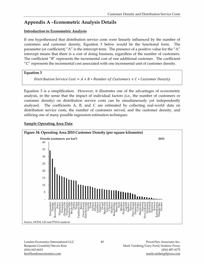
Customer Density and Distribution Service Costs
London Economics International LLC 49 PowerNex Associates Inc.
Benjamin Grunfeld/Steven Kim Mark Vainberg/Gary Ford/Andrew Poray
(416) 643-6610 (416) 487-4175
[email protected] [email protected]
Appendix A –Econometric Analysis Details
Introduction to Econometric Analysis
If one hypothesized that distribution service costs were linearly influenced by the number of
customers and customer density, Equation 3 below would be the functional form. The
parameter (or coefficient) “A” is the intercept term. The presence of a positive value for the “A”
intercept means that there is a cost of doing business, regardless of the number of customers.
The coefficient “B” represents the incremental cost of one additional customer. The coefficient
“C” represents the incremental cost associated with one incremental unit of customer density.
Equation 3
Equation 3 is a simplification. However, it illustrates one of the advantages of econometric
analysis, in the sense that the impact of individual factors (i.e., the number of customers or
customer density) on distribution service costs can be simultaneously yet independently
analyzed. The coefficients A, B, and C are estimated by collecting real-world data on
distribution service costs, the number of customers served, and the customer density, and
utilizing one of many possible regression estimation techniques.
Sample Operating Area Data
Figure 34: Operating Area 2010 Customer Density (per square kilometre)
Source: HONI; LEI and PNXA analysis
-
5
10
15
20
25
30
35
40
New
mark
etD
un
das
Bo
wm
an
vil
leE
sse
xW
inch
est
er
Kin
gst
on
Ora
ng
evil
leP
enet
an
gu
i…F
en
elo
n F
all
sB
rock
vil
leO
rill
iaP
icto
nV
an
kle
ek
Hil
lB
arr
ieO
wen
So
un
dP
eter
bo
rou
gh
Lin
coln
Pert
hA
ylm
erA
llis
ton
Lam
bto
nA
rnp
rio
rT
wee
dB
each
vil
leL
isto
wel
Cli
nto
nStr
ath
roy
Bra
ceb
rid
ge
Ban
cro
ftK
ent
Min
den
Wa
lke
rto
nG
uel
ph
Su
db
ury
Sim
coe
Parr
y S
ou
nd
Hu
nts
vil
leC
ob
den
Man
ito
uli
nA
lgo
ma
New
Lis
kea
rdN
ipis
sin
gK
irk
lan
d …
Tim
min
sK
en
ora
Kap
usk
asi
ng
Th
un
der
Bay
Dry
den
Density (customers per km2) 2010

Customer Density and Distribution Service Costs
London Economics International LLC 50 PowerNex Associates Inc.
Benjamin Grunfeld/Steven Kim Mark Vainberg/Gary Ford/Andrew Poray
(416) 643-6610 (416) 487-4175
[email protected] [email protected]
Figure 35: Operating Area 2010 Customer Density (per circuit kilometre)
Source: HONI; LEI and PNXA analysis
Figure 36: Operating Area 2010 OM&A Cost
Source: HONI; LEI and PNXA analysis
-
5
10
15
20
25
30
Du
nd
asN
ewm
ark
etL
inco
lnB
ow
man
vil
leT
imm
ins
Van
kle
ek H
ill
Kin
gst
on
Win
ches
ter
Bro
ckv
ille
Ori
llia
Arn
pri
or
Sud
bu
ryP
icto
nE
ssex
Fen
elo
n F
alls
Pen
etan
gu
is…
Bar
rie
Ow
en S
ou
nd
Tw
eed
Alg
om
aB
race
bri
dg
eP
eter
bo
rou
gh
Per
thK
irk
lan
d L
ake
Min
den
Sim
coe
Ora
ng
evil
leC
ob
den
Nip
issi
ng
Gu
elp
hL
amb
ton
All
isto
nH
un
tsv
ille
Ban
cro
ftL
isto
wel
Kap
usk
asin
gA
ylm
erP
arry
So
un
dC
lin
ton
Th
un
der
Bay
Wal
ker
ton
New
Lis
kea
rdB
each
vil
leM
anit
ou
lin
Stra
thro
yK
ent
Ken
ora
Dry
den
Density (customers per line-km) 2010
-
1
2
3
4
5
6
7
8
9
10
Tw
eed
Pet
erb
oro
ug
hP
erth
Ow
en S
ou
nd
Win
ches
ter
Th
un
der
Bay
Co
bd
enN
ewm
ark
etK
ing
sto
nB
ancr
oft
Bar
rie
Fen
elo
n F
alls
Hu
nts
vil
leE
ssex
Bra
ceb
rid
ge
Sud
bu
ryB
each
vil
leO
ran
gev
ille
Bro
ckv
ille
Nip
issi
ng
Par
ry S
ou
nd
Du
nd
asV
ank
leek
Hil
lM
ind
enW
alk
erto
nK
eno
raA
rnp
rio
rK
ent
Pic
ton
Cli
nto
nP
enet
ang
uis
hen
eB
ow
man
vil
leSi
mco
eO
rill
iaSt
rath
roy
Tim
min
sD
ryd
enL
amb
ton
Gu
elp
hA
ylm
erL
inco
lnN
ew L
isk
eard
Kap
usk
asin
gA
llis
ton
Man
ito
uli
nA
lgo
ma
Lis
tow
elK
irk
lan
d L
ake
Total Operating Area OM&A Cost (millions $) 2010

Customer Density and Distribution Service Costs
London Economics International LLC 51 PowerNex Associates Inc.
Benjamin Grunfeld/Steven Kim Mark Vainberg/Gary Ford/Andrew Poray
(416) 643-6610 (416) 487-4175
[email protected] [email protected]
Figure 37: Operating Area 2010 Capital Proxy
Source: HONI; LEI and PNXA analysis
-
2
4
6
8
10
12
14
16
18
Win
ches
ter
Tw
eed
Pet
erb
oro
ug
hN
ewm
ark
etB
arri
eP
erth
Ow
en S
ou
nd
Kin
gst
on
Fen
elo
n F
alls
Ora
ng
evil
leE
ssex
Th
un
der
Bay
Co
bd
enB
ancr
oft
Hu
nts
vil
leV
ank
leek
Hil
lB
race
bri
dg
eSu
db
ury
Wal
ker
ton
Ken
ora
Tim
min
sP
arry
So
un
dM
ind
enN
ipis
sin
gB
rock
vil
leB
ow
man
vil
leD
un
das
Arn
pri
or
Gu
elp
hB
each
vil
leA
llis
ton
Stra
thro
ySi
mco
eK
ent
Cli
nto
nP
icto
nD
ryd
enP
enet
ang
uis
hen
eL
amb
ton
Ori
llia
Man
ito
uli
nL
inco
lnA
ylm
erN
ew L
isk
eard
Alg
om
aK
irk
lan
d L
ake
Kap
usk
asin
gL
isto
wel
Total Operating Area Capital Cost (millions $) 2010

Customer Density and Distribution Service Costs
London Economics International LLC 52 PowerNex Associates Inc.
Benjamin Grunfeld/Steven Kim Mark Vainberg/Gary Ford/Andrew Poray
(416) 643-6610 (416) 487-4175
[email protected] [email protected]
Appendix B – Background Information on Distribution Systems
Distribution System Topology and Equipment
Electricity is typically generated at relatively low voltages, in the range of 20 to 25 kilovolts
(“kV”) in major generating stations and immediately transformed up to higher voltages (115
kV, 230 kV and 500 kV) for transmission to load centres.
Figure 38: Simplified Generation/Transmission/Distribution Model
Source: PNXA
Transmission substations transform the voltage back down to typically 44 kV for bulk
distribution of power via what are called sub-transmission or “M Class” feeders that supply
distribution stations. Distribution stations further transform the voltage down to typically 8 kV
for distribution feeder circuits that are used to supply customers. A simplified generation,
transmission, and distribution system model is illustrated in Figure 38.
The transformation process then continues one further step down to the 600, 230 or 115 volt
(“V”) level used in customers’ homes and businesses. This last transformation is done by pole-
top or pad-mounted transformers located relatively close to the customers, as illustrated in
Figure 39.

Customer Density and Distribution Service Costs
London Economics International LLC 53 PowerNex Associates Inc.
Benjamin Grunfeld/Steven Kim Mark Vainberg/Gary Ford/Andrew Poray
(416) 643-6610 (416) 487-4175
[email protected] [email protected]
Figure 39: Typical Single Phase Pole-Top Transformer
Source: PNXA files
The primary elements that make up a distribution system are the distribution feeders (lines or
cables), distribution stations, and metering and control systems. However, each of these
elements is comprised of many types of components. Overhead distribution lines, as illustrated
in Figure 39, include aluminum primary conductors, porcelain or polymeric line insulators,
fuses and fuse holders, pole-top transformers, secondary wiring, poles and pole hardware.
Underground and submarine cables are used sparingly because they are significantly more
costly than overhead lines. They include insulated primary cable, and pre-moulded
terminations and splices.
Distribution stations vary in design and complexity depending on their location and the
number of feeders connected by them. Figure 40 illustrates a typical open air distribution
station.

Customer Density and Distribution Service Costs
London Economics International LLC 54 PowerNex Associates Inc.
Benjamin Grunfeld/Steven Kim Mark Vainberg/Gary Ford/Andrew Poray
(416) 643-6610 (416) 487-4175
[email protected] [email protected]
Figure 40: Typical Open Air Distribution Station
Source: PNXA files
Stations of this type include transformers, circuit breakers and/or re-closers, disconnect
switches, grounding switches, bus conductors, protection, control and metering equipment,
station cables to facilitate line entrances and exits, and structural elements. In built-up areas
distribution stations may be enclosed in buildings or surrounded by improved appearance
walls and other aesthetic treatments.
Power quality standards require that the voltage and frequency be maintained within
prescribed limits. The frequency is controlled at the bulk transmission system level, however,
voltage control is a concern on distribution systems. Current flowing on long distribution
feeders causes a voltage drop along the feeder that is a function of loading. As well, loads with
lagging power factors (inductive loads for example, motors, air conditioners, etc.) require
reactive compensation in the form of capacitor banks which need to be switched in or out as
required. Voltage regulators, such as the single phase unit illustrated in Figure 41, are in
common use on long feeders to provide controlled voltage support when loads are high and
series inductors to limit voltage levels when loads are low.

Customer Density and Distribution Service Costs
London Economics International LLC 55 PowerNex Associates Inc.
Benjamin Grunfeld/Steven Kim Mark Vainberg/Gary Ford/Andrew Poray
(416) 643-6610 (416) 487-4175
[email protected] [email protected]
Figure 41: Single Phase Voltage Regulator (Left) and Three Phase Series Inductor (Right)
Source: PNXA files
Operation and Maintenance of Distribution Systems
Distribution infrastructure requires continual monitoring to ensure that the system is operating
normally and within the prescribed operational limits. Loadings need to be monitored to
ensure that currents and voltages are within equipment ratings, that loadings on the three
phases of feeders are balanced, and that opportunities for lowering system losses and
improving operational efficiencies are acted upon.
The condition of distribution station transformers needs to be monitored, circuit breakers and
re-closers include moving parts which wear out and need to be replaced, wood poles rot and
are attacked by insects and birds, and vegetation impinges on lines and needs to be removed or
trimmed for safety and reliability concerns. In addition, failures and weather related outages
occur, which require immediate action to repair because many cause customers to be without
power for a period of time. The extent of operational maintenance and repair is influenced by
the age of the infrastructure, the environment in the location in the province, and the geography
of the location (e.g., heavily forested versus farm land). This latter factor also influences the
topology of the system which affects work methods and accessibility.
The topology of distribution systems can vary considerably which may impact distribution
operating and sustainment costs. Figure 42 is a snapshot view from HONI’s GIS showing one
of the distribution stations in the Bracebridge operating area and a number of feeders supplied
from that distribution station, as well as the location of the transformers supplying customers
on the feeders.

Customer Density and Distribution Service Costs
London Economics International LLC 56 PowerNex Associates Inc.
Benjamin Grunfeld/Steven Kim Mark Vainberg/Gary Ford/Andrew Poray
(416) 643-6610 (416) 487-4175
[email protected] [email protected]
Figure 42: Typical Radial Feeder Topology in Northern Ontario
Notes: Feeders are shown as lines, triangles represent transformers feeding customers, and the purple rectangle indicates the distribution station Source: HONI
In contrast, Figure 43 illustrates a typical feeder topology from the Simcoe operating area in
southern Ontario. While both of these distribution systems are operated “radially” from the
distribution stations, the grid-like regularity of the system in Simcoe offers opportunities for
multiple interconnections of feeders, which in turn provides increased flexibility and
operational reliability.36 If the number of customers in a given area is large enough, most
distribution utilities use a meshed system design (as shown in Figure 43) to reduce the number
of customers affected by an outage and improve the reliability of supply.
36 A radial network consists of a series of “spokes” and “hubs”. Distribution feeders leave a DS and pass through
the network area with no normal connection to any other supply. This is typical of long rural lines with isolated load areas. An interconnected or “mesh” network is generally found in more urban areas and will have multiple connections to other points of supply. These points of connection are normally open but allow for various configurations through the opening and closing of switches.

Customer Density and Distribution Service Costs
London Economics International LLC 57 PowerNex Associates Inc.
Benjamin Grunfeld/Steven Kim Mark Vainberg/Gary Ford/Andrew Poray
(416) 643-6610 (416) 487-4175
[email protected] [email protected]
Figure 43: Grid-like Feeder Topology Typical in Southern Ontario
Notes: Feeders are shown as lines, triangles represent transformers feeding customers, and the blue rectangle indicates the distribution station Source: HONI
In addition, feeders in the heavily forested and rocky areas may have greater off-road lengths,
as illustrated in Figure 44, and require more rock and crib pole mounts, which are generally
more difficult and costly to access and maintain.
Figure 44: Typical Off Road Rights of Way
Source: PNXA files

Customer Density and Distribution Service Costs
London Economics International LLC 58 PowerNex Associates Inc.
Benjamin Grunfeld/Steven Kim Mark Vainberg/Gary Ford/Andrew Poray
(416) 643-6610 (416) 487-4175
[email protected] [email protected]
Appendix C – Direct Cost Assignment Analysis Details
Sample Area Maps
Figure 45: Bracebridge Operating Area Map
Source: HONI

Customer Density and Distribution Service Costs
London Economics International LLC 59 PowerNex Associates Inc.
Benjamin Grunfeld/Steven Kim Mark Vainberg/Gary Ford/Andrew Poray
(416) 643-6610 (416) 487-4175
[email protected] [email protected]
Figure 46: Dryden Operating Area Map
Source: HONI

Customer Density and Distribution Service Costs
London Economics International LLC 60 PowerNex Associates Inc.
Benjamin Grunfeld/Steven Kim Mark Vainberg/Gary Ford/Andrew Poray
(416) 643-6610 (416) 487-4175
[email protected] [email protected]
Figure 47: Essex Operating Area Map
Source: HONI

Customer Density and Distribution Service Costs
London Economics International LLC 61 PowerNex Associates Inc.
Benjamin Grunfeld/Steven Kim Mark Vainberg/Gary Ford/Andrew Poray
(416) 643-6610 (416) 487-4175
[email protected] [email protected]
Figure 48: Kingston Operating Area Map
Source: HONI

Customer Density and Distribution Service Costs
London Economics International LLC 62 PowerNex Associates Inc.
Benjamin Grunfeld/Steven Kim Mark Vainberg/Gary Ford/Andrew Poray
(416) 643-6610 (416) 487-4175
[email protected] [email protected]
Figure 49: Newmarket Operating Area Map
Source: HONI
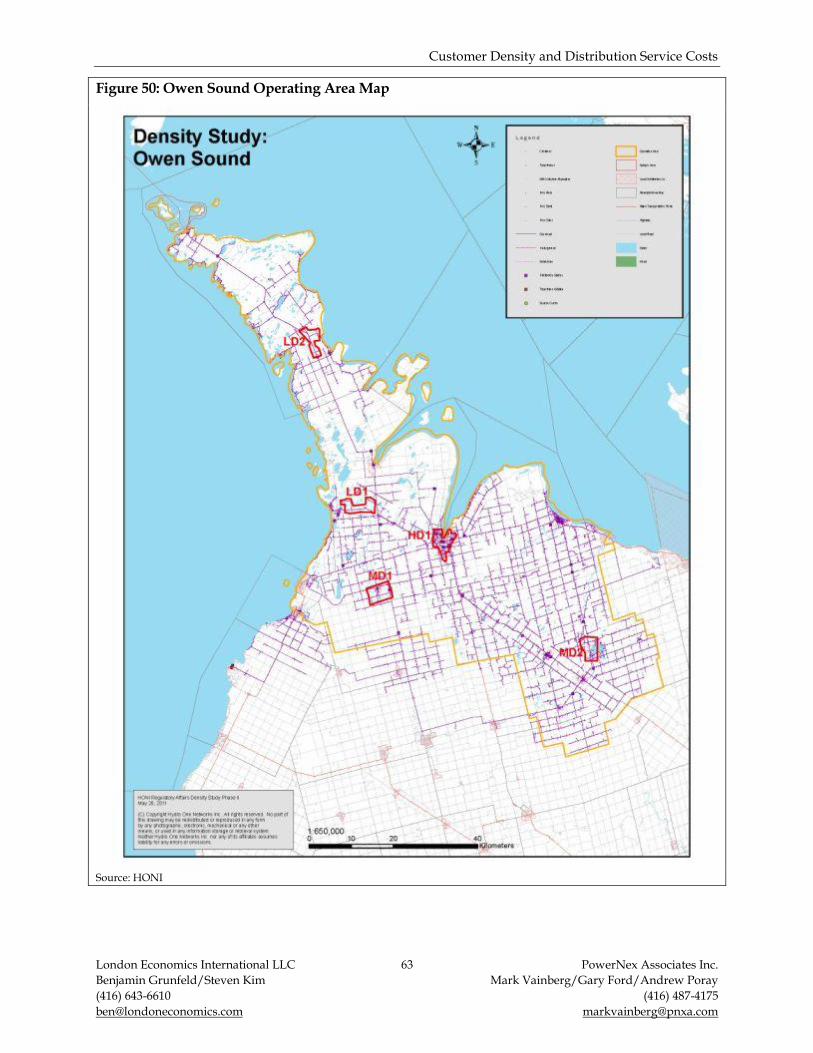
Customer Density and Distribution Service Costs
London Economics International LLC 63 PowerNex Associates Inc.
Benjamin Grunfeld/Steven Kim Mark Vainberg/Gary Ford/Andrew Poray
(416) 643-6610 (416) 487-4175
[email protected] [email protected]
Figure 50: Owen Sound Operating Area Map
Source: HONI

Customer Density and Distribution Service Costs
London Economics International LLC 64 PowerNex Associates Inc.
Benjamin Grunfeld/Steven Kim Mark Vainberg/Gary Ford/Andrew Poray
(416) 643-6610 (416) 487-4175
[email protected] [email protected]
Figure 51: Perth Operating Area Map
Source: HONI

Customer Density and Distribution Service Costs
London Economics International LLC 65 PowerNex Associates Inc.
Benjamin Grunfeld/Steven Kim Mark Vainberg/Gary Ford/Andrew Poray
(416) 643-6610 (416) 487-4175
[email protected] [email protected]
Figure 52: Peterborough Operating Area Map
Source: HONI

Customer Density and Distribution Service Costs
London Economics International LLC 66 PowerNex Associates Inc.
Benjamin Grunfeld/Steven Kim Mark Vainberg/Gary Ford/Andrew Poray
(416) 643-6610 (416) 487-4175
[email protected] [email protected]
Figure 53: Simcoe Operating Area Map
Source: HONI

Customer Density and Distribution Service Costs
London Economics International LLC 67 PowerNex Associates Inc.
Benjamin Grunfeld/Steven Kim Mark Vainberg/Gary Ford/Andrew Poray
(416) 643-6610 (416) 487-4175
[email protected] [email protected]
Figure 54: Sudbury Operating Area Map
Source: HONI
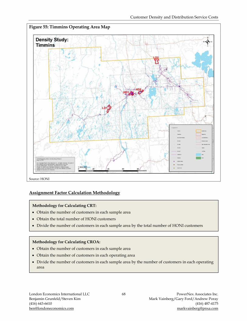
Customer Density and Distribution Service Costs
London Economics International LLC 68 PowerNex Associates Inc.
Benjamin Grunfeld/Steven Kim Mark Vainberg/Gary Ford/Andrew Poray
(416) 643-6610 (416) 487-4175
[email protected] [email protected]
Figure 55: Timmins Operating Area Map
Source: HONI
Assignment Factor Calculation Methodology
Methodology for Calculating CROA:
Obtain the number of customers in each sample area
Obtain the number of customers in each operating area
Divide the number of customers in each sample area by the number of customers in each operating
area
Methodology for Calculating CRT:
Obtain the number of customers in each sample area
Obtain the total number of HONI customers
Divide the number of customers in each sample area by the total number of HONI customers

Customer Density and Distribution Service Costs
London Economics International LLC 69 PowerNex Associates Inc.
Benjamin Grunfeld/Steven Kim Mark Vainberg/Gary Ford/Andrew Poray
(416) 643-6610 (416) 487-4175
[email protected] [email protected]
Methodology for Calculating IRS:
Calculate the total length of the distribution feeders that traverse a sample area
Calculate the total length within the sample area of the distribution feeders that traverse the sample
area
Calculate the total number of storm related interruptions and non-interruptions associated with all
of the distribution feeders that traverse a sample area
Divide the total length of distribution feeders within the sample area by the total length of the
feeders that traverse the sample area
Multiply this ratio by the number of storm related interruptions and non-interruptions associated
with the feeders
Methodology for Calculating IRNS:
Calculate the total length of the distribution feeders that traverse a sample area
Calculate the total length within the sample area of the distribution feeders that traverse the sample
area
Calculate the total number of non-storm related interruptions and non-interruptions associated
with all of the distribution feeders that traverse a sample area
Divide the total length of distribution feeders within the sample area by the total length of the
feeders that traverse the sample area
Multiply this ratio by the number of non-storm related interruptions and non-interruptions
associated with the feeders
Methodology for Calculating PDRT:
Calculate the total (aggregate) distance from each pole in a sample area to the closest service center
Calculate the total (aggregate) distance from each pole in an operating area to the closest service
center
Divide the sample area total pole distance by the operating area total pole distance
Methodology for Calculating UGR:
Calculate the total length of underground conductor in a sample area
Calculate the total length of underground conductor in an operating area
Divide the sample area total length by the operating area total length
Methodology for Calculating CDR:
Calculate the total (aggregate) distance from each customer in a sample area to the closest service
center
Calculate the total (aggregate ) distance from each customer in an operating area to the closest
service center
Divide the sample area total distance by the operating area total distance

Customer Density and Distribution Service Costs
London Economics International LLC 70 PowerNex Associates Inc.
Benjamin Grunfeld/Steven Kim Mark Vainberg/Gary Ford/Andrew Poray
(416) 643-6610 (416) 487-4175
[email protected] [email protected]
Individual Sample Area Assignment Factors
Figure 56: Individual Sample Area Assignment Factors (2010)
Source: LEI and PNXA analysis
Operating Area Sample Area CRT CROA CDR UGR PDRT IRNS IRS
Bracebridge LD1 0.000 0.008 0.014 0.009 0.018 0.017 0.018
Bracebridge LD2 0.000 0.005 0.003 0.011 0.007 0.013 0.030
Bracebridge LD3 0.000 0.006 0.004 0.011 0.008 0.008 0.002
Bracebridge MD1 0.001 0.058 0.061 0.077 0.044 0.048 0.065
Bracebridge MD2 0.001 0.073 0.087 0.002 0.062 0.069 0.051
Bracebridge MD3 0.001 0.038 0.033 0.023 0.032 0.043 0.043
Dryden LD1 0.000 0.008 0.009 0.000 0.014 0.012 0.000
Dryden LD2 0.000 0.002 0.004 0.000 0.024 0.028 0.000
Dryden MD1 0.001 0.071 0.113 0.033 0.036 0.026 0.000
Dryden MD2 0.001 0.086 0.217 0.030 0.092 0.073 0.000
Dryden HD1 0.003 0.295 0.014 0.364 0.004 0.105 0.000
Essex LD1 0.000 0.005 0.003 0.000 0.007 0.009 0.002
Essex LD2 0.000 0.005 0.006 0.000 0.014 0.022 0.016
Essex MD1 0.001 0.026 0.045 0.016 0.031 0.026 0.045
Essex MD2 0.001 0.027 0.021 0.020 0.020 0.015 0.003
Essex HD1 0.002 0.066 0.072 0.079 0.034 0.042 0.077
Essex HD2 0.002 0.058 0.075 0.147 0.034 0.028 0.021
Kingston LD1 0.000 0.002 0.003 0.000 0.013 0.012 0.011
Kingston LD2 0.000 0.002 0.004 0.000 0.013 0.014 0.022
Kingston MD1 0.001 0.014 0.009 0.001 0.009 0.008 0.001
Kingston MD2 0.001 0.018 0.015 0.008 0.015 0.014 0.028
Kingston HD1 0.009 0.233 0.050 0.295 0.010 0.120 0.057
Newmarket LD1 0.000 0.005 0.007 0.002 0.021 0.000 0.000
Newmarket LD2 0.000 0.005 0.006 0.006 0.012 0.000 0.000
Newmarket LD3 0.000 0.003 0.001 0.006 0.002 0.008 0.000
Newmarket MD1 0.001 0.018 0.007 0.039 0.006 0.019 0.000
Newmarket HD1 0.003 0.072 0.115 0.009 0.102 0.081 0.000
Newmarket HD2 0.007 0.180 0.187 0.106 0.024 0.094 0.000
Newmarket HD3 0.007 0.170 0.164 0.166 0.017 0.092 0.000
Newmarket HD4 0.003 0.078 0.031 0.078 0.015 0.023 0.000
Owen Sound LD1 0.000 0.002 0.002 0.013 0.004 0.002 0.000
Owen Sound LD2 0.000 0.001 0.000 0.000 0.008 0.003 0.016
Owen Sound MD1 0.000 0.013 0.013 0.015 0.008 0.022 0.001
Owen Sound MD2 0.000 0.011 0.023 0.004 0.019 0.015 0.016
Owen Sound HD1 0.008 0.215 0.022 0.090 0.003 0.082 0.018
Perth LD1 0.000 0.002 0.001 0.000 0.003 0.006 0.002
Perth LD2 0.000 0.003 0.002 0.008 0.004 0.006 0.019
Perth MD1 0.001 0.021 0.008 0.034 0.006 0.019 0.017
Perth MD2 0.000 0.014 0.020 0.010 0.017 0.012 0.008
Perth HD1 0.003 0.098 0.007 0.202 0.002 0.054 0.000
Perth HD2 0.004 0.138 0.129 0.063 0.040 0.085 0.002
Peterborough LD1 0.000 0.003 0.004 0.000 0.008 0.008 0.000
Peterborough LD2 0.000 0.004 0.002 0.000 0.003 0.011 0.000
Peterborough MD1 0.001 0.025 0.024 0.018 0.011 0.016 0.000
Peterborough MD2 0.001 0.031 0.027 0.048 0.011 0.016 0.000
Peterborough MD3 0.001 0.032 0.009 0.003 0.017 0.023 0.000
Simcoe LD1 0.000 0.010 0.014 0.006 0.016 0.008 0.000
Simcoe LD2 0.000 0.008 0.013 0.001 0.022 0.023 0.011
Simcoe MD1 0.001 0.060 0.068 0.090 0.040 0.008 0.006
Simcoe MD2 0.001 0.060 0.083 0.075 0.022 0.012 0.021
Simcoe MD3 0.000 0.029 0.015 0.001 0.009 0.000 0.000
Sudbury LD1 0.000 0.004 0.007 0.004 0.025 0.021 0.037
Sudbury LD2 0.000 0.003 0.002 0.004 0.008 0.009 0.009
Sudbury MD1 0.001 0.028 0.037 0.010 0.042 0.021 0.012
Sudbury MD2 0.001 0.024 0.013 0.003 0.017 0.019 0.007
Sudbury HD1 0.004 0.138 0.081 0.187 0.036 0.079 0.017
Sudbury HD2 0.003 0.099 0.089 0.061 0.046 0.068 0.021
Sudbury HD3 0.002 0.060 0.000 0.047 0.027 0.042 0.011
Timmins LD1 0.000 0.005 0.014 0.000 0.014 0.015 0.051
Timmins LD2 0.000 0.002 0.006 0.003 0.025 0.011 0.033
Timmins HD1 0.011 0.580 0.115 0.723 0.015 0.342 0.098
Timmins HD2 0.002 0.132 0.101 0.102 0.024 0.085 0.047

Customer Density and Distribution Service Costs
London Economics International LLC 71 PowerNex Associates Inc.
Benjamin Grunfeld/Steven Kim Mark Vainberg/Gary Ford/Andrew Poray
(416) 643-6610 (416) 487-4175
[email protected] [email protected]
Individual Sample Area Results
Figure 57: Low-Density Sample Area Results
Source: LEI and PNXA analysis
Operating Area Sample Area OM&A Asset Intensity
Bracebridge LD1 277 23,817
Dryden LD1 218 34,896
Essex LD1 89 25,687
Kingston LD1 346 12,548
Newmarket LD1 155 23,732
Owen Sound LD1 216 27,692
Perth LD1 340 33,480
Peterborough LD1 266 28,154
Simcoe LD1 173 25,271
Sudbury LD1 254 7,083
Timmins LD1 245 24,733
Bracebridge LD2 809 15,450
Dryden LD2 1,868 45,610
Essex LD2 228 27,043
Kingston LD2 412 33,199
Newmarket LD2 151 16,330
Owen Sound LD2 307 33,400
Perth LD2 401 21,384
Peterborough LD2 222 26,749
Simcoe LD2 425 34,298
Sudbury LD2 656 33,591
Timmins LD2 348 61,279
Bracebridge LD3 524 32,374
Newmarket LD3 170 22,397
379 27,925Average

Customer Density and Distribution Service Costs
London Economics International LLC 72 PowerNex Associates Inc.
Benjamin Grunfeld/Steven Kim Mark Vainberg/Gary Ford/Andrew Poray
(416) 643-6610 (416) 487-4175
[email protected] [email protected]
Figure 58: Medium-Density Sample Area Results
Source: LEI and PNXA analysis
Operating Area Sample Area Asset Intensity
Bracebridge MD1 342 13,601
Dryden MD1 164 9,745
Essex MD1 156 7,668
Kingston MD1 83 9,493
Newmarket MD1 111 8,707
Owen Sound MD1 114 11,041
Perth MD1 141 11,689
Peterborough MD1 166 13,689
Simcoe MD1 147 8,848
Sudbury MD1 158 8,873
Bracebridge MD2 165 18,338
Dryden MD2 219 11,723
Essex MD2 99 9,206
Kingston MD2 103 7,353
Owen Sound MD2 219 15,228
Perth MD2 212 14,903
Peterborough MD2 153 9,910
Simcoe MD2 135 4,848
Sudbury MD2 122 10,259
Bracebridge MD3 150 13,232
Peterborough MD3 103 6,950
Simcoe MD3 168 12,113
156 10,792Average

Customer Density and Distribution Service Costs
London Economics International LLC 73 PowerNex Associates Inc.
Benjamin Grunfeld/Steven Kim Mark Vainberg/Gary Ford/Andrew Poray
(416) 643-6610 (416) 487-4175
[email protected] [email protected]
Figure 59: High-Density Sample Area Results
Source: LEI and PNXA analysis
Additional Scatter Plots
Figure 60: Relationship between OM&A Costs and Customer Density (per circuit kilometre)
Source: LEI and PNXA analysis
Operating Area Sample Area OM&A Asset Intensity
Dryden HD1 77 8,323
Essex HD1 126 5,076
Kingston HD1 57 2,882
Newmarket HD1 130 9,037
Owen Sound HD1 58 4,700
Perth HD1 76 7,740
Sudbury HD1 77 4,631
Timmins HD1 69 2,709
Essex HD2 157 4,451
Newmarket HD2 87 3,773
Perth HD2 113 7,136
Sudbury HD2 90 4,946
Timmins HD2 91 4,905
Newmarket HD3 91 2,265
Sudbury HD3 56 6,176
Newmarket HD4 75 5,151
89 5,244Average
-
200
400
600
800
1,000
1,200
1,400
1,600
1,800
2,000
0 20 40 60 80 100
OM
&A
Co
st
($)
per
Cu
sto
mer
Customers per Circuit KilometreLD MD HD

Customer Density and Distribution Service Costs
London Economics International LLC 74 PowerNex Associates Inc.
Benjamin Grunfeld/Steven Kim Mark Vainberg/Gary Ford/Andrew Poray
(416) 643-6610 (416) 487-4175
[email protected] [email protected]
Figure 61: Relationship between Asset Intensity and Customer Density (per circuit kilometre)
Source: LEI and PNXA analysis
Estimated Density of Existing Rate Classes
The following figures are based on data provided by HONI from the GIS. A grid consisting of
one square kilometre cells was layered over the 11 operating areas included in the direct cost
assignment analysis. The number of customers within an individual grid cell is equal to the
density of the grid cell. Figure 62 through Figure 67 plot the probability and cumulative
distributions of customer density for HONI’s existing UR, R1, R2, Seasonal, Urban General
Service (UGe and UGd), and General Service (GSe and GSd) rate classes, respectively.
Figure 62: Customer Density Distribution for HONI’s UR Rate Class in 11 Operating Areas
Source: HONI; LEI and PNXA analysis
-
10,000
20,000
30,000
40,000
50,000
60,000
70,000
0 20 40 60 80 100
Asset
Rep
lacem
en
t C
ost
($)
per
Cu
sto
mer
Customers per Circuit KilometreLD MD HD
0%
100%
0%
1%
2%
3%
4%
5%
0-1
0
10
0-1
10
20
0-2
10
30
0-3
10
40
0-4
10
50
0-5
10
60
0-6
10
70
0-7
10
80
0-8
10
90
0-9
10
10
00
-1
01
0
11
00
-1
11
0
12
00
-1
21
0
13
00
-1
31
0
14
00
-1
41
0
15
00
-1
51
0
16
00
-1
61
0
17
00
-1
71
0
18
00
-1
81
0
19
00
-1
91
0
20
00
-2
01
0
Customer Density (per Square Kilometre)
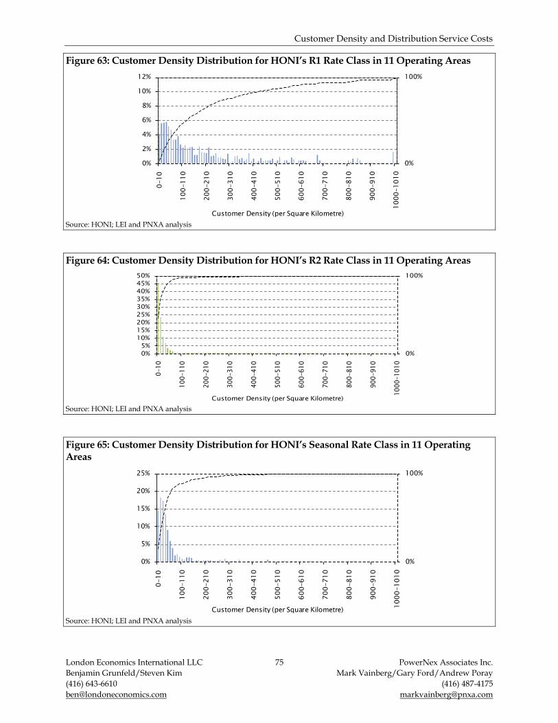
Customer Density and Distribution Service Costs
London Economics International LLC 75 PowerNex Associates Inc.
Benjamin Grunfeld/Steven Kim Mark Vainberg/Gary Ford/Andrew Poray
(416) 643-6610 (416) 487-4175
[email protected] [email protected]
Figure 63: Customer Density Distribution for HONI’s R1 Rate Class in 11 Operating Areas
Source: HONI; LEI and PNXA analysis
Figure 64: Customer Density Distribution for HONI’s R2 Rate Class in 11 Operating Areas
Source: HONI; LEI and PNXA analysis
Figure 65: Customer Density Distribution for HONI’s Seasonal Rate Class in 11 Operating Areas
Source: HONI; LEI and PNXA analysis
0%
100%
0%
2%
4%
6%
8%
10%
12%
0-1
0
10
0-1
10
20
0-2
10
30
0-3
10
40
0-4
10
50
0-5
10
60
0-6
10
70
0-7
10
80
0-8
10
90
0-9
10
10
00
-1
01
0
Customer Density (per Square Kilometre)
0%
100%
0%
5%
10%
15%
20%
25%
30%
35%
40%
45%
50%
0-1
0
10
0-1
10
20
0-2
10
30
0-3
10
40
0-4
10
50
0-5
10
60
0-6
10
70
0-7
10
80
0-8
10
90
0-9
10
10
00
-1
01
0Customer Density (per Square Kilometre)
0%
100%
0%
5%
10%
15%
20%
25%
0-1
0
10
0-1
10
20
0-2
10
30
0-3
10
40
0-4
10
50
0-5
10
60
0-6
10
70
0-7
10
80
0-8
10
90
0-9
10
10
00
-1
01
0
Customer Density (per Square Kilometre)

Customer Density and Distribution Service Costs
London Economics International LLC 76 PowerNex Associates Inc.
Benjamin Grunfeld/Steven Kim Mark Vainberg/Gary Ford/Andrew Poray
(416) 643-6610 (416) 487-4175
[email protected] [email protected]
Figure 66: Customer Density Distribution for HONI’s UGe and UGd Rate Classes in 11 Operating Areas
Source: HONI; LEI and PNXA analysis
Figure 67: Customer Density Distribution for HONI’s GSe and GSd Rate Classes in 11 Operating Areas
Source: HONI; LEI and PNXA analysis
0%
100%
0%
5%
10%
15%
20%
25%
0-1
0
10
0-1
10
20
0-2
10
30
0-3
10
40
0-4
10
50
0-5
10
60
0-6
10
70
0-7
10
80
0-8
10
90
0-9
10
10
00
-1
01
0
11
00
-1
11
0
12
00
-1
21
0
13
00
-1
31
0
14
00
-1
41
0
15
00
-1
51
0
16
00
-1
61
0
17
00
-1
71
0
18
00
-1
81
0
19
00
-1
91
0
20
00
-2
01
0
Customer Density (per Square Kilometre)
0%
100%
0%
5%
10%
15%
20%
25%
0-1
0
10
0-1
10
20
0-2
10
30
0-3
10
40
0-4
10
50
0-5
10
60
0-6
10
70
0-7
10
80
0-8
10
90
0-9
10
10
00
-1
01
0
Customer Density (per Square Kilometre)


Benjamin Grunfeld Associate Director
Navigant Bay Adelaide Centre 333 Bay Street, Suite 1250 Toronto, ON M5H 2R2 Tel: +1 (416) 777-2444 Fax: +1 (416) 777-2441 Cell: +1 (647) 960-3632 [email protected]
Professional History • London Economics International;
Managing Consultant; Toronto, Canada
• Ampersand Energy Partners; Senior Associate; Boston, USA
• Navigant; Senior Consultant; Toronto, Canada
• Hatch; Junior Engineer; Mississauga, Canada
Education • M.Sc. Management and Economics;
London School of Economics and Political Science; London, UK; 2008-2009
• B.Sc. Applied Mathematics and Electrical Engineering; Queen’s University; Kingston, Canada; 1998-2003
Benjamin Grunfeld
Benjamin Grunfeld is an Associate Director in the Energy Practice at Navigant.
Benjamin provides strategic advice and analytical expertise to utilities, independent power producers, independent transmission companies, energy-related business ventures, governments, and arm’s-length government agencies. He has considerable experience in the areas of energy policy design, power procurement, generation and transmission project development and finance, electricity market analysis and price forecasting, and utility regulatory economics. Benjamin has worked in regulated and deregulated markets across North America, as well as a range of developed and emerging economies around the world. He is responsible for all aspects of project fulfillment.
Prior to joining Navigant, Benjamin worked for London Economics International, a global economic, financial, and strategic advisory professional services firm, which specializes in energy, water, and infrastructure. He started his career as an engineer in the power and electro-technology group at Hatch.
Professional Experience
Transmission, Distribution, and Retail
» Technical advisor to Ontario Distribution Sector Review Panel – Provided technical consulting services to the Ontario Ministry of Energy in support of the Ontario Distribution Sector Review Panel. As part of this engagement, Benjamin managed a team providing insight on previous distributor mergers and quantification of associated savings, trends in distributor spending and implications on the potential for further efficiencies, cost drivers for LDCs and potential efficiencies, and areas where distributors are currently sharing common infrastructure, systems, and processes, and the potential for further efficiencies in these areas. [Client: Ontario Ministry of Energy; Date: 2012; Location: Ontario, Canada]

Benjamin Grunfeld
Page 2
» Customer density and cost allocation study – Benjamin and his team were engaged by Hydro One Networks, Inc. to review the existing density-based rate class design and cost allocation mechanisms associated with the utility’s electricity distribution business. The objective of the study is to establish a set of well-defined and defendable customer classes that take into account appropriate density differentiation. Benjamin led a consortium of firms providing econometric, engineering, and strategic advice to Hydro One Networks, Inc. in order to complete the study and assist with preparations for an upcoming rate application. Benjamin led two stakeholder engagement sessions. The first, to garner input into the methodology development, and the second, following the completion of the study, to present the results and findings. [Client: Hydro One Networks, Inc.; Date: 2011; Location: Ontario, Canada]
» Due diligence support for potential investment in merchant transmission project - Prepared three detailed presentations analyzing four proposed merchant high-voltage direct current transmission projects in the US. Analysis includes detailing the development roadmap and the current status of the proposed projects, identifying potential competitive threats from other similar competing transmission lines and local generation, and examining the renewable needs and willingness to pay of utilities on either end of the proposed transmission line. [Client: Confidential (Independent Transmission Company); Date: 2011; Location: Multiple, USA]
» Drafting private placement memorandum for merchant transmission developer - Drafted a private placement memorandum for a merchant transmission developer’s Series B capital raise. Responded to investor queries in relation to market value of transmission services, financing arrangements, and competitive threats. [Client: Confidential (Independent Transmission Company); Date: 2011; Location: Multiple, USA]
» Merchant transmission asset valuation and project development support - Benjamin was the lead financial and market advisor to a US merchant transmission company developing to value a three-way high voltage direct current connection between the Eastern, Western, and Texas interconnections in the United States. Ben led a team to project energy prices in the markets surrounding the proposed project, including the Southwest Power Pool, the Western Electricity Coordinating Council, and the Electric Reliability Council of Texas regional markets. Ben was responsible for developing revenue forecasts for the project over a 20-year period; the project is subject to market-based rates. Ben also advising on other financing, regulatory, and development related issues. [Client: Confidential (Independent Transmission Company); Date: 2010; Location: Multiple, USA]
» Analysis of competition in the Texas retail electricity market - Prepared a white paper on competition in the Texas residential and commercial retail electricity market. Provided an overview of the structure of the retail electricity market (history, size, suppliers, elasticity of demand and customer switching), performed market share and Herfindahl-Hirschman Index analysis and evaluated the potential impact of a proposed merger. [Client: Confidential (Retail Electricity Provider); Date: 2010; Location: Texas, USA]
» Electricity distribution tariff design - Provided advisory support to the Electricity and Cogeneration Regulatory Authority for the Kingdom of Saudi Arabia. Ben assisted in the development of a long-term electricity tariff model and framework designed to achieve revenue sufficiency for the electricity sector as a whole for several regulatory periods from 2008 onwards. The tariff design embedded efficiency targets and incorporated a lifeline tariff for residential customers amongst other features. [Client: Electricity and Cogeneration Regulatory Authority; Date: 2007-2008; Location: Saudi Arabia]
» Benchmarking of distribution utility customer care costs - Part of a team that provided an independent assessment of the competitiveness of pricing for customer care services. Ben analyzed and assessed the relative complexity of retail and regulated market structures in the United States

Benjamin Grunfeld
Page 3
and Canada, and prepared an overview of service quality requirements in multiple jurisdictions relative requirements in master service agreement. In addition, Ben also provided a benchmarking analysis of United States and Canadian electricity and gas utility customer care related costs. [Client: Confidential (Utility); Date: 2006; Location: Alberta, Canada]
» Retail electricity supply market-entry strategy - Led the development of a long-term wholesale electricity price forecast and market assessment report. Formulated and presented a market-entry and project-development strategy. [Client: Confidential (Retail Electricity Provider); Date: 2005; Location: Ontario, Canada]
Multi-Segment
» Industrial Energy Initiative program design – Advised both the Ontario Power Authority and the Ontario Ministry of Energy on the development of the Industrial Energy Initiative (IEI), which effectively offers new and existing industrial load in the province premium rates for electricity. Advised on a number of program design issues including: appropriate tariff levels, the impact on other customer classes, eligibility criteria, and the role of energy efficiency, among other issues. [Ontario Power Authority; Date: 2012; Location: Ontario, Canada]
» Forecast of Ontario wholesale and consumer electricity prices – Benjamin led a team of three consultants providing a quarterly forecast of wholesale and consumer electricity prices to a retail electric provider with generation assets in Ontario. Analysis included a monthly five-year forecast of the Hourly Ontario Electricity Price (“HOEP”) and the Global Adjustment (“GA”). [Client: Confidential (Retail Electricity Provider); Date: 2011; Location: Ontario, Canada]
» Review of the Ontario market structure and recommendations for improvement - Authored a report on the current electricity market structure in Ontario and develop a series of recommendations aimed at lowering the overall cost of electricity supply to consumers and improving the sector’s effectiveness. Led a team of consultants analyzing three key issues: the rising cost of electricity supply; the imbalance in the supply mix, both in terms of the overall installed generation capacity and the relative proportion of baseload and intermittent resources; and the distortion of the wholesale market price signal. [Client: Direct Energy Marketing, Ltd.; Date: 2011; Location: Ontario, Canada]
» Comprehensive assessment of the British Columbia power sector - Ben and his team developed a comprehensive report outlining the dynamics of the British Columbia electricity sector, in particular on Vancouver Island. The report analyzed long-term supply demand dynamics as well as the evolution of the Province’s transmission network. The report also incorporated a synopsis of the recently introduced green energy legislation and its potential impact on the sector. [Client: Confidential (Independent Power Producer); Date: 2010; Location: British Columbia, Canada]
» Analyzing the cost of the Ontario Green Energy Act, 2009 - Led a team that developed a comprehensive independent analysis of the potential cost associated with the Ontario Green Energy Act, 2009. The analysis included estimates of the cost to Ontarians of: generation procured under a renewable energy feed-in tariff program; interconnection of new renewable facilities; the development and implementation of a “smart grid”; and new conservation and demand management initiatives. The engagement also required Ben to respond to media requests and facilitate a media conference. [Client: Official Opposition in Ontario; Date: 2009; Location: Ontario, Canada]
» New England wholesale and capacity price forecasting and market analysis - Developed 20-year forecasts of wholesale electricity and capacity market prices in the Independent System Operator New England control region. The work supported the successful re-financing of two hydro-electric

Benjamin Grunfeld
Page 4
facilities, one run-of-river and one pumped storage. [Client: Confidential (Independent Power Producer); Date: 2007; Location: New England, USA]
» Ontario wholesale and consumer price forecasting and market analysis - Led the development of a long-term wholesale and consumer electricity price forecast and market assessment report. The report addressed the impact of supply-side announcements, including the Minister of Energy’s Supply Mix Directive to the Ontario Power Authority. The study also discussed the impact of the delay in the retirement of Ontario’s coal-fired capacity. [Client: Exxon Mobil; Date: 2006; Location: Ontario, Canada]
» Integrated resource plan development support - Led the development of a peak demand forecast for the Ontario Power Authority’s Integrated Power System Plan. Tasks included: estimating the impacts of various conservation and demand management scenarios; developing an hourly forecast of energy and peak demand; estimating end-use contributions to peak demand; estimating potential conservation and demand management impacts, by end-use; developing weather normalization algorithms and methodologies to weather-correct/normalize historic load data; estimating the impact of a system-wide deployment of time-of-use meters and time-of-use pricing on Ontario demand. [Client: Ontario Power Authority; Date: 2006; Location: Ontario, Canada]
» Ontario wholesale and consumer price forecasting and market analysis - One of the primary authors of Navigant’s semi-annual Ontario Market Assessment multi-client study. The assessment contains a detailed overview of the Ontario market, past and present. It includes an analysis of the implications of recent market developments and an outlook onto future developments. The report also contains a wholesale market price forecast and an in-depth analysis of the effective consumer (or blended consumer) price. As a major contributor to multiple Ontario Market Assessments, Ben authored multiple sections of the report and performed the detailed analysis that accompanies the assessment; developed the fuel cost, demand and supply forecasts, and many other forecast assumptions underpinning the wholesale market price forecast. Ben also developed the estimate of the blended consumer price including an estimate of the “Global Adjustment”. [Client: Multiple; Date: 2004-2006; Location: Ontario, Canada]
» Variance tracking for Ontario regulated price plan - Responsible for tracking and interpreting the variance between the forecast and actual Regulated Price Plan supply costs. Developed numerous summary and explanatory documents for both internal and public consumption. Developed the template for the “Monthly Variance Explanation” document posted monthly to Ontario Energy Board website. [Client: Ontario Energy Board; Date: 2005-2006; Location: Ontario, Canada]
» Integrated resource plan development support - Performed analysis and provided support during the development of the Ontario Supply Mix Advice. Aided in the preparation and delivery of a seminar on modeling alternatives for portfolio analysis, highlighting available tools and resources. Developed an Excel based model to quantify portfolio costs and risks for the Ontario Power Authority’s report to the Ministry of Energy on the long term supply of electricity generation resources. Additional tasks included: developing a model to assess the peak demand impacts of conservation and time-of-use initiatives: developing conservation and smart meter load profile decrements for use within the portfolio evaluation model; developing a method for modeling weather impacts on base demand and conservation decrements. [Client: Ontario Power Authority; Date: 2005-2006; Location: Ontario, Canada]
» Regional wholesale and consumer price forecasting and market analysis - Led the development of a comprehensive assessment of the Ontario, Michigan, New York and Quebec electricity markets. The assessment included a Political-Economic-Socio-cultural-Technological analysis for Ontario and the neighbouring markets combined. The report provided a long-term price forecast for Ontario and

Benjamin Grunfeld
Page 5
neighbouring US jurisdictions. Highlights of the report include a discussion of new supply initiatives, planned retirements, fuel price assumptions, and an overview of the available markets in each jurisdiction. [Client: Confidential (Independent Power Producer; Date: 2005; Location: Ontario, Canada]
» Default supply pricing mechanism design and implementation - Part of a team that provided consultancy services throughout the design and implementation of the Regulated Price Plan for provincial electricity consumers. Implementation included: developing the requisite forecasts for the Ontario wholesale electricity market; describing the precise methodology used to blend the costs from the various streams that contribute to the Regulated Price Plan supply; deriving final prices that consumers are charged under the Regulated Price Plan; and developing the final documents available for public consumption. Ben developed the blended cost model, which ultimately determined the rate passed on to consumers, assessed the impact of regulatory decisions, developing the two tier rates for conventional metered facilities as well as the three tier pricing structure for time-of-use metered facilities. Modeled the effect of a price-tier threshold adjustment on the generated revenues, determined offsetting adjustment required to maintain revenue neutrality. Analyzed the key risk factors and sources of variance associated with the generated revenues and cost of supply for the Regulated Price Plan. [Client: Ontario Energy Board; Date: 2004-2005; Location: Ontario, Canada]
Renewable Power Generation
» Hydro-electric generation facility valuation – Managed a team providing market expertise to a bidder involved in a British Columbia-based hydro-electric asset auction process. The team reviewed pertinent documents, provided forecasts of expected power prices at the Mid-Columbia hub in the US, assessed the facilities’ eligibility under the BC Hydro Standing Offer Program, examined the potential for additional contract concessions to support expansion of the facility, and provided estimates of the value of the facility beyond the initial contract term. [Client: Confidential Independent Power Producer); Date: 2012; Location: British Columbia, Canada]
» Curtailment study for wind and other renewable generation in Ontario – Benjamin led a multi-client study analyzing curtailment risk and the impact of proposed market rule changes on wind and solar power generation facilities in Ontario. [Client: Multiple (Independent Power Producers); Date: 2012; Location: Ontario, Canada]
» Design of renewable energy procurement mechanisms and procurement vehicle for the Kingdom of Saudi Arabia – Benjamin was the project manager for a multi-million dollar engagement with the King Abdullah City for Atomic and Renewable Energy (“K.A.CARE”) to develop a renewable energy procurement framework. The procurement framework consisted of a standard design for renewable energy competitive solicitations, a feed-in tariff program, a sustainable energy procurement company, and a strategy for leveraging the procurements to achieve a desired level of local economic impact. Benjamin led a multi-faceted on-the-ground team consisting of local and global industry experts, economists, financial analysts, engineers, and legal advisors. [Client: King Abdullah City for Atomic and Renewable Energy; Date: 2012; Location: Saudi Arabia]
» Evaluation of applications under the Ontario Aboriginal Renewable Energy Fund - Led a team of three consultants providing desktop due diligence reviews of project applications received by the Ontario Power Authority under the Aboriginal Renewable Energy Fund. The team reviewed each application for eligibility, development risk (grid connectivity, property and resource control, and management experience), resource availability, technological risk, and economic return. [Client: Ontario Power Authority; Date: 2011; Location: Ontario, Canada]
» Independent monitor for renewable energy procurement - Acted as the fairness monitor for the Ontario Power Authority’s evaluation of “launch period” feed-in tariff program applications. The

Benjamin Grunfeld
Page 6
team aided in the design of the evaluation framework and provided on-going support during the evaluation process. Performed a mock evaluation in parallel with the Ontario Power Authority as a method of auditing the results. Ben and his team also prepared a final report that outlined the team’s opinion as to the fairness of the overall process. [Client: Ontario Power Authority; Date 2010; Location: Ontario, Canada]
» Due diligence for proposed purchase of German hydro-electric assets - Prepared a comprehensive market review and indicative price forecast for the German power pool. Provided an overview of the German electricity market, including: market and institutional structure, supply, demand, and the transmission system and topography. Also considered the impact of nuclear retirements on supply and pricing. [Client: Confidential (Independent Power Producer); Date: 2010; Location: Germany]
» Development support and market analysis for solid waste to energy project - Prepared a comprehensive 15-year assessment of the Alberta wholesale power market, regional environmental attribute markets (greenhouse gas, renewable energy certificates, etc.), and Alberta natural gas markets for the developer of a municipal solid waste gasification and energy conversion facility in Red Deer, Alberta. The team provided strategic advice on the negotiation of power purchase agreements, de-risking activities, and the general development landscape for renewable power generation projects in the province. [Client: Confidential (Independent Power Producer); Date: 2010; Location: Alberta, Canada]
» Modern portfolio theory and implications for hydro-electric portfolio performance - For a hydro-electric generation developer, Benjamin hosted a workshop on the benefits of modern portfolio theory in the strategic development of an acquisition and development pipeline. The workshop outlined risks associated with hydro-electric generation assets such as hydrology, market price, technology, regulatory, development, etc. and the benefits that could be achieved through appropriate diversification. In particular, Ben and his team analyzed an actual acquisition pipeline, being targeted as part of a larger Initial Public Offering, and quantified the risk/return profile of the diversified portfolio relative to individual assets. [Client: Confidential (Independent Power Purchaser); Date: 2010; Location: Multiple, Worldwide]
» Design of the Ontario Aboriginal Renewable Energy Fund - Advised on the establishment of the Aboriginal Renewable Energy Fund. Provided an estimate of development costs for various renewable technologies and sizes and reviewed provincial and local approval requirements. Contributed to the development of the overall fund framework, including eligibility criteria, application requirements, and monitoring processes. [Client: Ontario Power Authority; Date: 2010; Location: Ontario, Canada]
» Design of the Ontario Municipal Renewable Energy Program - Advised on the establishment of the Municipal Renewable Energy Fund. Provided an estimate of the impact costs to municipalities hosting costs for various renewable technologies and sizes. Contributed to the development of the overall fund framework, including eligibility criteria, application requirements, and monitoring processes. [Client: Ontario Power Authority; Date: 2010; Location: Ontario, Canada]
» Financial and technical due diligence for biomass-fired power plant refurbishment - Led the due diligence and coordinated the preliminary design efforts for a comprehensive refurbishment and expansion of a biomass-fuelled power generation facility. [Client: Confidential (Independent Power Producer); Date: 2010; Location: Vermont, USA]
» Strategic review of power generation assets - Conducted a comprehensive strategic review of the company’s extensive (> 400 megawatt) existing power-generation assets (primarily multi-fuel/biomass). [Client: Confidential (Industrial); Date: 2010; Location: Multiple, USA]

Benjamin Grunfeld
Page 7
» Financial valuation and due diligence of wind power generation project - Performed financial due diligence and developed the financial model for a potential investment in a wind generating facility on behalf of an Ontario distribution utility. Analyzed the reasonableness of the developer’s assumed capital and operating costs; interconnection requirements; projected revenue; plant performance and technical characteristics; and financial structure. Ben provided a working model, due diligence questions, and developed a framework for analyzing the potential risks associated with the investment. [Client: Confidential (Utility); Date: 2009; Location: Ontario, Canada]
» Financing and project management of biomass power plant refurbishment - Provided ongoing support towards the $35 million dollar financing of two 12.5 megawatt biomass-to-energy facilities in the central valley region of California. Involved in all aspects of the project's development including the review and negotiation of key contract documents (power purchase agreements, fuel supply contracts, refurbishment contracts, purchase and sale agreements, operations and maintenance agreements), environmental permitting (air, water, land use, community approval), and the negotiation and placement of equity and debt financing. [Client: Confidential (Independent Power Producer); Date: 2006-2008; Location: California, USA]
» Construction management of biomass power plant refurbishment - Oversaw the $35 million dollar refurbishment of two 12.5 megawatt biomass-to-energy facilities in the central valley region of California. Managed the interactions with regulators, fuel suppliers, power purchase agreement counterparty, operating company, and all other contract counter parties. Acted as Owner's Representative with regards to the management and supervision of construction activities. Managed and oversaw design and engineering, procurement of equipment, negotiation of sub-contractor contracts, and quality control and quality assurance. Responsible for the overall project budget and schedule. [Client: Confidential (Independent Power Producer); Date: 2006-2008; Location: California, USA]
» Hydro-electric power purchase agreement negotiation support - Assisted with the design and negotiation of power purchase agreements for hydro-electric generation resources. Primary role was to develop incentive mechanisms to promote shifting of output into on-peak periods and efficient cost management under the quasi-regulatory contract structure. [Client: Ontario Power Authority; Date: 2008; Location: Ontario, Canada]
» Renewable energy sector growth strategy - As part of a multi-firm engagement, led a team providing a comprehensive analysis of the financial, regulatory and business environment for renewable technologies in the United States for a diversified European investor looking for global investment opportunities. Provided an assessment of the relative costs of technologies such as biomass, solar, wind, and hydro. The analysis included review of federal and state tax benefits for renewable projects, assessment of mid-term prospects of electricity sector development and 10-year forecast of key wholesale electricity markets with focus on revenue potential for wind, solar, biomass and other renewable power plants. [Client: Confidential (Industrial); Date: 2007; Location: Multiple, USA]
» Design of standard offer/feed-in tariff program - Advised on various issues associated with the design of its initial renewable energy standard offer program, including: rationale for a standard offer; eligibility criteria; contract term; different approaches for establishing the standard offer price; and alternative incentive mechanisms for promoting on-peak generation. [Client: Ontario Power Authority; Date: 2005-2006; Location: Ontario, Canada]
Conventional Power Generation
» Power-PPA value assessment – Benjamin provided an assessment of the post-PPA value of a combined cycle gas turbine (CCGT) facility in Ontario. The analysis included an assessment of supply-demand conditions today as well as at the end of the initial contract term. Benjamin also

Benjamin Grunfeld
Page 8
developed an approach for valuing the “capacity” provided by the facility in the period after the initial contract. [Client: Confidential (Independent Power Producer); Date: 2012; Location: Ontario, Canada]
» Fair market valuation of anthracite coal facility - Fair market valuation of a waste coal plant in Pennsylvania. Utilized a discounted cash flow analysis to determine the plant’s value. Reviewed operating agreements, and developed forecasts of going-forward input costs and maintenance requirements. To project revenue, forecast the energy, capacity and renewable energy credit prices in PJM. Led a site visit and interviews with key plant and owner personnel. [Client: Confidential (Independent Power Producer); Date: 2011; Location: Pennsylvania, USA]
» Natural gas market analysis - For an independent power producer considering the acquisition of a natural gas fired generation facility in Ontario, Ben and his team evaluated the current and prospective fuel (natural gas) supply environment. The analysis considered the long-term liquidity of supply at the Union Dawn Hub and alternative sources as well as transportation availability and the potential for constraints from the Union Dawn Hub to the project site. [Client: Confidential (Independent Power Producer); Date: 2010; Location: Ontario, Canada]
» Valuation of combined-cycle gas turbine facility - For an independent power producer considering the acquisition of a natural gas fired generation facility in Ontario, Ben and his team evaluated the historic performance of the facility under the Ontario Power Authority’s Clean Energy Supply Contract. The analysis included developing a dispatch model that reflected the “deemed” dispatch logic in the contract. The team also provided a 30-year forecast of wholesale and consumer energy prices in Ontario under two scenarios, high and low nuclear supply. The consumer price forecast is comprised of the wholesale price forecast and a forecast of the global adjustment, which takes into account the above/below market costs of consumer funded contracts and the regulation of generation assets. [Client: Confidential Client (Independent Power Producer); Date: 2010; Location: Ontario, Canada]
» Design and administration of competitive cogeneration procurement process - Contributed to a team charged with the design and implementation of a request for proposal process for the procurement of up to 1,000 megawatts of combined heat and power projects (cogeneration). Tasks included: the designed the evaluation model that was used by the Ontario Power Authority to evaluate the individual proposed projects; and the design and review of the proposed contract. [Client: Ontario Power Authority; Date: 2006; Location: Ontario, Canada]
» Power purchase agreement renegotiation support for existing natural gas facility - Supported the renegotiation and extension of a non-utility generator contract for an existing facility in Ontario. Reviewed fuel procurement activities, and fuel price re-opener clauses within existing contract structure. Devised pricing methodology using fuel price indices and basis differential to limit exposure of counterparty to fuel procurement risk. [Client: Ontario Electricity Financing Corporation; Date: 2006; Location: Ontario, Canada]
Energy Efficiency
» Independent monitor for demand response program administrator procurement - Ben was the project manager for an engagement with the City of New Orleans. Ben and his team were engaged to act as the independent monitor for Entergy New Orleans’ solicitation of a Third Party Administrator to implement and deliver conservation and demand management programs on behalf of the utility. The team provided guidance to Entergy and the City of New Orleans on the development of the request for proposals, including mandatory requirements and commercial terms. The team oversaw the bid receipt as well as the review and selection process. A final report was provided outlining the team’s opinion as to the fairness of the overall process. [Client: City of New Orleans; Date: 2010; Location: Louisiana, USA]

Benjamin Grunfeld
Page 9
» Economic analysis of participation in New England demand response program - Supported the development of expert witness testimony on the economics and benefits of the company’s participation in the New England Day-Ahead Load Response Program. The company’s participation in the program was facilitated by generation from an onsite biomass-fuelled power plant to displace internal load. [Client: Confidential (Industrial); Date: 2009; Location: New Hampshire, USA]
» Evaluation of conservation and demand management supply chain capabilities - Prepared a report on the capability of the existing supply chain in Ontario to deliver conservation and demand management results. Created a model of future conservation and demand management deliveries based on resource to output ratios developed after a detailed review of local distribution company filings before the Ontario Energy Board. The review of filings was supplemented by a telephone survey. Also identified nine potential areas where conservation and demand management programs could be leveraged, based on an analysis of overall Ontario load and coverage of existing programs. [Client: Ontario Power Authority; Date: 2007; Location: Ontario, Canada]
» Energy management strategy - Assessed the potential for energy and cost savings for a large Ontario commercial consumer. Provided a forecast of total energy supply costs and assessed the benefit of switching larger facilities to interval or time-of-use meters. Developed a road map for potential savings including the effective use of existing market mechanisms. [Client: Confidential (Commercial); Date: 2006; Location: Ontario, Canada]
» Determination of avoided cost from energy efficiency measures - Developed an estimate of avoided costs used to value conservation and demand management initiatives in Ontario. Developed models to estimate the avoided energy, capacity and transmission costs and system losses. Prepared informal testimony and presented results to staff at the Ontario Energy Board. Analysis was approved without a formal hearing and has been used by various parties to assess the value of different investment alternatives including district energy projects. [Client: Ontario Energy Board; Date: 2006; Location: Ontario, Canada]
Publications and Speaking Engagements
» Grunfeld, Benjamin. “Was the Investment Worth It? Looking at the Long-Term Economic Impact of Feed in Tariff Programs in Ontario and Beyond”. Panel Moderator. CI Energy Group’s Ontario Power Perspectives. Toronto, ON, Canada. Apr 16, 2012.
» Grunfeld, Benjamin. “Finance Innovation in Agri-Energy and Biomass”. Panel Moderator. Ontario Feed-in Tariff Forum. Toronto, ON, Canada. Apr 3-4, 2012.
» Grunfeld, Benjamin. “Solar Power: How Much and When”. Presenter. Third Ontario Solar Summit. Toronto, ON, Canada. Nov 8, 2011.
» Grunfeld, Benjamin. “Putting Things into Perspective, Power Sector Investment Climate in Ontario”. Presenter. Ontario Energy Association 2011 Annual Conference. Niagara Falls, ON, Canada. Sep 16, 2011.
» Grunfeld, Benjamin. “Report Card on Green Energy Objectives”. Presenter. Northwind Professional Institute 2011 Electricity Invitational Forum. Cambridge, ON, Canada. Jan 27, 2011.