customer lifetime value in the mobile phone market in iceland
TRANSCRIPT

Customer Lifetime Value in the Mobile Phone
Market in Iceland
Anna Guðrún Birgisdóttir
August 2013

Customer Lifetime Value in the Mobile Phone
Market in Iceland
Author
Anna Guðrún Birgisdóttir
Hverfisgata 23
220 Hafnarfjörður, Iceland
Telephone: 00354 6617171
E-mail: [email protected]
Student number: s1660411
University of Groningen
Faculty of Economics and Business
Master Thesis Business Administration
Specialization Marketing Research
First supervisor: Dr. M.C. Non
Second supervisor: Dr. H. Risselada
August 18, 2013

Management Summary
Customer lifetime value is becoming of high interest to many businesses, especially those
who provide any kind of services. Customer lifetime value gives the business an idea about
how valuable a customer is to the business and enables it to target the most valuable ones in
order to retain them. In the resent years, the mobile telephone market in Iceland has become
increasingly competitive as new telecommunications companies entered the market. This has
resulted in consumers who search for better prices and service or products. The consequences
are that customer churn has increased and it is necessary for mobile phone providers to be
able to predict churn accurately as this in turn affects customer lifetime value which decreases
as the probability of churn increases. Customer lifetime value can then be used to segment the
customer database which makes it easier to custom-make services and products which suit the
customers’ needs. Two classification methods (1) logistic regression and (2) decision tree
were used on two separate sets of data where customers were labeled as churn and non-churn
in order to make a model that predicts churn. The data sets consisted of post-paid customers
on one hand and pre-paid customers on the other. This model was then used to calculate
customer lifetime values of all customers at an Icelandic telecom which then gave some
insight into which customers are most valuable and what characterizes them. The customers
were then segmented based on their customer lifetime value.
Keywords: telecommunications companies, mobile phone market, churn prediction, customer
lifetime value, segmentation.

Preface
After a long journey working on this research I want to thank those who have in any means
supported me or assisted me on the way.
I first would like to express my gratitude to my supervisor Dr. Marielle C. Non at the
University of Groningen in the Netherlands. She has been very patient and extremely helpful
during this time as it is not easy conducting this type of work mainly through emails. Her
advice and comments have been valuable and helped me to see this through. My gratitude to
Dr. Hans Risselada for his comments on improvements.
I want to thank my contacts at Telecom X for their support and interest in this research as well
as patience. I also want to thank them for the opportunity to write this thesis in cooperation
with Telecom X and for providing me with the necessary data and information to be able to
work on this analysis.
Finally, I want to thank my whole family for their support and kindness during this time. My
parents Hildigunnur and Birgir and parents-in-law Stefanía and Ingimar for helping with my
two sons, also my sister-in-law Freyja Björk who helped me get in contact with the staff at
Telecom X. Many thanks as well to my other sister-in-law Inga Jóna for her supportive and
motivating talks and moral support from my two brothers Björn Gunnar and Birgir Örn. My
deepest appreciation to my husband Stefán for being patient and being there for me and
helping in any way possible and to our two beautiful sons, Stefán Gunnar and Birgir Hrafn.

v
Table of Contents
Management Summary ............................................................................................................................. i
Preface ...................................................................................................................................................... i
Table of Contents .................................................................................................................................... v
List of Figures ....................................................................................................................................... vii
List of Tables ........................................................................................................................................ viii
1. Introduction ......................................................................................................................................... 1
1.1 Telecommunications Industry ....................................................................................................... 3
1.1.1 Telecommunications Industry in Iceland ............................................................................... 4
1.1.2 The Icelandic Telecommunications Company ....................................................................... 6
1.2 Research Questions ....................................................................................................................... 6
1.3 Structure of the Thesis ................................................................................................................... 7
2. Theoretical Framework ....................................................................................................................... 8
2.1 Customer Lifetime Value .............................................................................................................. 8
2.1.1 CLV Model ........................................................................................................................... 11
2.1.2 Margin .................................................................................................................................. 12
2.1.3 Discount Rate ....................................................................................................................... 12
2.1.4 Retention rate (1-Churn)....................................................................................................... 13
2.2 Segmentation ............................................................................................................................... 16
2.3 Conceptual Model ....................................................................................................................... 17
2.4 Summary ..................................................................................................................................... 18
3. Methodology ..................................................................................................................................... 19
3.1 Research Design .......................................................................................................................... 19
3.2 Sample ......................................................................................................................................... 19
3.3 Variables ...................................................................................................................................... 19
3.4 Plan of Analysis........................................................................................................................... 20
3.4.1 Average Revenue per User (ARPU) ..................................................................................... 20
3.4.2 The Discount Rate (WACC) ................................................................................................ 21
3.4.3 Churn Analysis ..................................................................................................................... 21
3.4.4 The CLV Calculation ........................................................................................................... 27
3.4.5 Segmentation ........................................................................................................................ 27
3.5 Summary ..................................................................................................................................... 27
4. Data preparation ................................................................................................................................ 28
4.1. Sampling ..................................................................................................................................... 28

vi
4.2. The time aspect ........................................................................................................................... 29
4.3. Independent variables ................................................................................................................. 30
4.5 Summary ..................................................................................................................................... 31
5. Results ............................................................................................................................................... 33
5.1 Post-paid customers ..................................................................................................................... 33
5.1.1 Sample description ............................................................................................................... 33
5.1.2 Multicollinearity ................................................................................................................... 37
5.1.3 Principal component analysis ............................................................................................... 37
5.1.4 Logistic regression................................................................................................................ 42
5.1.5 Decision Tree ....................................................................................................................... 48
5.2 Pre-paid customers ...................................................................................................................... 54
5.2.1 Sample description ............................................................................................................... 54
5.2.2 Multicollinearity ................................................................................................................... 57
5.2.3 Principal component analysis ............................................................................................... 57
5.2.4 Logistic Regression .............................................................................................................. 60
5.1.5 Decision Tree ....................................................................................................................... 64
5.3 Hypotheses .................................................................................................................................. 68
5.4 CLV calculations ......................................................................................................................... 69
5.4.1 Segmentation ........................................................................................................................ 69
5.5 Summary ..................................................................................................................................... 71
6. Conclusion and recommendations ..................................................................................................... 73
6.1 Recommendations ....................................................................................................................... 73
6.2 Limitations and future research ................................................................................................... 74
References ............................................................................................................................................. 76
Appendix I ............................................................................................................................................. 81

vii
List of Figures
Figure 2-1: Conceptual model of the Customer Lifetime Value ........................................................... 17
Figure 3-1: An example of a decision tree for churn..............................................................................23
Figure 3-2: An example of a ROC curve............................................................................................... 26
Figure 4-1: The time window of the analysis.........................................................................................30
Figure 5-1: ROC curve for the logistic regression in the post-paid training sample…………………..46
Figure 5-2: ROC curve for the decision tree in the post-paid training sample ...................................... 52
Figure 5-3: ROC curve for the logistic regression for the pre-paid training sample ............................. 63
Figure 5-4: ROC curve for the decision tree for the pre-paid training sample ...................................... 67

viii
List of Tables
Table 2-1: Market share in the mobile phone market in Iceland .................................................................................. 4
Table 2-2: Market share in the post- and pre-paid mobile phone markets in Iceland in 2008 and 2012 ..................... 5
Table 3-1: Confusion matrix ....................................................................................................................................... 24
Table 4-1: Distribution of the data used in the training and testing sets ..................................................................... 28
Table 5-1: Marital status of customers in the post-paid training sample .................................................................... 33
Table 5-2: Family size of customers in the post-paid training sample ........................................................................ 34
Table 5-3: Residence of customers in the post-paid training sample………………………….……………………..36
Table 5-4: Crosstable of Status*Gender in the post-paid training sample .................................................................. 35
Table 5-5: Cronbach’s alpha for the components for the post-paid training sample .................................................. 39
Table 5-6: Comparison of PCA and PA eigenvalues in the post-paid training sample .............................................. 41
Table 5-7: Results from the logistic regression for the post-paid training sample ...................................................... 42
Table 5-8: Classification Table for the logistic regression for the post-paid training sample ..................................... 46
Table 5-9: Classification table for the logistic regression for the post-paid testing sample ........................................ 48
Table 5-10: Risk estimates of different growing methods for the post-paid training sample ..................................... 50
Table 5-11: Classification table for unpruned decision tree in the post-paid training sample .................................... 50
Table 5-12: Classification table for pruned decision tree in the post-paid training sample ........................................ 50
Table 5-13: Classification table for decision tree in the post-paid testing sample ...................................................... 52
Table 5-14: Marital status of customers in the pre-paid training sample .................................................................... 54
Table 5-15: Family size of customers in the pre-paid training sample ....................................................................... 55
Table 5-16: Residence of customers in the pre-paid training sample……………………..……………………….....58
Table 5-17: Crosstable of Status*Gender for the pre-paid training sample ................................................................ 55
Table 5-18: Cronbach’s alpha for the components for the pre-paid training sample .................................................. 58
Table 5-19: Comparison of PCA and PA eigenvalues for the pre-paid training sample............................................. 59
Table 5-20: Results from the logistic regression in the pre-paid training sample ....................................................... 60
Table 5-21: Classification Table for the logistic regression for the pre-paid training sample .................................... 62
Table 5-22: Classification table for the logistic regression for the pre-paid testing sample ....................................... 64
Table 5-23: Risk estimates of different growing methods for the pre-paid training sample ....................................... 65
Table 5-24: Classification table for the unpruned decision tree for pre-paid training sample .................................... 65
Table 5-25: Classification table for the pruned decision tree for pre-paid training sample ........................................ 66
Table 5-26: Classification table for the decision tree in the pre-paid testing sample ..................................................67

1
1. Introduction
Economies today are becoming primarily service-based and companies get a large part of
their revenue from creating and sustaining long-term relationships with their customers
(Kumar and Shah, 2009). Most companies are concerned with the revenue that their
customers generate, as well as the associated cost of acquiring and maintaining these
customers. One of the biggest benefits of retaining an existing customer is that the profits that
he generates over time tend to accelerate. One reason for this is that revenues from customers
usually grow over time. They often start using a new product or service slowly in the
beginning but as they become more accustomed to it, they use it more. Another reason is that
it is more efficient to serve old, existing customers which can reduce costs. Customers’
familiarity with the company’s products and services makes them less reliant on employees
for assistance. Existing customers who are satisfied also act as referrals as they recommend
the company to others. The final reason is that in some industries, existing customers even
pay higher prices than new ones, as the new ones are often offered special trial discounts
when they start the relationship with a company. One major concern is to ascertain which of
the customers will be most profitable. Upon such discovery companies may aspire to retain
these customers for some time as repeat purchases by established customers normally require
less marketing effort, as much as 90% less, compared to new customers who are purchasing
for the first time (Berger and Nasr, 1998; Dahr and Glazer, 2003). Companies should be
aware of their customers worth, attempt to understand their lifetime value and in turn apply it
as a guiding concept for marketing decisions and in developing marketing strategies.
For over a decade, companies have invested vast amounts in Customer Relationship
Management (CRM) systems. These systems provide opportunities to quickly gather
information about the customers, along with identifying the most profitable ones to the
company over time. Furthermore CRM may help companies increase loyalty among the
customers as a consequence of customization of the company’s services and products (Rigby
et al., 2002). Some of the essential metrics of CRM have been customer satisfaction,
retention, acquisition and loyalty but recently concepts like “customer lifetime value” (CLV)
and “past customer value” (Kumar and Reinartz, 2006) along with “churn” have become
centers of attention. Managing customers on the basis of customer lifetime value has become
one of the most popular and competent ways of doing business in recent years. What makes

2
the CLV metric so appealing is its capacity to acquire, grow, and retain customers who are
considered profitable to the company, and to foster profitable CRM through proper marketing
interventions. CLV has therefore become known as a key customer value metric that is
necessary to manage customers’ profitability and by maximizing CLV, and therefore
customer equity (the sum of the lifetime values of the company’s customers), companies can
increase their profits (Abe, 2009; Borle et al., 2008; Gupta et al., 2006; Kumar and Shah,
2009; Venkatesan and Kumar, 2004).
Companies today have vast opportunities to interact directly with customers by
collecting and mining information and subsequently tailoring their products and offerings
accordingly. Customers even expect to interact closely with the respective companies and
have some influence on the creation of the products and services which they purchase and
use. Companies wishing to stay competitive have therefore transcended from simply
marketing products to the mass, towards cultivating and serving their customers on a more
customized basis, resulting in maximization of customer lifetime value. Communication
consequently becomes reciprocal and is individualized or tightly targeted at narrow segments.
By promoting the company’s products or services to the customer in this manner, the
company can build long-term relationships with its customers (Rust et al., 2010). Customer
relationships evolve over time, as do the customer’s needs and wants. Companies can utilize
the information they gather and any changes therein, by providing customers with updated
offers on different products or services. The changes can for example be tracked with
demographic data and customer purchase patterns (Rust et al., 2010).
Use of interactive and database technology allows companies to accumulate a wide
range of data about individual customers’ needs and preferences. This data can then be used
to equally customize products and services. The more companies learn about their customers’
needs, the better they can respond to their requirements and offer exactly what customers
want, when they want it. This gives a company a great competitive advantage (Pine II et al.,
1995).
Calculating CLV can help companies find out which customers they want to build a
relationship with. Each customer has different needs and preferences as well as having
different current and potential values towards the company. Companies can divide their
customer base into groups or segments, based on customer lifetime values. These segments
range from including the most profitable customers, with whom the company should broaden
and deepen its relationship, to the least profitable ones, whom the company may wish to let go

3
or not focus on in particular. Segmenting the customer base in this manner makes it easier to
find suitable responses, for example to profitable relationships that should be invested in to
win back or grow, or in turn to manage costs to make segments that are lower-margin
worthwhile or even to terminate customer relationships in unattractive segments (Niraj et al.,
2001; Rigby et al., 2002). Companies can use predictive modeling to identify the customers
who are most profitable, as well as those customers with the greatest profit potential and those
likeliest to cancel their accounts (Davenport, 2006). By using CLV, companies can develop
their long-term relationships with customers and define their strategies better.
In this thesis, CLV for an Icelandic telecom will be calculated and an attempt made to
shed light on the factors that influence CLV. In the next section, background on the
telecommunications industry and the telecom will be given. In the subsequent section
thereafter the research questions are presented.
1.1 Telecommunications Industry
Companies offering mobile telecommunications, form part of the service industry. In recent
years the telecommunications industry has been opened up by deregulation, new technologies
and new competitors, making competition in this market extremely fierce. As the markets for
mobile telecommunications in many countries are getting to the stage of maturity, the industry
is moving towards retaining existing customers instead of focusing only on attracting new
ones. Furthermore the environment of the mobile telecommunications industry has undergone
extensive changes. Part of these changes is the transfer of services of mobile
telecommunications from being voice-centered communication towards being a combination
of multimedia and high-speed data communication. Further influences relate to the expansion
of the wireless Internet and the fact that customers are now able to switch mobile network
operators and still keep the same phone number they had before (mobile number portability
(MNP)). All this leads to stronger competition between companies within this industry. In
such an environment of extreme competition and rapid customer churn, an accurate
calculation of customer value and targeted customer segmentation are significant factors for
successful CRM. Consequently its implementation requires careful consideration. Models for
customer lifetime values (CLV) can be used to find out the dissimilarity in profitability
amongst numerous market segments. One of the greatest influences on CLV is the churn rate,
which is something that a company can actually have an effect on. Mobile service providers
therefore pay more attention to churn prediction and management as that could help maximize

4
CLV. The mobile service providers should be able to predict the churn rate for individual
customers to see which subscribers are at risk of changing services and to calculate their
customer lifetime values to sort out the most valuable ones. This information can then be used
to improve customer segmentation and implement them in making strategies directed at
customers (Kim et al., 2004; Wei and Chiu, 2002).
1.1.1 Telecommunications Industry in Iceland
Companies in telecommunications in Europe have undergone extensive transformations since
the 1980s, primarily due to the deregulation and liberalization of the European
telecommunications market. They have gone from being public monopolies, owned and
governed by the state, to being privatized and market driven (Eliassen and From, 2007). This
liberalization began somewhat later in Iceland, in the late 1990’s to early 2000. In 2011 five
telecoms provided mobile phone services in Iceland, both fixed (post-paid) and pre-paid
subscriptions. They are Siminn hf., Fjarskipti ehf. (Vodafone), Nova ehf., IP-fjarskipti ehf.
(Tal) and Alterna Tel. ehf. Over all, at the end of 2010 there were 375430 mobile
subscriptions in total, which is an increase of more than 15% in subscriptions since 2008.
Table 2-1 shows the development of the market share of each of the telecommunications
companies in the mobile phone market in Iceland in 2008, 2010 and 2012.
Table 2-1: Market share in the mobile phone market in Iceland
Telecommunications company Market share
2008 2010 2012
Siminn 51.6% 41.8% 37.4%
Vodafone 34.9% 30.9% 28.9%
Nova 8.2% 22% 28.3%
Tal 5.4% 4.5% 5.0%
Alterna ... 0.8% 0.4%
Table 2-1 shows the overall market share for the five telecoms in the mobile phone
market in Iceland. As the table shows, Siminn’s market share has decreased from 51.6% in
2008 to 37.4% in 2012. Vodafone and Tal have also experienced decrease but Tal seems to be
increasing its share last year. At the same time Nova, which is directed at the young people,
has increased its market share substantially, from 8.2% to 28.3%. Table 2-2 on the next page
shows the telecoms’ market share for post-paid subscriptions (table on the left) and for pre-
paid subscriptions (table on the right) in Iceland in 2008 and 2012 (Post- and Telecom
Administration, 2010 and 2012). In the post-paid mobile phone market, Siminn has the largest
market share of 48.3% in 2012 but had decreased from 54.0% in 2008. During these years,

5
Nova had more than doubled its market share. Tal also saw some increase in market share but
Vodafone a decrease like Siminn.
Table 2-2: Market share in the post- and pre-paid mobile phone markets in Iceland in 2008 and 2012
Telecommunications
company
Market share in post-
paid subscriptions
2008 2012
Siminn 54.0% 48.3%
Vodafone 37,1% 33.7%
Nova 4.8% 11.6%
Tal 4.0% 5.6%
Alterna ... 0.8%
In the post-paid subscriptions market, Siminn and Vodafone have strong market
positions and can be looked at as market leaders. Nevertheless, both telecoms have, as stated
above, lost some of its market share to Nova and Tal. In the pre-paid mobile phone market
(see Table 2-2, the table on the right), Siminn no longer has the market leading position. Nova
is now the market leader with 49.3% from only 12.5% in 2008. Siminn has 23.2% market
share, which is down from 48.4% in 2008. The market share for both Vodafone and Tal has
also decreased since 2008 (Post- and Telecom Administration, 2010 and 2012). Here Siminn
has lost its market leading position to Nova and the competition seems to be strong between
the three largest telecoms, Siminn, Vodafone, which used to be second, and Nova. The
aforementioned shows that the competition in the mobile phone market has changed rapidly
over the resent years, as it has gone from being an almost duopoly with two players to a more
competitive environment. In the beginning of 2011, a new telecommunications company,
Hringdu, was established, making the competition even fiercer. Telecom X is for example
prohibited from bundling its products/services meaning it cannot offer more than one product
or service together as one combined product or offer a discount on one product if another one
is bought simultaneously. There are further restrictions on offering valuable customers special
offers or advertising special packages of products or services, making it more difficult for the
telecom to market its products and grow its business. Another fact that sets the
telecommunications industry in Iceland apart from other neighboring countries is that in
Iceland companies do not apply binding contracts. This is not a consequence of legal
requirements, but rather an example of development spurred by the strong competition within
the local market. The outcome is that customers do not have to sign a contract binding them
with one telecom for any given time period. Customers can therefore switch telecom
providers whenever they choose, perhaps making them even less loyal, as those who seek
good deals will have a higher probability of churning. New customers tend to be more prone
Telecommunications
company
Market share in pre-
paid subscriptions
2008 2012
Nova 12.5% 49.3%
Siminn 48.4% 23.2%
Vodafone 31.9% 23.2%
Tal 7.1% 4.2%
Alterna ... 0.2%

6
to be lost within the first few years. The customers who churn accounts every few years are
more likely to be younger, less-established households, with fewer relationships with the
company and fewer total products. This is in line with current developments at the telecom.
1.1.2 The Icelandic Telecommunications Company
This research project is conducted for the Telecom X. It offers a full range of
telecommunication services, including telephone, mobile phone, television and Internet
subscriptions.
The size of the buyers’ market in Iceland is small in general, with just over 318000
people living in Iceland (Statistics Iceland, 2011) making competition in any industry fierce
and difficult. For this reason, companies have to both hold on to their existing customers and
try to attract new ones. In Iceland five telecoms provide mobile phone service and there are
375430 mobile subscriptions (Post- and Telecom Administration, 2010). This is a similar
number of telecoms compared to the other Nordic countries where the population on the other
hand ranges from 4-10 million inhabitants per respective country. In an attempt to acquire
new customers, telecoms in Iceland have contacted customers directly who have a
subscription with a competitor and offered them deals in order to entice them to switch. This
method has in turn resulted in disloyal customers, who seem to leave after a short period of
time, following cheaper offers from other competitors. However this method of marketing is
less practiced nowadays as it has been shown to be ineffective. Advertising campaigns are
also frequent, especially in the market for young customers.
In late 2009 the telecom introduced a pre-paid card service especially aimed at
younger people. It had seen a decrease in market share in the age group from 16-34, since the
beginning of 2009 most likely because of market actions of other competitors like Nova and
Tal. This age group is amongst the most valuable customers, since they both talk more and
send text messages more frequently compared to older age groups.
1.2 Research Questions
This research project is concerned with evaluating customer churn and then using those
results among other components to calculate the customer lifetime value for customers at the
telecom.

7
In this research, the aim is to answer the following questions:
Marketing research problem
Is Customer Lifetime Value useful for a mobile phone provider?
The Research Questions
1. Which factors have an effect on the customer lifetime value of mobile phone
customers?
2. Which factors have an effect on the churn probability of mobile phone customers?
1.3 Structure of the Thesis
This thesis consists of six chapters. The next chapter discusses the theoretical framework
related to the concepts that are evaluated in this research and will be used to construct the
models. A conceptual framework will be represented along with hypotheses. The research
design is outlined in chapter 3, where the research method, data collection and plan of
analysis are described. Chapter 4 describes the data preparation, where the sampling and time
aspect of the thesis are structured. The independent variables are then listed and described.
The results of the analysis are provided in chapter 5, first from the churn analysis and then
secondly from the CLV calculations. Conclusions and recommendations based on the results
follow in chapter 6.

8
2. Theoretical Framework
In the first section of this chapter is a review of the literature related to the concepts of
customer lifetime value and churn. In addition, hypotheses will be formulated which are then
used to build the conceptual framework.
2.1 Customer Lifetime Value
Marketing is more or less about attracting customers who are profitable and keeping them. It
is not advisable for a company to try to pursue and satisfy every single customer, instead it
should concentrate on those customers who generate revenue for the company and are likely
to stay for a while. What makes a customer profitable is the amount of revenues that come
from a person, household or a company that exceed the company’s customer related costs of
attracting, selling and serving a customer. The excess revenues are called customer lifetime
value (Berger and Nasr, 1998). Customer lifetime value has been defined in several
researches. It is the present value of all future profits that are obtained from a customer over
his life of relationship with a company. CLV can be generally defined as the total net profit a
company can expect from a customer over their lifecycle (Gupta et al., 2006; Gupta and
Lehmann, 2003; Kumar and Shah, 2009; Niraj et al., 2001; Novo, 2004). Long-lifetime
customers have for a while been considered to be more profitable to a company. This
approach is customer-centric and treats customers as assets and focuses both on acquiring as
well as retaining customers. The customers who are retained can then form a basis of
sustained competitive advantage (Jain and Singh, 2002). Companies’ actions in marketing
have an influence on the behavior of customers, like acquisition, retention and cross-selling.
This then affects the CLV of customers or their profitability to a company (Gupta et al.,
2006).
CLV is becoming increasingly important as a marketing metric, both in academic
research and practice. Many international companies such as IBM, ING, and Capital One are
using CLV as a tool to measure and manage the success of their business. There are a number
of factors that might explain the increasing interest in this concept. In the first place, to show a
return on marketing investment, it is not enough to have marketing metrics like brand
awareness, attitudes or even sales and share. According to Blattberg et al. (2001), customers
are not all equally profitable so they suggest that companies might either terminate the

9
relationship with some customers who turn out to be unprofitable or allocate different
resources to different groups of customers depending on their profitability. This is impossible
with financial metrics like aggregate profit and stock price of a company. Even if these
measures are practical, they have limited diagnostic capability. CLV is on the other hand a
disaggregate metric and can therefore be used for the purpose of identifying profitable
customers and allocation of resources (Gupta et al., 2006; Kumar and Reinartz 2006).
Today the focus of marketing has gone from being product driven to being customer
driven (Rust et al., 2000). Companies increasingly get their revenue from creating and
nourishing long-term relationships with their customers, especially as modern economies
become largely service-based. Marketing should therefore work on achieving maximum
customer lifetime value and customer equity, which is the sum of the lifetime values of the
company’s customers, minus their acquisition and retention costs (Gupta et al., 2006;
Hanssens et al, 2008). CLV models are useful for market segmentation and the allocation of
marketing resources for acquisition, retention and cross-selling. Not all customers have the
same value to a company and this demonstrates the need to terminate invaluable customers or
allocate resources differently. CLV of current and future customers is also a good proxy of
overall firm value (Gupta et al., 2006; Hwang et al., 2004). By understanding the factors that
have an influence on the lifetime value of customers, companies can use that knowledge when
developing strategies such as loyalty programs and cross-selling (Kumar et al., 2004).
Companies gradually look at customers in terms of their lifetime value, or the net
present value of customers’ profit over a specific number of months. CLV is a robust and
clear-cut measure that shows the profitability and possibility of churn at an individual
customer level (Lu, 2003). Companies can use customer lifetime value to develop customer
loyalty and customer acquisition programs as well as treatment strategies for their existing
customers to maximize customer value. For those customers who are newly acquired,
companies can use customer lifetime value to develop strategies to grow the right customers
(Berger and Nasr, 1998; Davenport, 2006; Lu, 2003; Schweidel et al., 2011). Regarding the
calculation of CLV, there are usually two types of context taken into account. They are on one
hand “non-contractual”, where customer defection is not detected by the company and the
relationship between customer purchase behavior and CLV is unclear. Consequently longer
customer lifetime does not automatically mean higher CLV as customers divide their
expenses among many companies making it more difficult to predict into the future. On the
other hand it is “contractual” (like a mobile phone subscription) where it is possible to detect

10
customer defection and longer customer relationship may entail that a customer will have a
higher CLV due to increased cumulative profits (Bolton, 1998; Borle et al., 2008; Reinartz
and Kumar, 2000, 2003). Other concepts that are used to categorize customers are “lost-for-
good” and “always-a-share”. In the former case, a customer is considered to be loyal and
committed to one company and is similar as in contractual circumstances. If lost customers
return to a company they are treated as new ones. A customer retention model is used to
calculate CLV where a retention rate is estimated based on historical data. The retention rate
(also the same as 1-churn rate) is the probability that a customer will continue the relationship
with a company. In the case of “always-a-share”, customers can easily switch between
companies and do not give any one company all of their business. This is equivalent to non-
contractual circumstances. A customer migration model is used in these situations to calculate
CLV where the recency of last purchase is applied in order to predict the probability that a
customer will make a repeat purchase in a period (Berger, and Nasr, 1998; Rust et al., 2004).
In the case of this telecom, the customer relationships are of a contractual nature and therefore
can be looked as “lost-for-good” if they leave. However, the contracts do not define length
since customers of Icelandic telecoms are not bound for a specific time as is the custom in
many other countries. They can therefore terminate the relationship whenever they want.
Customer lifetime value is calculated differently across industries. The
telecommunications industry has a highly competitive market where customers can choose
between multiple service providers and also vigorously exercise their rights of switching from
one service provider to another. Customers request tailored products along with better
services at lower prices, service providers on the other hand focus on acquisitions as their
business goals. On average, the telecommunications industry faces 20-40% annual churn rate
and Lu (2003) stated that recruiting a new customer costs 5-10 times more than to retain an
existing customer. On the other hand, existing customers are also more likely to generate
more cash flow and profit as they are less sensitive to price. This has resulted in companies’
greater concentration on customer retention (Lu, 2003; Eiben et al., 1999; Ahn et al., 2006).
One of the main concerns for operators is therefore to retain highly profitable customers by
setting up strategies and processes to keep them longer by presenting them with tailored
products and services (Lu, 2003). With the increasing maturity of the telecommunications
market, it is not enough anymore for the telecoms to predict customer churn. Therefore they
have proceeded with examining customers in terms of customer lifetime value. Telecoms now
differentiate both between which customers stay longer and those who stay shorter, as well as

11
between those who are highly profitable and those who are less profitable or not at all (Lu,
2003).
A company can build a customer database if it wants to focus on establishing long-
term relationships with its customers. With the database, the company can identify its
customers, track their transactions and even predict changes in their purchase patterns at an
individual level. The information in the databases about customer‘s purchase patterns can also
be analyzed to target and retain the right customers and distinguish between active and
defected customers (Batislam et al., 2007).
2.1.1 CLV Model
The CLV model consists of three elements. These are a discount rate, customer churn and
margin. These elements will be discussed later in the chapter but first, the CLV model used in
this research is shown and explained.
One of the difficulties regarding the prediction of CLV is that there are many models
and approaches to apply and they depend also on the industry within which the company
operates. The life circumstances of customers also change along with their preferences which
can then have an effect on purchasing behavior over different periods. Therefore the length of
the period under consideration has to be decided on (Ryals, 2002). Unlike the discounted cash
flow approach which is used in finance, CLV can be estimated on the individual customer or
segment level. The strength of the telecom’s dataset is that longitudinal transaction data is
available for each customer of this company. This makes it possible to calculate CLV at the
individual customer level and uncover the customer-centric measures that drive CLV (Kumar
and Shah, 2009).
As noted earlier, there are many researches on calculating customer value. For the
purpose of this research, the following CLV model, done by Gupta and Lehmann (2003) and
Gupta et al. (2006), will be used. This model is based on a model by Berger and Nasr (1998)
and its use is quite straightforward. This is a also an advantage as it could be used again by
the marketing personnel at the telecom and other variations of the model can be used based on
the specific task at hand and availability of data.

12
The model is shown in Equation (2-1).
(2-1)
where,
m margin (ARPU)
d the discount rate (WACC)
r the retention rate or 1-churn
2.1.2 Margin
Margin often refers to the net profit of a company (revenue minus costs) divided by revenue.
However, in this case the costs are unknown so the metric used in this research will be
Average Revenue per User (ARPU). It represents the average revenue a telecom receives
divided by the number of subscribers per month. It is frequently used by industry observers
and regulators to evaluate the performance of mobile telephone market (McCloughan and
Lyons, 2006).
2.1.3 Discount Rate
As with the calculation of CLV, there are different ways of calculating the discount rate. For
this research, the most common method was chosen.
Weighted-Average Cost of Capital
The discount rate used in the CLV model is the weighted average cost of capital (WACC).
The cost of capital for a company is defined as the opportunity cost of capital for the
company’s existing assets. It is used in finance to value new assets that have the same risk as
the old ones. Therefore weighted-average cost of capital is a method of assessing the company
cost of capital and it also incorporates an adjustment for the taxes a company saves when it
borrows (Brealey et al., 2004). This means that WACC is the “expected rate of return on a
portfolio of all the firm’s securities, adjusted for tax savings due to interest payments.”
(Brealey et al., 2004, p.325). This measurement is recommended to be used in calculating
CLV (Ryals and Knox, 2007). Each category of capital has to be proportionately weighted to
attain the WACC. Included in the calculation of WACC are all capital sources (e.g. bonds,
common stock, preferred stock and any other long-term debt). It is calculated by multiplying

13
the cost of each capital component by its proportional weight and then summing (Brealey et
al., 2004). The equation is as follows:
(2-2)
where,
D market value of the company’s debt
E market value of the company’s equity
V E+D
D/V percentage of financing that is debt
E/V percentage of financing that is equity
Rd cost of debt
Re cost of equity
Tc corporate tax rate
2.1.4 Retention rate (1-Churn)
Retention rate is the third and last element in the CLV model used in this research. The
retention rate is the probability of a customer being “alive” or staying with a company. This is
the same as 1-churn which is one of the key elements to calculate CLV. Therefore, it is
important to have accurate predictions of churn probabilities, especially if CLV is to be used
for allocating marketing resources (Risselada et al., 2010). Customer churn, which is the
propensity of customers to cease doing business with a company in a given time period, has
become a significant problem for many companies (Neslin et al., 2006). Wei and Chiu (2002)
describe subscribers churning in mobile phone telecommunications as subscribers transferring
from one telecommunications company to another. Customers often churn from one company
to another, searching for better rates or services. Corporations in the United States of America
loose on average half of their customers every five years. Most of these corporations have
little insight into why customers defect and can therefore do little or nothing about it. They do
not measure customer defections, make little attempt to prevent them from defecting and do
not use the defections as a guide for improvements. By examining the cause of customer
defections, companies can detect business practices that need to be dealt with and even,
sometimes win back lost customers and reestablish the relationship on firmer ground
(Reichheld, 1996). Companies have conventionally given the most attention to acquire
customers, both those that have never bought the product before or are presently customers at
a competitor. Many companies have now started focusing on customer retention, where they
design their strategies to hold on to their current customers (Winer, 2001).

14
In the telecommunications industry, churn refers to subscribers moving from one
company to another. Subscribers tend to look for better rates or services so many of them
churn recurrently, going between providers (Wei and Chiu, 2002). Customer churn is directly
incorporated in how long a customer stays with a company and has an influence on the
creation of future profit for a company and therefore also in the customer’s lifetime value to
that company. It is therefore very important to take into account in the CLV model (Neslin et
al., 2006; Hwang et al., 2004). Wheaton (2000) wrote in his article about CLV for bank
customers that it is more profitable for a company to retain a mature, high-balance account
than to acquire a new account that is lower-balance. The new ones tend to be more prone to be
lost in the first few years. The customers who churn accounts every few years are more likely
to be younger, less-established households, and buy fewer products from the company. This is
in line to what is happening at the telecom. Those customers who have subscribed in the last
few years are more likely to churn and go elsewhere.
Untargeted and targeted approaches are the two basic approaches to manage customer
churn. The untargeted approaches rely on a superior product and mass advertising to retain
customers and improve brand loyalty. With targeted approaches however, the customers who
are likely to churn must be detected. They should be provided with either a direct incentive or
customized service plan to stay with the company. An example would be to segment their
telecommunications calling behavior and provide them with market competitive service plans
(Neslin et al., 2006). There are two types of targeted approaches, reactive and proactive. With
the former type, the company does not do anything until the customer makes a contact to
cancel his account. Then the company makes the customer an offer to stay. With the latter
type, the company first attempts to identify the customers who are likely to churn in the
future. These customers are then targeted with special programs or incentives to prevent them
from churning. Targeted proactive programs therefore have the possible advantages of lower
incentive costs and the customers who are at risk of churning will not get accustomed to
negotiating for better deals in order to stay with the company as they would with a reactive
approach (Neslin et al., 2006). Reichheld (1996) argues that a remarkable increase in profits
could derive from small increases in customer retention rates. A company that manages to
retain 5% more customers can improve the bottom line by 25-80%. And the increase of
customer retention by just 2% has the same effect as a cost reduction of 10% (Roofthooft,
2010).
15
2.1.4.1 Customer Churn Determinants
As with the CLV, there are several factors that have an influence on the churn rate. These
factors will now be discussed and hypotheses formulated. The hypotheses are stated for post-
paid and pre-paid customers separately as first of all, there are different features for either
type of subscription. There is for example information on the number of products or services
bought by post-paid customers and the amount and frequency of refill for the pre-paid
customers. Another reason is that, as shown in section 1.1.1, there has been much more churn
among pre-paid customers at the telecom as its market share has decreased significantly in the
last few years. Therefore, pre-paid customers will probably have higher predicted probability
of churn which then leads to lower CLV. Pre-paid customers most likely have lower margin
or ARPU as one can imagine they use their phone as little as possible to save their pre-paid
credit or have friends within the same network which they can call for free.
Customer Satisfaction, loyalty and relationship length
Whether customers are satisfied with a company or not hinges on how they evaluate the
overall experience of their purchase and consumption and also on how the customers perceive
the quality of the services. It has become known, along with loyalty, as a strong predictor of
customer churn (Eshghi et al., 2007; Seo et al., 2008). Satisfaction has been shown to be a
strong predictor of loyalty, especially in the service sector, including wireless service
providers (Gerpott et al., 2001; Kim and Yoon, 2004). This emphasizes the significance of
both customer satisfaction and loyalty to companies’ survival and growth in the long-term
(Edvardsson, et al., 2000; Eshghi et al., 2007). Satisfaction of mobile phone customers can be
related to several factors, one of which is the length of the relationship between the customer
and the service provider. The longer the duration of the relationship, the more experience and
knowledge the customer has about the service provider. This means higher switching costs
because if customers switch service provider, they have to give up their familiarity with the
provider’s features and have to adapt to different features with the new provider (Seo et al.,
2008). Longer customer relationships also indicate greater customer satisfaction (Reinartz and
Kumar, 2003). As customers get accustomed to the service offered by the provider and know
what they can expect, they get more satisfied than they would be with an unfamiliar provider
in a new relationship (Bolton, 1998). Therefore, the following hypothesis is concluded:
H1: Length of customer relationship has a negative effect on (a) post-paid and (b) pre-
paid customer churn probability.
16
Level of Service Usage
Monthly charge, unpaid balances, number of calls, and minutes of monthly use are some of
the service usage factors that have been used in previous studies (Keramati and Ardabili,
2011). These factors will be used in this research along with number of text messages sent as
a measure of the level of usage by each customer. Ahn et al. (2006) showed that usage is
positively related to churn, meaning that heavy users are more likely to churn. Therefore the
following hypothesis is stated related to the level of usage:
H2: Level of usage has a positive effect on (a) post-paid and (b) pre-paid customer churn
probability.
Customer Demographics
The customer demographic variables taken into account are age, gender, marital status, and
geographic area of residence. It is not quite clear how these demographics are related to
customer churn probability. As mentioned earlier, Wheaton (2000) suggested that younger
customers are more likely to churn than older ones. At the telecom, younger customers might
be following either their friends who move to another telecom or they are less loyal and tend
to take lower offers when they can or follow new trends. A study by Seo et al. (2008) showed
that older customers are more likely to stay with the same provider so the following
hypothesis is stated:
H3: Age has a negative effect on (a) post-paid and (b) pre-paid customer churn
probability.
2.2 Segmentation
In marketing, a segment is a significant concept. Segmentation has become more efficient
with the development of database marketing techniques, along with CLV and churn
prediction. There are many ways of segmenting the customer database but companies can
segment it based on CLV, where the customer base is sorted into descending order by value
and then the base is split into ten equal segments. The most profitable customers are in one
segment (usually the top 10%), the second highest group of customers in another segment (the
next 10%) and so on until there is a segment with the most unprofitable customers. A segment
represents a set of customers who will be treated as one unit for planning, carrying out and
inspecting the results of marketing campaigns. A segment is generally considered to be
“homogeneous”, meaning that the customers in it are similar, at least for the examination of a
property or the planning of a campaign (Rosset et al., 2003).
17
When the CLV has been calculated for the customers, companies can aggregate the
customers to almost any number of discrete segments which can then be used for example to
develop acquisition or retention strategies that are relevant and cost effective. Companies that
have a large number of customers with small sales to each customer could benefit from
models that help segmenting the customer base based on customer lifetime (Jain and Singh,
2002; Kumar and Shah, 2009). Segments with customers who have medium but stable
profitability could add a higher potential value to the company than customers who are highly
profitable but have a high risk of churning in the future.
Marketers are interested in the differences between consumers, which can vary
considerably. These differences can be based on, amongst other factors, geography,
demographics, personality, lifestyle, psychographics, behavior, decision-making processes,
purchasing approaches and situation factors. The fact that these differences exist makes it
important for a company to develop market segmentation strategies as it is believed to be
more profitable to treat specific types of customers in differing ways rather than treating them
all the same. The customers with a mobile phone subscription at the telecom will be
segmented by separating them in ten deciles based on their individual CLV. The 1st decile
includes the top 10% most valuable customers at the telecom according to their CLV and the
10th
decile includes the 10% of the least valuable customers.
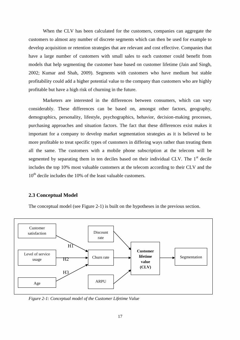
2.3 Conceptual Model
The conceptual model (see Figure 2-1) is built on the hypotheses in the previous section.
H1
H2
H3
Figure 2-1: Conceptual model of the Customer Lifetime Value
Customer
satisfaction
Level of service
usage
Age
Discount
rate
Churn rate
ARPU
Customer
lifetime
value
(CLV)
Segmentation

18
The conceptual model shows how customer satisfaction, loyalty and length of relationship,
level of service usage and customer age affect churn. The margin (ARPU), discount rate
(WACC) and churn rate are then used to calculate the customer lifetime value for the
telecom’s customers, which in turn can then be used to segment the customer database.
2.4 Summary
This chapter describes the situation in the telecommunications industry in Iceland and the
harsh competition in this industry with the arrival of new competitors. The main concept of
the thesis, Customer Lifetime Value, is also covered in this chapter. This concept has been the
focus of many companies in the service industry all over the world and is getting increasing
attention. Companies seek to find out which of their customers have the most value for them
and can then use that information to custom their product selection to the customers’ wants
and needs or to retain those customers which are in most danger of churning.
The CLV model used in this thesis is outlined and its elements explained. Customer
churn is the most important part of this model but at the same time the most difficult to
calculate. There are several determinants of churn which have either a positive or negative
influence on the churn rate and hypotheses are formulated about the determinants. CLV can
then be used to segment the customers for a better overview of the most valuable customers.
Finally, the conceptual model is defined.

19
3. Methodology
3.1 Research Design
The research design and related important issues are discussed in this chapter. This research is
quantitative as hypotheses formulated in the previous chapter will be tested with numerical
data from a customer database owned by the telecom. The sample is described shortly along
with the variables in the analysis. Section 3.4 describes the plan of the analysis, where the
classification methods used for the churn analysis are explained.
3.2 Sample
The objective was to attain a sample that consists of mobile phone customers at the telecom
that is heterogeneous in terms of gender and age. There are two datasets constructed for the
quantitative analysis, one consisted of just over 33000 randomly chosen customers with a
post-paid mobile phone subscription (subscription paid at the end of the month) at the telecom
and the other consisted of around 22000 customers with a pre-paid mobile phone subscription
(where customers have to buy recharges when the previous runs out).
The data used for this research is panel data containing usage histories of mobile
phone subscriptions. The datasets were based on the customer database and call log provided
by the telecom and are monthly aggregated. The sample data set is divided into two parts,
training, and validation or testing sets, before executing the analysis. The models are first
developed on the training set and then the probability models are validated by using the
equation on the testing set. For the post-paid sample, a training sample of 4379 customers was
obtained and a testing sample of 28737 customers. For the pre-paid sample, a training sample
of 5995 customers was obtained and a testing sample of 15906 customers. The samples are
given in more details in Section 4.1.
3.3 Variables
There are several variables in the dataset. The dependent variable in the churn analysis is
churn probability. For post-paid customers, a customer is defined as a churner when he or she
switches telecoms. For pre-paid customers, a customer is defined as a churner when he or she
switches telecoms or has not used the number or made a refill for three consecutive months.
The independent variables are related to the mobile phone customers and can be divided into
20
five categories, customer demographics, billing data, refill history (applies to pre-paid
customers only), calling pattern, and call detail records billed (dcr billed). A list of these
variables can be seen in Table I-1 in Appendix I. The data did not include any previous
targeted marketing efforts or information about competition efforts. Various demographic
variables will be used as control variables in the analysis to see whether they have an effect on
churn or not. These variables include gender, marital status, family size and rate plan among
others. This is discussed further in Section 4.3.
3.4 Plan of Analysis
As discussed in the previous chapter, the individual CLV model consists of three elements.
These are the discount rate, the margin/profit and the churn probabilities. The methods used to
calculate these elements will be discussed in the following sections. The margin (ARPU) is
explained first, then the discount rate. The churn model is discussed last and the two
classification methods used to predict churn. The method for calculating the CLV is discussed
shortly and finally the method for segmenting the mobile phone customer base. The analyses
of data in this research were processed using the Statistical Package for the Social Science
(SPSS 19).
The mobile telecommunications market is divided into business and residential
customers. For this research, the business customers are excluded given that they primarily
use mobile services to earn income and they usually do not decide themselves whether to sign
or extend a subscription contract. Since there is much less available information about pre-
paid customers than post-paid customers, there will be separate analyses for these two groups.
Pre-paid customers are not required to give up their name or any other personal information
so usually the available information is restricted to customer behavior like mobile phone
usage.
3.4.1 Average Revenue per User (ARPU)
As stated in Section 2.2.2, ARPU is calculated each month. For this research, the ARPU is
calculated by summing up the total charges paid by a customer over the three month
observation period and divided by three. This is done for both the post-paid and pre-paid
samples.

21
3.4.2 The Discount Rate (WACC)
The most recent figure for the weighted average cost of capital (WACC) at Telecom X will be
used for the calculation of CLV.
3.4.3 Churn Analysis
Two methods will be used to predict customer churn, logistic regression and classification
trees. These methods have both been widely studied and have good predictive performance
(Neslin et al., 2006; Risselada et al., 2010).
Logistic Regression
Binomial logistic regression was conducted to test the hypotheses formed in chapter 2. This
type of regression has been broadly used and examined in predictive data mining to predict
customer churn in various trades like retail industry, financial services and
telecommunications (Samimi and Aghaie, 2011). This method is chosen since the target
variable, customer churn, is not continuous but discrete or categorical (churn or not churn).
The effect of direct factors (i.e., subscription length, amount of charge, number of calls) on
customer churn can be examined with this method. The customers who are going to churn can
be discovered with the logistic regression and also what the drivers of churn are. The model
was estimated using a fixed set of variables from the dataset as described in section 3.3 above.
The logistic regression is conducted to examine the relationship between the customer
churn which is entered into the model as the dependent variable and the other factors
(including subscription length, amount of charge and number of calls) which were entered as
the independent variables. The basic model for the logistic model can be written as:
(3-1)
where churn is customer churn (a binary class label {0,1}), x is the input data, and the
parameters β0 (intercept) and β1 to βm are estimated with the maximum likelihood (ML)
estimation which is the only method to use for individual level data (Allison, 1999). The
probability of a customer churning increases by the amount that is determined by Equation (3-
1) with a unit increase in the independent variable when the coefficient for the independent
variable is positive. Maximum likelihood estimators have good properties in large samples
and are consistent. This means that the probability that the estimate is close to the true value

22
grows as the sample size gets larger. ML also handles well with data with categorical
dependent variables as in this case (Allison, 1999). The Wald chi-square statistic is used to
test the significance of the individual coefficients that are obtained through the maximum
likelihood estimation (Allison, 1999).
Decision Trees
One machine-learning method that can be used for constructing prediction models from data
are classification trees, also called decision trees. The prediction models are achieved by
partitioning the data space repeatedly and fitting a simple prediction model within each
partition. It is then possible to represent the partitioning graphically as a decision tree (Loh,
2011). Decision trees have attracted great attention from both researchers and practitioners
and have become the most popular data mining tools among managers because of its practical
use (Neslin et al., 2006). The decision tree splits the customer dataset successfully into
mutually exclusive discrete subsets and each customer is assigned to one subset or the other.
(Risslelada et al., 2010). It is an intuitive and easy-to-implement predictive modeling
technique. The trees are a sequence of criteria for classifying customers according to metrics
such as likelihood of churn. The pictorial visualization of a decision tree makes it easy to
operate and communicate (Witten and Frank, 2005). The purpose is to build a tree so that the
values of a categorical dependent variable (churn in this instance) can be predicted based on
the values of the continuous and/or categorical independent variables. The decision tree
algorithms create groups that consist of individuals based on a criterion which is selected for
splitting a group. The groups are called nodes which form a branching node tree. The
dependent variable is at the top of the tree and is the root node. It consists of all cases in the
sample. Each node in the tree can be split into two nodes, called child nodes. The original
node is then the parent node. This partitioning process can be employed repeatedly where
each child node can be split in two. If a node has no child nodes, it is called a terminal node or
a leaf (Harper and Winslett, 2006). An example of a decision tree for churn is shown in Figure
3-1 on the next page. Churn is the root node and the tree splits the customers in the sample in
three groups (nodes 2, 3 and 4). Those customers who are in a family of two or more people
or those who are single males are more likely to be active customers. However single female
customers are more likely to churn.

23
Churn
Family size
1 person 2 people; > 2 people
Gender
Female Male
Figure 3-1: An example of a decision tree for churn
Decision trees can be used for segmentation where people are identified as being
members of a specific group, or for prediction where rules are formed and used to predict
future events like churn, like with the logistic regression. They can also be used to reduce data
and for variable screening where useful subsets of predictor variables are selected from a
larger set of variables. The dependent and independent variables used in creating decision
trees can be nominal, ordinal or scale. There are four methods in SPSS that can be used to
grow the decision trees:
CHAID, which stands for Chi-squared Automatic Interaction Detection where the independent
variable which has the strongest interaction with the dependent variable is chosen.
Exhaustive CHAID, which is a modification of CHAID. It inspects all possible splits for each
predictor or independent variable.
CRT, which stands for Classification and Regression Trees. It splits the data into homogeneous
segments in concern with the dependent variable. The classification tree is generated by using the
Gini index of diversity to choose the best splitting decision for the nodes.
QUEST, which stands for Quick, Unbiased, Efficient Statistical Tree. This method is fast and
evades other method’s bias in support of predictors that have many categories. It can only be
specified if the dependent variable is nominal.
With both the CRT and QUEST methods, a tree can be pruned to decrease the level of
complexity of the tree’s structural design and to avoid overfitting the model. A tree is grown
until the stopping criteria are met. The tree is then trimmed automatically to the smallest
subtree based on the specified maximum difference in risk.
The advantage that decision trees have over other classification methods, including
logistic regression, is that there are no assumptions made regarding the distribution of the
independent variables. They can therefore deal with data that is highly skewed along with
Node 0
Node 1 Node 2
Classification: censoring
Node 3
Classification: churn
Node 4
Classification: censoring

24
categorical independent variables with ordinal or non-ordinal structure. This reduces the time
spent on analysis and the trees are fairly simple to interpret.
3.4.3.1 Model Performance Evaluation
There are several ways to evaluate the performance of a prediction model. Two methods were
used in this analysis, confusion matrix and ROC curve. They are described below.
Confusion Matrix
The classification methods (e.g. logistic regression, decision tree) used produce “raw data”
during testing which are counts of correct and incorrect classifications from each class. This
information can then be presented in a confusion matrix which is a form of contingency table
that illustrates the differences between the true and predicted classes for a set of labeled
examples. A confusion matrix is shown in Table 3-1. It has four possible outcomes, where Tp
and Tn are the number of true positives (a case is positive and classified as positive) and true
negatives (a case is negative and classified as negative) respectively. Fp (also Type I error) are
numbers of false positives, where a case is negative and classified as positive. Fn (also Type II
error) are the number of false negatives, where a case is positive but classified as negative. Cn
and Cp are the row totals and are the number of truly negative and positive examples. Rn and
Rp are the number of predicted negative and positive examples and N is the overall accuracy
(Bradley (1997), Fawcett (2006)).
Table 3-1: Confusion matrix
Predicted class
negative positive
Observed negative Tn Fp Cn
class positive Fn Tp Cp
Rn Rp N
Some significant information can be extracted from the table to illustrate certain
performance criteria.
Positive predictive value (also called hit rate or recall) is the proportion of positive instances
which were classified correctly =
, where Rp = Fp + Tp (3-2)

25
The false positive value (also called false alarm rate) is the proportion of negative instances
which were classified incorrectly as positive =
(3-3)
Negative predictive value is the proportion of negative instances which were classified
correctly =
where Rn = Fn + Tn (3-4)
The false negative value is the proportion of positive instances which were classified
incorrectly as negative =
(3-5)
Sensitivity =
, where Cp = Tp + Fn (3-6)
Specificity =
, where Cn = Tn + Fp (3-7)
N (Overall accuracy) =
or =
(3-8)
In the case of customers at the telecom, those who are in the true positive category are
those who churned and correctly classified as churners. Those in the false positive category
were non-churners classified as churners and those in the false negative category were
churners incorrectly classified as non-churners. Customers in the true negative category were
non-churners correctly classified as non-churners. Sensitivity indicates the model’s capability
to identify positive results (churn). It is the probability of a customer being predicted as
churner, given that the customer has churned. Specificity indicates the model’s capability to
identify negative results (non-churn). This is the probability of a customer being predicted as
non-churner, given that the customer has not churned. A model with high sensitivity has a low
type II error rate while a model with high specificity has a low error I rate. Sensitivity and
specificity are also terms associated with ROC curves which will be discussed next.
The ROC Curve
The Receiver Operating Characteristic (ROC) curve is a helpful technique to visualize the
performance of a classification method (e.g. logistic regression) with the intention to select a
fitting operation point, or decision threshold. A figure is obtained by plotting the performance
of a binary classifier system while the discrimination threshold (cutoff point) is varied. It is a
cross-validated estimate of the classification method’s overall accuracy (probability of a
correct response) (Bradley, 1997). If, for example, the threshold is changed from .5 (the
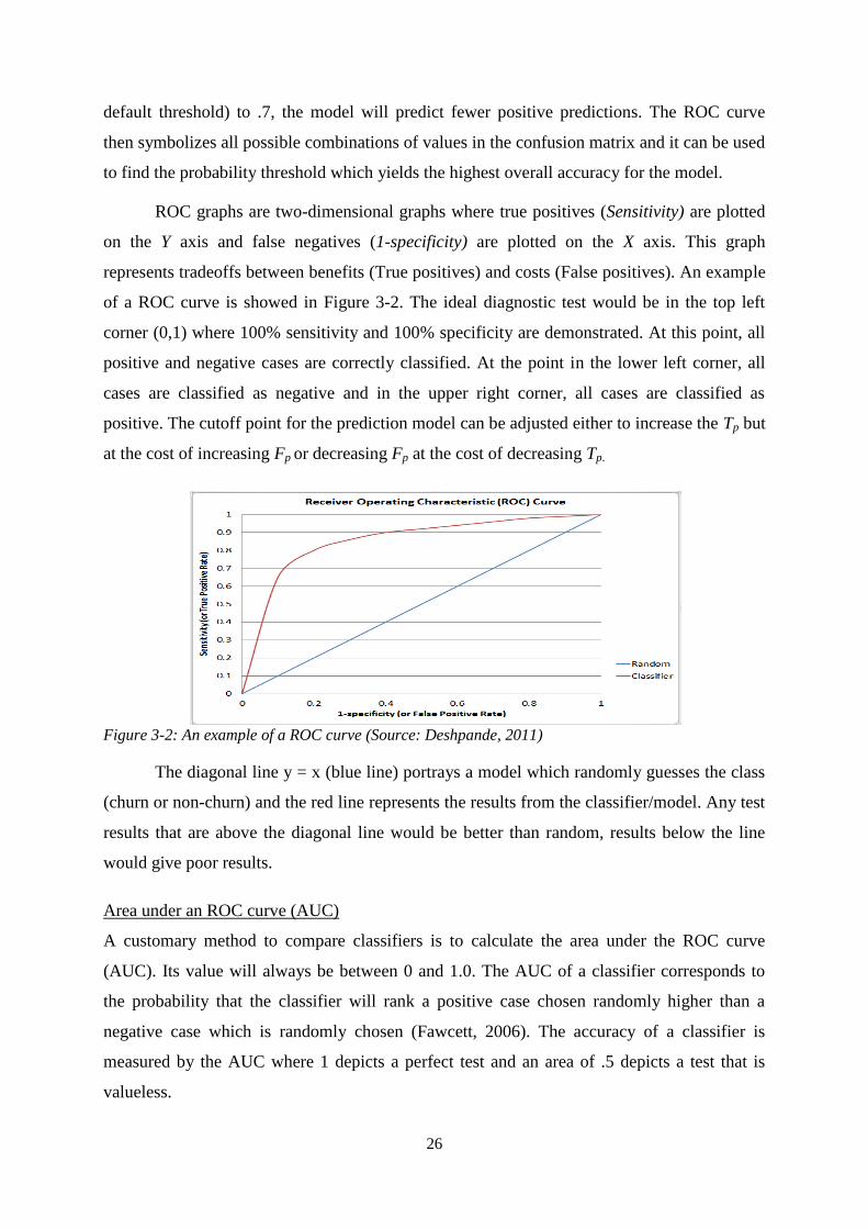
26
default threshold) to .7, the model will predict fewer positive predictions. The ROC curve
then symbolizes all possible combinations of values in the confusion matrix and it can be used
to find the probability threshold which yields the highest overall accuracy for the model.
ROC graphs are two-dimensional graphs where true positives (Sensitivity) are plotted
on the Y axis and false negatives (1-specificity) are plotted on the X axis. This graph
represents tradeoffs between benefits (True positives) and costs (False positives). An example
of a ROC curve is showed in Figure 3-2. The ideal diagnostic test would be in the top left
corner (0,1) where 100% sensitivity and 100% specificity are demonstrated. At this point, all
positive and negative cases are correctly classified. At the point in the lower left corner, all
cases are classified as negative and in the upper right corner, all cases are classified as
positive. The cutoff point for the prediction model can be adjusted either to increase the Tp but
at the cost of increasing Fp or decreasing Fp at the cost of decreasing Tp.
Figure 3-2: An example of a ROC curve (Source: Deshpande, 2011)
The diagonal line y = x (blue line) portrays a model which randomly guesses the class
(churn or non-churn) and the red line represents the results from the classifier/model. Any test
results that are above the diagonal line would be better than random, results below the line
would give poor results.
Area under an ROC curve (AUC)
A customary method to compare classifiers is to calculate the area under the ROC curve
(AUC). Its value will always be between 0 and 1.0. The AUC of a classifier corresponds to
the probability that the classifier will rank a positive case chosen randomly higher than a
negative case which is randomly chosen (Fawcett, 2006). The accuracy of a classifier is
measured by the AUC where 1 depicts a perfect test and an area of .5 depicts a test that is
valueless.

27
3.4.3.2 Model Validation
The logistic regression models and decision models created for post- and pre-paid training
samples will be validated on separate testing samples which are unbalanced to replicate real
world data.
3.4.4 The CLV Calculation
After estimating the average revenue per user, the discount rate and the churn for individual
customers in the data sets, the next step is to use these results and estimate the CLV for each
customer by using model (2-1) discussed in section 2.1.1.
3.4.5 Segmentation
As stated in Section 2.2, the customer database with post-paid and pre-paid subscription at
Telecom X will be segmented based on their individual CLV. There will be ten segments for
each type of subscription, which are of equal size. The 1st decile consists of the least valuable
customers while the most valuable customers are in the 10th
decile. These deciles will be
described to give some insight about what the customers within the deciles have in common.
3.5 Summary
In this chapter, the research design of the thesis was discussed. Next the data sets collected at
the telecom was described shortly, followed by the plan of analysis where the calculation of
ARPU and WACC was explained. Churn analysis was described, where the two methods
used, logistic regression and decision trees were outlined. The models will be evaluated for
prediction accuracy and validated on separated data sets. Then the calculation of CLV was
shown and finally the segmentation was covered.
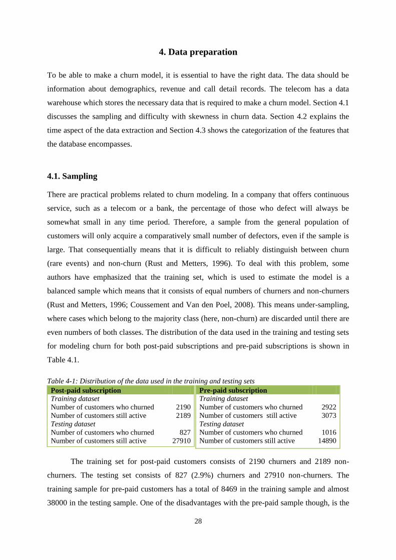
28
4. Data preparation
To be able to make a churn model, it is essential to have the right data. The data should be
information about demographics, revenue and call detail records. The telecom has a data
warehouse which stores the necessary data that is required to make a churn model. Section 4.1
discusses the sampling and difficulty with skewness in churn data. Section 4.2 explains the
time aspect of the data extraction and Section 4.3 shows the categorization of the features that
the database encompasses.
4.1. Sampling
There are practical problems related to churn modeling. In a company that offers continuous
service, such as a telecom or a bank, the percentage of those who defect will always be
somewhat small in any time period. Therefore, a sample from the general population of
customers will only acquire a comparatively small number of defectors, even if the sample is
large. That consequentially means that it is difficult to reliably distinguish between churn
(rare events) and non-churn (Rust and Metters, 1996). To deal with this problem, some
authors have emphasized that the training set, which is used to estimate the model is a
balanced sample which means that it consists of equal numbers of churners and non-churners
(Rust and Metters, 1996; Coussement and Van den Poel, 2008). This means under-sampling,
where cases which belong to the majority class (here, non-churn) are discarded until there are
even numbers of both classes. The distribution of the data used in the training and testing sets
for modeling churn for both post-paid subscriptions and pre-paid subscriptions is shown in
Table 4.1.
Table 4-1: Distribution of the data used in the training and testing sets
Pre-paid subscription
Training dataset
Number of customers who churned 2922
Number of customers still active 3073
Testing dataset
Number of customers who churned 1016
Number of customers still active 14890
The training set for post-paid customers consists of 2190 churners and 2189 non-
churners. The testing set consists of 827 (2.9%) churners and 27910 non-churners. The
training sample for pre-paid customers has a total of 8469 in the training sample and almost
38000 in the testing sample. One of the disadvantages with the pre-paid sample though, is the
Post-paid subscription
Training dataset
Number of customers who churned 2190
Number of customers still active 2189
Testing dataset
Number of customers who churned 827
Number of customers still active 27910

29
proportion of missing data. Since customers with a pre-paid subscription do not need to
submit personal demographic information about themselves, demographic variables are those
with the most missing data or up to 40%. To find out if there is a significant difference
between those customers with demographic information and for those without it, independent-
samples t-tests were done with all the independent continuous variables. The results were that
the means for the independent variables for the two groups were not the same, except for 1
variable, “Average voice outin volume ratio”. Since there is a difference between these two
groups, it is likely that it will be necessary to make a separate logistic regression model for the
two groups as it is always difficult to fill in missing values, especially for those variables with
only two groups like “Gender”. The decision was therefore taken to exclude those customers
with no demographic information in both the training and testing sets. The final training set
consisted of a total of 5995 customers, 2922 who churned and 3073 which did not. The testing
dataset consisted of 1016 churners (6.4%) and 14890 who were still active. The proportion of
those who churned with respect to those who did not is higher in the two data sets combined
for pre-paid customers, with 17.98% churners. In the two combined post-paid datasets, there
are 9.11% churners. One possible reason for this difference could be that it is easier for pre-
paid customers to terminate their subscription at the telecom and they could therefore be more
prone to follow a better offer at another telecom. Average age is lower for the pre-paid data
sets (37 years in the training set and 40 years in the testing set) than for the post-paid data sets
(49 years in the training set and 52 years in the testing set). This could be a signal of younger
people being less loyal than older people.
4.2. The time aspect
To select the data needed for predicting churn, a time window is used that consists of an
observation period where features for each customers is extracted and a performance period
where customers are labeled as churn or non-churn (see Figure 4-1 on the next page). The
length of the time frame used for analysis can vary and depends on the industry under
inspection. The observation period was set for three months where monthly aggregated
transaction activity and other information were gathered for each customer. Kumar et al.
(2007) found that the optimal performance period was three months for a telecom company
but for this research a performance period of five months was used where the customers were
followed. The customers are then labeled either as churn or censoring (non-churn) since the
timeline is censored, what happens after the performance period is unknown. Customer A in
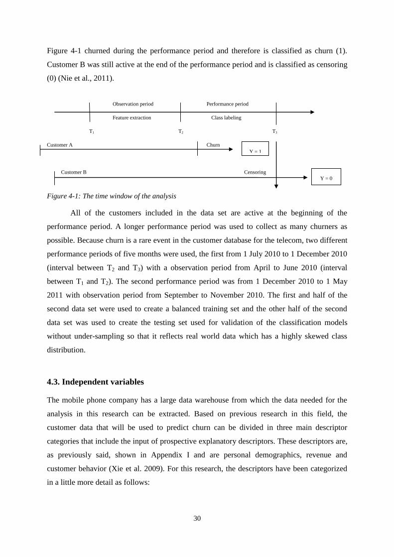
30
Figure 4-1 churned during the performance period and therefore is classified as churn (1).
Customer B was still active at the end of the performance period and is classified as censoring
(0) (Nie et al., 2011).
Observation period Performance period
Feature extraction Class labeling
T1 T2 T3
Customer A Churn
Customer B Censoring
Figure 4-1: The time window of the analysis
All of the customers included in the data set are active at the beginning of the
performance period. A longer performance period was used to collect as many churners as
possible. Because churn is a rare event in the customer database for the telecom, two different
performance periods of five months were used, the first from 1 July 2010 to 1 December 2010
(interval between T2 and T3) with a observation period from April to June 2010 (interval
between T1 and T2). The second performance period was from 1 December 2010 to 1 May
2011 with observation period from September to November 2010. The first and half of the
second data set were used to create a balanced training set and the other half of the second
data set was used to create the testing set used for validation of the classification models
without under-sampling so that it reflects real world data which has a highly skewed class
distribution.
4.3. Independent variables
The mobile phone company has a large data warehouse from which the data needed for the
analysis in this research can be extracted. Based on previous research in this field, the
customer data that will be used to predict churn can be divided in three main descriptor
categories that include the input of prospective explanatory descriptors. These descriptors are,
as previously said, shown in Appendix I and are personal demographics, revenue and
customer behavior (Xie et al. 2009). For this research, the descriptors have been categorized
in a little more detail as follows:
Y = 1
Y = 0

31
1. Demographics are personal data of a given costumer, such as age, gender, marital status, place
of residence, family size, rate plan, whether or not the customer is the registered payer and
tenure which is the number of days a customer was or is active and finally customer status
which says whether or not he/she churned or not. The variable “Rate plan” had up to 20
different categories where some categories had many cases and other categories had very few
cases. For this reason, it was impossible to use this variable and it was removed from the
analysis.
2. Billing data shows the number of billed services, number of billed products, billed amount due
to mobile phone usage, discount amount a customer receives, total billed amount and ratio of
both mobile usage and discount versus total billed amount. These variables apply only to post-
paid customers.
3. Refill history applies only to customers with pre-paid subscriptions. These descriptors are
refill frequency and amount and total refill frequency and amount.
4. Calling pattern are descriptors created for both post-paid and pre-paid customers. They are
related to inside and outside network and abroad call volume and frequency, total originating
and terminating call volume and frequency, total sent and received text messages, ratio of
inside/outside network and abroad calls versus total originating call volume/frequency, ratio of
originating calls versus terminating call volume and ratio of text messages sent versus text
messages received.
5. CDR (call detail records) billed are descriptors of charged amount due to inside/outside
network and abroad calls, ratio of inside/outside network and abroad calls versus total charged
amount, charged amount due to text messages sent inside/outside network and abroad, ratio of
inside/outside network and abroad text messages sent versus total charged amount and then
total charged amount. These are also created for both types of subscriptions.
Besides the above mentioned descriptors, there are also derivatives such as the maximum
value over the three months and average value over the three months. These features are also
all listed in Appendix I. The demographic features are extracted at the beginning of the
observation period but the features in the other categories are extracted for each of the three
months of the observation period.
4.5 Summary
In this chapter, data preparation has been detailed. There was a large set of information to go
through for both pre-paid and post-paid customers and therefore necessary to examine them
well before the main analysis. A sizeable proportion of missing values existed in the pre-paid
datasets and as there was a difference between customers who submitted demographic
information and those who did not, cases with missing values were excluded.

32
The time aspect of the research is then outlined in the next section. Two time windows
of eight months each were used in the research, where the observation period was three
months and the performance period was five months. Finally, further details are given about
the independent variables which are numerous in the data sets related to demographics, billing
data, refill history, calling pattern and call detail records.

33
5. Results
The results from the analysis are presented in this chapter. Firstly, the sample with the post-
paid customers will be described in Section 5.1 and the results shown, both for the training
and testing samples. Then results for the pre-paid customers are presented in Section 5.2, both
for the training and testing samples. The outcomes of the hypotheses presented in chapter 2
are discussed in Section 5.3. Finally, the results from the CLV calculations and the
segmentation are presented and discussed in Section 5.3.
5.1 Post-paid customers
5.1.1 Sample description
In this chapter the sample of post-paid customers at the telecom is analyzed. These are
customers who receive their bill at the end of each month. The sample used to training the
churn model consisted of 2190 churners and 2189 non-churners or total of 4379 post-paid
customers.
Since non-churners are still active customers with the telecom, it is impossible to
calculate mean values for the independent variables such as tenure as this will continue to an
unknown date in the future. Therefore the mean values are calculated for the time period that
is used to extract the data. The mean for the customers’ age was 49.19 years (with a SD =
14.828). The youngest customer is 18 years of age and the oldest customer is 98 years of age.
There were more males than females in this sample or 2488 (56.8%) and 1891 respectively.
Table 5-1 shows the marital status of the customers. Most of them are married/in a registered
partnership (53.2%). 28.9% are unmarried, 11.8% are either divorced or separated and 5.0%
widowed. Customers with an unknown status were 0.6% of the sample.
Table 5-1: Marital status of customers in the post-paid training sample
Marital status Frequency Percent Cumulative %
Married/registered partnership 2328 53.2 53.2
Unmarried 1265 28.9 82.1
Divorced 441 10.1 92.2
Widowed 218 5.0 97.2
Separated
Other
Marital status unknown
73
26
28
1.7
0.6
0.6
98.9
99.5
100.0
Total 4379 100.0
Two categories “Married (not living together)” and “Icelander living abroad” were
combined into 1 category “Other” since there were so few in each category. This category

34
consists of 26 customers or 0.6%. Regarding the customers’ family size, which is shown in
Table 5-2, most customers in the sample were single individuals or 3244 (74.1%). 922 were in
a family consisting of 2 people, 169 in a family of 3 people, 35 were in a family of 4 people
and 9 were in a family of 5 people or more. Because there is a large difference in the
frequencies in the first two categories and the last three, these last three categories where
combined into one. The third category includes 213 customers or 4.9% of the sample.
Table 5-2: Family size of customers in the post-paid training sample
Family size Frequency Percent Cumulative %
1 person 3244 74.1 74.1
2 people 922 21.1 95.1
3 people or more 213 4.9 100.0
Total 4379 100.0
The customers were fairly dispersed over the country, considering that 2/3 of the
Icelandic population lives within the greater capital area of Reykjavik. Table 5-3 shows the
distribution of the sample over the country. The majority of the customers live within the
greater capital area, or 2516 (57.4%) followed by 668 customers who live in the Southern part
Table 5-3: Residence of customers in the post-paid training sample
Land area Frequency Percent Cumulative %
Capital area 2516 57.5 57.5
Western Iceland 365 8.3 65.8
Northern Iceland
Eastern Iceland
Southern Iceland
Unknown
592
177
668
61
13.5
4.0
15.3
1.4
79.3
83.4
98.6
100.0
Total 4379 100.0
of Iceland. 61 customers have an unknown location. The mean for tenure, which refers to the
amount of days that an individual was or has been a customer, was 2177 days (SD = 1752.5).
The maximum number of days was 5917 (approximately 16 years) and the minimum number
of days was 31. The average number of various additional services (besides the basic post-
paid service itself) offered by the telecom that customers bought, was 3 (SD = 2.54). The
maximum number of services bought was 59 and some customers bought no additional
services. For the number of various products bought, the average was 29.8 (SD = 21.4), where
the maximum number of products bought was 149.7 and some customers bought none.
Examples of services and products are any additional services or products customers can add
to their subscription like mobile internet, calling friends for free, internet at home, land line
and television.

35
Table 5-4 shows the results from a chi-square test for independence. This test was
done to explore the relationship between customers’ status (churn or non-churn) and other
categorical variables. This table shows how many females and males churned or 991 (52.4%
of the females) and 1199 (48.2% of the males) respectively. For a 2x2 table like this, there can
be overestimation of the chi-square value but the Yates’ Correction for Continuity
compensates for that. The value is 7.467, with 1 degree of freedom (df) with an associated
significance level of .006 which is smaller than the alpha value of .05 (see Table II-1 in
Appendix II). The conclusion is made that the proportion of males who churn is significantly
different from the proportion of females who churn. However the value of Phi is -.042 (p =
.006) which indicates that the relationship between the two variables in the table is weak (see
Table II-2 in Appendix II).
Table 5-4: Crosstable of Status*Gender in the post-paid training sample Gender
Total Female Male
Status Non-churn Count 990 1289 2189
% within gender 47.6% 51.8% 50.0%
Churn Count 991 1199 2190
% within gender 52.4% 48.2% 50.0%
Total Count 1891 2488 4379
% within gender 100.0% 100.0% 100.0%
The same test was also done for family size, land area, whether or not the customer is
the payer, marital status and total charge groups. Since the other demographic variables,
except “Is payer”, have 3 or more categories, Cramer’s V is the appropriate statistic instead of
phi. For “Family size”, the Pearson Chi-square from Chi-Square tests is 14.454 with a p =
.001 (df = 2). This means that there is a significant difference in status (churn or non-churn)
and number of people in the family. The Cramer’s V is 0.057 (p = .001) which indicates a
weak relationship between the two variables. The Chi-square for “Land area” is 64.788 and p
= .001 (df = 5). The Cramer’s V is 0.122 (p = .001). So like with the former variables, there is
a difference in status and residence and the relationship is somewhat stronger. For “Marital
status”, the Pearson Chi-square is 90.961 with p = .001 (df = 6). The Cramer’s V is 0.144 (p =
.001). For “Total charge groups”, the Pearson Chi-square is 265.911 and p = .001 (df = 1).
The Cramer’s is 0.246 (p = .001). The variable “Is payer” was the only demographic variable
where the results were not significant. As this variable only has two categories, yes or no, the
results are a 2x2 table. Therefore the value for Continuity Correction from the Chi-Square
tests is used. This value is 1.531 with p = .248 (df = 1). The phi is 0.019 (p = .216). This

36
means that the proportion of those who churn is not significantly different from the proportion
of those who are still active.
To see if there was a significant difference in the mean of different continuous
variables for those who churned and those who did not, an independent samples t-test was
done (see Table II-3 in Appendix II). Out of the 42 variables regarding customer age, tenure
and averages, 34 of them had a significance level for the Levene’s test lower than .05
indicating that the variance of scores for the two groups (churners and non-churners) is not the
same. The variables where there was no significant difference in the variance were “Average
amount gsm”, “Average ratio gsm”, “Average abroad total charge ratio”, “Average text
message innet total charge ratio” and “Average text message abroad total charge ratio”. For
the t-test for equality of means, which says whether there is a significant difference between
those who churned and those who did not, eight variables had a significance value higher than
.05. For all the other variables, there is a significant difference in the mean values between the
two dependent groups (churn and non-churn). The eight insignificant variables were “Average
ratio gsm”, “Average abroad volume”, “Average abroad volume ratio”, “Average abroad
frequency ratio”, “Average voice outin volume ratio”, “Average abroad total charge ratio”,
“Average text message abroad charge” and “Average text message abroad total charge ratio”.
Of the 33 variables with maximum values, three of them had a significance level for the
Levene’s test higher than .05 indicating the variance of scores for churners and non-churners
were the same. These variables were “Maximum abroad total charge ratio”, Maximum text
messages innet total charge ratio” and “Maximum text messages abroad total charge ratio”.
Eight variables had a p > .05 for the t-test for equality of means so there was not a significant
difference in the mean values between the two dependent groups. These variables were
“Maximum voice outin volume ratio”, Maximum abroad volume”, Maximum abroad volume
ratio”, Maximum abroad frequency ratio”, “Maximum innet total charge ratio”, “Maximum
abroad total charge ratio”, “Maximum text messages abroad charge” and “Maximum text
messages abroad total charge ratio”.
Finally, to find out the effect size statistics, eta squared is calculated. This implies the
magnitude of the differences between the two status groups. The equation for eta squared is
Eta squared
(5-1)

37
where,
t the t-value from the t-test for equality of means
N number of individuals in each group
When the outcome of this formula is multiplied with 100, it can be expressed as a
percentage. The values of eta range from an extremely low value of 5.78*10-7
to 0.08294 so
the effect size is extremely small to medium. For the variable with the highest eta value,
“Average outnet frequency ratio”, 8.294% of the variance in that variable is explained by
customer status, for the other variables the percentage is less than that.
5.1.2 Multicollinearity
The presence of multicollinearity in the data can be a problem as it can affect the parameters
of the regression model. Correlation between any two independent variables should not be too
high (Field, 2009). To check whether multicollinearity is an issue in the data, one can look at
the tolerance and VIF (Variance Inflation Factor) statistics which are obtained from linear
regression using the same dependent and independent variables as in the logistic regression. A
tolerance value < 0.1 and a VIF value > 10 imply a serious collinearity problem (Field, 2009;
Menard, 2001). This procedure was followed by using all 82 independent variables, both
demographics and usage variables. 63 out of 66 variables, which were related to mobile phone
usage, had a tolerance value < 0.1 revealing that there is an issue with multicollinearity in the
data. However all of the demographics had a tolerance > 0.1. It is difficult to determine the
best manner of dealing with multicollinearity as it is impossible to know which variable
should be left out. One option would be to run a factor analysis on those variables involved in
the multicollinearity and use the factor scores as a predictor. Another option would be to
acknowledge the unreliability of the model (Field, 2009; Tabachnick and Fidell, 2001). The
decision was taken to run a principal component analysis on all 66 usage variables.
5.1.3 Principal component analysis
To see if the 63 variables which were involved in the multicollinearity form coherent subsets,
a Principal Component Analysis (PCA) with Varimax rotation was performed, but the
decision was made to use all 66 variables related to usage in the PCA. Those variables that
correlate with one another are combined into subsets or components which are independent of
other subsets. The PCA method is the only method where multicollinearity is not a problem

38
which is the reason why it was chosen for this analysis (Field, 2009; Tabachnick and Fidell,
2001).
As mentioned before, 66 variables were used in the PCA. These items were related to
usage and charges, both inside and outside the telecom’s network and abroad (see Table II-4
in Appendix II for the list of variables used). After the initial run, the Kaiser-Meyer-Olkin
measure confirmed the sampling adequacy for the analysis (KMO = .811) and the Bartlett’s
test of sphericity χ2 = 691523.602, with df = 2145 and p = .001. This implies that correlations
between the variables are large enough to conduct PCA (Field, 2009). Two variables,
“Average voice outin volume ratio” and “Maximum voice outin volume ratio”, had individual
KMO values < .5 (from the Anti-image Matrices) so the latter variable was removed. In the
second run with 65 variables, all variables had KMO values > .5 and their communalities
were from .572 and over which implies that they are all applicable for the analysis. According
to the Kaiser’s criterion of eigenvalues over 1, 12 components would be a suitable solution
and together they explained 87.766% of the variance in the data. The scree plot (shown in
Figure II-1 in Appendix II) showed a point of inflexion 2, 4, 5, 7, 11, 12, 16 and 22
components meaning that a solution with 1, 3, 4, 6, 10, 11, 15 or 21 components would be
appropriate. After extraction, the components are usually rotated in order to maximize high
correlations and minimize the low ones. The most frequently used method of rotation is
Varimax which is an orthogonal rotation. This method simplifies components by maximizing
the variance of factor loadings by making high loadings higher and low loadings lower for
each component (Agresti and Finlay, 1997). The analysis was run again, extracting 12
components, based on Kaiser’s criterion. To make the rotated component matrix easier to
interpret, coefficient values below .3 were suppressed. When the rotated component matrix
was checked, some items had only low loadings in two or more components (difference in
loadings over components less than .2) which made it difficult to decide in which component
to place these items. The analysis was then rerun, taking one variable out at a time until all
items loaded highly on only one component. By taking out variables, three components
consisted of only low loadings so the components were reduced to nine. The final solution
consisted of 53 items after omitting 13 items altogether which loaded on nine components.
5.1.3.1 Internal consistency reliability analysis
To assess reliability of a multi-item scale, the method that is mostly used is an evaluation of
the scale’s internal consistency reliability. The Cronbach’s alpha is an index which is a

39
method widely used and it should be > .7 to be acceptable (Polit, 2010). Table 5-5 shows the
results of the consistency reliability analysis for eight of the nine components. The first
column shows the number of the component, the second column shows the number of items
in each component and the third column shows the value for Cronbach’s alpha.
Table 5-5: Cronbach’s alpha for the components for the post-paid training sample Component N of items Cronbach’s
alpha
1 21 .911
2 6 .979
3 6 .963
4 5 .000
5 4 .653
6 4 .641
7 4 .571
8 2 .827
The Cronbach’s alpha for component 4 was .000 but would increase to .916 if the item
“Average abroad volume” was deleted. For component 5 it was .635 but increased to .714
when “Maximum text message outnet total charge ratio” was deleted. Component 6 had an
alpha = .641 but increased to .721 by deleting “Maximum text message innet total charge
ratio”. For component 7, the alpha was .571 and would not increase by deleting an item. It
was not possible to calculate the Cronbach’s alpha for the ninth component as it only consists
of one item. Cronbach’s alphas are then acceptable for all components except the seventh.
The alpha coefficients are essential indicators of the quality of the instrument so high
reliability is crucial to success in hypothesis testing (Polit, 2010). Therefore eight components
were used in the proceeding analysis as the one component was excluded due to low alpha.
5.1.3.2 Results from the PCA
After deleting the seven variables mentioned in the previous section, the PCA was rerun using
46 variables. The variables omitted from the analysis are shown in Table II-5 in Appendix II.
As mentioned above, Kaiser’s criterion of eigenvalues over 1 is often used to determine the
number of factors in PCA along with the scree plot. In this case, as shown in Table II-6 in
Appendix II, nine components had eigenvalues > 1. As previously stated, a solution with nine
or more components did not make sense as they would only include low loadings and the
Cronbach’s alpha was too low for one of the components. Therefore the decision was made to
continue with eight components and they explained 89.154% of the total variance in the data
(see Table II-6 in Appendix II). The KMO measure for this final analysis was .830 and the
Bartlett’s test of sphericity χ2 = 475859.216 (df = 1035, p = .001). Communalities and the

40
individual KMOs (item communalities) were all > .5. These values signify the amount of
variance in the item that is explained by the extracted components (Pett et al, 2003). As there
are no χ2
goodness-of-fit tests on hand for PCA, a comparable function can be executed by
examining the residual correlation matrix. This matrix is created by subtracting the
reproduced correlation matrix which is produced by the components from the actual
correlation matrix. The table “Reproduced Correlations” produced by SPSS showed residuals
that are the difference between actual and reproduced correlations as explained earlier. The
residuals give an indication about the goodness of fit for the analysis. 11% (156) of the
residuals had absolute values > .05 which is well below 50% of all the residuals. This
conclusion indicates that the extracted component solution represents a good fit for the data
(Pett et al, 2003).
The resulting components are shown in Table II-7 in Appendix II, which is the rotated
component matrix generated using the Varimax rotation. In general, the emerged component
structure was quite clear and easy to interpret. The first component is largest and accounted
for 36.296% of the variance. It had 21 items which can be seen in the table (only loadings
above .3 are shown to simplify it). It represents both average and maximum values (over the
five month observation period) of usage and charges both within and outside of the telecom’s
network and average and maximum total originating and terminating phone calls. The second
component had a variance of 17.059% and had six items. It represents average and maximum
ratios related to usage and charge outside the telecom’s network. The third component had a
variance of 9.138% and consisted of six variables with average and maximum ratios related to
usage and charge inside the telecom’s network. The fourth component had a variance of
7.821% and consisted of four variables related to usage abroad ratios. The fifth component
had a variance of 6.789% and consisted of three variables with charges for sending text
messages outside the telecom’s network. The sixth component had a variance of 3.775% and
consists of three variables with charges for sending text messages inside the telecom’s
network. The seventh component had a variance of 3.298% and consisted of two variables of
charges for sending text messages abroad. The eighth component had a variance of 2.684%
and consisted of one item which is the ratio between originating and terminating call volume.
The following description of the eight components is based on the items in each of them:
Component 1: Usage/charges inside and outside the telecom’s network
Component 2: Usage/charge ratios outside the telecom’s network
Component 3: Usage/charge ratios inside the telecom’s network
Component 4: Usage ratios abroad
Component 5: Text message charge ratios outside the telecom’s network
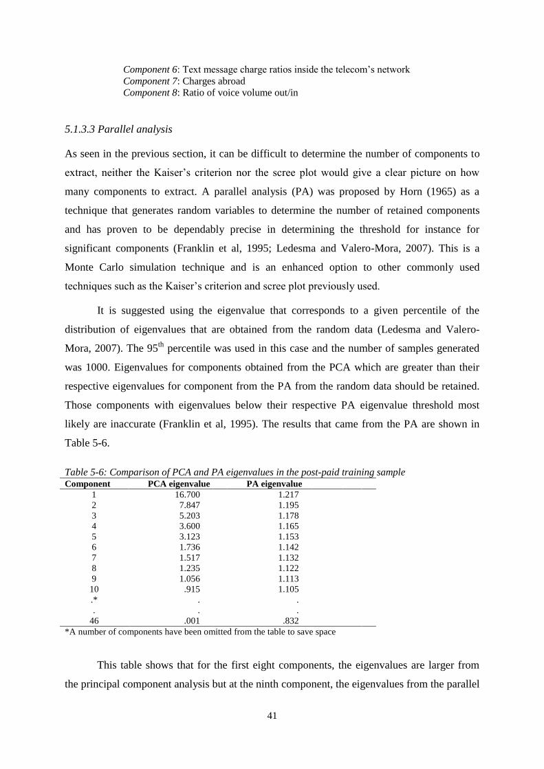
41
Component 6: Text message charge ratios inside the telecom’s network
Component 7: Charges abroad
Component 8: Ratio of voice volume out/in
5.1.3.3 Parallel analysis
As seen in the previous section, it can be difficult to determine the number of components to
extract, neither the Kaiser’s criterion nor the scree plot would give a clear picture on how
many components to extract. A parallel analysis (PA) was proposed by Horn (1965) as a
technique that generates random variables to determine the number of retained components
and has proven to be dependably precise in determining the threshold for instance for
significant components (Franklin et al, 1995; Ledesma and Valero-Mora, 2007). This is a
Monte Carlo simulation technique and is an enhanced option to other commonly used
techniques such as the Kaiser’s criterion and scree plot previously used.
It is suggested using the eigenvalue that corresponds to a given percentile of the
distribution of eigenvalues that are obtained from the random data (Ledesma and Valero-
Mora, 2007). The 95th
percentile was used in this case and the number of samples generated
was 1000. Eigenvalues for components obtained from the PCA which are greater than their
respective eigenvalues for component from the PA from the random data should be retained.
Those components with eigenvalues below their respective PA eigenvalue threshold most
likely are inaccurate (Franklin et al, 1995). The results that came from the PA are shown in
Table 5-6.
Table 5-6: Comparison of PCA and PA eigenvalues in the post-paid training sample Component PCA eigenvalue PA eigenvalue
1 16.700 1.217
2 7.847 1.195
3 5.203 1.178
4 3.600 1.165
5 3.123 1.153
6 1.736 1.142
7 1.517 1.132
8 1.235 1.122
9 1.056 1.113
10 .915 1.105
.*
.
46
.
.
.001
.
.
.832
*A number of components have been omitted from the table to save space
This table shows that for the first eight components, the eigenvalues are larger from
the principal component analysis but at the ninth component, the eigenvalues from the parallel

42
analysis become larger. These results suggest that an eight component solution would be
appropriate, supporting the previous results obtained from the principal component analysis.
5.1.4 Logistic regression
After dealing with the multicollinearity in the dataset by running a PCA, the next step is the
logistic regression, as there was not an issue with multicollinearity among the components. A
logistic model is fitted to the data to test the research hypotheses previously stated concerning
the relationship between the likelihood that a customer will churn and various features related
to his or her demographics and telephone usage. These variables are related to demographic
information along with the eight components from the PCA. Multicollinearity was also
checked for among the 20 variables omitted from the PCA analysis (see Table II-5 in
Appendix II) and 15 of them did not have this problem. The variables “Maximum text
messages in”, “Maximum text messages out”, “Maximum abroad volume”, “Maximum
abroad frequency” and “Maximum text messages abroad charge” were excluded based on
high VIF/low tolerance values. In all, 38 variables were used in the following analysis.
First, all 38 variables and components were entered into the logistic regression (see
Table II-8 in Appendix II of the variables used). Since the decision to include the independent
variables was based on prior knowledge and research, the method used was Enter, which
forces all variables into the model in one block. After the first run, several of the variables
were insignificant with a p > .05 (see Table II-9 in Appendix II). One of these insignificant
variables was removed at a time, based on the highest p-value and the regression run again.
The final model consisted of 13 statistically significant variables, related to demographics,
usage/charges and components. The variables included in the final model are shown in Table
5-7. The groups in the categorical variables that are significant are marked with a *.
Table 5-7: Results from the logistic regression for the post-paid training sample
B
S.E.
Exp(B)
95% C.I. for Exp(B)
Lower Upper
Constant
Customer age
Family size: 1 person
Family size: 2 people*
Family size: 3 people or more
1.179
-0.028
-1.95
-0.330
0.162
0.003
0.086
0.175
3.253
0.973
0.823
0.719
0.968
0.695
0.510
0.978
0.974
1.013
Land area: Capital area
Land area: Western Iceland
Land area: Northern Iceland
-0.064
-0.086
0.124
0.101
0.938
0.919
0.735
0.754
1.196
1.121
Land area: Eastern Iceland* -1.112 0.195 0.329 0.224 0.482
Land area: Southern Iceland -0.018 0.096 1.019 0.844 1.230
Land area: Unknown -0.009
0.303 0.991 0.547 1.797

43
Tenure 3 years
Average number of services
Average number of products/5
Average abroad total charge ratio
Maximum text messages outnet total charge ratio
Total charge groups: Heavy users
C1: Usage/charges in-/outside network
C2: Usage/charge ratios outside network
C3: Usage/charge ratios inside network
C4: Usage ratios abroad
-0.073
-0.031
0.042
0.705
1.310
0.226
0.205
0.526
0.205
-0.095
0.023
0.026
0.016
0.334
0.421
0.094
0.048
0.038
0.038
0.043
0.930
0.945
1.063
2.024
3.707
1.253
1.228
1.691
1.227
0.909
0.888
0.899
1.030
1.052
1.623
1.043
1.117
1.571
1.139
0.835
0.973
0.994
1.097
3.894
8.468
1.506
1.350
1.821
1.322
0.990
Note: R2 = .129 (McFadden’s ρ
2), .163 (Cox & Snell), .218 (Nagelkerke). Model χ
2 = 718.449, p < .001.
The groups marked with * are statistically significant at the .05 level.
Table 5-7 shows the regression coefficients under the heading B, the standard errors,
the odds ratios under the heading Exp(B) and the 95% confidence interval around the odds
ratio. There are a number of ways to measure the strength of association for a model and they
are an analog to R2 in multiple linear regression. The value for Cox and Snell R
2 was .163.
This measure is based on log-likelihoods and also takes into account sample size. The
Nagelkerke R2 was higher, or .218. McFadden’s ρ
2, which is intended to mimic an R
2, is
another way to test the strength of association. The equation is:
ρ2 =
(5-2)
where,
LL(B) the -2 Log likelihood value for the final model
LL(0) the -2 Log likelihood value for the baseline model including only the constant
The value for the final logistic model was .129 but this measure tends to be much
lower than R2
for multiple regression (Tabachnick and Fidell, 2001). The model had a baseline
model with a -2Log likelihood value of 6070.583 which signifies the fit of the most basic
model, including only the constant, to the data. After entering all nine variables into the model
the -2Log likelihood value became lower, or 5321.468 which indicates that the model
including the independent variables has a better predicting power than when it includes only
the constant. The model was significant with a chi-square = 781.449 (df = 18, p = .001). The
Hosmer and Lemeshow Test is a goodness of fit test which aids to determine whether the
model is correctly specified, that is, how well the model fits the data. If the p-value is below
.05, the model is rejected, indicating a poor model fit. For the final model, the p = .004 which
is significantly lower than the .05 level (chi-square = 22.778, df = 8). The Hosmer and
Lemeshow test has however received some criticism when applied to large datasets as it tends
to give a low p-value although the model fits the data well.

44
5.1.4.1 Results of the logistic regression
The results from the logistic regression imply that in this sample of customers, as the age of a
customer increases by one year, he or she is 0.97 less times likely to churn, with other factors
controlled. This means that the older the customers get, the likelihood that they churn
decreases. For the variable “Family size”, group 2 was significant. This implies that
customers in a family of 2 people are 0.82 times less likely to churn than customers living
alone. For “Land area”, only group 4 was significant, so those customers who live in the
Eastern part of Iceland are 0.33 times less likely to churn to those who live in the base area,
which is the capital area. “Tenure” has virtually no effect as the “B” value is 0.000. Since this
variable shows for how many days a customer has been active, a 1 day increase is a very little
change. To see if it made a difference, a new variable was computed by dividing “Tenure”
with 365 to get a variable based on 1 year. When this variable was entered into the model, the
B value = -0.024 (SE = .008) and customers are 0.977 times less likely to churn as the
variable increases by 1 year. By making a “Tenure” variable based on 3 years, the “B” value =
-0.073 and customers are 0.930 times less likely to churn as the variable increases by three
years. This shows that as a customer stays longer, the less likely he or she is in churning. The
decision was taken to have “Tenure” based on three years in the final model and is shown in
Table 5-7.
The next variable in the table is “Average number of services” over the three months
observation period. As a customer buys one more service, the likelihood that he or she will
churn is 0.945 times less likely. The next variable is “Average number of products”. For every
unit increase in the average number of products that a customer buys, the likelihood of churn
is 1.012 times more likely. However, since the “B” value for this variable is rather small
(0.012) it only adds a negligible amount to the prediction of churn and has the least effect on
churn of all the significant variables. Making this variable based on five products, the “B”
value increased to 0.061 so the effect of this variable is somewhat higher. As the variable
increases by five products, a customer is 1.063 times likelier to churn. Out of the 15 variables
omitted from the PCA analysis, two of them ended in the final model. The former was
“Average abroad total charge ratio”. As this variable increases by 1 unit, customers are 2.02
times more likely to churn. In essence, this means that the more customers pay for usage
abroad, the more likely they are to churn. The latter variable, “Maximum text messages outnet
total charge ratio” has the largest effect on churn with a “B” value of 1.310. There is a 3.7
higher likelihood that a customer churns when the value for this variable increases by 1 unit.

45
Thus, the higher the maximum amount of total charge for sending text messages outside the
telecom’s network, the more likely the customer is to churn. For “Total charge groups”, where
the customers have been divided into two groups, light and heavy users, the odds of a
customer churning are 1.25 times higher for heavy users than light users. Those that use the
mobile phone and other products and services at the telecom more and therefore get larger
billed amounts, are most likely more unsatisfied with paying so much and therefore likelier to
churn. The first of the components that was significant was Component 1: Usage/charges
inside/outside the telecom’s network. When this component increases by 1 unit, customers are
1.2 times more likely to churn. As Component 2: Usage/charge ratios outside the network
increases by 1 unit, customers are 1.7 times likelier to churn. As Component 3: Usage/charge
ratios inside the network increases by 1 unit, customers are 1.23 times more likely to churn.
And finally, for Component 4: Usage ratios abroad, when it increases by 1 unit, a customer is
0.91 times less likely to churn.
The proportion of cases that were correctly classified is shown in Table 5-8 on the
next page. This table documents the validity of predicted probabilities. The rows show the
observed or actual values of the dependent and the columns show the predicted values.
According to this table, with a cutoff point at .5, of the 2189 customers who did not churn, the
model correctly classified 1376 of them as non-churn. The model did better on predicting
those who would churn or 1564 of 2190. This was also supported by the magnitude of
sensitivity (71.4%) in contrast to that of specificity (62.9%). The former measures the
proportion of events (churn) that were correctly classified while the latter measures the
proportion of correctly classified nonevents (non-churn). The false positive rate, which
measures the proportion of cases misclassified as events or churn over all of those classified
as events, is 37.1%. The false negative rate, 28.6%, measures the proportion of cases
misclassified as nonevents or non-churn over all of those classified as nonevents (Peng et al,
2002). The calculations based on equations (3-2) to (3-8) are shown beneath Table 5-8. The
negative predictive value was 68.7% and the positive predictive value was 65.8%.
The overall rate of successful classification was 67.1% which is a moderate
improvement on the 50% correct classification with the model that includes only the constant.
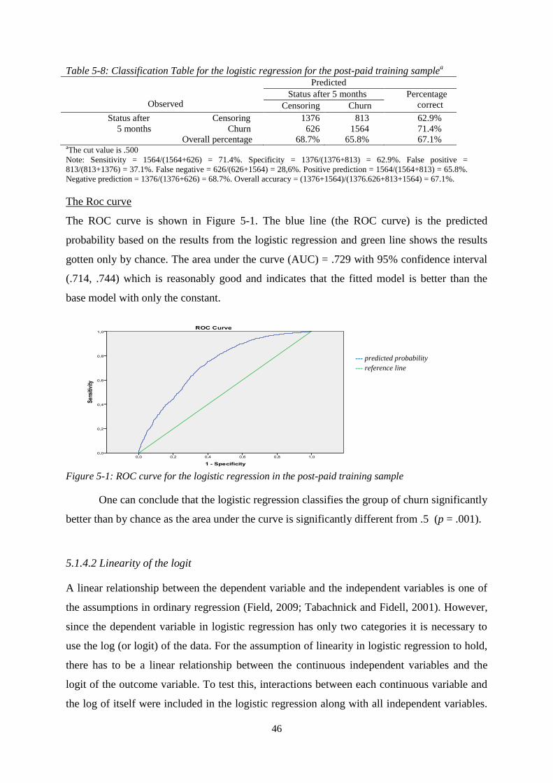
46
Table 5-8: Classification Table for the logistic regression for the post-paid training samplea
Observed
Predicted
Status after 5 months Percentage
correct Censoring Churn
Status after Censoring
5 months Churn
Overall percentage
1376
626
68.7%
813
1564
65.8%
62.9%
71.4%
67.1% aThe cut value is .500
Note: Sensitivity = 1564/(1564+626) = 71.4%. Specificity = 1376/(1376+813) = 62.9%. False positive =
813/(813+1376) = 37.1%. False negative = 626/(626+1564) = 28,6%. Positive prediction = 1564/(1564+813) = 65.8%.
Negative prediction = 1376/(1376+626) = 68.7%. Overall accuracy = (1376+1564)/(1376.626+813+1564) = 67.1%.
The Roc curve
The ROC curve is shown in Figure 5-1. The blue line (the ROC curve) is the predicted
probability based on the results from the logistic regression and green line shows the results
gotten only by chance. The area under the curve (AUC) = .729 with 95% confidence interval
(.714, .744) which is reasonably good and indicates that the fitted model is better than the
base model with only the constant.
--- predicted probability
--- reference line
Figure 5-1: ROC curve for the logistic regression in the post-paid training sample
One can conclude that the logistic regression classifies the group of churn significantly
better than by chance as the area under the curve is significantly different from .5 (p = .001).
5.1.4.2 Linearity of the logit
A linear relationship between the dependent variable and the independent variables is one of
the assumptions in ordinary regression (Field, 2009; Tabachnick and Fidell, 2001). However,
since the dependent variable in logistic regression has only two categories it is necessary to
use the log (or logit) of the data. For the assumption of linearity in logistic regression to hold,
there has to be a linear relationship between the continuous independent variables and the
logit of the outcome variable. To test this, interactions between each continuous variable and
the log of itself were included in the logistic regression along with all independent variables.

47
All the interactions terms were insignificant since their significant values were greater than
.05. This implies that the assumption of linearity of the logit has been met for the continuous
variables in the data (Field, 2009; Tabachnick and Fidell, 2001).
5.1.4.3 Validation
To validate the results of the logistic regression, the logistic model was tested on another
sample from Telecom X. The main difference with this sample is that it is not balanced like
the training sample. There are 28737 cases in this testing sample, 27910 active customers and
only 827 churners or 2.9%. This reflects the real life situation where the percentage of churn
is very low on a monthly basis. 46% of the sample are women, 96.6% pay the bill themselves
and 50% are light users. Similar to the training sample, most of the customers come from the
greater capital area or 55.2%, 14.5% come from the northern part of Iceland and the same
goes for southern Iceland. 8.8% come from the western part and 5.4% come from the eastern
part. This is very similar to the distribution in the training sample. 1.7% had an unknown
residency. The size of family was somewhat different as there were up to 11 people in a
family in the testing sample but up to 7 in the training sample. As with the training sample,
there are much fewer cases in each of the categories from 4 people to 11 people so a new
variable was made with 3 categories, 1 person, 2 people and 3 people or more, to make the
categories more similar in size. Finally, of the demographic variables, marital status was also
quite comparable with the training set. The category with married people was largest, or
54.6%. 25.9% were unmarried, 10.6% divorced, 6.1% widowed and 1.2% separated. Finally,
0.8% had another marital status than specified above. 207 or 0.7% had an unknown marital
status. The mean age was slightly higher in the testing sample or 52.26 years (SD = 15.03).
The youngest customers were 18 and the oldest was 101 years old. The mean for tenure was
1641.12 days (SD = 1563.95. The minimum number of days was 31 and the highest number
was 4544 or over 12 years. The average number of products was 27 compared to 29.8
products in the training sample. The mean for the average amount paid for mobile phone
usage over the three months in the testing sample is lower than in the training sample, or
8076.8 ISK and 9103.1 ISK respectively.
To test the resulting logistic regression model produced with the training sample,
scores are calculated in the testing data set based on the model. SPSS makes it possible to
export the model information to a new data set which is used for testing the model and
produces scores for each case in the new set. Those cases with a score > .5 were classified as

48
churn, those with a score <= .5 were classified as non-churn. The predicted status was then
compared with the actual status for each case. The results of the overall classification are
shown in Table 5-9.
Table 5-9: Classification table for the logistic regression for the post-paid testing samplea
Observed
Predicted
Status after 5 months Percentage
correct Censoring Churn
Status after Censoring
5 months Churn
Overall percentage
14739
137
99.1%
13171
690
5.0%
52.8%
83.4%
53.7% aThe cut value is .500
Note: Sensitivity = 690/(690+137) = 83.4%. Specificity = 14739/(14739+13171) = 52.8%. False positive =
13171/(13171+14,739) = 47.2%. False negative = 137/(137+690) = 16.6%. Positive prediction = 690/(690+13171) =
5.0%. Negative prediction = 14739/(14739+137) = 99.1%. Overall accuracy = (14739+690)/(14739+137+13171+690)
= 53.7%.
The model correctly predicted the status for churn in 690 cases or 83.4% of the 827
customers that actually churned. It did poorer at predicting for non-churn, as it had a
specificity of 52.8%. The false positive rate or Type I error was 47.2% as it predicted 13171
cases as churners which were actually still active. Finally, the false negative or Type II error
was relatively low, or 16.6% as it predicted 137 as non-churn who had actually churned. In
this case, it is better to have a lower Type II error since it is worse to misclassify someone
who churned as non-churn than to misclassify someone who is still active as churn. As a
result of the high number of false positives, the overall accuracy was 53.7% which is lower
than with the training sample of 67.1%. The model had a very low positive predictive value of
5.0% as it incorrectly predicted so many non-churn cases as churn. The negative predictive
value was particularly high or 99.1%.
5.1.5 Decision Tree
This procedure generates a model that is a tree-based classification model. What this model
does is to categorize cases into groups or it predicts values of a dependent variable based on
the independent variables’ values.
With large datasets, the speed of classification can decrease and the average depth of a
decision tree can get deeper. This means that the tree’s structure grows to be large and
complicated. By using the results from the PCA previously done, noise data can be filtered
and the dimensions of the data set are reduced (Hu et al., 2009). This was supported by a
research by Piramuthu (2008) where the results showed that when multicollinearity was
present in the data, reducing either the dimensionality or the size of the sample with factor

49
analysis or cluster analysis would improve the performance of the decision tree, both reducing
the size of the tree and decreasing the predicting error.
5.1.5.1 Results of the Decision Tree
As described in section 3.4.2, there are four growing methods that can be used. They were all
used in turn with the intention of comparing the results to see which is the best method. The
same 38 variables were used as in the logistic regression done previously.
The methods were used in the same order as they appear in section 3.4.2. CHAID
generated a decision tree with 35 nodes, 22 terminal nodes and a depth of 3, which specifies
the number of levels below the root node. Exhaustive CHAID generated a decision tree with
28 nodes, 18 terminal nodes and a depth of 3. CRT produced a tree with 19 nodes, 10 terminal
nodes and a depth of 5. Lastly, QUEST produced a tree with 31 nodes, 16 terminal nodes and
also a depth of 5. CHAID used nine of the 38 variables in the analysis to create a tree and
exhaustive CHAID included seven of the 38 variables used in the analysis, QUEST used 26
variables and CRT used all the variables except two, “Is payer” and “Gender”. Those
variables that did not make a significant contribution were dropped from the model. For the
methods CHAID, exhaustive CHAID and CRT, the variable “Average text messages in” was
the best predictor for customers’ status. With the QUEST method, customer age was the best
predictor.
CRT was the method that had the highest overall classification value of 67.6%.
Exhaustive CHAID had the second highest value of 67.1%, CHAID had 66.80% and QUEST
had 65.8%. However, exhaustive CHAID had the highest sensitivity of 77.8% which means
that it predicted churn correct in almost 78% of the cases and this is what the analysis is
focusing on. The second highest was QUEST with a sensitivity of 76.7%. CRT had 75.8%
and CHAID had 73.7%. CHAID had the highest specificity of 59.9% so it did best of the four
methods in predicting for non-churn. CRT had 59.5%, exhaustive CHAID 56.4% and QUEST
had 54.9%. Table 5-10 on the next page shows the risk estimate of the four different growing
methods and as can be seen, CRT had the lowest risk estimate of .324. It indicates that the
category that was predicted by the model (churn or non-churn) was wrong in 32.4% of the
cases. This means that the “risk” of misclassifying a customer is around 32%. QUEST had the
highest risk estimate of .342. All four methods had a standard error of .007.
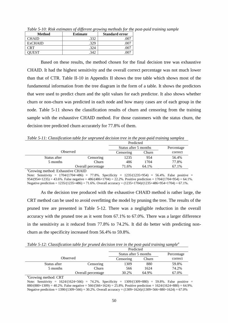
50
Table 5-10: Risk estimates of different growing methods for the post-paid training sample Method Estimate Standard error
CHAID .332 .007
ExCHAID .329 .007
CRT .324 .007
QUEST .342 .007
Based on these results, the method chosen for the final decision tree was exhaustive
CHAID. It had the highest sensitivity and the overall correct percentage was not much lower
than that of CTR. Table II-10 in Appendix II shows the tree table which shows most of the
fundamental information from the tree diagram in the form of a table. It shows the predictors
that were used to predict churn and the split values for each predictor. It also shows whether
churn or non-churn was predicted in each node and how many cases are of each group in the
node. Table 5-11 shows the classification results of churn and censoring from the training
sample with the exhaustive CHAID method. For those customers with the status churn, the
decision tree predicted churn accurately for 77.8% of them.
Table 5-11: Classification table for unpruned decision tree in the post-paid training samplea
Observed
Predicted
Status after 5 months Percentage
correct Censoring Churn
Status after Censoring
5 months Churn
Overall percentage
1235
486
71.6%
954
1704
64.1%
56.4%
77.8%
67.1% aGrowing method: Exhaustive CHAID
Note: Sensitivity = 1704/(1704+486) = 77.8%. Specificity = 1235/(1235+954) = 56.4%. False positive =
954/(954+1235) = 43.6%. False negative = 486/(486+1704) = 22.2%. Positive prediction = 1704/(1704+954) = 64.1%.
Negative prediction = 1235/(1235+486) = 71.6%. Overall accuracy = (1235+1704)/(1235+486+954+1704) = 67.1%.
As the decision tree produced with the exhaustive CHAID method is rather large, the
CRT method can be used to avoid overfitting the model by pruning the tree. The results of the
pruned tree are presented in Table 5-12. There was a negligible reduction in the overall
accuracy with the pruned tree as it went from 67.1% to 67.0%. There was a larger difference
in the sensitivity as it reduced from 77.8% to 74.2%. It did do better with predicting non-
churn as the specificity increased from 56.4% to 59.8%.
Table 5-12: Classification table for pruned decision tree in the post-paid training samplea
Observed
Predicted
Status after 5 months Percentage
correct Censoring Churn
Status after Censoring
5 months Churn
Overall percentage
1309
566
30.2%
880
1624
64.9%
59.8%
74.2%
67.0% aGrowing method: CRT
Note: Sensitivity = 1624/(1624+566) = 74.2%. Specificity = 1309/(1309+880) = 59.8%. False positive =
880/(880+1309) = 40.2%. False negative = 566/(566+1624) = 25.8%. Positive prediction = 1624/(1624+880) = 64.9%.
Negative prediction = 1390/(1309+566) = 30.2%. Overall accuracy = (1309+1624)/(1309+566+880+1624) = 67.0%

51
With the pruned tree, there was a minute increase in the risk estimate from .329 to
.330. This pruned model also predicted fewer churned customers correctly, or 1624, however
it predicted more non-churners correctly, or 1309. The difference can also be seen in the
model summary since the tree goes from having 19 nodes and 10 terminal nodes to having 9
nodes and 5 terminal nodes. The depth of the tree went from 5 to 4. The pruned tree table is
shown in Table II-11 and the tree diagram in Figure II-2 in Appendix II. “Average number of
text messages sent” is the best predictor in the decision tree. Also in the tree are “Tenure”,
“Customer age” and “Land area” which were significant in the logistic regression as well.
74.9% of the customers who sent less than 7.17 text messages over the three month period
were still active while 60.5% of the customers who send more than 7.17 text messages on
average over the three month period have churned. The next best predictor for those who sent
more than 7.17 messages was “Tenure” and for those who have stayed less than 1359.5 days,
68.5% of them had churned. Slightly more than half (53.5%) of those who have stayed longer,
churned. This shows that customers who have stayed longer are less likely to churn, which
concurs with the results from the logistic regression. For customers who have stayed longer
than 1359.5 days, 56.8% of those who are older than 53.5 years old are more likely to stay. Of
those who are younger than 53.5 years old, 58.3% of them have churned. So younger
customers are more likely to churn which is the same effect as in the logistic regression.
Finally, of those in the node with customers younger than 53.5 years old, 24.5% of them who
live in Eastern Iceland have churned. Of those in the other categories for “Land area”, 60%
have churned which was also the same as in the logistic regression. Over all, the same effects
apply for the variables that are significant in both classification methods.
Gain is calculated for each terminal node to show the node’s performance. Gain is the
percentage of total cases predicted for in the target category (in this case churn) in a terminal
node of the total cases of the target category in the whole sample. In this decision tree, node 2
has the highest gain of 85.2%. A gains chart plots the gain percent for the whole tree. The
gains chart is showed in Figure II-3 in Appendix II. It implies that the model is a moderately
good one. These cumulative charts always start at 0% and end at 100% as one goes from one
end to the other. For a good model, the line will rise steeply toward 100% and then level off.
A model that follows the diagonal reference line gives no information.

52
The ROC curve
The ROC curve for the decision tree is shown in Figure 5-2. AUC for the decision tree = .697
with 95% confidence interval (.681, .712) and a p = .001 so it is a statistical significant ROC
curve. AUC of .697 indicates that it is a fair test. The AUC is lower for the decision tree than
for the logistic regression, which was .729.
--- predicted probability --- reference line
Figure 5-2: ROC curve for the decision tree in the post-paid training sample
5.1.5.2 Validation
This procedure evaluates how well the tree structure generalizes to a larger population. To test
the decision tree model generated using the training sample, the decision tree diagram is
followed down and the cases in the testing sample labeled churn or non-churn according to
the probability of churn or non-churn in each terminal node. SPSS makes a score for each
case based on the decision tree model and those with a score > .5 are labeled as churn, those
with a score <= .5 are labeled as non-churn. This sample was described in section 5.1.4.3. The
results are shown in Table 5-13. As the table shows, the decision tree model predicted the
status correctly for 630 churners out of the 827, or 76.2% which is the sensitivity.
Table 5-13: Classification table for decision tree in the post-paid testing samplea
Observed
Predicted
Status after 5 months Percentage
correct Censoring Churn
Status after Censoring
5 months Churn
Overall percentage
16714
197
98.8%
11196
630
5.3%
59.9%
76.2%
60.4% aGrowing method: CRT
Note: Sensitivity = 630/(630+197) = 76.2%. Specificity = 16714/(16714+11196) = 59.9%. False positive =
11196/(11196+16714) = 40.1%. False negative = 197/(197+630) = 23.8%. Positive prediction = 630/(630+11196) =
5.3%. Negative prediction = 16714/(16714+197) = 98.8%. Overall accuracy =
(16714+630)/(16714+197+11196+630) = 60.4%.

53
The specificity was 59.9% meaning that the model predicts correctly for 60% of those
customers who did not churn. The false positive rate was high or 40.1% as the model
predicted many cases as churners which were in fact still active. This is the same as with the
logistic regression. The false negative rate was 23.8%. The overall accuracy was 60.4% which
is higher than with the logistic regression which had 53.7%. The positive predictive value was
extremely low at 5.0% as the model predicted so many cases incorrectly as churn. However,
the negative predictive value was 98.8%.
Based on the results from the validation of both the logistic regression and the decision
tree, it is difficult to see which method should be recommended for churn prediction. One
could make the deduction that the logistic regression would be more suitable of these two
classification methods. The overall accuracy is relatively lower for the testing sample with the
logistic regression but it had a higher sensitivity, therefore predicting churn more accurately
which is of main interest here. Otherwise, there is perhaps not a straightforward way to
compare these two classification methods as they differ in many ways. It seems that the
logistic regression is somewhat better at predicting churn and with this method, one can see
the size of the effect each significant variable has on churn and whether there is a positive or
negative relationship between the variables and churn. The decision tree on the other hand, is
convenient as the tree diagram can show how one choice leads to another as one follows
down the tree. The tree illustrates the relationship between different attributes (like gender,
tenure, usage and billing) and possible end results (churn or non-churn). Both methods
therefore have their own specific characteristics.
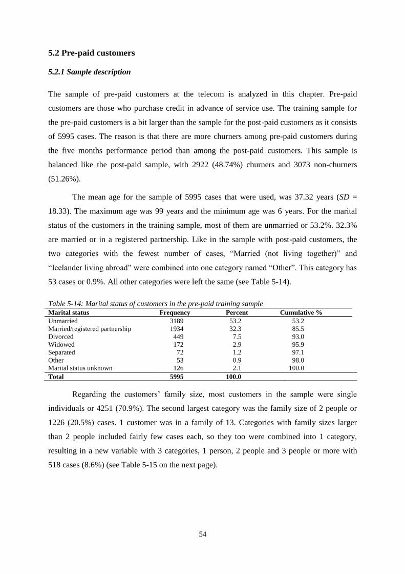
54
5.2 Pre-paid customers
5.2.1 Sample description
The sample of pre-paid customers at the telecom is analyzed in this chapter. Pre-paid
customers are those who purchase credit in advance of service use. The training sample for
the pre-paid customers is a bit larger than the sample for the post-paid customers as it consists
of 5995 cases. The reason is that there are more churners among pre-paid customers during
the five months performance period than among the post-paid customers. This sample is
balanced like the post-paid sample, with 2922 (48.74%) churners and 3073 non-churners
(51.26%).
The mean age for the sample of 5995 cases that were used, was 37.32 years (SD =
18.33). The maximum age was 99 years and the minimum age was 6 years. For the marital
status of the customers in the training sample, most of them are unmarried or 53.2%. 32.3%
are married or in a registered partnership. Like in the sample with post-paid customers, the
two categories with the fewest number of cases, “Married (not living together)” and
“Icelander living abroad” were combined into one category named “Other”. This category has
53 cases or 0.9%. All other categories were left the same (see Table 5-14).
Table 5-14: Marital status of customers in the pre-paid training sample
Marital status Frequency Percent Cumulative %
Unmarried 3189 53.2 53.2
Married/registered partnership 1934 32.3 85.5
Divorced 449 7.5 93.0
Widowed 172 2.9 95.9
Separated
Other
Marital status unknown
72
53
126
1.2
0.9
2.1
97.1
98.0
100.0
Total 5995 100.0
Regarding the customers’ family size, most customers in the sample were single
individuals or 4251 (70.9%). The second largest category was the family size of 2 people or
1226 (20.5%) cases. 1 customer was in a family of 13. Categories with family sizes larger
than 2 people included fairly few cases each, so they too were combined into 1 category,
resulting in a new variable with 3 categories, 1 person, 2 people and 3 people or more with
518 cases (8.6%) (see Table 5-15 on the next page).
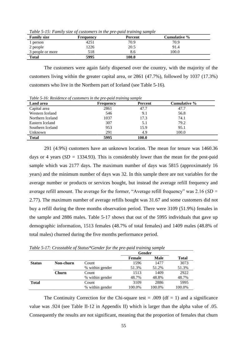
55
Table 5-15: Family size of customers in the pre-paid training sample
Family size Frequency Percent Cumulative %
1 person 4251 70.9 70.9
2 people 1226 20.5 91.4
3 people or more 518 8.6 100.0
Total 5995 100.0
The customers were again fairly dispersed over the country, with the majority of the
customers living within the greater capital area, or 2861 (47.7%), followed by 1037 (17.3%)
customers who live in the Northern part of Iceland (see Table 5-16).
Table 5-16: Residence of customers in the pre-paid training sample
Land area Frequency Percent Cumulative %
Capital area 2861 47.7 47.7
Western Iceland 546 9.1 56.8
Northern Iceland 1037 17.3 74.1
Eastern Iceland 307 5.1 79.2
Southern Iceland
Unknown
953
291
15.9
4.9
95.1
100.0
Total 5995 100.0
291 (4.9%) customers have an unknown location. The mean for tenure was 1460.36
days or 4 years (SD = 1334.93). This is considerably lower than the mean for the post-paid
sample which was 2177 days. The maximum number of days was 5815 (approximately 16
years) and the minimum number of days was 32. In this sample there are not variables for the
average number or products or services bought, but instead the average refill frequency and
average refill amount. The average for the former, “Average refill frequency” was 2.16 (SD =
2.77). The maximum number of average refills bought was 31.67 and some customers did not
buy a refill during the three months observation period. There were 3109 (51.9%) females in
the sample and 2886 males. Table 5-17 shows that out of the 5995 individuals that gave up
demographic information, 1513 females (48.7% of total females) and 1409 males (48.8% of
total males) churned during the five months performance period.
Table 5-17: Crosstable of Status*Gender for the pre-paid training sample Gender
Total Female Male
Status Non-churn Count 1596 1477 3073
% within gender 51.3% 51.2% 51.3%
Churn Count 1513 1409 2922
% within gender 48.7% 48.8% 48.7%
Total Count 3109 2886 5995
% within gender 100.0% 100.0% 100.0%
The Continuity Correction for the Chi-square test = .009 (df = 1) and a significance
value was .924 (see Table II-12 in Appendix II) which is larger than the alpha value of .05.
Consequently the results are not significant, meaning that the proportion of females that churn

56
is not significantly different from the proportion of males that churn. As with the post-paid
sample, the same test was done for family size, land area, marital status and total charge
groups. For “Family size” the Pearson Chi-square = 3.254 (df = 2) with a p = .197, thus there
is no difference in status and number of people in the family. For “Land area” the chi-square
= 132.934 (df = 5) and p = .001 so there was a difference in status and where people live. The
Cramer’s V = .149 suggesting a somewhat strong relationship. The Chi-square for “Marital
status” = 209.997 (df = 6) and a p = .001. So there is a difference between customer status and
family status and the Cramer’s V = .187 (p = .001) indicating a relatively strong relationship.
Finally, for the “Total charge groups” the Chi-square = 179.623 (df = 1) and p = .001. This
relationship is also significantly different and the Cramer’s V = .173 (p = .001). Since the
variable “Is payer” only has one category left (of two) after filtering out customers with no
demographic information, it was omitted from the analysis.
The next step was to discover if there was a significant difference in the mean of the
continuous variables and the customer status by doing an independent samples t-test. Out of
the 61 variables related to demographics, averages and maximum values, 48 were significant
with a p < .05 in the Levene’s test (see Table II-13 in Appendix II). For these variables, the
variance of scores for the two groups in customer status is not the same. The insignificant
variables in the Levene’s test were “Average innet frequency”, “Average total out volume”,
“Average abroad volume ratio”, “Average abroad frequency ratio”, “Average voice outin
volume ratio”, “Average innet charge”, “Average abroad total charge ratio”, “Maximum voice
outin volume ratio”, “Maximum innet frequency”, “Maximum total out volume”, “Maximum
outnet volume ratio”, “Maximum outnet frequency ratio” and “Maximum innet charge”. For
the t-test for equality of means, 19 variables were insignificant with a p > .05 showing that
there is not a significant difference in the mean values for the two groups for customer status.
They were “Maximum refill amount”, “Average innet volume”, “Average abroad volume”,
“Average innet volume ratio”, “Average innet frequency ratio”, “Average abroad volume
ratio”, “Average abroad frequency ratio”, “Average voice outin volume ratio”, “Average
abroad charge”, “Average abroad total charge ratio”, “Maximum voice outin volume ratio”,
“Maximum innet volume”, “Maximum abroad volume”, “Maximum innet volume ratio”,
“Maximum innet frequency ratio”, “Maximum abroad volume ratio”, “Maximum abroad
frequency ratio”, “Maximum abroad charge” and “Maximum abroad total charge ratio”.
Then to measure the effect size statistics, Eta squared was calculated (see equation 5-
1) and the values ranged from 7.58*10-6
to .0818 which is similar to the post-paid sample.

57
“Average outnet total charge ratio” had the highest eta and therefore 8.18% of the variance in
this variable is explained by customer status.
5.2.2 Multicollinearity
To check whether multicollinearity is an issue in the data, the tolerance and VIF (Variance
Inflation Factor) statistics were looked at. A total of 58 variables related to usage and charge
were entered into linear regression and all but 5 had a tolerance value < .1 and VIF > 10
revealing that there is an issue with multicollinearity in the data. The decision was taken to
run a principal component analysis on all 58 usage and charge variables.
5.2.3 Principal component analysis
To see if the 53 variables which were involved in the multicollinearity form coherent subsets,
a Principal component analysis (PCA) was performed.
The 58 items used in the PCA were related to usage and charges, both inside and
outside the telecom’s network as well as abroad (see Table II-14 in Appendix II). The values
for the KMO and Bartlett’s test with all items included were .796 and 779787.833
respectively and a significance of .001 (df = 1653) which confirmed the sampling adequacy
for the analysis. Only “Maximum refill amount” had an individual KMO value < .5 and was
removed. By doing so, the communality for “Average refill amount” became < .5 and was
also removed. After the removal of these two items, all other items in the analysis had an
individual KMO and communality > .5 which implied that they were all applicable for the
PCA. The number of eigenvalues > 1 suggested that 12 components would be an appropriate
solution and the scree plot showed a point of inflexion at 2, 4, 7, 8 and 17 implying a solution
with 1, 3, 6, 7 or 16 components (see Figure II-4 in Appendix II). The components were next
rotated with the Varimax rotation method. After removing the two items mentioned above, a
solution with 12 components was not appropriate anymore since one component only
consisted of very low loadings. A solution with 11 components was tried but still one
component had only low loadings so ten components were extracted. After omitting total of
six items based on low KMO values or low loadings (see Table II-15 in Appendix II), a
solution of ten components was the result.
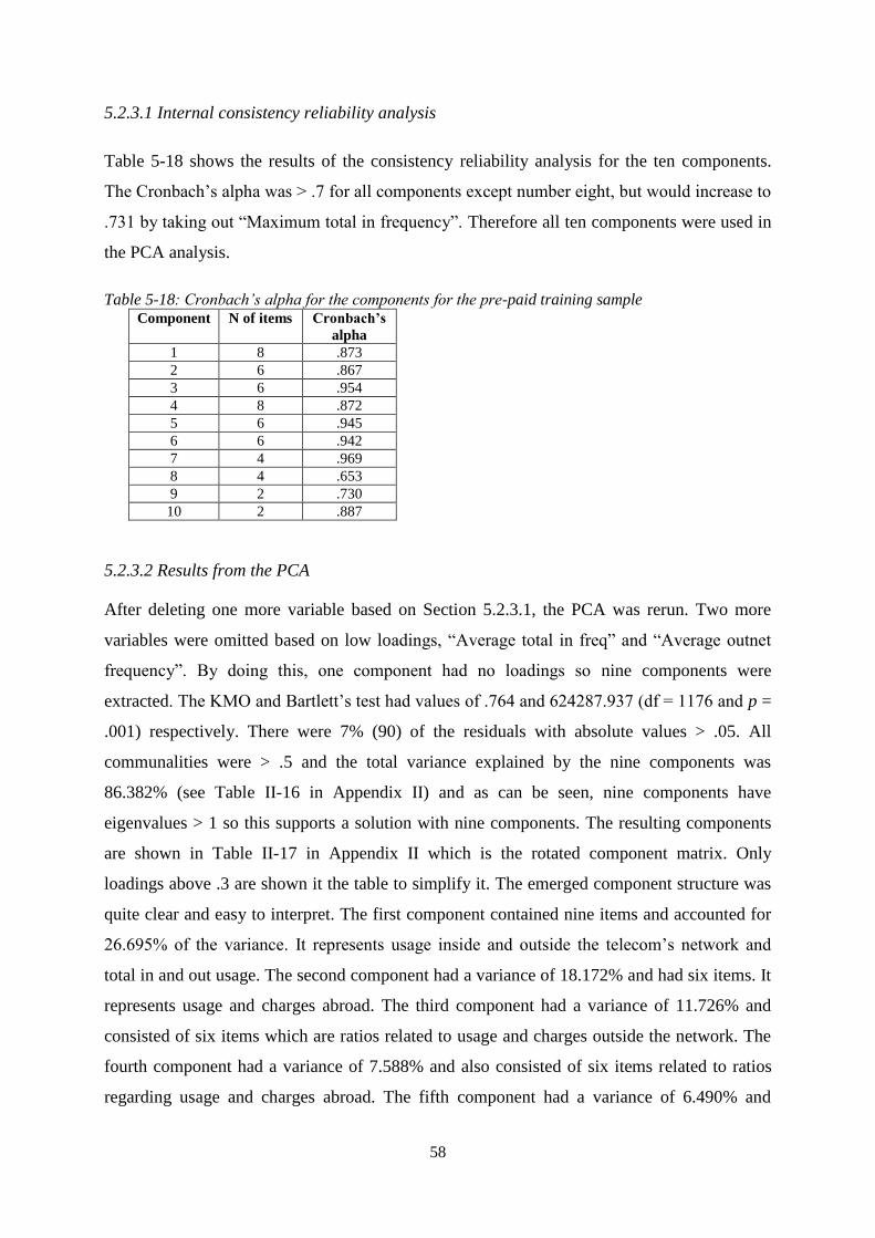
58
5.2.3.1 Internal consistency reliability analysis
Table 5-18 shows the results of the consistency reliability analysis for the ten components.
The Cronbach’s alpha was > .7 for all components except number eight, but would increase to
.731 by taking out “Maximum total in frequency”. Therefore all ten components were used in
the PCA analysis.
Table 5-18: Cronbach’s alpha for the components for the pre-paid training sample Component N of items Cronbach’s
alpha
1 8 .873
2 6 .867
3 6 .954
4 8 .872
5 6 .945
6 6 .942
7 4 .969
8 4 .653
9 2 .730
10 2 .887
5.2.3.2 Results from the PCA
After deleting one more variable based on Section 5.2.3.1, the PCA was rerun. Two more
variables were omitted based on low loadings, “Average total in freq” and “Average outnet
frequency”. By doing this, one component had no loadings so nine components were
extracted. The KMO and Bartlett’s test had values of .764 and 624287.937 (df = 1176 and p =
.001) respectively. There were 7% (90) of the residuals with absolute values > .05. All
communalities were > .5 and the total variance explained by the nine components was
86.382% (see Table II-16 in Appendix II) and as can be seen, nine components have
eigenvalues > 1 so this supports a solution with nine components. The resulting components
are shown in Table II-17 in Appendix II which is the rotated component matrix. Only
loadings above .3 are shown it the table to simplify it. The emerged component structure was
quite clear and easy to interpret. The first component contained nine items and accounted for
26.695% of the variance. It represents usage inside and outside the telecom’s network and
total in and out usage. The second component had a variance of 18.172% and had six items. It
represents usage and charges abroad. The third component had a variance of 11.726% and
consisted of six items which are ratios related to usage and charges outside the network. The
fourth component had a variance of 7.588% and also consisted of six items related to ratios
regarding usage and charges abroad. The fifth component had a variance of 6.490% and

59
consisted of eight items related to charges inside and outside the network along with
frequency of refills. The sixth component had a variance of 5.327% and consisted of six items
related to rations with usage and charge inside the network. The seventh component had a
variance of 3.890% and consisted of four items related to sent and received text messages.
The eighth component had a variance of 3.434% and consists of two items, average and
maximum voice outin volume ratio. The ninth and last component had a variance of 3.061%
and had two items, average and maximum ratios for sent text messages related to text
messages received. The following description of the nine components is based on the items in
each of them:
Component 1: Usage inside and outside the telecom’s network
Component 2: Usage/charges abroad
Component 3: Usage/charge ratios outside telecom’s network
Component 4: Usage/charge ratios abroad
Component 5: Refills and charges inside and outside the telecom’s network
Component 6: Usage/charge ratios inside the telecom’s network
Component 7: Text messages sent and received
Component 8: Ratio of voice volume out/in
Component 9: Ratio of sent and received text messages
5.2.3.3 Parallel analysis
Parallel analysis (PA) was used again as a technique to generate random variables to
determine the number of retained components to compare with the PCA results. The results
from the PA are shown in Table 5-19. This table shows that for the first nine components, the
eigenvalues are larger from the principal component analysis (PCA eigenvalue) but at the
tenth component, the eigenvalues from the parallel analysis (PA eigenvalue) become larger.
These results suggest that a nine component solution would be appropriate supporting the
previous results from the PCA.
Table 5-19: Comparison of PCA and PA eigenvalues for the pre-paid training sample
Component PCA eigenvalue PA eigenvalue
1 13.080 1.191
2 8.904 1.171
3 5.746 1.158
4 3.718 1.146
5 3.180 1.137
6 2.610 1.128
7 1.906 1.120
8 1.683 1.116
9 1.500 1.104
10 .966 1.097
*
.
49
.
.
.001
.
.
.850
*A number of components have been omitted from the table to save space
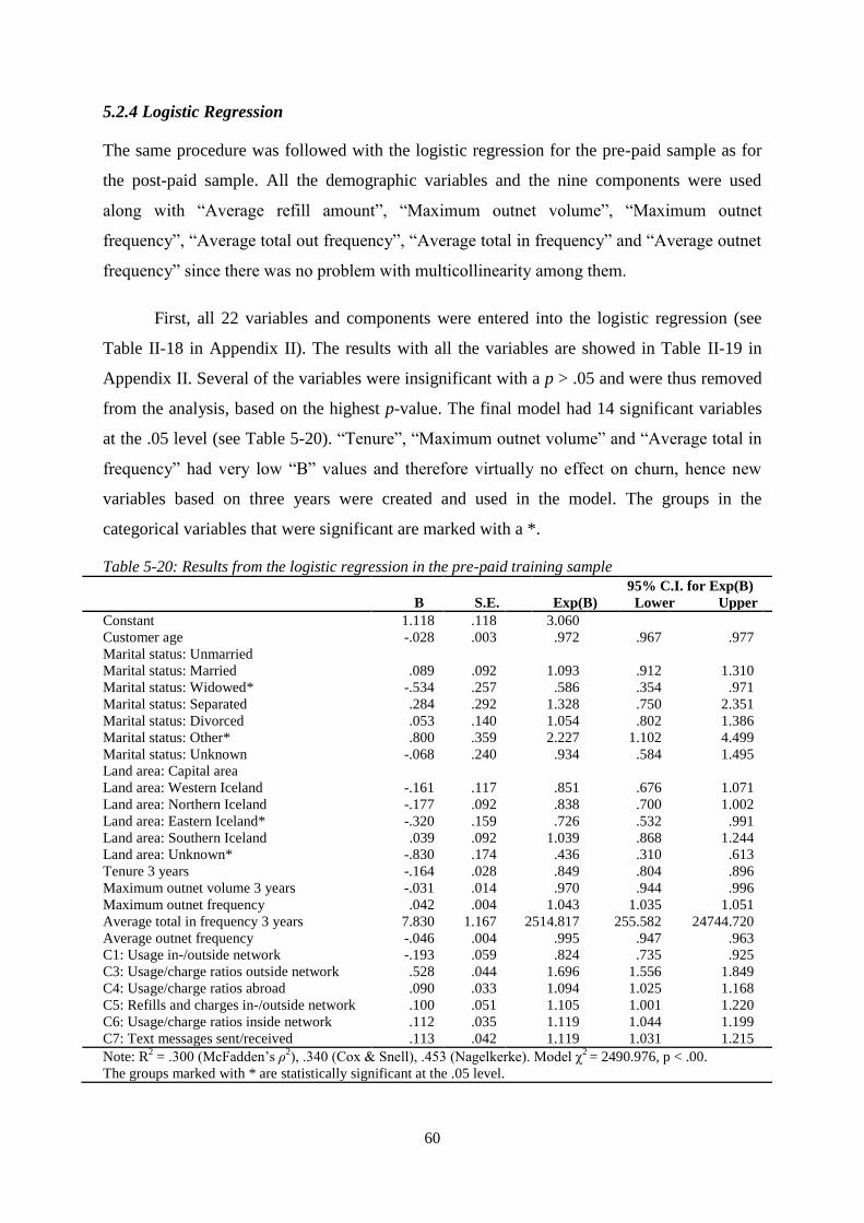
60
5.2.4 Logistic Regression
The same procedure was followed with the logistic regression for the pre-paid sample as for
the post-paid sample. All the demographic variables and the nine components were used
along with “Average refill amount”, “Maximum outnet volume”, “Maximum outnet
frequency”, “Average total out frequency”, “Average total in frequency” and “Average outnet
frequency” since there was no problem with multicollinearity among them.
First, all 22 variables and components were entered into the logistic regression (see
Table II-18 in Appendix II). The results with all the variables are showed in Table II-19 in
Appendix II. Several of the variables were insignificant with a p > .05 and were thus removed
from the analysis, based on the highest p-value. The final model had 14 significant variables
at the .05 level (see Table 5-20). “Tenure”, “Maximum outnet volume” and “Average total in
frequency” had very low “B” values and therefore virtually no effect on churn, hence new
variables based on three years were created and used in the model. The groups in the
categorical variables that were significant are marked with a *.
Table 5-20: Results from the logistic regression in the pre-paid training sample
B
S.E.
Exp(B)
95% C.I. for Exp(B)
Lower Upper
Constant
Customer age
Marital status: Unmarried
Marital status: Married
Marital status: Widowed*
Marital status: Separated
Marital status: Divorced
Marital status: Other*
Marital status: Unknown
1.118
-.028
.089
-.534
.284
.053
.800
-.068
.118
.003
.092
.257
.292
.140
.359
.240
3.060
.972
1.093
.586
1.328
1.054
2.227
.934
.967
.912
.354
.750
.802
1.102
.584
.977
1.310
.971
2.351
1.386
4.499
1.495
Land area: Capital area
Land area: Western Iceland
Land area: Northern Iceland
-.161
-.177
.117
.092
.851
.838
.676
.700
1.071
1.002
Land area: Eastern Iceland* -.320 .159 .726 .532 .991
Land area: Southern Iceland .039 .092 1.039 .868 1.244
Land area: Unknown*
Tenure 3 years
Maximum outnet volume 3 years
Maximum outnet frequency
Average total in frequency 3 years
Average outnet frequency
C1: Usage in-/outside network
C3: Usage/charge ratios outside network
C4: Usage/charge ratios abroad
C5: Refills and charges in-/outside network
C6: Usage/charge ratios inside network
C7: Text messages sent/received
-.830
-.164
-.031
.042
7.830
-.046
-.193
.528
.090
.100
.112
.113
.174
.028
.014
.004
1.167
.004
.059
.044
.033
.051
.035
.042
.436
.849
.970
1.043
2514.817
.995
.824
1.696
1.094
1.105
1.119
1.119
.310
.804
.944
1.035
255.582
.947
.735
1.556
1.025
1.001
1.044
1.031
.613
.896
.996
1.051
24744.720
.963
.925
1.849
1.168
1.220
1.199
1.215
Note: R2 = .300 (McFadden’s ρ
2), .340 (Cox & Snell), .453 (Nagelkerke). Model χ
2 = 2490.976, p < .00.
The groups marked with * are statistically significant at the .05 level.

61
The value for Cox & Snell was .340 and for Nagelkerke it was .453. McFadden’s ρ2
was .3. The baseline model, including only the constant, had a -2Log likelihood of 8307.031.
The model was significant with a chi-square of 2490.976 (df = 23, p = .001) and the -2Log-
likelihood had decreased to 5816.054 which shows that including the variables improve the
model. The Hosmer and Lemeshow test was insignificant with a p = .435 indicating a good
model fit.
5.1.4.1 Results of logistic regression
The results from the logistic regression show that for the first variable “Customer age”, as the
age of a customer increases by one year, he or she is .97 less times likely to churn, with other
factors controlled. Customer age had the least effect on churn. This means that the older the
customers get, the likelihood that they churn decreases. For the variable “Marital status”,
groups 3 and 6 were significant. This implies that customers who are widowed are .59 times
less likely to churn than customers living alone but those with the marital status “Other” are
2.23 times more likely to churn than those living alone. For “Land area”, groups 4 and 6 were
significant, so those customers who live in the Eastern part of Iceland or have an unknown
address are .73 and .44 times (respectively) less likely to churn to those who live in the base
area, which is the capital area. The same procedure was done with the variable “Tenure” here
as in the post-paid sample, a new variable was computed based on 3 years to get a better
indication of the effect of this variable on churn. Customers are .85 times less likely to churn
as tenure increases by 3 years. This shows that as a customer stays longer, the less likely he or
she is in churning.
The next variable in the table is “Maximum outnet volume”, based on three years. As
this variable increases by one unit, the likelihood that the customer will churn is .970 times
less. The next variable is “Maximum outnet frequency”. For every 1 unit increase in this
variable, the likelihood of churn is 1.043 times more likely. As “Average total in frequency”,
also based on three years because of low “B” value, increases by one unit, a customer is
2514.82 times likelier to churn. This variable had by far the largest effect on churn with a “B”
value of 7.830. As “Average outnet frequency” increases by one unit, a customer is .955 times
less likely to churn. The first of the components that was significant was Component 1:
Usage in-/outside the telecom’s network. This is the only component which had a negative
effect on churn, when it increases by one unit, customers are .824 times less likely to churn.
As Component 3: Usage/charge ratios outside the network increases by one unit, customers
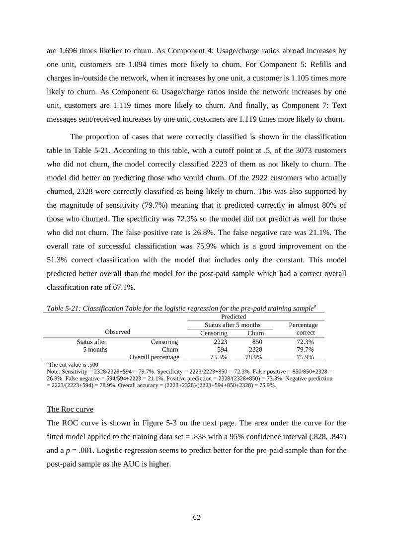
62
are 1.696 times likelier to churn. As Component 4: Usage/charge ratios abroad increases by
one unit, customers are 1.094 times more likely to churn. For Component 5: Refills and
charges in-/outside the network, when it increases by one unit, a customer is 1.105 times more
likely to churn. As Component 6: Usage/charge ratios inside the network increases by one
unit, customers are 1.119 times more likely to churn. And finally, as Component 7: Text
messages sent/received increases by one unit, customers are 1.119 times more likely to churn.
The proportion of cases that were correctly classified is shown in the classification
table in Table 5-21. According to this table, with a cutoff point at .5, of the 3073 customers
who did not churn, the model correctly classified 2223 of them as not likely to churn. The
model did better on predicting those who would churn. Of the 2922 customers who actually
churned, 2328 were correctly classified as being likely to churn. This was also supported by
the magnitude of sensitivity (79.7%) meaning that it predicted correctly in almost 80% of
those who churned. The specificity was 72.3% so the model did not predict as well for those
who did not churn. The false positive rate is 26.8%. The false negative rate was 21.1%. The
overall rate of successful classification was 75.9% which is a good improvement on the
51.3% correct classification with the model that includes only the constant. This model
predicted better overall than the model for the post-paid sample which had a correct overall
classification rate of 67.1%.
Table 5-21: Classification Table for the logistic regression for the pre-paid training samplea
Observed
Predicted
Status after 5 months Percentage
correct Censoring Churn
Status after Censoring
5 months Churn
Overall percentage
2223
594
73.3%
850
2328
78.9%
72.3%
79.7%
75.9% aThe cut value is .500
Note: Sensitivity = 2328/2328+594 = 79.7%. Specificity = 2223/2223+850 = 72.3%. False positive = 850/850+2328 =
26.8%. False negative = 594/594+2223 = 21.1%. Positive prediction = 2328/(2328+850) = 73.3%. Negative prediction
= 2223/(2223+594) = 78.9%. Overall accuracy = (2223+2328)/(2223+594+850+2328) = 75.9%.
The Roc curve
The ROC curve is shown in Figure 5-3 on the next page. The area under the curve for the
fitted model applied to the training data set = .838 with a 95% confidence interval (.828, .847)
and a p = .001. Logistic regression seems to predict better for the pre-paid sample than for the
post-paid sample as the AUC is higher.
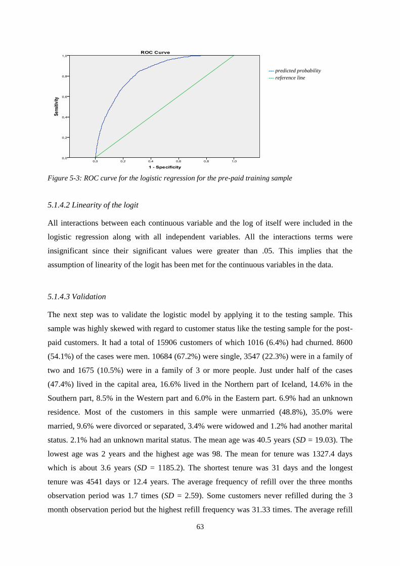
63
--- predicted probability
--- reference line
Figure 5-3: ROC curve for the logistic regression for the pre-paid training sample
5.1.4.2 Linearity of the logit
All interactions between each continuous variable and the log of itself were included in the
logistic regression along with all independent variables. All the interactions terms were
insignificant since their significant values were greater than .05. This implies that the
assumption of linearity of the logit has been met for the continuous variables in the data.
5.1.4.3 Validation
The next step was to validate the logistic model by applying it to the testing sample. This
sample was highly skewed with regard to customer status like the testing sample for the post-
paid customers. It had a total of 15906 customers of which 1016 (6.4%) had churned. 8600
(54.1%) of the cases were men. 10684 (67.2%) were single, 3547 (22.3%) were in a family of
two and 1675 (10.5%) were in a family of 3 or more people. Just under half of the cases
(47.4%) lived in the capital area, 16.6% lived in the Northern part of Iceland, 14.6% in the
Southern part, 8.5% in the Western part and 6.0% in the Eastern part. 6.9% had an unknown
residence. Most of the customers in this sample were unmarried (48.8%), 35.0% were
married, 9.6% were divorced or separated, 3.4% were widowed and 1.2% had another marital
status. 2.1% had an unknown marital status. The mean age was 40.5 years (SD = 19.03). The
lowest age was 2 years and the highest age was 98. The mean for tenure was 1327.4 days
which is about 3.6 years (SD = 1185.2). The shortest tenure was 31 days and the longest
tenure was 4541 days or 12.4 years. The average frequency of refill over the three months
observation period was 1.7 times (SD = 2.59). Some customers never refilled during the 3
month observation period but the highest refill frequency was 31.33 times. The average refill

64
amount was ISK 1805.62 (SD = 23010.1). The lowest amount was ISK 0.00 since some
customers never refilled and the highest amount was ISK 2508149.8.
To test the logistic model that was created using the training sample and see how well
it predicts for new cases, SPSS created scores in the testing dataset based on the logistic
regression model. Cases with a score (predicted probability) > .5 were labeled as churn, others
as non-churn. The results of the overall classification are shown in Table 5-22.
Table 5-22: Classification table for the logistic regression for the pre-paid testing samplea
Observed
Predicted
Status after 5 months Percentage
correct Censoring Churn
Status after Censoring
5 months Churn
Overall percentage
7689
179
97.7%
7201
837
10.4%
51.6%
82.3%
53.6% a. The cut value is .500
Note: Sensitivity = 837/(837+179) = 82.3%. Specificity = 7689/(7689+7201) = 51.6%. False positive =
7201/(7201+837) = 89.6%. False negative = 179/(179+7689) = 2.3%. Positive prediction = 837/(837+7201) = 10.4%.
Negative prediction = 7689/(7689+179) = 97.7%. Overall accuracy = (7689+837)/(7689+179+7201+837) = 53.6%.
The sensitivity was 82.3% which is higher than with the training sample which had
79.7%. The specificity was 51.6% which is quite lower than with the training sample which
had 72.3% so the model only predicts correctly for just over 51% of the cases for non-churn.
The false positive rate was very high or 89.6% which reflects the fact that the model predicts
so many cases as churn which are in fact non-churn. The false negative rate was on the
opposite very low, or 2.3%. The overall accuracy of the model is 53.6% which is much lower
than the 75.9% for the training sample and not much better than a model based only on
chance. In conclusion, this shows that the model does well when predicting for churn which is
the purpose of the model in this analysis but works rather poorly when predicting for non-
churn and has a high false positive rate.
5.1.5 Decision Tree
In this section, a tree-based classification model is produced the same way as the decision tree
model for the post-paid sample was made. The results are presented in the following section.
5.1.5.1 Results of Decision Tree
The same 22 variables were used to create the decision tree as in the logistic regression
analysis. The CHAID method produced a tree with 52 nodes, 34 terminal nodes and a depth

65
of 3. Ten variables were included in the model. The Exhaustive CHAID method produced a
tree with 51 nodes, 32 terminal nodes and a depth of 3 like CHAID. This method used 11
variables in the model. The CRT method produced a tree with much fewer nodes, or 25 and
13 terminal nodes. The depth was 5 (7, 4 and 3 respectively with pruning). It used all
variables for the model except “Gender”. The last method used in this analysis, QUEST,
yielded a tree with 29 nodes, 15 terminal nodes and a depth of 5 (15, 8 and 4 respectively with
pruning). It used 18 variables in the model. All methods had “Average outnet frequency” as
the primary predictor, except QUEST which had “Customer age” as the primary predictor.
Exhaustive CHAID had the highest overall classification percentage of 75.4% which is
quite higher than the highest overall percentage for the post-paid sample of 67.6%. CHAID
had a value of 75.3%. CRT had a slightly lower value of 73.9% and QUEST had the lowest
percentage of 70.6%. Table 5-23 shows the four methods’ risk estimate and it illustrates that
Exhaustive CHAID had the lowest estimate of .244 indicating that the models misclassified in
24.4% of the cases.
Table 5-23: Risk estimates of different growing methods for the pre-paid training sample Method Estimate Standard error
CHAID .247 .006
ExCHAID .244 .006
CRT .256 .006
QUEST .289 .006
Based on these results and the fact that Exhaustive CHAID had a correct prediction of
83.6% for churn but CHAID an 82.5%, Exhaustive CHAID was chosen as the best method in
this instance. The tree diagram is showed in Figure II-5 in Appendix II, but this is a pruned
tree with the CRT method as the tree diagram with the Exhaustive CHAID is very large and
more complicated to read through. The classification is showed in Table 5-24. The sensitivity
was, as already stated, 83.6% and the specificity was 67.7%. False positives were 28.1% and
false negatives were 19.7%.
Table 5-24: Classification table for the unpruned decision tree for pre-paid training samplea
Observed
Predicted
Status after 5 months Percentage
correct Censoring Churn
Status after Censoring
5 months Churn
Overall percentage
2134
522
80.3%
939
2400
71.9%
67.7%
83.6%
75.6% aGrowing method: Exhaustive CHAID
Note: Sensitivity = 2400/(2400+522) = 82.1%. Specificity = 2134/(2134+939) = 69.4%. False positive =
939/(939+2400) = 28.1%. False negative = 522/(522+2134) = 19.7%. Positive prediction = 2400/(2400+939) = 71.9%.
Negative prediction = 2134/(2134+522) = 80.3%. Overall accuracy = (2134+2400)/(2134+522+939+2400) = 75.6%.

66
The tree table is shown in Table II-20 in Appendix II. As can be seen, this table is
quite larger than for the post-paid training sample, and as in that case, the tree could be pruned
with the CRT growing method. Table II-21 in Appendix II show the pruned tree table and
Table 5-25 shows the overall classification with the pruned tree model. The overall correct
classification is now 73.9% and the sensitivity is 79.2% and specificity is 68.8%
Table 5-25: Classification table for the pruned decision tree for pre-paid training samplea
Observed
Predicted
Status after 5 months Percentage
correct Censoring Churn
Status after Censoring
5 months Churn
Overall percentage
2115
607
77.7%
958
2315
70.7%
68.8%
79.2%
73.9% aGrowing method: CRT
Note: Sensitivity = 2315/(2315+607) = 79.2%. Specificity = 2115/(2115+958) = 68.8%. False positive =
958/(958+2115) = 31.2%. False negative = 607/(607+2315) = 20.8%. Positive prediction = 2315/(2315+958) = 70.7%.
Negative prediction = 2115/(2115+607) = 77.7%. Overall accuracy = (2115+2315)/(2115+607+958+2315) = 73.9%.
“Average outnet frequency” was the best predictor for customer status as it is in node
1. The tree diagram with the Exhaustive CHAID method was very large and difficult to
follow so a pruned tree with CRT growing method is shown in Figure II-5 in Appendix II.
This diagram is much clearer and easier to follow. For customers who made more than 182.75
calls outside the telecom’s network, only 1.9% of them churned. This corresponds with the
results from the logistic regression. Slightly more than half of those who made less than
182.75 outside calls churned. Of those in the latter category, those who had “Average totalin
frequency” lower than 8.42, 26.7% churned. Of those with higher “Average totalin
frequency” than 8.42, 66.6% churned which is the same effect as with the logistic regression.
The last predictor in the tree was “Customer age”. 70.7% of those who are 55.5 years or
younger churn and 37.1% of those who are older than 55.5 years. This also corresponds with
the results from the logistic regression.
The gains chart shown in Figure II-6 in Appendix II illustrates that the model is a
moderately good one.
The ROC curve
The ROC curve for the decision tree is shown in Figure 5-4 on the next page. AUC for the
decision tree = .834 with a 95% confidence interval (.824, .844) and a p-value = .001.

67
--- predicted probability
--- reference line
Figure 5-4: ROC curve for the decision tree for the pre-paid training sample
5.1.5.2 Validation
To validate the decision tree model that resulted from the training data set, the pruned tree
diagram (in Figure II-5 in Appendix II) was used to make a prediction for the cases in the
testing sample for which SPSS produced scores based on the tree model. The results are
shown in the classification table in Table 5-26. As the table shows, the sensitivity was lower
using the decision tree than the logistic regression, or 77.5%. The specificity however was
higher than with the logistic regression, or 55.1%. The false positive rate was 44.9% and the
false negative rate was 22.5%. The overall accuracy was only 56.5% which is lower than with
the training sample which had 73.9% and not much better than a model based only on chance
which has an overall accuracy of 50%. The decision tree does slightly better than the logistic
regression which had an overall accuracy of 53.6%.
Table 5-26: Classification table for the decision tree in the pre-paid testing sample a
Observed
Predicted
Status after 5 months Percentage
correct Censoring Churn
Status after Censoring
5 months Churn
Overall percentage
8197
229
97.3%
6693
787
10.5%
55.1%
77.5%
56.5% aThe cut value is .500
Note: Sensitivity = 787/(787+229) = 77.5%. Specificity = 8197/(8197+6693) = 55.1%. False positive =
6693/(6693+8197) = 44.9%. False negative = 229/(229+787) = 22.5%. Positive prediction = 787/(787+6693) = 10.5%.
Negative prediction = 8197/(8197+229) = 97.3%. Overall accuracy = (8197+787)/(8197+229+6693+787) = 56.5%.

68
Based on the results from both classification methods on the testing sample, logistic
regression is more preferable. It does have a slightly lower sensitivity than the decision tree,
but it does have a higher sensitivity, therefore being better at predicting churn.
5.3 Hypotheses
Regarding the hypotheses stated in Section 2.2.3.1, the results of the logistic regression and
the decision tree show that for:
H1: Customer tenure
(a) Post-paid customers: As tenure was significant in both the logistic regression model
and the decision tree for the post-paid training sample, it has an effect on churn
probability. It had a negative “B” value in the logistic regression model and with the
decision tree, almost 70% of those with lower tenure had churned, therefore as a
customer stays longer with the telecom, the less likely they are to churn. Hence this
hypothesis is supported.
(b) Pre-paid customers: Tenure was also significant in the pre-paid sample in both the
logistic regression and the unpruned decision tree. It had a negative “B” value in the
logistic regression so it does have a negative effect on churn. This is also the case with
the decision tree as those who have been with the telecom for a shorter time are more
likely to churn. This part of the hypothesis is supported.
H2: Level of usage
(a) Post-paid customers: The usage factors did have some effect on customer churn in the
post-paid sample as the variables “Average abroad total charge ratio” and “Maximum
text messages outnet total charge ratio” along with components 1, 2 and 3 which are
composed of usage and charges inside and outside the telecom’s network and abroad,
were significant. These variables had a positive “B” value so as their values increase,
the customers are more likely to churn. For “Total charge groups” used in the logistic
regression, heavy users were more likely to churn. “Average text messages in” was
significant in the decision tree and more messages received was related to churn. Thus
this hypothesis is supported. However, component 4 (related to usage ratios abroad)
had a negative “B” value in the logistic regression meaning that as it increases, the
customer is less likely to churn. Consequently, these hypotheses are partly supported.

69
(b) Pre-paid customers: The same holds for influence of usage and charges on customer
churn in the pre-paid sample. Four independent variables were significant along with
six components which contain items of both usage and charges. However three of
these variables have a negative “B” value thus having a negative effect on churn. As
they increase by one unit, likelihood of churn decreases. For the remaining variables,
the “B” value was positive meaning that as they increase by one unit, the likelihood of
customer churn increases. For “Average outnet frequency” in the decision tree, the
more customers call outside the network, the less likely they are to churn, which is
opposite to the hypothesis. However, as the “Average totalin frequency” increases,
customers are more likely to churn. As a result, this hypothesis is partly supported.
H3: Customer age
(a) Post-paid customers: Customer age was significant in both classification models and
the “B” value in the logistic regression was negative, meaning that as the customers
get older, they are less likely to churn. The same holds for the decision tree and thus
this hypothesis is supported.
(b) Pre-paid customers: Customer age was also significant in the pre-paid sample in both
the logistic regression and the decision tree and had a negative “B” value in the
logistic regression and in the decision tree, those in the category with lower age are
more likely to churn so this hypothesis is also supported.
5.4 CLV calculations
In this section, model equation (2-1) was used to calculate the customer lifetime value for
each customer. The margin in the formula is the same as ARPU (see Section 2.2.1.1) and the
discount rate was discussed in Section 2.2.2.2 (see equation (2-2)). The third and last element
of the CLV model is the retention rate or 1-customer churn. The predicted probabilities for
churn for post- and pre-paid customers based on the logistic regression resulting from the
churn analysis in Sections 5.1 and 5.2 were used.
5.4.1 Segmentation
The customers in both the post-paid and pre-paid samples were segmented by ranking the
cases into 10 equal deciles based on the CLV values. The purpose of doing this is that
Telecom X can see what characterizes the customers in the top 10% decile from the other

70
deciles since these would be the customers who are most valuable to the company. When
these valuable customers are related with a high probability of churn, the company could try
to act on it by offering them something that might reduce the probability of churn. Telecom X
can also look at the other segments and see for example which customers have low CLV and
high probability of churn and then know that it would not be worth it spending marketing
resources trying to retain them.
Post-paid customers
The means for the CLV in the ten different segments are showed in Table II-22 in Appendix
II which is the result of One-way ANOVA. Segment 10 has the top 10% most valuable
customers and segment 1 has the bottom 10% least valuable customers. The ANOVA test (F
= 5503.97, p = .000) implies that there is a difference in the mean of CLV and the different
segments (see Table II-23 in Appendix II). There is a statistically significant difference
between all the segments except segment 1 and 2.
To find out if there was a difference between the ten segments and the demographic
characteristics, crosstables and One-Way ANOVA were conducted. This revealed a
statistically significant difference between the ten segments and all the demographic
variables. However the differences were not that large between segments. The customers in
the highest segments also have the highest average tenure. Overall this segmentation reveals
that there is a clear difference between segments 1 and 10 but the difference in the segments
in between these two is not as clear.
Pre-paid customers
The same procedure was used for the combined sample of pre-paid customers. However, only
nine ranks or segments were created as 22.9% of the sample had a CLV of 0.00.
Crosstabs and One-Way ANOVA were again conducted to see if there was a
difference between the ten segments and any of the demographic. All the tests were
statistically significant so there is a difference between the segments as with the post-paid
sample. However the difference is not always big. Customers in the lower segments are
younger than those in the higher segments. The higher segments also make more frequent
refills and for higher amounts. Finally, the customers in the higher segments have been with
the telecom longer than those in the lower segments. The same holds for this segmentation as
with the combined post-paid sample, the difference between the segments in between
segments 2 and 10 are not very clear.

71
5.5 Summary
In this chapter, the results of the thesis have been presented and discussed in detail.
Logistic regression and decision tree are two classification methods that have been
used frequently in research regarding churn. They are generally considered reliable and give
good prediction. Here, they have both been used and their results compared, for post-paid
customers and pre-paid customers.
There are a couple of factors which influence customer churn, both demographic and
the ones related to customer usage of mobile phone and the charges for that usage. The
influence has both a positive and negative effect. As one can imagine beforehand, as usage
increases, the charges increase and that has an increasing effect on churn. Age and tenure
however have a negative effect, so as they increase, a customer is less likely to churn. One
can conclude that older customers are more loyal to their telecom but younger customers
could also be more prone to changes and follow novelties and better deals. Tenure is also
associated with loyalty, those who have been with the telecom for a long time, are less likely
to churn. They clearly like what they are getting at the telecom but it could also mean that if
these customers buy other products and services at Telecom X it might be more difficult for
them to churn. Of the total of 33116 customers in the combined post-paid sample, 3017
(9.1%) had churned during the five month performance period while among the 21901
customers in the combined pre-paid sample, 3938 (18.0%) had churned. This is a large
difference which could be due to the fact that it is easier to cancel a pre-paid subscription than
a post-paid subscription.
For the post-paid training sample, both classification methods had almost the same
result in overall classification as the logistic regression had a 67.1% and the decision tree had
67.0% (pruned tree). The decision tree did better at predicting churn as it predicted correct in
74.2% of the cases while the logistic regression in 71.4% in the training sample. The
classifiers did better however with the pre-paid training sample. The logistic regression had a
75.9% overall classification correct and the decision tree a 75.4%, so there was not much
difference between the two methods. The decision tree did better again with predicting churn,
with a correct prediction in 82.5% of the cases but the logistic regression had 79.7% correct.
Customer lifetime value was calculated for the post-paid and pre-paid samples and it
showed that it can be a quite straightforward procedure, the most complicated element of it
however is predicting churn. There was a statistically significant difference between some of

72
the independent variables and CLV and it can be helpful to see where the difference lies. The
samples were then segmented based on the CLVs and the top 10% and bottom 10% deciles
were described to show the difference and that the segmentation can be used to identify
valuable customers in danger of churning.

73
6. Conclusion and recommendations
The results of the analysis for churn are in accordance with the literature related to churn as
the hypotheses were for the most part supported. For the post-paid customers, “Customer
age”, “Tenure” and “Land area” were the predictors chosen by both classification methods
indicating the importance of these predictors. If the information from the unpruned decision
tree is taken into account, components 2 and 3 are also chosen in both methods revealing that
usage and charge ratios both inside and outside the telecom’s network have an effect on churn
probability. For the pre-paid customers, “Customer age” along with “Average outnet
frequency” and “Average totalin frequency” were chosen by both classification methods.
However if the unpruned decision tree is used, “Tenure”, “Family size”, “Marital status”,
“Average refill amount”, “Maximum outnet frequency” and components 5 and 7 were chosen
by both methods.
The overall accuracy was not very high for either method, or between 53.6% and
60.4%. The decision tree had the highest overall accuracy of 60.4% for the post-paid sample.
It is not easy deciding which method is better when predicting churn as both methods have
their own advantages like effect size with the logistic regression and tree diagram with the
decision tree.
6.1 Recommendations
The most valuable customers at Telecom X can be identified by their high CLV. Then by
combining CLV with the probability of churn, those customers with the highest CLV and a
high probability of churn should be targeted with tailor-made solutions for the purpose of
retaining the customers. It is easy to see what characterizes them, like the place of residence,
tenure, gender and usage of the mobile phone service which helps providing a solution that
would better suit the individual needs. Customers with low or medium CLV and low
probability of churn could also be considered being targeted in order to increase their CLV
but at the same time striving at keeping their churn probability low. Those customers with low
CLV and high probability of churn should be disregarded as it is not feasible to try to retain
every customer, as resources for marketing are limited.
The people that Telecom X should focus on would for example be heavy users with a
post-paid subscription because they have higher CLVs than light users and have much higher
likelihood of churn. Those who are single have the highest probability of churn and the

74
highest CLV of the three groups for family size. This is reflected by the fact that unmarried
and those who are separated also have the highest CLV and a somewhat higher probability of
churn.
CLV can also be used to segment the customer database which produces segments or
groups of people with similar characteristics and CLVs. Telecom X can use this information
to see which segments are most profitable and which the least profitable. This makes it
possible to make a product or service that would be suitable for a group of people with similar
needs.
With respect to the research questions in Section 1.2, these conclusions show that
CLV can be useful for a mobile phone provider as it can show which customers are most
profitable and which ones are least profitable. The factors influencing customer churn
probability, and therefore also CLV, were elaborated on in the results chapter.
6.2 Limitations and future research
Limitations of this research are specified in this section and future research in this field
proposed.
One of the limitations to this research was that the overall accuracy of the
classification methods was low. The goal of future research should be to increase this for
example by comparing these results to other classification methods. In this analysis, only one
model for calculating CLV was used. Just as using different various classification methods to
predict churn would be preferable to see which one is the best method, using different models
to calculate CLV would be advisable for comparison. Different models can also give
distinctive insights into the determinants of CLV.
One of the disadvantages of the pre-paid dataset is that there is large proportion of
missing values. This makes any analysis more difficult and it is never an easy task to decide
what should be done with missing values. One option is to fill in these missing values if
possible but that can be very complicated, another option is to leave them out as was done in
this research. Finally, there was limited information about ARPU. There was no knowledge
about cost related to customers so this should be added to the ARPU values in future research.
Future research should also strive to gather and use more information about the
customers, like the number of times a customer has churned and returned, the number of times
a customer has contacted information service, needed help or filed a complaint as this gives

75
an idea about customer satisfaction. Information about competitor’s advertising campaigns
and other activities should be gathered to find out if it influences churn, as it in turn has an
effect on CLV. One aspect that is also gaining more attention is customer network. This
means customer’s friends and family, coworkers, acquaintances etc. These people have a huge
influence on a person and many customers change their telecom provider just to follow
someone in their network, for example because of lower rates or convenience. There were
many missing values for the demographic variables in the pre-paid sample since customers
with a pre-paid subscription do not need to give up any information, a separate analysis on
these customers could be carried out to see if this group behaves much different from those
who did give up demographic information.

76
References
Abe, Makoto (2009), “Counting Your Customers” One by One: A Hierarchical Bayes Extension to the
Pareto/NBD Model, Marketing Science, 28 (3), 541-553.
Agresti, Alan and Barbara Finley (1997), “Statistical methods for the social sciences,” 3rd
edition,
Prentice Hall, Inc. Upper Saddle River, NJ.
Ahn, Jae-Hyeon, Sang-Pil Han, and Yung-Seop Lee (2006), “Customer churn analysis: Churn
determinants and mediation effects of partial defection in the Korean mobile telecommunications
service industry,” Telecommunications Policy, 30 (11/12), 552-568.
Allison, Paul D. (1999), “Logistic Regression using the SAS System: Theory and Application,” Cary,
NC, USA: SAS Institute Inc. 302 p.
Batislam, Emine Persentili, Meltem Denziel, and Alpay Filiztekin (2007), “Empirical validation and
comparison of models for customer base analysis,” International Journal of Research in Marketing,
24 (3), 201-209.
Berger, Paul D., and Nada I. Nasr (1998), “Customer Lifetime Value: Marketing Models and
Applications,” Journal of Interactive Marketing, 12(1), 17-29.
Blattberg, Robert C., Gary Getz and Jacquelyn S. Thomas (2001), “Customer Equity: Building and
Managing Relationships as Valuable Assets,” Harvard Business School Publishing Corporation, USA.
Bolton, Ruth N. (1998), “A Dynamic Model of the Duration of the Customer‘s Relationship with a
Continuous Service provider: The Role of Satisfaction,” Marketing Science, 17(1), 45-65.
Borle, Sharad, Siddharth S. Singh and Dipak C. Jain (2008), “Customer Lifetime Measurement,”
Management Science, 54(1), 100-112.
Bradley, Andrew P. (1997), “The use of the area under the ROC curve in the evaluation of machine
learning algorithms”, Pattern Recognition, 30(7), 1145-1159.
Brealey, Richard A., Stewart C. Myers, and Alan J. Marcus (2004), “Fundamentals of Corporate
Finance,” McGraw-Hill, 736p.
Coussement, Kristof and Dirk Van den Poel (2008), “Churn prediction in subscription services: An
application of support vector machines while comparing two parameter-selection techniques, “ Expert
systems with Applications, 34, 313-327.
Dahr, Ravi, and Rashi Glazer (2003), “Hedging Customers,” Harvard Business Review, 81 (5), 86-92.
Davenport, Thomas H. (2006), “Competing on Analytics,” Harvard Business Review, January 2006,
10 p.
Deshpande, Bala (2011), “How to evaluate classification models for business analytics – part 2,”
available at: http://www.simafore.com/blog/bid/57470/How-to-evaluate-classification-models-for-
business-analytics-Part-2 (accessed: 16 June 2013).
Edvardsson, Bo, Michael D. Johnson, Anders Gustafsson, and Tore Strandvik (2000), “The effects of
satisfaction and loyalty on profits and growth: Products versus services,” Total Quality Management,
11 (7), 917-927.

77
Eiben, E, T.J. Euverman, W. Kowalczyck, and F. Slisser (1999), “Modelling Customer Retention with
Statistical Techniques, Rough Data Models and Genetic Programming,” Rough Fuzzy Hybridization. A
New Trend in Decision Making, 330-345:
http://citeseerx.ist.psu.edu/viewdoc/download?doi=10.1.1.55.7177&rep=rep1&type=pdf (Accessed
May 4 2011).
Eliassen, Kjell A., and Johan From (2007), “The privatisation of European telecommunications,”
Hampshire: Ashgate Publishing Limited. 297 p.
Eshghi, Abdolreza, Dominique Haughton, and Heikki Topi (2007), “Determinants of customer loyalty
in the wireless telecommunications industry,” Telecommunications Policy, 31, 93-106.
Fawcett, Tom (2006), “An introduction to ROC analysis”, Pattern Recognition Letters, 27(8), 861-
874.
Field, Andy (2009), “Discovering statistics using SPSS (and sex and drugs and rock’n’roll)” 3rd
edition, SAGE Publications Ltd. London. 822 p.
Franklin, Scott B., David J. Gibson, Philip A. Robertson, John T. Pohlmann and James S. Fralish
(1995), “Parallel Analysis: a Method for Determining Significant Principal Components,” Journal of
Vegetation Science, 6(1), 99-106.
Gerpott, Torsten J., Wolfgang Rams, and Andreas Schindler (2001), “Customer retention, loyalty, and
satisfaction in the German mobile cellular telecommunications market,” Telecommunications Policy,
25 (4), 249-269.
Gupta, Sunil, Dominique Hanssens, Bruce Hardie, Wiliam Kahn, V. Kumar, Nathaniel Lin, Nalini
Ravishanker, and S. Sriram (2006), “Modeling Customer Lifetime Value,” Journal of Service
Research, 9(2), 139-155.
Gupta, Sunil, and Donald R. Lehmann (2003), “Customers as Assets,” Journal of Interactive
Marketing, 17(1), 10-24.
Hanssens, Dominique M., Daniel Thorpe, and Carl Finkbeiner (2008), “Marketing when customer
equity matters,” Harvard Business Review, 86 (5), 117-123.
Hu, Juanli, Jiabin Deng and Mingxiang Sui (2009), “A New Approach for Decision Tree Based on
Principal Component Analysis,” Computational Intelligence and Software Engineering, 4 p.
Hwang, Hyunseok, Taesoo Jung, and Euiho Suh (2004), “An LTV model and customer segmentation
based on customer value: a case study on the wireless telecommunication industry,” Expert Systems
with Applications, 26, 181-188.
Jain, Dipak, and Siddhartha S. Singh (2002), “Customer Lifetime Value Research in Marketing: A
Review and Future Directions,” Journal of Interactive Marketing, 16(2), 34-45.
Kim, Hee-Su, and Choong-Han Yoon (2004), “Determinants of subscriber churn and customer loyalty
in the Korean mobile telephony market,” Telecommunications Policy, 28, 751- 756.
Kim, Moon-Koo, Myeong-Cheol Park, and Dong-Heon Jeong (2004), “The Effects of Customer
Satisfaction and Switching Barrier on Customer Loyalty in Korean Mobile Telecommunication
Services,” Telecommunications Policy, 28 (2), 145-159.
Kumar, V., and Denish Shah (2009), “Expanding the Role of Marketing: From Customer Equity to
Market Capitalization,” Journal of Marketing, 73 (6), 119-136.

78
Kumar, V., Girish Ramani, and Timothy Bohling (2004), “Customer Lifetime Value Approaches and
Best Practice Applications,” Journal of Interactive Marketing, 18(3), 60-72.
Kumar, V. and J. Andrew Petersen and Robert P. Leone (2007), “How valuable is word of mouth?”
Harvard Business Review, October, 1-9.
Kumar, V., and Werner J. Reinartz (2006), Customer Relationship Management: A Databased
Approach, John Wiley & Sons, Inc. 323 p.
Ledesma, Rubén Daniel and Pedro Valero-Mora (2007), “Determining the Number of Factors to
Retain in EFA: an-easy-to-use computer program for carrying out Parallel Analysis,” Practical
Assessment, Research and Evaluation, 12(2), 11 p.
Loh, Wei-Yin (2011), “Classification and regression trees,” WIREs Data Mining and Knowledge
Discovery, 1, 14-23.
Lu, Junxiang (2003), “Modeling Customer Lifetime Value Using Survival Analysis – An Application
in the Telecommunications Industry,” Proceedings of the SAS Conference.
McCloughan, Patrick and Sean Lyons (2006), “Accounting for ARPU: New evidence from
international panel data,” Telecommunications Policy, 30 (10-11) 521-532.
Menard, Scott (2001), “Applied Logistic Regression Analysis” 2nd
edition, Sage University Papers
Series on Quantitative Applications in the Social Sciences, 07-106. Thousand Oaks, CA. 111 p.
Neslin, Scott A., Sunil Gupta, Wagner Kamakura, Junxian Lu, and Charlotte Mason (2006),
“Defection Detection: Improving Predictive Accuracy of Customer Churn Models,” Journal of
Marketing, 43(2), 204-211.
Nie, Guangli, Wei Rowe, Lingling Zhang, Yingjie Tian and Yong Shi (2011), “Credit card churn
forecasting by logistic regression and decision tree,” Expert Systems with Applications, 38(12), 15273-
15285.
Niraj, Rakesh, Mahendra Gupta, and Chakravarthi Narasimhan (2001), “Customer Profitability in a
Supplier Chain,” Journal of Marketing, 65 (July), 1-16.
Novo, Jim (2004), “Drilling Down: Turning Customer Data into Profits with a Spreadsheet,” 3rd
ed.
Booklocker Inc. 356p.
Peng, Chao-Ying Joanne, Kuk Lida Lee and Gary M. Ingersoll (2002), “An Introduction to Logistic
Regression Analysis and Reporting,” The Journal of Educational Research, 96(1), 3-14.
Pett, Marjorie, A., Nancy R. Lackey and John J. Sullivan (2003), “Making Sense of Factor Analysis.
The Use of Factor Analysis for Instrument Development in Health Care Research 1st edition,” Sage
Publications. Thousand Oaks, California. 368 p.
Pine II, Joseph J., Don Peppers, and Martha Rogers (1995), “Do you want to keep your Customers
Forever?” Harvard Business Review, 73 (2), 103-114.
Piramuthu, Selwyn (2008), “Input data for decision trees,” Expert Systems with Applications, 34,
1220-1226.
Polit, Denise F. (2010), “Statistics and data analysis for nursing research” 2nd
edition. Pearson
Education. Upper Saddle River, New Jersey. 442 p.

79
Post- and Telecom Administration (2010), “Statistics on the Icelandic electronic communications
market 2010,” http://pfs.is/upload/files/Tölfræðiskýrsla_PFS_2008%20-%202010.pdf (Accessed
March 16 2011).
Post- and Telecom Administration (2012), “Statistics on the Icelandic electronic communications
market 2012,” http://www.pfs.is/upload/files/Tolfraediskyrsla_PFS_
Isl.fjarskiptamarkadur_2010_til_2012.pdf (Accessed August 20 2013).
Reichheld, Frederick F (1996), “Learning from Customer Defections,” Harvard Business Review,
March-April, 58-69.
Reinartz, Werner J. and V. Kumar (2000), “On the Profitability on Long-life Customers in a
Noncontractual Setting: An Empirical Investigation and Implications for Marketing,” Journal of
Marketing, 64(4), 17-35.
Reinartz, Werner J. and V. Kumar (2003), “The Impact of Customer Relationship Characteristics on
Profitable Lifetime Duration,” Journal of Marketing, 67, 77-99.
Rigby, Darrell K., Frederick F. Reichheld, and Phil Schefter (2002), “Avoid the Four Perils of CRM,”
Harvard Business Review, 80 (2) 101-109.
Risselada, Hans, Peter C. Verhoef, and Tammo H. A. Bijmolt (2010), “Staying power of churn
prediction models,” Journal of Interactive Marketing, 24(3), 198-208.
Roofthooft, Ward (2010), “Customer Equity: A Creative Tool for SMEs in the Service Industry – How
Small and Medium Enterprises can win the Battle for Innovation,” Service Business, 4, 37-48.
Rosset, Saharon, Einat Neumann, Uri Eick, and Nurit Vatnik (2003), “Customer Lifetime Value
Models for Decision Support,” Data Mining and Knowledge Discovery, 7, 321-339.
Rust, Roland T. and Richard Metters (1996) “Invited Review: Mathematical models of service”,
European Journal of Operational Research. 91. 427-439.
Rust, Roland T., Valerie Zeithaml, and Katherine N. Lemon (2000), Driving Customer Equity: How
Customer Lifetime Value is Reshaping Corporate Strategy, New York: The Free Press.
Rust, Roland T., Katherine N. Lemon, and Valerie A. Zeithaml (2004), “Return on Marketing: Using
Customer Equity to Focus Marketing Strategy,” Journal of Marketing, 68 (1), 109-127.
Rust, Roland T., Christine Moorman, and Gaurav Bhalla (2010), “Rethinking Marketing,” Harvard
Business Review, 88 (1/2), 94-101.
Ryals, Lynette (2002), “Are your Customers worth more than Money?,” Journal of Retailing and
Consumer Services, 9(5), 241-251.
Ryals, Lynette, and Simon Knox (2007), “Measuring and managing customer relationship risk in
business markets,” Industrial Marketing Management, 36 (6), 823-833.
Schweidel, David A., Eric T. Bradlow, and Peter S. Fader (2011), “Portfolio Dynamics for Customers
of a Multiservice Provider,” Management Science, 57 (3), 471-486.
Statistics Iceland (2011), “Population, Overview”,
http://www.statice.is/?PageID=1170&src=/temp_en/ Dialog/varval.asp?ma= MAN00000
%26ti=Population+-+key+figures+17032011++++++%26path=../Database/ mannfjoldi/
Yfirlit/%26lang=1%26units=Number (Accessed March 16 2011).

80
Tabachnick, Barbara G. and Linda S. Fidell (2001), “Using Multivariate Statistics” 4th edition.
International student edition. Pearson Education Company. Allyn & Bacon. MA, USA. 966 p.
Wei, Chih-Ping, and I-Tang Chiu (2002), “Turning Telecommunications Call Details to Churn
Prediction: A Data Mining Approach,” Expert Systems with Applications, 23, 103-112.
Wheaton, Philip (2000), “The Lifecycle View of Customers,” U.S. Banker, June, 110, 77-78.
Winer, Russell S. (2001), “A Framework for Customer Relationship Management,” California
Management Review, 43(4), 89-105.
Witten, Ian H., and Eiben Frank (2005), “Data Mining: Practical Machine Learning Tools and
Techniques,” 2nd
Ed. Morgan Kaufmann. San Francisco. 560 p.
Xie, Yaya, Xiu Li, E.W.T. Ngai and Weiyun Ying (2009) “Customer churn prediction using improved
balanced random forests,” Expert Systems with Applications 36, 5445-5449.

Appendix I
Table II-1: Independent variables in the churn analysis for post-paid and pre-paid subscribers
Variable name Description Group
status Status can be churn or censoring (dependent variable) Demographics
customer_age Customer's age Demographics
family_size Family size Demographics
gender Gender Demographics
land_area Land area Demographics
marital_status Marital status Demographics
rateplan Rate plan Demographics
ispayer Customer is the payer for his own service account or not Demographics
tenure Tenure (how long customer has been in this status) Demographics
total charge groups Customer is either in high usage or low usage group based on total charge Demographics
avg_num_service Average number of billed services over the three months of data extraction Billing data
avg_num_product Average number of billed products over the three months of data extraction Billing data
avg_amount_gsm Average billed amount due to GSM usage over the three months of data extraction Billing data
avg_amount_discount Average discount amount over the three months of data extraction Billing data
avg_ratio_gsm Average ratio of GSM usage to total billed amount over the three months of data extraction Billing data
avg_ratio_discount Average ratio of discount to total billed amount over the three months of data extraction Billing data
avg_mysum Average total billed amount over the three months of data extraction Billing data
max_refill_freq The maximum refill frequency in a month over the three months of data extraction Refill history
max_refill_amount The maximum refill amount in a month over the three months of data extraction Refill history
avg_refill_freq Average refill frequency over the three months of data extraction Refill history
avg_refill_amount Average monthly refill amount over the three months of data extraction Refill history
avg_innet_vol Average monthly inside network call volume over the three months of data extraction Calling pattern

82
max_innet_vol The maximum inside network call volume in a month over the three months of data extraction Calling pattern
avg_innet_freq Average monthly inside network call frequency over the three months of data extraction Calling pattern
max_innet_freq The maximum inside network call frequency in a month over the three months of data extraction Calling pattern
avg_outnet_vol Average monthly outside network call volume over the three months of data extraction Calling pattern
max_outnet_vol The maximum outside network call volume in a month over the three months of data extraction Calling pattern
avg_outnet_freq Average monthly outside network call frequency over the three months of data extraction Calling pattern
max_outnet_freq The maximum outside network call frequency in a month over the three months of data extraction Calling pattern
avg_abroad_vol Average monthly abroad call volume over the three months of data extraction Calling pattern
max_abroad_vol The maximum abroad call volume in a month over the three months of data extraction Calling pattern
avg_abroad_freq Average monthly abroad call frequency over the three months of data extraction Calling pattern
max_abroad_freq The maximum abroad call frequency in a month over the three months of data extraction Calling pattern
avg_innet_vol_ratio Average ratio of inside network to total originating call volume over the three months of data extraction Calling pattern
max_innet_vol_ratio The maximum inside network to total call volume ratio in a month over the three months of data extraction Calling pattern
avg_innet_freq_ratio Average ratio of inside network to total originating call frequency over the three months of data extraction Calling pattern
max_innet_freq_ratio The maximum inside network to total call frequency ratio in a month over the three months of data extraction Calling pattern
avg_outnet_vol_ratio Average ratio of outside network to total originating call volume over the three months of data extraction Calling pattern
max_outnet_vol_ratio The maximum outside network to total call volume ratio in a month over the three months of data extraction Calling pattern
avg_outnet_freq_ratio Average ratio of outside network to total originating call frequency over the three months of data extraction Calling pattern
max_outnet_freq_ratio The maximum outside network to total call frequency ratio in a month over the three months of data extraction Calling pattern
avg_abroad_vol_ratio Average ratio of abroad to total originating call volume over the three months of data extraction Calling pattern
max_abroad_vol_ratio The maximum abroad to total call volume ratio in a month over the three months of data extraction Calling pattern
avg_abroad_freq_ratio Average ratio of abroad to total originating call frequency over the three months of data extraction Calling pattern
max_abroad_freq_ratio The maximum abroad to total call frequency ratio in a month over the three months of data extraction Calling pattern
avg_voice_outin_vol_ratio Average ratio of originating to terminating call volume over the three months of data extraction Calling pattern
max_voice_outin_vol_ratio The maximum originating to terminating call volume ratio in a month over the three months of data extraction Calling pattern
avg_sms_outin_ratio Average ratio of sending to receiving SMS frequency over the three months of data extraction Calling pattern
max_sms_outin_ratio The maximum sending to receiving SMS frequency ratio in a month over the three months of data extraction Calling pattern
avg_totalout_vol Average monthly total originating call volume over the three months of data extraction Calling pattern
max_totalout_vol The maximum total originating call volume in a month over the three months of data extraction Calling pattern

83
avg_totalout_freq Average monthly total inside network call frequency over the three months of data extraction Calling pattern
max_totalout_freq The maximum total originating call frequency in a month over the three months of data extraction Calling pattern
avg_totalin_vol Average monthly total terminating call volume over the three months of data extraction Calling pattern
max_totalin_vol The maximum total terminating call volume in a month over the three months of data extraction Calling pattern
avg_totalin_freq Average monthly total terminating call frequency over the three months of data extraction Calling pattern
max_totalin_freq The maximum total terminating call frequency in a month over the three months of data extraction Calling pattern
avg_smsout Average monthly sending SMS frequency over the three months of data extraction Calling pattern
max_smsout The maximum sending SMS frequency in a month over the three months of data extraction Calling pattern
avg_smsin Average monthly receiving SMS frequency over the three months of data extraction Calling pattern
max_smsin The maximum receiving SMS frequency in a month over the three months of data extraction Calling pattern
avg_innet_charge Average charged amount due to inside network call over the three months of data extraction cdr billed
avg_outnet_charge Average charged amount due to outside network call over the three months of data extraction cdr billed
avg_abroad_charge Average charged amount due to abroad call over the three months of data extraction cdr billed
avg_innet_tcharge_rat Average ratio of inside network call to total charged amount over the three months of data extraction cdr billed
avg_outnet_tcharge_rat Average ratio of outside network call to total charge amount over the three months of data extraction cdr billed
avg_abroad_tcharge_rat Average ratio of abroad call to total charge amount over the three months of data extraction cdr billed
avg_sms_innet_charge Average charged amount due to sending SMS inside network over the three months of data extraction cdr billed
avg_sms_outnet_charge Average charged amount due to sending SMS outside network over the three months of data extraction cdr billed
avg_sms_abroad_charge Average charged amount due to sending SMS abroad over the three months of data extraction cdr billed
avg_sms_innet_tcharge_rat Average ratio of inside network SMS sending to total charged amount over the three months of data extraction cdr billed
avg_sms_outnet_tcharge_rat Average ratio of outside network SMS sending to total charged amount over the three months of data extraction cdr billed
avg_sms_abroad_tcharge_rat Average ratio of abroad SMS sending to total charged amount over the three months of data extraction cdr billed
avg_tcharge Average total charged amount over the three months of data extraction cdr billed
max_innet_charge The maximum charged amount due to inside network call in a month over the three months of data extraction cdr billed
max_outnet_charge The maximum charged amount due to outside network call in a month over the three months of data extraction cdr billed
max_abroad_charge The maximum charged amount due to abroad call in a month over the three months of data extraction cdr billed
max_innet_tcharge_rat The maximum inside network call to total charged amount ratio in a month over the three months of data extraction cdr billed
max_outnet_tcharge_rat The maximum outside network call to total charged amount ratio in a month over the three months of data extraction cdr billed
max_abroad_tcharge_rat The maximum abroad call to total charged amount ratio in a month over the three months of data extraction cdr billed

84
max_s_innet_charge The maximum charged amount due to sending SMS inside network in a month over the three months of data extraction cdr billed
max_s_outnet_charge The maximum charged amount due to sending SMS outside network in a month over the three months of data extraction cdr billed
max_s_abroad_charge The maximum charged amount due to sending SMS abroad in a month over the three months of data extraction cdr billed
max_s_innet_tcharge_rat The maximum inside network SMS sending to total charged amount ratio in a month over the three months of data extraction cdr billed
max_s_outnet_tcharge_rat The maximum outside network SMS sending to total charged amount ratio in a month over the three months of data extraction cdr billed
max_s_abroad_tcharge_rat The maximum abroad SMS sending to total charged amount ratio in a month over the three months of data extraction cdr billed
max_tcharge The maximum total charged amount in a month over the three months of data extraction cdr billed

85