Full Terms & Conditions of access and use can be found athttp://www.tandfonline.com/action/journalInformation?journalCode=uasa20

Journal of the American Statistical Association

ISSN: 0162-1459 (Print) 1537-274X (Online) Journal homepage: http://www.tandfonline.com/loi/uasa20

Wanna Get Away? Regression DiscontinuityEstimation of Exam School Effects Away From theCutoff

Joshua D. Angrist & Miikka Rokkanen

To cite this article: Joshua D. Angrist & Miikka Rokkanen (2015) Wanna Get Away? RegressionDiscontinuity Estimation of Exam School Effects Away From the Cutoff, Journal of the AmericanStatistical Association, 110:512, 1331-1344, DOI: 10.1080/01621459.2015.1012259

To link to this article: https://doi.org/10.1080/01621459.2015.1012259

View supplementary material

Accepted author version posted online: 01Apr 2015.Published online: 15 Jan 2016.

Submit your article to this journal

Article views: 2580

View Crossmark data

Citing articles: 28 View citing articles

Wanna Get Away? Regression DiscontinuityEstimation of Exam School Effects Away From

the CutoffJoshua D. ANGRIST and Miikka ROKKANEN

In regression discontinuity (RD) studies exploiting an award or admissions cutoff, causal effects are nonparametrically identified for thosenear the cutoff. The effect of treatment on inframarginal applicants is also of interest, but identification of such effects requires strongerassumptions than those required for identification at the cutoff. This article discusses RD identification and estimation away from the cutoff.Our identification strategy exploits the availability of dependent variable predictors other than the running variable. Conditional on thesepredictors, the running variable is assumed to be ignorable. This identification strategy is used to study effects of Boston exam schools forinframarginal applicants. Identification based on the conditional independence assumptions imposed in our framework yields reasonablyprecise and surprisingly robust estimates of the effects of exam school attendance on inframarginal applicants. These estimates suggest thatthe causal effects of exam school attendance for 9th grade applicants with running variable values well away from admissions cutoffs differlittle from those for applicants with values that put them on the margin of acceptance. An extension to fuzzy designs is shown to identifycausal effects for compliers away from the cutoff. Supplementary materials for this article are available online.

KEY WORDS: Causal inference; Conditional independence assumption; Instrumental variables; Treatment effects.

1. INTRODUCTION

In a regression discontinuity (RD) framework, treatment sta-tus changes discontinuously as a function of an underlying co-variate, often called the running variable. Provided conditionalmean functions for potential outcomes given the running vari-able are smooth, changes in outcome distributions at the assign-ment cutoff must be driven by discontinuities in the likelihoodof treatment. RD identification comes from a kind of virtualrandom assignment, where small and presumably serendipitousvariation in the running variable manipulates treatment. On theother hand, because running variables are usually related to out-comes, claims for unconditional “as-if random assignment” aremost credible for samples near the point of discontinuity. RDmethods need not identify causal effects for larger and perhapsmore representative groups of subjects.

A recent study of causal effects at Boston’s selective publicschools—known as “exam schools”—highlights the possiblylocal and potentially limiting nature of RD findings. Bostonexam schools choose their students based on an index that com-bines admissions test scores with a student’s grade point average(GPA). Abdulkadiroglu, Angrist, and Pathak (2014) used para-metric and nonparametric RD estimators to capture the causaleffects of exam school attendance for applicants with index val-

Joshua D. Angrist, Department of Economics, MIT, Cambridge, MA 02142-1347 and NBER, Cambridge MA 02138-5398 (E-mail: angrist@mit.edu). Mi-ikka Rokkanen, Department of Economics, Columbia University, New York,NY 10027 (E-mail: mr3454@columbia.edu). The authors thank their JSM ses-sion discussants and Alberto Abadie, Victor Chernozhukov, Yingying Dong,Ivan Fernandez-Val, Patrick Kline, Arthur Lewbel, and seminar participants atBerkeley, CREST, HECER, Northwestern, Stanford, the January 2013 Lech amArlberg Labor Conference, the 2013 SOLE meetings, and the 2013 HumanCapital, and Productivity conference at Warwick for helpful comments. Specialthanks go to Parag Pathak for helpful notes along the way and to Peter Hull forexpert research assistance. The authors gratefully acknowledge financial sup-port from the Institute for Education Sciences (Under award R305A120269),the National Science Foundation (Under award SES-1426541), and the ArnoldFoundation. The views expressed here are those of the authors alone.

Color versions of one or more of the figures in the article can be found onlineat www.tandfonline.com/r/jasa.

ues in the neighborhood of admissions cutoffs. In this case, non-parametric RD methods compare students just to the left and justto the right of each cutoff. For most of these marginal students,the resulting estimates suggest that exam school attendance doeslittle to boost achievement (Dobbie and Fryer 2014 reported sim-ilar findings for New York exam schools). But applicants whoonly barely manage to gain admission to, say, the highly selec-tive Boston Latin School (BLS), might be unlikely to benefitfrom an advanced exam school curriculum. Stronger applicantswho qualify more easily may get more from an elite publicschool education. Debates over affirmative action also focus at-tention on inframarginal applicants, including some who standto gain seats and some who stand to lose seats should affirmativeaction considerations be brought in to the admissions process.

Motivated by the question of how exam school attendance af-fects achievement for inframarginal applicants, this article tack-les the theoretical problem of how to capture causal effects forapplicants other than those in the immediate neighborhood ofadmissions cutoffs. The special nature of RD assignment leadsus to a conditional independence assumption (CIA) that iden-tifies causal effects by conditioning on covariates besides therunning variable, with an eye to eliminating the relationship be-tween running variable and outcomes. It is not always possibleto find such good controls, of course, but, as we show below,a straightforward statistical test isolates promising candidates.As an empirical matter, we show that conditioning on baselinescores and demographic variables largely eliminates the rela-tionship between running variables and test score outcomes for9th grade applicants to Boston exam schools, though not for7th grade applicants (for whom the available controls are not asgood). These results lay the foundation for a matching strategythat identifies causal effects for inframarginal 9th applicants. Wealso experimented with parametric extrapolation. The resulting

© 2015 American Statistical AssociationJournal of the American Statistical Association

December 2015, Vol. 110, No. 512, Applications and Case StudiesDOI: 10.1080/01621459.2015.1012259

1331

1332 Journal of the American Statistical Association, December 2015

estimates are mostly imprecise and sensitive to the polynomialused for extrapolation (see the online appendix for details).

2. CAUSAL EFFECTS AT BOSTON EXAM SCHOOLS

Boston’s three exam schools serve grades 7–12. The high-profile Boston Latin School (BLS), which enrolls about 2400students, is the oldest American high school (founded in 1635).BLS is a model for other exam schools, including New York’swell-known selective high schools. The second oldest Bostonexam school is Boston Latin Academy (BLA), formerly Girls’Latin School. Opened in 1877, BLA first admitted boys in1972 and currently enrolls about 1700 students. The John D.O’Bryant High School of Mathematics and Science (formerlyBoston Technical High) is Boston’s third exam school; O’Bryantopened in 1893 and now enrolls about 1200 students.

Between 1974 and 1998, Boston exam schools reserved seatsfor minority applicants. Though quotas are no longer in place,the role of race in exam school admissions continues to bedebated in Boston and is the subject of ongoing litigation inNew York. Our CIA-driven matching strategy is used here toanswer two questions about the most- and least-selective ofBoston’s three exam schools; both questions are motivated bythe contemporary debate over affirmative action in exam schooladmissions. Specifically, we ask:

1. How would inframarginal low-scoring applicants toO’Bryant, Boston’s least selective exam school, do if theywere lucky enough to find seats at O’Bryant in spite offalling a decile or more below today’s O’Bryant cutoff?In other words, what if currently unqualified O’Bryantapplicants now at a regular BPS school were given theopportunity to attend O’Bryant?

2. How would inframarginal high-scoring applicants to BLS,Boston’s most selective exam school and one of the mostselective in the country, fare if their BLS offers were with-drawn in spite of the fact that they qualify easily by today’sstandards? In other words, what if highly qualified appli-cants now at BLS had to settle for BLA?

The first of these questions addresses the impact of exam schoolattendance on applicants who currently fail to make the cut forany school but might qualify with minority preferences restoredor exam school seats added in an effort to boost minority en-rollment. The second question applies to applicants like JuliaMcLaughlin, whose 1996 lawsuit ended racial quotas at Bostonexam schools. McLaughlin was offered a seat at BLA, but suedfor a seat at BLS, arguing, ultimately successfully, that she waskept out of BLS solely by unconstitutional racial quotas. Thethought experiment implicit in our second question sends cur-rently qualifying high-scoring BLS applicants like McLaughlinback to BLA.

2.1 Data

The data used here merge BPS enrollment and demographicinformation with Massachusetts Comprehensive AssessmentSystem (MCAS) test scores from 1997–2008. MCAS tests aretaken each spring, typically in grades 3–8 and 10. Baseline(i.e., preapplication) scores for 7th grade applicants are from4th grade. Baseline scores for 9th grade applicants are from 4thgrade and from 8th grade math and 7th grade English Language

Arts (ELA) tests (the 8th grade English exam was introduced in2006). We lose some applicants with missing baseline scores.Scores were standardized by subject, grade, and year to havemean zero and unit variance in the BPS population.

Data on student enrollment, demographics, and test scoreswere combined with the BPS exam school applicant file. Thisfile records applicants’ current grade and school enrolled, appli-cants’ preference ordering over exam schools, and applicants’Independent Schools Entrance Exam (ISEE) test scores, alongwith each exam schools’ ranking of its applicants as determinedby ISEE scores and GPA. These school-specific rankings be-come the exam school running variables in our setup.

Our initial analysis sample includes BPS-enrolled studentswho applied for exam school seats in 7th grade from 1999 to2005 or in 9th grade from 2001 to 2007. We focus on appli-cants enrolled in BPS at the time of application (omitting pri-vate school students) because we are interested in how an examschool education compares to that provided by regular districtschools. Moreover, many private school applicants remain out-side the BPS district and hence out of our sample if they fail toget an exam school offer. Applicants who apply to transfer fromone exam school to another are also omitted.

2.2 Exam School Admissions

The sharp CIA-based estimation strategy developed here ispredicated on the notion that exam school offers are a determin-istic function of school-specific applicant rankings. In practice,however, Boston exam school offers also take account of stu-dent preferences over schools. Applicants can list up to threeschools in order of interest, but receive at most one offer. Offersare determined by a student-proposing deferred acceptance al-gorithm. This assignment process complicates our RD analysisbecause it loosens the direct link between running variables andoffers. As in Abdulkadiroglu, Angrist, and Pathak (2014), oureconometric strategy begins by constructing analysis samples,referred to as sharp samples, which restore a deterministic linkbetween exam school offers and running variables, so that offersare sharp around admissions cutoffs. A detailed description ofthe construction of sharp samples appears in Abdulkadiroglu,Angrist, and Pathak (2014).

The sharp RD treatment variable is an offer dummy, denotedDik , indicating applicant i was offered a seat at school k, de-termined as a function of rank for applicants in each school-specific sharp sample. For the purposes of empirical work,school-specific rankings are centered and scaled to produce thefollowing running variable:

rik = 100

Nk× (τk − cik) , (1)

where Nk is the total number of students who ranked schoolk (not the number in the sharp sample), τk is the admissionscutoff for school k, and cik is the ranking of student i by schoolk (with lower numbers constituting a better ranking). The stan-dardized running variables, rik , equal zero at the cutoff rank forschool k, with positive values indicating students who rankedand qualified for admission at that school. Absent centering, therunning variables give applicants’ position in the distributionof applicants to school k. Within sharp samples, we focus onwindows limited to applicants with running variables no morethan 20 units (percentiles) away from the cutoff. For qualified

Angrist and Rokkanen: RD Estimation of Exam School Effects Away from the Cutoff 1333

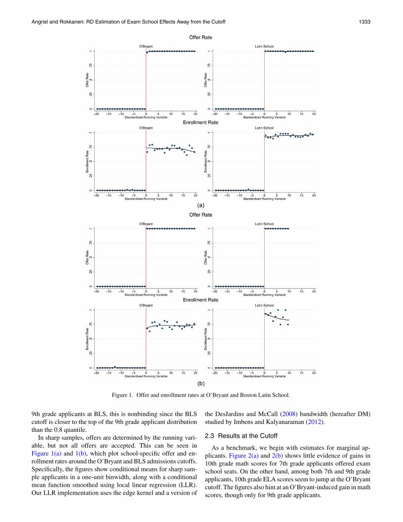
Figure 1. Offer and enrollment rates at O’Bryant and Boston Latin School.

9th grade applicants at BLS, this is nonbinding since the BLScutoff is closer to the top of the 9th grade applicant distributionthan the 0.8 quantile.

In sharp samples, offers are determined by the running vari-able, but not all offers are accepted. This can be seen inFigure 1(a) and 1(b), which plot school-specific offer and en-rollment rates around the O’Bryant and BLS admissions cutoffs.Specifically, the figures show conditional means for sharp sam-ple applicants in a one-unit binwidth, along with a conditionalmean function smoothed using local linear regression (LLR).Our LLR implementation uses the edge kernel and a version of

the DesJardins and McCall (2008) bandwidth (hereafter DM)studied by Imbens and Kalyanaraman (2012).

2.3 Results at the Cutoff

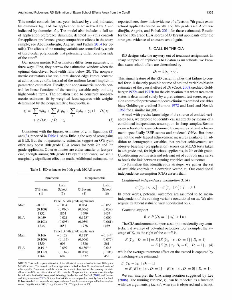
As a benchmark, we begin with estimates for marginal ap-plicants. Figure 2(a) and 2(b) shows little evidence of gains in10th grade math scores for 7th grade applicants offered examschool seats. On the other hand, among both 7th and 9th gradeapplicants, 10th grade ELA scores seem to jump at the O’Bryantcutoff. The figures also hint at an O’Bryant-induced gain in mathscores, though only for 9th grade applicants.

1334 Journal of the American Statistical Association, December 2015

Figure 2. 10th grade math and ELA scores at O’Bryant and Boston Latin School.

Our estimators of the effect of an exam school offer are de-rived from models for potential outcomes. Let Y1i and Y0i denotepotential outcomes in treated and untreated states, with the ob-served outcome determined by

yi = Y0i + (Y1i − Y0i)Di.

In a parametric setup, the conditional mean functions for poten-tial outcomes given the running variable are modeled as

E [Y0i | ri] = f0 (ri)

E [Y1i | ri] = ρ + f1 (ri) ,

using polynomials, fj (ri) ; j = 0, 1, that have the same inter-cept, so that conditional mean shifts are parameterized by ρ.

Substituting these polynomials in E [yi | ri] = (1−Di)E [Y0i | ri]+DiE [Y1i | ri], and allowing for the fact that theestimation sample pools data from different test years and appli-cation years, the equation used to construct parametric estimates,fit by ordinary least squares, is

yi =∑t

αthit +∑j

βjpij +∑�

δ�di� + (1−Di) f0 (ri)

+Dif1 (ri)+ ρDi + ηi. (2)

Angrist and Rokkanen: RD Estimation of Exam School Effects Away from the Cutoff 1335

This model controls for test year, indexed by t and indicatedby dummies hit , and for application year, indexed by � andindicated by dummies di�. The model also includes a full setof application preference dummies, denoted pij (this controlsfor applicant-preference-group composition effects in the sharpsample; see Abdulkadiroglu, Angrist, and Pathak 2014 for de-tails). The effects of the running variable are controlled by a pairof third-order polynomials that potentially differ on either sideof the cutoff.

Our nonparametric RD estimators differ from parametric inthree ways. First, they narrow the estimation window when theoptimal data-driven bandwidth falls below 20. The nonpara-metric estimators also use a tent-shaped edge kernel centeredat admissions cutoffs, instead of the uniform kernel implicit inparametric estimation. Finally, our nonparametric models con-trol for linear functions of the running variable only, omittinghigher-order terms. The equation used to construct nonpara-metric estimates, fit by weighted least squares with weightsdetermined by the nonparametric bandwidth, is

yi =∑t

αthit +∑j

βjpij +∑�

δ�di� + γ0 (1−Di) ri

+ γ1Diri + ρDi + ηi. (3)

Consistent with the figures, estimates of ρ in Equations (2)and (3), reported in Table 1, show little in the way of score gainsat BLS. But the nonparametric estimates suggest an O’Bryantoffer may boost 10th grade ELA scores for both 7th and 9thgrade applicants. Other estimates are either smaller or less pre-cise, though among 9th grade O’Bryant applicants, we see amarginally significant effect on math. Additional estimates, not

Table 1. RD estimates for 10th grade MCAS scores

Parametric Nonparametric

Latin LatinO’Bryant School O’Bryant School

(1) (3) (4) (6)

Panel A. 7th grade applicantsMath −0.011 −0.034 0.034 −0.055

(0.100) (0.060) (0.056) (0.039)1832 1854 1699 1467

ELA 0.059 0.021 0.125∗∗ 0.000(0.103) (0.095) (0.059) (0.061)1836 1857 1778 1459

Panel B. 9th grade applicantsMath 0.166 −0.128 0.128∗ −0.144∗

(0.109) (0.117) (0.066) (0.076)1559 606 1386 361

ELA 0.191∗ 0.097 0.180∗∗∗ 0.048(0.112) (0.187) (0.066) (0.106)1564 607 1532 458

NOTES: This table reports estimates of the effects of exam school offers on 10th gradeMCAS scores. The sample includes applicants ranked within 20 standardized units ofoffer cutoffs. Parametric models control for a cubic function of the running variable,allowed to differ on either side of offer cutoffs. Nonparametric estimates use the edgekernel, with bandwidth computed following DesJardins and McCall (2008) and Imbensand Kalyanaraman (2012). Optimal bandwidths were computed separately for each school.Robust standard errors are shown in parentheses. Sample sizes are reported below standarderrors. ∗significant at 10%; ∗∗significant at 5%; ∗∗∗significant at 1%.

reported here, show little evidence of effects on 7th grade examschool applicants tested in 7th and 8th grade (see Abdulka-diroglu, Angrist, and Pathak 2014 for these estimates). Resultsfor the 10th grade ELA scores of O’Bryant applicants offer thestrongest evidence of an exam school gain.

3. CALL IN THE CIA

RD designs take the mystery out of treatment assignment. Insharp samples of applicants to Boston exam schools, we knowthat exam school offers are determined by

Di = 1 [ri ≥ 0] .

This signal feature of the RD design implies that failure to con-trol for ri is the only possible source of omitted variables bias inestimates of the causal effect of Di (Cook 2008 credited Gold-berger 1972a and 1972b for the observation that when treatmentstatus is determined solely by a pretreatment test score, regres-sion control for pretreatment scores eliminates omitted variablesbias; Goldberger credited Barnow 1972 and Lord and Novick1968 for a similar insight).

Armed with precise knowledge of the source of omitted vari-ables bias, we propose to identify causal effects by means of aconditional independence assumption. In sharp samples, Bostonexam school offers are determined by measures of past achieve-ment, specifically ISEE scores and students’ GPAs. But theseare not the only lagged achievement measures available. In ad-dition to demographic variables that predict achievement, weobserve baseline (preapplication) scores on MCAS tests takenin 4th grade and, for high school applicants, in 7th or 8th grade.Conditioning on this rich and relevant set of controls may serveto break the link between running variables and outcomes.

To formalize this identification strategy, we gather the setof available controls in a covariate vector, xi. Our conditionalindependence assumption (CIA) asserts that:

Conditional independence assumption (CIA)

E[Yji | ri, xi

] = E [Yji | xi

]; j = 0, 1.

In other words, potential outcomes are assumed to be mean-independent of the running variable conditional on xi. We alsorequire treatment status to vary conditional on xi :

Common support

0 < P [Di = 1 | xi] < 1 a.s.

The CIA and common support assumptions identify any coun-terfactual average of potential outcomes. For example, the av-erage of Y0i to the right of the cutoff is

E [Y0i | Di = 1] = E {E [Y0i | xi,Di = 1] | Di = 1}= E {E [yi | xi,Di = 0] | Di = 1} , (4)

while the average treatment effect on the treated is captured bya matching-style estimand:

E [Y1i − Y0i | Di = 1]= E {E [yi | xi,Di = 1]− E [yi | xi,Di = 0] | Di = 1} .

We can interpret the CIA using notation suggested by Lee(2008). The running variable, ri , can be modeled as a functionwith two arguments g (xi, εi), where xi is observed and εi is not.

1336 Journal of the American Statistical Association, December 2015

Conditional on xi , the only source of variation in ri , and con-sequently in Di , is εi . Thus, the CIA requires that, conditionalon the observed xi , potential outcomes are mean-independentof unobserved determinants of the running variable.

3.1 Testing

Just as with conventional matching strategies for the iden-tification of treatment effects (as in, e.g., Heckman, Ichimura,and Todd 1998; Dehejia and Wahba 1999), the CIA assumptioninvoked here breaks the link between treatment status and po-tential outcomes, opening the door to identification of a widerange of average causal effects. In this case, however, the priorinformation inherent in an RD design is also available to guideour choice of the conditioning vector, xi . Specifically, under theCIA, we have

E [Y1i | ri, xi, ri ≥ 0] = E [Y1i | xi] = E [Y1i | xi, ri ≥ 0] ,

so we should expect that covariates that satisfy the CIA obey

E [yi | ri, xi,Di = 1] = E [yi | xi,Di = 1] , (5)

to the right of the cutoff. Likewise, the CIA implies

E [Y0i | ri, xi, ri < 0] = E [Y0i | xi] = E [Y0i | xi, ri < 0] ,

so we should expect that covariates that satisfy the CIA alsosatisfy

E [yi | ri, xi,Di = 0] = E [yi | xi,Di = 0] , (6)

to the left of the cutoff.Regressions of outcomes on xi and ri on either side of the

cutoff provide a simple test for restrictions (5) and (6). Meanindependence is stronger than regression independence, but re-gression testing procedures can embed flexible, nonlinear con-ditional mean functions. In practice, simple regression-basedtests seem preferable to more elaborate tests that may lack thepower to detect violations.

The CIA has a further testable implication: RD estimates andmatching-style estimates should differ only in how they weightcovariate-specific treatment effects. The CIA can therefore beevaluated by comparing RD estimates to properly reweighted(using the distribution of covariates at the cutoff) matching-styleestimates. The online supplementary materials explore this ideain detail.

3.2 Alternative Approaches

Battistin and Rettore (2008) consider matching estimates inan RD setting, focusing on fuzzy RD with one-sided noncompli-ance. They do not exploit an RD-specific conditional indepen-dence condition. Rather, in the spirit of Lalonde (1986), Battistinand Rettore validate a generic matching estimator for the aver-age treatment effect on the treated by comparing nonparametricRD estimates with conventional matching estimates constructedat the cutoff. They argue that when matching and RD producesimilar results at the cutoff, matching seems worth exploringaway from the cutoff as well. Mealli and Rampichini (2012)explored a similar approach, also using information away fromthe cutoff.

Other related discussions of RD identification away from thecutoff include DiNardo and Lee (2011) and Lee and Lemieux(2010), both of which note that the local interpretation of non-parametric RD estimates can be relaxed by treating the runningvariable as random rather than conditioning on it. In this view,observed running variable values are the realization of a nonde-generate stochastic process that assigns values to individuals ofan underlying type. Each type contributes to local-to-cutoff av-erage treatment effects in proportion to that type’s likelihood ofbeing represented at the cutoff. Since “type” is an inherently la-tent construct, this random running variable interpretation doesnot immediately offer concrete guidance as to how causal effectsmight change away from the cutoff. In the spirit of this notionof latent conditioning, however, we might model the runningvariables and conditioning variables in our CIA assumption asnoisy measures of a single underlying ability measure. Rokka-nen (2015) develops an RD framework in which identificationis based on this sort of latent factor ignorability. Finally, Dongand Lewbel (2012) considered identification of the effect ofchanging the threshold in an RD design.

3.3 CIA-Based Estimators

At specific running variable values, the CIA leads to the fol-lowing matching-style estimand:

E[Y1i − Y0i | ri = c]= E[E[yi | xi,Di = 1]− E[yi | xi,Di = 0] | ri = c]. (7)

Alternately, to the right of the cutoff, we might consider causaleffects averaged over all positive values up to c, a bounded effectof treatment on the treated:

E[Y1i − Y0i | 0 ≤ ri ≤ c] = E{E[yi | xi,Di = 1]

− E[yi | xi,Di = 0] | 0 ≤ ri ≤ c}. (8)

Paralleling this on the left, the bounded effect of treatment onthe nontreated is

E[Y1i − Y0i | −c ≤ ri < 0] = E{E[yi | xi,Di = 1]

− E[yi | xi,Di = 0] | −c ≤ ri < 0}. (9)

We estimate the parameters described by Equations (7)–(9) intwo ways. The first is a linear reweighting estimator discussed byKline (2011). The second is a version of the Hirano, Imbens, andRidder (2003) propensity score estimator based on Horvitz andThompson (1952). We also use the estimated propensity score todocument common support, as in Dehejia and Wahba’s (1999)pioneering propensity score study of the effect of a trainingprogram on earnings.

Kline’s reweighting estimator begins with linear models forconditional means, which can be written

E [yi | xi,Di = 0] = x ′iβ0 (10)

E [yi | xi,Di = 1] = x ′iβ1.

Linearity is not very restrictive since x ′iβj can include dummyvariables, polynomials, and interactions. Substituting in Equa-tion (7), we have

E [Y1i − Y0i | ri = c]= (β1 − β0)′ E [xi | ri = c] . (11)

Angrist and Rokkanen: RD Estimation of Exam School Effects Away from the Cutoff 1337

Linear reweighting estimators are given by the sample analogof (11) and analogous expressions based on Equations (8) and(9).

Letting λ (xi) ≡ E [Di | xi] denote the propensity score,our propensity score weighting estimator begins with theobservation that the CIA implies

E

[yi (1−Di)

1− λ (xi)| xi

]= E [Y0i | xi]

E

[yiDi

λ (xi)| xi

]= E [Y1i | xi] .

Bringing these expressions inside a single expectation and overa common denominator, the treatment effect on the treated forthose with 0 ≤ ri ≤ c is given by

E [Y1i − Y0i | 0 ≤ ri ≤ c]= E

{yi [Di − λ (xi)]

λ (xi) [1− λ (xi)]× P [0 ≤ ri ≤ c | xi]

P [0 ≤ ri ≤ c]}. (12)

Propensity score weighting estimators are given by the sampleanalog of Equation (12) and similar formulas for the averageeffect on nontreated applicants and average effects at specific,possibly narrow, ranges of running variable values.

The empirical counterpart of Equation (12) requires a modelfor the probability P [0 ≤ ri ≤ c | xi] as well as for λ (xi). Itseems natural to use the same parameterization for both. Notealso that if c equals the upper bound of the support of ri , theestimand in Equation (12) simplifies to

E [Y1i − Y0i | Di = 1] = E{yi [Di − λ (xi)]

[1− λ (xi)]E [Di]

},

as in Hirano, Imbens, and Ridder (2003).When the estimand targets average effects at specific running

variable values, say ri = c, as opposed to over an interval, theprobabilities that appear in Equation (12) become densities.Note also that the estimand in Equation (12) can be written asE [ω1iyi − ω0iyi], for weights, ω1i and ω0i such that E [ω0i] =E [ω1i] = 1. As noted by Imbens (2004), this normalizationneed not hold in finite samples. We therefore normalize the sumof our empirical weights to be 1.

4. THE CIA IN ACTION AT BOSTON EXAM SCHOOLS

We start by testing CIA in estimation windows of±20 aroundthe O’Bryant and BLS cutoffs. Limiting attention to these win-dows mitigates bias from changing counterfactuals as distancefrom the cutoff grows. Moving, say, to the left of the BLS cut-off, BLS applicants start to fall below the BLA cutoff as well,thereby changing the relevant counterfactual school from BLAto O’Bryant for BLS applicants not offered a seat there. Theresulting change in Y0i (where potential outcomes are indexedagainst BLS offers) is likely to be correlated with the BLS run-ning variable with or without conditioning on xi .

To see how this correlation arises, note that when estimatinga BLS treatment effect, outcomes at BLS determine the relevantY1i , while those at other schools determine Y0i . Just to the left ofthe BLS cutoff, most applicants enroll at BLA, generating Y BLA

0i .Further to the left, however, below a cutoff, b, BLS applicantsno longer qualify for BLA, and therefore end up at O’Bryant.The outcome observed for this group is YOBR

0i . For those in the

Table 2. Conditional independence tests

O’Bryant Latin School

D = 0 D = 1 D = 0 D = 1(1) (2) (3) (4)

Panel A. 7th grade applicantsMath 0.022∗∗∗ 0.015∗∗∗ 0.008∗∗∗ 0.014∗∗∗

(0.004) (0.004) (0.002) (0.002)838 618 706 748

ELA 0.015∗∗∗ 0.006 0.013∗∗∗ 0.018∗∗∗

(0.004) (0.005) (0.003) (0.003)840 621 709 750

Panel B. 9th grade applicantsMath 0.002 0.005 0.008∗∗ 0.018

(0.004) (0.003) (0.003) (0.028)513 486 320 49

ELA 0.003 0.002 0.006 0.055(0.004) (0.004) (0.005) (0.053)

516 489 320 50

NOTES: This table reports regression-based tests of the conditional independence assump-tion described in the text. Cell entries show the coefficient on the same-subject runningvariable in models for 10th grade math and ELA scores that control for baseline scores,along with indicators for special education status, limited English proficiency, eligibility forfree or reduced price lunch, race (black/Asian/Hispanic), and sex. Estimates use only ob-servations to the left or right of the cutoff as indicated in column headings. Robust standarderrors are reported in parentheses. Sample sizes are reported below standard errors (samplesare limited to applicants within 20 points of the cutoff). ∗significant at 10%; ∗∗significantat 5%; ∗∗∗significant at 1%.

BLS applicant pool, we can therefore write

Y0i = Y BLA0i +

(YOBR

0i − Y BLA0i

)1 [ri < b] .

Under the CIA, conditioning on xi eliminates the dependence ofpotential outcomes Y BLA

0i and YOBR0i on ri . But the switch from

Y BLA0i to YOBR

0i at b remains, inducing dependence between Y0i

and ri unless the distinction between BLA and O’Bryant is of noconsequence. We therefore insure against bias from changingcounterfactuals by limiting extrapolation to the left of the BLScutoff when looking at BLS applicants.

The regressions used to test the CIA include controls for base-line test scores along with indicators of special education status,limited English proficiency, eligibility for free or reduced pricelunch, race (black/Asian/Hispanic), and sex, as well as indica-tors for test year, application year, and application preferences.Baseline score controls for 7th grade applicants consist of 4thgrade math and ELA scores, while for 9th grade applicants,baseline score controls add 7th grade ELA scores and 8th grademath scores.

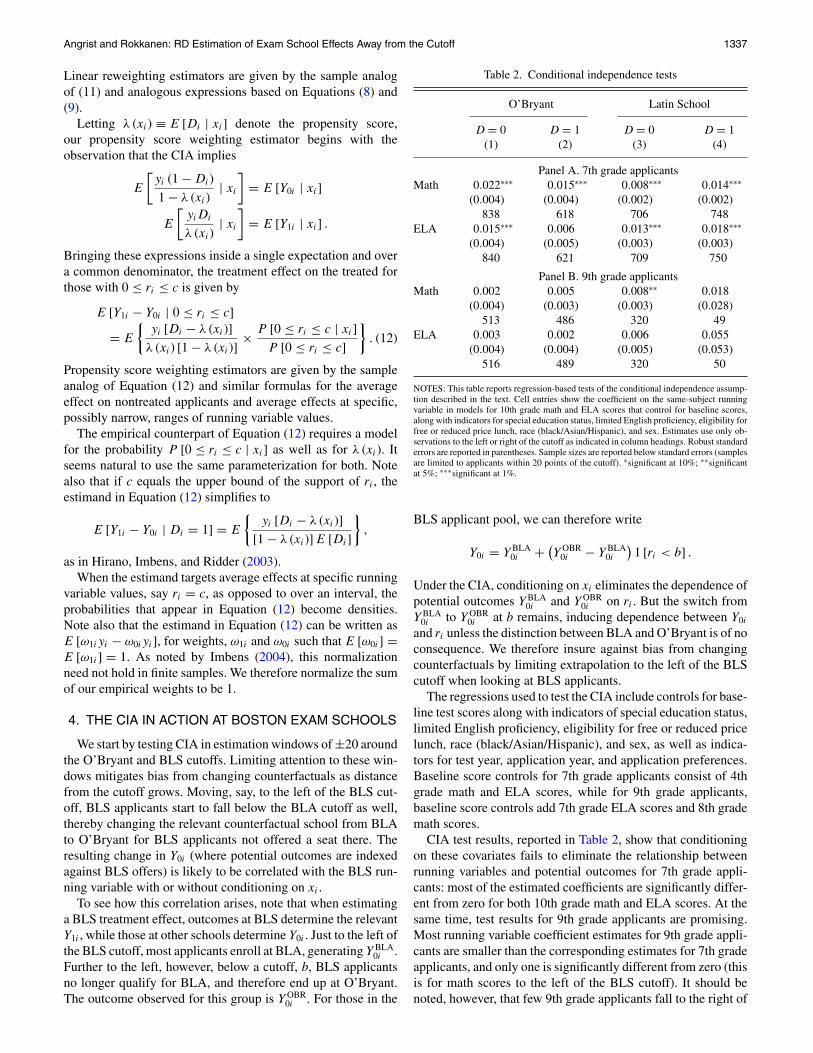
CIA test results, reported in Table 2, show that conditioningon these covariates fails to eliminate the relationship betweenrunning variables and potential outcomes for 7th grade appli-cants: most of the estimated coefficients are significantly differ-ent from zero for both 10th grade math and ELA scores. At thesame time, test results for 9th grade applicants are promising.Most running variable coefficient estimates for 9th grade appli-cants are smaller than the corresponding estimates for 7th gradeapplicants, and only one is significantly different from zero (thisis for math scores to the left of the BLS cutoff). It should benoted, however, that few 9th grade applicants fall to the right of

1338 Journal of the American Statistical Association, December 2015

Figure 3. Visual evaluation of the CIA in the window [−20,20] around exam school offer cutoffs.

the BLS cutoff. CIA tests for BLS applicants with Di = 1 areforgiving in part because the sample for this group is small.

We complement formal CIA testing with a graphical toolmotivated by an observation in Lee and Lemieux (2010): in arandomized trial using a uniformly distributed random numberto determine treatment assignment, the randomizer becomesthe running variable for an RD design. The relationship be-tween outcomes and this running variable should be flat, ex-cept possibly for a jump at the quantile cutoff that determines

treatment assignment. Our CIA assumption implies this samepattern for nonrandomized studies. Figure 3 therefore plots 10thgrade math and ELA residuals from regressions of the outcomeson xi against running variables. The figure shows conditionalmeans for all applicants in one-unit binwidths, along with con-ditional mean functions smoothed using local linear regression.Consistent with the test results reported in Table 2, Figure 3shows a strong positive relationship between outcome residualsand running variables for 7th grade applicants. For 9th grade

Angrist and Rokkanen: RD Estimation of Exam School Effects Away from the Cutoff 1339

Table 3. CIA estimates of the effect of exam school offers for 9thgrade applicants

Math ELA

Latin LatinO’Bryant School O’Bryant School

(1) (2) (3) (4)

Linear reweighting 0.156∗∗∗ −0.031 0.198∗∗∗ 0.088(0.039) (0.094) (0.041) (0.084)

N untreated 513 320 516 320N treated 486 49 489 50Propensity score weighting 0.131∗∗∗ −0.037 0.236∗∗∗ 0.031

(0.051) (0.057) (0.077) (0.109)N untreated 509 320 512 320N treated 482 49 485 50

NOTES: This table reports CIA estimates of the effect of exam school offers on MCASscores for 9th grade applicants to O’Bryant and BLS. The first row reports results from alinear reweighting estimator, and the second row reports results from inverse propensityscore weighting, as described in the text. Controls are the same as used to construct thetest statistics reported in Table 2 except that the propensity score models for Latin Schoolomit test year and application preference dummies. The O’Bryant estimates are effects onnontreated applicants to the left of the admissions cutoff; the BLS estimates are effects ontreated applicants to the right of the cutoff. Standard errors (shown in parentheses) werecomputed using a nonparametric bootstrap with 500 replications. The number of treatedand untreated (offered and not offered) observations in the relevant outcome samples appearbelow standard errors. ∗significant at 10%; ∗∗significant at 5%; ∗∗∗significant at 1%.

applicants, however, the relationship between outcome residu-als and running variables is essentially flat, except perhaps forELA scores in the BLS sample.

In combination with demographic control variables and 4thgrade scores, 7th and 8th grade MCAS scores appear to do agood job of removing dependence on the running variable in 9thgraders’ conditional mean functions for 10th grade scores. Thedifference in CIA test results for 7th and 9th grade applicantsmay reflect the fact that baseline scores for 9th grade applicants

come from tests taken in a grade closer to the outcome test gradethan baseline scores for 7th grade applicants (the most recentbaseline test scores available for 7th grade applicants are from4th grade tests). In view of the results in Table 2 and Figure 3,the CIA-based estimates that follow are for 9th grade applicantsonly.

The first row of Table 3 reports linear reweighting estimatesof average treatment effects computed using covariate speci-fications that parallel those used for the CIA tests. These areestimates ofE [Y1i − Y0i | 0 ≤ ri ≤ 20] for BLS applicants andE [Y1i − Y0i | −20 ≤ ri < 0] for O’Bryant applicants. Specifi-cally, the estimand for BLS is

E [Y1i − Y0i | 0 ≤ ri ≤ 20]= (β1 − β0)′ E [xi | 0 ≤ ri ≤ 20] , (13)

while that for O’Bryant is

E [Y1i − Y0i | −20 ≤ ri < 0]= (β1 − β0)′ E [xi | −20 ≤ ri < 0] , (14)

where β0 and β1 are defined in Equation (10). The BLS es-timand is an average effect of treatment on the treated, whilethe O’Bryant estimand is an average effect of treatment on thenontreated.

As with RD estimates at the cutoff, the CIA-based estimatesin Table 3 show no evidence of a BLS achievement boost. Atthe same time, results for inframarginal unqualified O’Bryantapplicants offer some evidence of gains. The estimates for mathand ELA are on the order of 0.16σ and 0.2σ , both significantlydifferent from zero. These CIA estimates are remarkably con-sistent with the corresponding RD estimates at the cutoff.

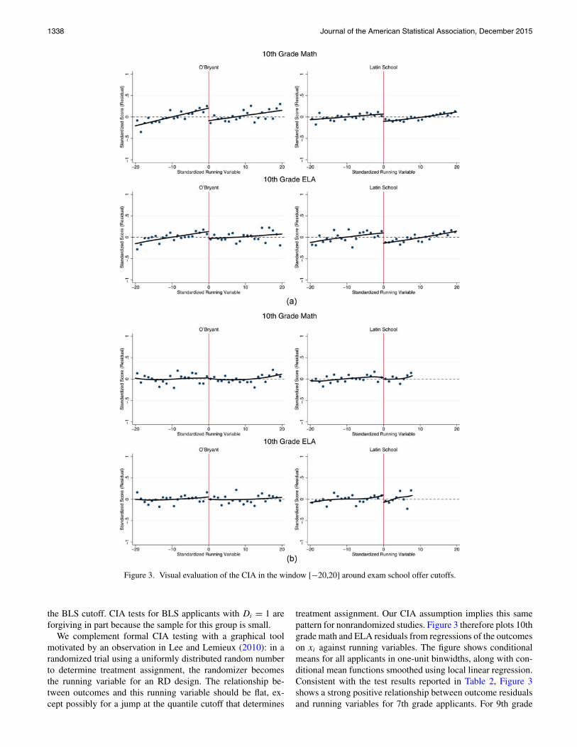
Figure 4 completes the picture of effects away from the cutoffby plotting linear reweighting estimates of E [Y1i | ri = c] andE [Y0i | ri = c] for all values of c in the [−20, 20] interval. To

Figure 4. CIA-based estimates of E [Y1i | ri = c] and E [Y0i | ri = c] for c in the window[−20, 20] for 9th grade applicants.

1340 Journal of the American Statistical Association, December 2015

Figure 5. Histograms of estimated propensity scores in the window[−20, 20] for 9th grade applicants to O’Bryant and BLS.

the left of the O’Bryant cutoff, the estimates of E [Y0i | ri = c]are fitted values from regression models for observed outcomes,while the estimates ofE [Y1i | ri = c] are an extrapolation basedon Equation (10). To the right of the BLS cutoff, the esti-mates of E [Y1i | ri = c] are fitted values while the estimatesof E [Y0i | ri = c] are an extrapolation based on Equation (10).The conditional means in this figure were constructed by plug-ging individual values of xi into Equation (10) and smoothingthe results using local linear regression (using the edge kernelwith Stata’s default bandwidth). The figure presents a pictureconsistent with that suggested by the estimates in Table 3. Inparticular, the extrapolated BLS effects are small (for ELA) ornoisy (for math), while the O’Bryant extrapolation reveals a re-markably stable gain in ELA scores away from the cutoff. Theextrapolated effect of O’Bryant offers on math scores appearsto increase modestly as a function of distance from the cutoff, afinding probed further below.

4.1 Propensity Score Estimates

CIA-based estimation of the effect of exam school offersseems like a good setting for estimation using propensity scoremethods, since the conditioning set in this case includes multiplecontinuously distributed control variables. This set of controlscomplicates full covariate matching. Our logit model for thepropensity score incorporates the control variables and param-eterization used to construct the tests in Table 2 and the linearreweighting estimates in the first row of Table 3 (the logit modelfor the smaller sample of BLS applicants omits test year andapplication preference dummies).

The estimated propensity score distributions for admitted andrejected applicants exhibit a substantial degree of overlap. Thisis documented in Figure 5, which plots the histogram of propen-sity score fitted values for treated and control observations aboveand below a common horizontal axis. Not surprisingly, the larger

sample of O’Bryant applicants generates more overlap than therelatively narrow sample for highly selective BLS. Most scorevalues for untreated O’Bryant applicants fall below about 0.6.But each decile in the O’Bryant score distribution contains atleast a few treated observations; above the first decile, there ap-pear to be more than enough for accurate inference. By contrast,few untreated BLS applicants have covariate values for whicha BLS offer is highly likely. We should therefore expect BLScounterfactual averages to be estimated less precisely than thosefor O’Bryant.

The propensity-score-weighted estimates reported in the bot-tom half of Table 3 are consistent with the linear reweightingestimates shown in the first row of the table. In particular, theestimates here suggest most BLS students would do no worse ifthey had to go to BLA instead, while low scoring O’Bryant ap-plicants might enjoy substantial gains in ELA where they offereda seat at O’Bryant. It also seems noteworthy that most of thepropensity score estimates are somewhat less precise than thecorresponding linear reweighting estimates. Linear reweightinglooks like an attractive procedure in this context.

5. FUZZY CIA MODELS

Exam school offers affect achievement by facilitating examschool enrollment. The magnitude of offer comparisons—implicitly a reduced form for instrumental variables (IV) mod-els with endogenous enrollment—is therefore easier to interpretwhen the relevant enrollment first-stage estimates scale theseeffects. Use of sharply determined exam school offers to in-strument a mediating causal variable like enrollment leads to afuzzy RD design. If the fuzzy-RD enrollment first stage changesas a function of the running variable, comparisons of reducedform estimates across running variable values are meaningfulonly after rescaling. In principle, IV estimators like two-stage

Angrist and Rokkanen: RD Estimation of Exam School Effects Away from the Cutoff 1341

least squares (2SLS) make the appropriate adjustment. A ques-tion that arises here, however, is how to interpret IV estimatesconstructed under the CIA in a world of heterogenous poten-tial outcomes, where the average causal effects identified by IVpotentially vary with the running variable.

We estimate and interpret the causal effects of exam schoolenrollment by adapting the local average treatment effectsframework outlined by Imbens and Angrist (1994) and extendedby Abadie (2003). This framework allows for unrestricted treat-ment effect heterogeneity in potentially nonlinear IV modelswith covariates. The starting point is notation for potential treat-ment assignments,W0i andW1i , indexed against the instrument,in this case, exam school offers indicated by Di. Thus, W0i

indicates (eventual) exam school enrollment among those notoffered a seat, while W1i indicates (eventual) exam school en-rollment among those offered a seat. Observed enrollment statusis

Wi = W0i (1−Di)+W1iDi.

The core identifying assumption in our IV setup, together withthe common support assumption given in Section 3, is a gener-alized version of CIA:

Generalized conditional independence assumption (GCIA)

(Y0i , Y1i ,W0i ,W1i) ⊥⊥ ri | xi.The GCIA generalizes simple CIA in three ways. First, GCIAimposes full independence instead of mean independence; thisseems innocuous since any treatment assignment mechanismsatisfying the latter is likely to satisfy the former. Second, alongwith potential outcomes, the pair of potential treatment assign-ments (W0i andW1i) is taken to be conditionally independent ofthe running variable. Finally, GCIA requires joint independenceof all potential outcome and assignment variables, while theCIA in Section 3 requires only marginal (mean) independence.Again, it is hard to see why we would have the latter withoutthe former.

5.1 Fuzzy Identification

5.1.1 Local Average Treatment Effects. In the local averagetreatment effects (LATE) framework, the subset of compliersconsists of people whose treatment status can be changed bychanging a Bernoulli instrument. This group is defined here byW1i > W0i . In addition to the GCIA, a key identifying assump-tion in the LATE framework is monotonicity: the instrumentshifts treatment only one way. Assuming that the instrumentDi

satisfies monotonicity with W1i ≥ W0i , and that for some i theinequality is strict, so there is a first stage, the LATE theorem(Imbens and Angrist 1994) tells us that

E [yi | Di = 1]− E [yi | Di = 0]

E [Wi | Di = 1]− E [Wi | Di = 0]

= E [Y1i − Y0i | W1i > W0i] .

In other words, a Wald-type IV estimand given by the ratio ofreduced-form offer effects to first-stage offer effects capturesaverage causal effects on exam school applicants who enrollwhen they receive an offer but not otherwise.

Abadie (2003) generalized the LATE theorem by showingthat the expectation of any measurable function of treatment,

covariates, and outcomes is identified for compliers. This resultfacilitates IV estimation using a wide range of causal models,including nonlinear models such as those based on the propen-sity score. Here, we adapt the Abadie (2003) result to a fuzzyRD setup that identifies causal effects away from the cutoff.This requires a conditional first stage, described below:

Conditional first stage

P [W1i = 1 | xi] > P [W0i = 1 | xi] a.s.

Given GCIA, common support, monotonicity, and a condi-tional first stage, the following identification result can be es-tablished (see the online appendix for proof):

Theorem 1 (Fuzzy CIA Effects)

E [Y1i − Y0i | W1i > W0i , 0 ≤ ri ≤ c]

= 1

P [W1i > W0i | 0 ≤ ri ≤ c]

×E{ψ (Di, xi)

P [0 ≤ ri ≤ c | xi]P [0 ≤ ri ≤ c] yi

}, (15)

where ψ (Di, xi) ≡ Di − λ (xi)

λ (xi) [1− λ (xi)].

Estimators based on Equation (15) capture causal effects forcompliers with running variable values falling into any rangeover which there is common support.

At first blush, it is not immediately clear howto estimate the conditional compliance probability,P [W1i > W0i | 0 ≤ ri ≤ c], appearing in the denomina-tor of Equation (15). Because everyone to the right of the cutoffis offered treatment, there would seem to be no data availableto estimate compliance rates conditional on 0 ≤ ri ≤ c (in theLATE framework, the IV first stage measures the probabilityof compliance). Paralleling an argument in Abadie (2003),however, the online appendix shows that

P [W1i > W0i | 0 ≤ ri ≤ c]= E

{κ (Wi,Di, xi)

P [0 ≤ ri ≤ c | xi]P [0 ≤ ri ≤ c]

}, (16)

where

κ (Wi,Di, xi) ≡ 1− Wi (1−Di)

1− λ (xi)− (1−Wi)Di

λ (xi).

The online appendix provides further details for this fuzzy esti-mation strategy and describes an alternative implementation ofTheorem 1 that offers a computational simplification (estimatesusing the alternative approach are similar to those reported here).

5.1.2 Average Causal Response. The causal frameworkleading to Theorem 1 is limited to Bernoulli endogenous vari-ables. For some applicants, however, the exam school treatmentis mediated by years of attendance rather than a simple go/no-godecision. We develop a fuzzy CIA estimator for such orderedtreatments by adapting a result from Angrist and Imbens (1995).This extension relies on potential outcomes indexed against anordered treatment, wi . Specifically, let Yji denote the poten-tial outcome when wi = j , for j = 0, 1, 2, . . . , J . We assume

1342 Journal of the American Statistical Association, December 2015

also that potential treatments,w1i andw0i , satisfy monotonicitywith w1i ≥ w0i , and that these potential treatments generate aconditional first stage. In other words,

E [w1i | xi] �= E [w0i | xi]for the same conditioning variables that give us a valid GCIA.

The Angrist and Imbens (1995) average causal response(ACR) theorem is a key building block in our analysis of or-dered treatment effects identified using the GCIA. This theoremdescribes the Wald IV estimand as follows:

E [yi | Di = 1]− E [yi | Di = 0]

E [wi | Di = 1]− E [wi | Di = 0]

=∑j

νjE[Yji − Yj−1,i | w1i ≥ j > w0i

],

where νj = P [w1i ≥ j > w0i]∑� P [w1i ≥ � > w0i]

= P [wi ≤ j | Di = 0]− P [wi ≤ j | Di = 1]

E [wi | Di = 1]− E [wi | Di = 0].

Wald-type IV estimators capture a weighted average of the aver-age causal effect of increasing wi from j − 1 to j, for complierswhose treatment intensity is moved by the instrument from be-low j to above j. The weights are given by the impact of theinstrument on the cumulative distribution function (CDF) of theendogenous variable at each level of treatment intensity.

The GCIA assumption allows us to establish a similar resultin a fuzzy RD setup with an ordered treatment. The followingis shown in our online appendix:

Theorem 2 (Fuzzy Average Causal Response)

E {E [yi | Di = 1, xi]− E [yi | Di = 0, xi] | 0 ≤ ri ≤ c}E {E [wi | Di = 1, xi]− E [wi | Di = 0, xi] | 0 ≤ ri ≤ c}=

∑j

νjcE[Yji − Yj−1,i | w1i ≥ j > w0i , 0 ≤ ri ≤ c

],

(17)

where

νjc = P [w1i ≥ j > w0i | 0 ≤ ri ≤ c]∑� P [w1i ≥ � > w0i | 0 ≤ ri ≤ c] . (18)

This theorem says that a Wald-type estimator constructed byaveraging covariate-specific first stages and reduced forms cap-tures a weighted average causal response for compliers withrunning variable values in the desired range. The incrementalaverage causal response, E[Yji − Yj−1,i | w1i ≥ j > w0i , 0 ≤ri ≤ c], is weighted by the conditional (on 0 ≤ ri ≤ c) proba-bility that the instrument moves the ordered treatment throughthe point at which the incremental effect is evaluated.

In practice, we estimate the left-hand side of Equation (17)by fitting linear models that include covariate interactions to thereduced form and first stage. The resulting estimation proce-dure adapts Kline (2011) to an ordered treatment and works asfollows: estimate conditional linear reduced forms interactingDi and xi ; use these estimates to construct the desired averagereduced form effect as in Equations (13) and (14); divide by asimilarly constructed average first stage. The same procedurecan be used to estimate Equation (17) for a Bernoulli treatment

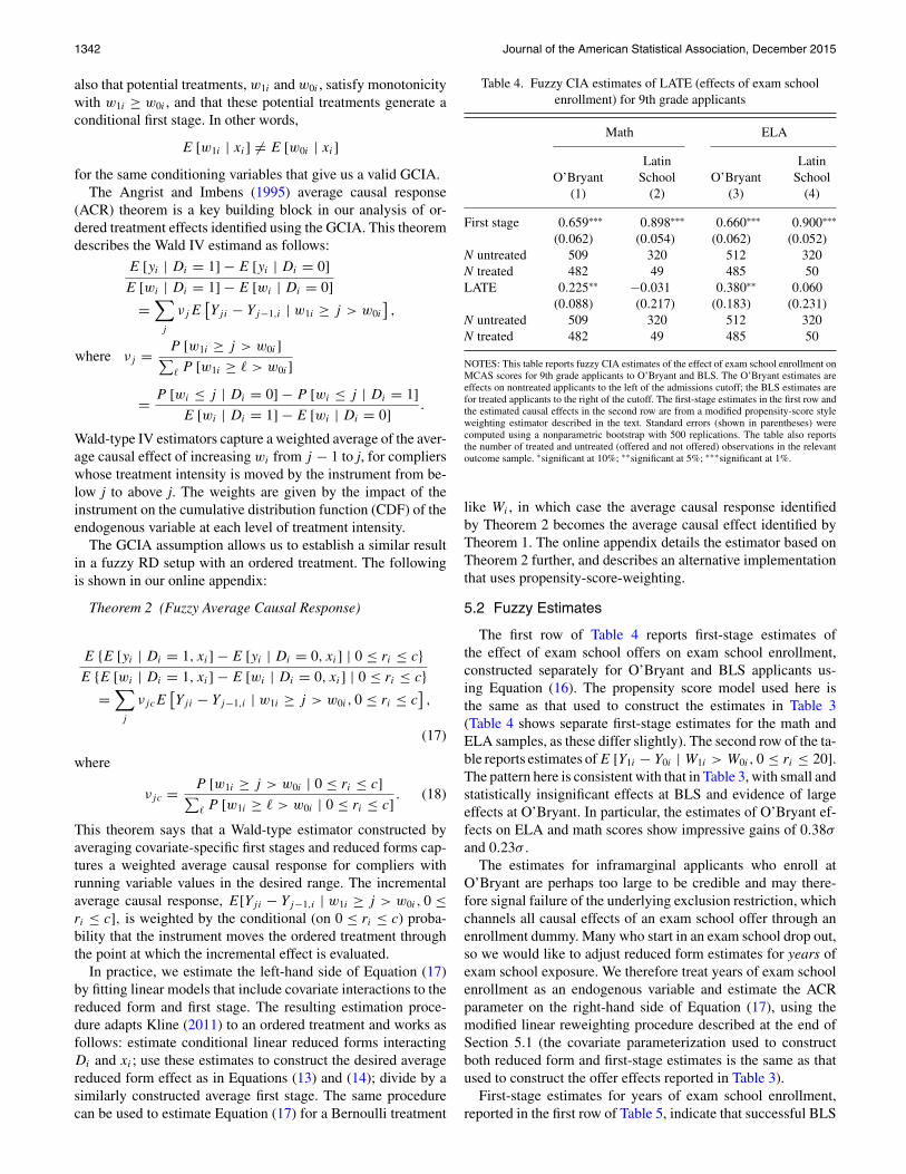
Table 4. Fuzzy CIA estimates of LATE (effects of exam schoolenrollment) for 9th grade applicants

Math ELA

Latin LatinO’Bryant School O’Bryant School

(1) (2) (3) (4)

First stage 0.659∗∗∗ 0.898∗∗∗ 0.660∗∗∗ 0.900∗∗∗

(0.062) (0.054) (0.062) (0.052)N untreated 509 320 512 320N treated 482 49 485 50LATE 0.225∗∗ −0.031 0.380∗∗ 0.060

(0.088) (0.217) (0.183) (0.231)N untreated 509 320 512 320N treated 482 49 485 50

NOTES: This table reports fuzzy CIA estimates of the effect of exam school enrollment onMCAS scores for 9th grade applicants to O’Bryant and BLS. The O’Bryant estimates areeffects on nontreated applicants to the left of the admissions cutoff; the BLS estimates arefor treated applicants to the right of the cutoff. The first-stage estimates in the first row andthe estimated causal effects in the second row are from a modified propensity-score styleweighting estimator described in the text. Standard errors (shown in parentheses) werecomputed using a nonparametric bootstrap with 500 replications. The table also reportsthe number of treated and untreated (offered and not offered) observations in the relevantoutcome sample. ∗significant at 10%; ∗∗significant at 5%; ∗∗∗significant at 1%.

like Wi , in which case the average causal response identifiedby Theorem 2 becomes the average causal effect identified byTheorem 1. The online appendix details the estimator based onTheorem 2 further, and describes an alternative implementationthat uses propensity-score-weighting.

5.2 Fuzzy Estimates

The first row of Table 4 reports first-stage estimates ofthe effect of exam school offers on exam school enrollment,constructed separately for O’Bryant and BLS applicants us-ing Equation (16). The propensity score model used here isthe same as that used to construct the estimates in Table 3(Table 4 shows separate first-stage estimates for the math andELA samples, as these differ slightly). The second row of the ta-ble reports estimates ofE [Y1i − Y0i | W1i > W0i , 0 ≤ ri ≤ 20].The pattern here is consistent with that in Table 3, with small andstatistically insignificant effects at BLS and evidence of largeeffects at O’Bryant. In particular, the estimates of O’Bryant ef-fects on ELA and math scores show impressive gains of 0.38σand 0.23σ .

The estimates for inframarginal applicants who enroll atO’Bryant are perhaps too large to be credible and may there-fore signal failure of the underlying exclusion restriction, whichchannels all causal effects of an exam school offer through anenrollment dummy. Many who start in an exam school drop out,so we would like to adjust reduced form estimates for years ofexam school exposure. We therefore treat years of exam schoolenrollment as an endogenous variable and estimate the ACRparameter on the right-hand side of Equation (17), using themodified linear reweighting procedure described at the end ofSection 5.1 (the covariate parameterization used to constructboth reduced form and first-stage estimates is the same as thatused to construct the offer effects reported in Table 3).

First-stage estimates for years of exam school enrollment,reported in the first row of Table 5, indicate that successful BLS

Angrist and Rokkanen: RD Estimation of Exam School Effects Away from the Cutoff 1343

Table 5. Fuzzy CIA estimates of average causal response (effect ofyears of enrollment) for 9th grade applicants

Math ELA

Latin LatinO’Bryant School O’Bryant School

(1) (2) (3) (4)

First stage 1.394∗∗∗ 1.816∗∗∗ 1.398∗∗∗ 1.820∗∗∗

(0.064) (0.096) (0.065) (0.093)N untreated 513 320 516 320N treated 486 49 489 50ACR 0.112∗∗∗ −0.017 0.142∗∗∗ 0.048

(0.029) (0.050) (0.030) (0.045)N untreated 513 320 516 320N treated 486 49 489 50

NOTES: This table reports fuzzy RD estimates of the effect of years of exam schoolenrollment on MCAS scores for 9th grade applicants to O’Bryant and BLS. The O’Bryantestimates are effects on nontreated applicants to the left of the admissions cutoff; the BLSestimates are for treated applicants to the right of the cutoff. The first-stage estimates in thefirst row and the estimated causal effects in the second row are from a modified linear 2SLSestimator described in the text. Standard errors (shown in parentheses) were computedusing a nonparametric bootstrap with 500 replications. The table also reports the number oftreated and untreated (offered and not offered) observations in the relevant outcome sample.∗significant at 10%; ∗∗significant at 5%; ∗∗∗significant at 1%.

applicants spent about 1.8 years at BLS between their examschool application and (outcome) test date, while successfulO’Bryant applicants spent about 1.4 years at O’Bryant betweenapplication and test date. The associated ACR estimates, re-ported in the bottom half of Table 5, are in line with the LATEestimates in Table 4, but considerably more precise. For ex-ample, the effect of a year of BLS exposure on ELA scores isestimated to be no more than about 0.05σ , with a standard errorof roughly the same magnitude. This compares with an estimateof about the same size in column 4 of Table 4, but the standarderror for the latter is five times larger. The precision gain herewould seem to come from linearity of the estimator and notfrom the change in endogenous variable, since the underlyingreduced form relationship (which ultimately determines the pre-cision of any IV estimate) is the same for the LATE and ACRmodels. The results for O’Bryant show precisely estimated gainsof about 0.14σ and 0.11σ per year of exam school exposure.

6. SUMMARY AND DIRECTIONS FORFURTHER WORK

The causality-revealing power of RD comes in part from thefact that the only source of omitted variables bias in an RDdesign is the running variable. Our conditional independenceassumption therefore makes the running variable ignorable, thatis, independent of potential outcomes, by conditioning on otherpredictors of outcomes. When the running variable is ignor-able, treatment is ignorable. Although our CIA framework isdemanding and will not be appropriate for all RD applications,the conditional independence assumption at the heart of our ap-proach has testable implications that are easily checked. Specif-ically, the CIA implies that in samples limited to either treatedor control observations, regressions of outcomes on the runningvariable and the covariates that support CIA should show norunning variable effects.

Among 9th grade applicants to the O’Bryant school and BLS,the CIA appears to hold. Importantly, the conditioning variablessupporting this result include 7th or 8th grade and 4th gradeMCAS scores, all lagged versions of the 10th grade outcomevariable. Lagged middle school scores in particular seem likea key control, probably because these relatively recent baselinetests are a powerful predictor of future scores. Lagged outcomesare better predictors, in fact, than the running variable itself,which is a composite constructed from applicants’ GPAs and adistinct exam school admissions test.

Results based on the CIA suggest that inframarginal high-scoring BLS applicants gain little (in terms of achievement)from BLS attendance, a result consistent with the RD estimatesof BLS effects at the cutoff reported in Abdulkadiroglu, Angrist,and Pathak (2014). At the same time, CIA-based estimates usingboth linear and propensity score weighting models generate ro-bust evidence of gains in English for unqualified inframarginalO’Bryant applicants. Evidence of 10th grade ELA gains alsoemerge from the RD estimates of exam school effects reportedby Abdulkadiroglu, Angrist, and Pathak (2014), especially fornonwhites. The CIA-based estimates reported here suggest sim-ilar gains would likely be observed should the O’Bryant cutoffbe reduced to accommodate currently unqualified high schoolapplicants, perhaps as a result of reintroducing affirmative actionconsiderations in exam school admissions.

We also modify CIA-based identification strategies for fuzzyRD and use this modification to estimate the effects of examschool enrollment and years of exam school attendance, in ad-dition to the reduced form effects of exam school admissionsoffers. A fuzzy analysis allows us to explore the possibility thatvariation in reduced form offer effects as a function of the run-ning variable are driven by changes in an underlying first stagefor exam school exposure.

Our CIA-based extrapolation strategy is likely to prove usefulin many RD settings. For example, we have seen our frameworkapplied in recent and ongoing studies of merit scholarships andcollege enrollment (Bruce and Carruthers 2014), incumbencyadvantage in elections (Hainmueller, Hall, and Snyder 2014),employment protection and job security (Hijzen, Mondauto,and Scarpetta 2013), publicity requirements in public procure-ment (Coviello and Mariniello 2014), public guarantee schemesto small and medium enterprise borrowing (de Blasio, De Mitri,Alessio D’Ignazio, and Stoppani 2014), and public school fund-ing (Kreisman 2013). Our fuzzy extension also opens the doorto identification of causal effects for compliers in RD modelsfor quantile treatment effects. As noted recently by Frandsen,Frolich, and Melly (2012), the weighting approach used byAbadie, Angrist, and Imbens (2002) and Abadie (2003) breaksdown in a conventional RD framework because the distribu-tion of treatment status is degenerate conditional on the runningvariable. By taking the running variable out of the equation,our framework circumvents this problem, a feature we plan toexploit in future research on distributional outcomes. Finally, inrecent work, Rokkanen (2015) developed identification strate-gies for RD designs in which the CIA conditioning variable isan unobserved latent factor. Multiple noisy indicators of the un-derlying latent factor provide the key to away-from-the-cutoffidentification in this new context.

1344 Journal of the American Statistical Association, December 2015

SUPPLEMENTARY MATERIALS

The supplementary materials contain proofs and additionaltheoretical results, along with additional statistical tests andestimates of exam school effects away from the cutoff.

[Received December 2013. Revised January 2015.]

REFERENCES

Abadie, A. (2003), “Semiparametric Instrumental Variables Estimationof Treatment Response Models,” Journal of Econometrics, 113,231–263. [1341,1343]

Abadie, A., Angrist, J. D., and Imbens, G. (2002), “Instrumental VariablesEstimates of the Effect of Subsidized Training on the Quantiles of TraineeEarnings,” Econometrica, 70, 91–117. [1343]

Abdulkadiroglu, A., Angrist, J. D., and Pathak, P. (2014), “The Elite Illusion:Achievement Effects at Boston and New York Exam Schools,” Economet-rica, 82, 137–196. [1331,1332,1335,1335,1343]

Angrist, J. D., and Imbens, G. W. (1995), “Two-Stage Least Squares Es-timation of Average Causal Effects in Models with Variable TreatmentIntensity,” Journal of the American Statistical Association, 90, 431–442.[1341,1342]

Barnow, B. S. (1972), “Conditions for the Presence or Absence of a Biasin Treatment Effect: Some Statistical Models for Head Start Evaluation,”Discussion Paper 122-72, University of Wisconsin-Madison, Madison, WI.[1335]

Battistin, E., and Rettore, E. (2008), “Ineligibles and Eligible Non-Participantsas a Double Comparison Group in Regression-Discontinuity Designs,” Jour-nal of Econometrics, 142, 715–730. [1336]

Bruce, D. J., and Carruthers, C. K. (2014), “Jackpot? The Impact of LotteryScholarships on Enrollment in Tennessee,” Journal of Urban Economics,81, 30–44. [1343]

Cook, T. D. (2008), “Waiting for Life to Arrive: A History of the Regression-Discontinuity Design in Psychology, Statistics and Economics,” Journal ofEconometrics, 142, 636–654. [1335]

Coviello, D., and Mariniello, M. (2014), “Publicity Requirements in PublicProcurement: Evidence from a Regression Discontinuity Design,” Journalof Public Economics, 109, 76–100. [1343]

de Blasio, G., De Mitri, S., Alessio D’Ignazio, P. F., and Stoppani, L. (2014),“Public Guarantees to SME Borrowing. An RDD Evaluation,” unpublishedmanuscript, Bank of Italy. [1343]

Dehejia, R. H., and Wahba, S. (1999), “Causal Effects in NonexperimentalStudies: Reevaluating the Evaluation of Training Programs,” Journal of theAmerican Statistical Association, 94, 1053–1062. [1336]

DesJardins, S., and McCall, B. (2008), “The Impact of Gates MillenniumScholars Program on the Retention, College Finance- and Work-RelatedChoices, and Future Educational Aspirations of Low-Income Minor-ity Students,” unpublished manuscript, University of Michigan, Centerfor the Study of Higher and Postsecondary Education, Ann Arbor, MI.[1333,1335]

DiNardo, J., and Lee, D. S. (2011), “Program Evaluation and Research Designs,”in Handbook of Labor Economics (Vol. 4), eds., O. Ashenfelter and D. Card,Amsterdam, The Netherlands: Elsevier, pp. 463–536. [1336]

Dobbie, W., and Fryer, R. G. (2014), “The Impact of Attending a School withHigh-Achieving Peers: Evidence From the New York City Exam Schools,”American Economic Journal: Applied Economics, 6, 58–75. [1331]

Dong, Y., and Lewbel, A. (2012), “Identifying the Effects of Changing the PolicyThreshold in Regression Discontinuity Models,” unpublished manuscript,Boston College, Boston, MA. [1336]

Frandsen, B. R., Frolich, M., and Melly, B. (2012), “Quantile Treatment Effectsin the Regression Discontinuity Design,” Journal of Econometrics, 168,382–395. [1343]

Goldberger, A. S. (1972a), “Selection Bias in Evaluating Treatment Ef-fects: Some Formal Illustrations,” unpublished manuscript, University ofWisconsin-Madison, Madison, WI. [1335]

——— (1972b), “Selection Bias in Evaluating Treatment Effects: The Caseof Interaction,” unpublished manuscript, University of Wisconsin-Madison,Madison, WI. [1335]

Hainmueller, J., Hall, A. B., and Snyder, J. M. (2014), “Assessing the ExternalValidity of Election RD Estimates: An Investigation of the IncumbencyAdvantage,” unpublished manuscript, Stanford University, Stanford, CA.[1343]

Heckman, J. J., Ichimura, H., and Todd, P. (1998), “Matching as anEconometric Evaluation Estimator,” Review of Economic Studies, 65,261–294. [1336]

Hijzen, A., Mondauto, L., and Scarpetta, S. (2013), “The Perverse Effects ofJob-Security Provisions on Job Security in Italy: Results from a RegressionDiscontinuity Design,” IZA Discussion Papers 7594, Bonn, Germany: IZA.[1343]

Hirano, K., Imbens, G. W., and Ridder, G. (2003), “Efficient Estimation ofAverage Treatment Effects Using the Estimated Propensity Score,” Econo-metrica, 71, 1161–1189. [1336,1337]

Horvitz, D. G., and Thompson, D. J. (1952), “A Generalization of SamplingWithout Replacement From a Finite Universe,” Journal of the AmericanStatistical Association, 47, 663–685. [1336]

Imbens, G. (2004), “Nonparametric Estimation of Average Treatment Effectsunder Exogeneity: A Review,” Review of Economic Studies, 86, 4–29. [1337]

Imbens, G., and Angrist, J. D. (1994), “Identification and Esti-mation of Local Average Treatment Effects,” Econometrica, 62,467–475. [1341]

Imbens, G., and Kalyanaraman, K. (2012), “Optimal Bandwidth Choice forthe Regression Discontinuity Estimator,” Review of Economic Studies, 79,933–959. [1333,1335]

Kline, P. M. (2011), “Oaxaca-Blinder as a Reweighting Estimator,” AmericanEconomic Review: Papers and Proceedings, 101, 532–537. [1336,1342]

Kreisman, D. (2013), “The Effect of Increased Funding on Budget Allocationsand Student Outcomes: RD and IV Estimates From Texas’s Small DistrictAdjustment,” unpublished manuscript, University of Michigan, Ann Arbor,MI. [1343]

Lalonde, R. J. (1986), “Evaluating the Econometric Evaluations of Training Pro-grams With Experimental Data,” American Economic Review, 76, 604–620.[1336]

Lee, D. S. (2008), “Randomized Experiments from Non-Random Se-lection in U.S. House Elections,” Journal of Econometrics, 142,675–697. [1335]

Lee, D. S., and Lemieux, T. (2010), “Regression Discontinuity Designs inEconomics,” Journal of Economic Literature, 48, 281–355. [1336,1338]

Lord, F. M., and Novick, M. R. (1968), Statistical Theories of Mental TestScores, Reading, MA: Addison-Wesley. [1335]

Mealli, F., and Rampichini, C. (2012), “Evaluating the Effects of UniversityGrants by Using Regression Discontinuity Designs,” Journal of the RoyalStatistical Association, Series A, 175, 775–798. [1336]

Rokkanen, M. (2015), “Exam Schools, Ability, and the Effects of Affirma-tive Action: Latent Factor Extrapolation in the Regression DiscontinuityDesign,” Discussion Paper 1415-03, Columbia University, Department ofEconomics, New York, NY. [1336,1343]