cy ff fading & diversity - mcgill university

FrequencyFrequency--Flat Fading Channels Flat Fading Channels & & Diversity Diversity TechniquesTechniques& & Diversity Diversity TechniquesTechniques

REFERENCES:A. Goldsmith, Wireless Communications, Cambridge University Press, 2005H. R. Anderson, Fixed Broadband Wireless System Design, John Wiley & Sons, 2003D. Tse, P. Viswanath, Fundamentals of Wireless Communication, Cambridge University Press, 2005Marvin K. Simon and Mohamed-Slim Alouini, Digital Communication over Fading Channels, 2nd Edition, John

Wiley & Sons, 2005J. Mark, W. Zhuang, Wireless Communications and Networking, Prentice-Hall, 2003P.M. Shankar, Introduction to Wireless Systems, John Wiley & Sons, 2002 T.S. Rappaport, Wireless Communications: Principles and Practice, 2nd Ed, Prentice-Hall, 2002

and materials from various sources

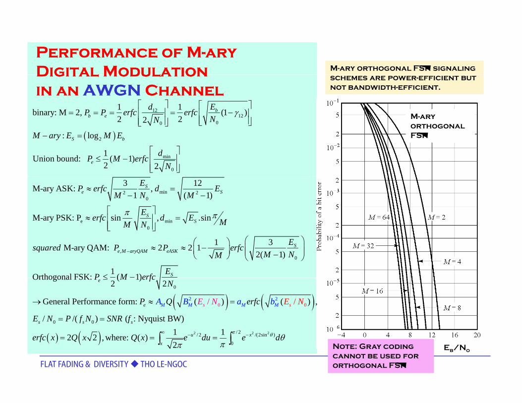
Performance of MPerformance of M--aryaryDigital Modulation Digital Modulation M-ary orthogonal FSK signaling Digital Modulation Digital Modulation in an in an AWGNAWGN ChannelChannel

schemes are power-efficient but not bandwidth-efficient.

1212

00

1 1binary: M 2, (1 )2 22

bb e

EdP P erfc erfcNN

γ⎡ ⎤ ⎡ ⎤

= = = = −⎢ ⎥ ⎢ ⎥⎢ ⎥⎢ ⎥ ⎣ ⎦⎣ ⎦

M-ary orthogonal

( )2

min

0

: log

1Union bound: ( 1)2 2

S b

e

M ary E M E

dP M erfcN

⎣ ⎦⎣ ⎦− =

⎡ ⎤≤ − ⎢ ⎥

⎢ ⎥⎣ ⎦

orthogonal FSK

min2 20

e0

3 12M-ary ASK: ,1 ( 1)

M-ary PSK: P sin

Se S

S

EP erfc d EM N M

EerfcM Nπ

≈ =− −

⎡ ⎤≈ ⎢

⎢⎣ ⎦min, .sinSd E M

π=⎥⎥0M N⎢⎣ ⎦

,0

1 3M-ary QAM: 2 2 12( 1)

1Orthogonal FSK: ( 1)

Se M aryQAM eASK

S

Esquared P P erfcM NM

EP M erfc

−

⎥

⎛ ⎞⎛ ⎞≈ ≈ − ⎜ ⎟⎜ ⎟ ⎜ ⎟−⎝ ⎠ ⎝ ⎠

≤ −

( ) ( )2 2

0

0

0

0

0

Orthogonal FSK: ( 1)2 2

General Performance for /m: ( ) ( ) ,

/ /( )

/M M M Me ss

e

s s

P M erfcN

P Q er Efc

E N P

A B aE N

f SN

b N

N

≤

→ ≈ =

= = ( : Nyquist BW)sR f

FLAT FADING & DIVERSITY THO LE-NGOC

Eb/NoNote: Gray coding cannot be used for orthogonal FSK

( ) ( ) 2 2 2/ 2/ 2 /(2sin )

0

1 12 2 , where: ( )2

u x

xerfc x Q x Q x e du e d

π θ θππ

∞ − −= = =∫ ∫

PROBABILITY OF PROBABILITY OF SYMBOL ERRORSYMBOL ERROR

M-QAM, M-PSK: BW-efficient but not power-efficientSYMBOL ERRORSYMBOL ERROR For M>8, M-QAM outperforms M-PSK

MPSKMQAM


Eb/No Eb/No

EXAMPLE OF BPSK PERFORMANCEEXAMPLE OF BPSK PERFORMANCE

[ ] [ ] [ ] where [ ] with prob. of 1/2, r k x k w k x m a= + = ±

AWGN channel:

E o p obabilit deca s e ponentiall

( )2

- /e

and [ ]: Gaussian (0, / 2)

P = 2 / 0.5 b o

b b o

E Nb o

E a T w m N

Q E N e

=

≈Needs to increase this slope by diversity

Error probability decays exponentiallywith SNR

[ ][ ] [ ] [ ]r k x k w kh k= +Rayleigh Flat-Fading Channel:

techniques

( )2

[ ]s

[ ]

[ ] : Rayleigh wit

[ ] [

h

] [ ]

1,

P = 2 /[ ]h k b o

r k x k w k

Q E N

h k

h

k

k

h

σ

= +

=slope=-1

b bili

( )[ ][ ] [ ]

/1 112 1 / 4 /s

b o

b o b o

E NP

E N E N

⎛ ⎞⎜ ⎟= − ≈⎜ ⎟+⎝ ⎠

FLAT FADING & DIVERSITY THO LE-NGOC 4

average error probability decays only inversely with SNR

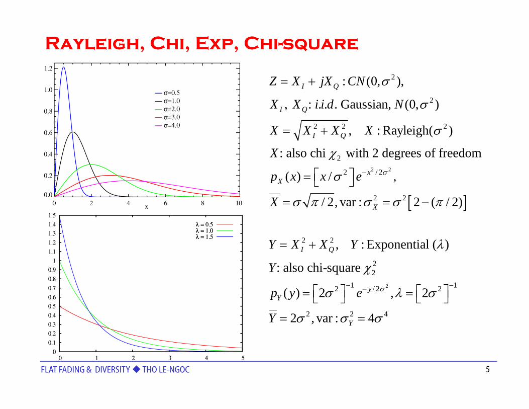
Rayleigh, Chi, Exp, ChiRayleigh, Chi, Exp, Chi--squaresquare

22

2

2 2 2

: (0, ),

, : . . . Gaussian, (0, )

R l i h( )

I Q

I Q

Z X jX CN

X X i i d N

X X X X

σ

σ

= +

2 2

2 2 2

2

2 / 2

, : Rayleigh( )

: also chi with 2 degrees of freedom

( ) /

I Q

x

X X X X

X

p x x e σ

σ

χ

σ −

= +

⎡ ⎤= ⎣ ⎦

[ ]2 2

( ) / ,

/ 2, var : 2 ( / 2)

X

X

p x x e

X

σ

σ π σ σ π

⎡ ⎤⎣ ⎦

= = −

2 2 , : Exponential ( )

: also chi-I QY X X Y

Y

λ= +22square χ

21 12 / 2 2

2 2 4

( ) 2 , 2

2 , var : 4

yY

Y

p y e

Y

σσ λ σ

σ σ σ

− −−⎡ ⎤ ⎡ ⎤= =⎣ ⎦ ⎣ ⎦= =


RiceanRicean2

2 2 2

, : Gaussian with same variance, ( , ), ,

: Ricean ( ),

I Q i

I Q

X X independent N i I Q

X X X

μ σ

σ

=

= +

( )2 2 2/ 22 20

2 2 2 2 2 2 2

( ) / ( / ) ,

, / 2 , { } 2 ,

x sX

I Q

p x x I sx e

s s E X s

σσ σ

μ μ κ σ σ

− +⎡ ⎤= ⎣ ⎦

= + = = +

2/ 2

0 1{ } (1 ) ( ) ( )2 2 2

E X e I Iκ πσ κ κκ κ− ⎡ ⎤= + + +⎢ ⎥⎣ ⎦

Bessel

2

function of the 1st kind and order :

( ) ( / 2) /[ ( 1) !]a ka

a

I y y a k k∞

+= Γ + +∑ ( )0

2

00

( ) /(2 !)

k

k k

kI y y k

=

∞

=

⎡ ⎤→ = ⎣ ⎦

∑

∑

( )Xp x


x

Gaussian, Chi, ChiGaussian, Chi, Chi--squaresquare

2

2

, 1,2,..., : independent : ( , )i i i

k

X i k Gaussian N μ σ=

⎡ ⎤

2

1

1/ 2 1 1 / 2

:

( ) 2 ( / 2)

ki i

Ki i

k k x

XX

p x k x e

μ χσ=

−− − −

⎡ ⎤−= ⎢ ⎥

⎣ ⎦

⎡ ⎤= Γ⎣ ⎦

∑

{ } [ ]( )/ 2

2

( ) 2 ( / 2) ,

2 / 2 ( / 2),

X

n n

k

p x k x e

E X k n k

X

⎡ ⎤= Γ⎣ ⎦

= Γ + Γ

⎡ ⎤ 2

1

1/ 2 / 2 1 / 2

:

( ) 2 ( / 2) ,

ki i

Ki i

k k yY

XY

p y k y e

μ χσ=

− − −

⎡ ⎤−= ⎢ ⎥

⎣ ⎦

⎡ ⎤= Γ⎣ ⎦

∑

( ) 2 ( / 2) ,

, var :

Y

Y

p y k y e

Y k σ

⎡ ⎤Γ⎣ ⎦= 2 2k=


Gaussian, Chi, ChiGaussian, Chi, Chi--squaresquare2, 1,2,..., : i.i.d. Gaussian: (0, )iX i K zero mean N σ= −

2 : chi with degrees of freedomK

i KX X Kχ= ∑

{ } [ ]( )2

2 2

2

1

1 / 2/ 2 1 1 / 2 2

2 / 2case =2:

( ) 2 ( / 2

Rayleigh ( )

) , 2 / 2 ( / 2) ,

i

nK K K x n

x

Xp x K x

K p x xe

e E X K n Kσ

σσ

σ σ

=

−− − −

− −

⎡ ⎤ ⎡ ⎤= Γ = Γ + Γ⎣ ⎦ ⎣ ⎦

{ } { }2 2 2/ 2 2E X E X σπσ ⎡ ⎤⎣ ⎦case =2: Rayleigh, ( ) ,XK p x xeσ= { } { }2 2

1

/ 2, 2

: chi-square with degrees of freedomK

i Ki

E X

Y X K

E X

χ

σπσ

=

=

⎡ ⎤= = ⎣ ⎦

∑2

2

1/ 2 / 2 1 / 2

12 / 2 2 2

2 2 4

4case =2: exponential, ( ) 2 , 2 , var :

( ) 2 ( / 2) , , var : 2

4

K K K

Y

y

yY

Y Yp y K y e Y K K

eK p Yy

σ

σ

σ

σ σ σ σ

σσ σ−

−

− −

−

⎡ ⎤= Γ = =⎣ ⎦

⎡ ⎤= =⎣ ⎦ =

1( )

Y

u

Y

u t e−=

⎣ ⎦

Γ0

, 0, ( 1) ( ), (1/ 2) ,tdt u u u u π∞ − > Γ + = Γ Γ =∫


0

(2) (1) 1, ( ) ( 1)! for : integer 1n n nΓ = Γ = Γ = − >∫

NakagamiNakagami mm--distribution:distribution:V N k i di t ib t d

( ) 22 1 /

2 2 2 2

V: Nakagami m-distributed:

( ) 2 / / ( )

{ }, {[ ] } /

m m mvVp v m m v e

E V E V m

− − Ω⎡ ⎤= Ω Γ⎣ ⎦Ω = −Ω = Ω

1

{ }, {[ ] } /0.5 : fading figure,ratio of moments.

{ } ( / ) ( 0.5) / ( )

E V E V mm

E V m m m∞

Ω Ω Ω≥

= Ω Γ + Γ

∫( )Vp v

1

0( ) , 0,

( 1) ( ), (1/ 2) ,(2) (1) 1,

u tu t e dt u

u u u π

∞ − −Γ = >

Γ + = Γ Γ =Γ = Γ =

∫

( ) ( ) ,(nΓ

{ } { }

2 22 / 2

2 2 2

1 : Rayleigh,

) ( 1)!for : intege

(

r 1

) xXm X p x x

n

e

nσσ − −= → =

⎡ ⎤

= − >

v{ } { }2 2 22 , / 2E X XEσ πσ⎡ ⎤= =⎣ ⎦

pdf converges to a delta function for increasing m.matched empirical results for short wave ionospheric propagation.


matched empirical results for short wave ionospheric propagation.

Diversity Approach Diversity Approach for frequencyfor frequency--flat fading channelsflat fading channelsfor frequencyfor frequency flat fading channelsflat fading channels

ER

(S

) RECEIVER 1

TY

E

R

ER

FF fading channel 1

TR

AN

SM

ITT

E

RECEIVER 2

RECEIVER L

DIV

ER

SIT

CO

MB

INE

DE

CO

DE

FF fading channel L

FF fading channel 2

••• ••

•

••

•

Multiple independent paths (or channels) unlikely to fade simultaneously

Multiple independent paths (or channels) unlikely to fade simultaneously

channel L

simultaneously

⇒ Diversity techniques:Send the same signals over independentfading paths obtained by diversity in

simultaneously

⇒ Diversity techniques:Send the same signals over independentfading paths obtained by diversity in

Complex baseband

FF fading channel l

ljl lh h e ϕ=

fading paths obtained by diversity in time, space, frequency, …

⇒ reduced possibility of all paths in deep fading simultaneously

fading paths obtained by diversity in time, space, frequency, …

⇒ reduced possibility of all paths in deep fading simultaneously

WGN, wl


p g yCombine paths to mitigate fading effects

p g yCombine paths to mitigate fading effects

DIVERSITY SCHEMESDIVERSITY SCHEMES

Time diversity (1 Tx+ 1 Rx):multiple transmission of the same information over different time slotsinformation over different time slotstime separation > channel coherence time

Frequency diversity (L Tx + L Rx):multiple transmission of the same information over different frequency slotsfrequency separation > channelfrequency separation > channel coherence bandwidth

Space diversity (1-L Tx + 1-L Rx):transmission to multiple antennasS ffi i t t ti tSufficient antenna separation to achieve uncorrelated channel gains, e.g., about half wavelength, λ/2, for a Rayleigh fading channel.


a Rayleigh fading channel.

Diversity Techniques at ReceiverDiversity Techniques at ReceiverTransmitter sends the same signals over L independent fading paths obtained by diversity in time space frequency : Simplest Coding: Repetitiondiversity in time, space, frequency, …: Simplest Coding: Repetition

[ ] [ ][ ]

( ) ( )( ) ( ), ( ) ( ), 1,.., ,

( ) ( ), 1,.., ( ) : . .

, 1,..,

.

( ) Tl

Tl

Tl l

k h k lk k k y k l L

k n k l L n k i i d AW

Lx

GN

k= + = ==

= =

=hy n y

n

h

x(t)1jh h ϕ

R

[ ]( ) ( ), , , ( )l l

Receiver combines paths to mitigate fading effectsclassic vector detection in white1

1 1jh h e ϕ=

22 2

jh h e ϕ= MB

INE

R classic vector detection in white Gaussian noiseDiversity gain is indicated by changes in BER slope

Combining Techniques:2 2

33 3

jh h e ϕ=E

AR

CO

M

Maximal Ratio Combining (MRC): all paths cophased and summed with optimal weights to maximize combiner output SNREqual Gain Combining (EGC):

LIN

E Equal Gain Combining (EGC):All paths co-phased and summed with equal weightsSelection Combining (SC):select the fading path with the hi h t i


LjL Lh h e ϕ=

highest gain

Selection Selection combiningcombining over Rayleigh fadingover Rayleigh fading

1 2( )received vector: ( ) ( ), [ , ,..., ]TLx kk k h h h= + =n hr h

212 2 / 2 2 2 4

: . . ., RaRayleigh channel: , 1, 2, yleigh.., :

0 : exponential, ( ) 2 , 2 , var : 4

ljl l l

yl Y Y

L i i dh h e l h

Y h p y e Y

ϕ

σσ σ σ σ− −

= =

⎡ ⎤= > = = =⎣ ⎦

*select the max and coh er n ly e th

{ }* **( ) ( ), max , 1,2,..,

demodulate:

( ) lx kr k n k h l Lh h= + ==%

{ }{ }

2 212 / 2

0

2*

2

2

1

cdf:Pr Pr

Pr

2L

ll

Ly xe dx

d

y h y

y

h

h

σσ=

− −⎡ ⎤⎡ ⎤= ⎣ ⎦⎢⎧ ⎫

≤ = ≤⎨ ⎬⎩ ⎭ ⎥⎣ ⎦

≤

∫I

{ }

[ ]

2

2*

2* / 22

2*

1/ 2

Pr, 0

2

/ as compared to non-divers

( ) 1y

SC s o

h

Ly

d Lp y ey

e y

SNR E

h

N

dy

h

σ σ

σ−

−−⎡ ⎤= = −

≤≥

=

⎣ ⎦

[ ]2ity case: /l s oSNR h E N=[ ]* pSC s o [ ]

( )*

2 2 1/ 22 / 2

2*

y

BPSK: = 2 /

L

l s o

bh osP Q E Nh

−∞ ⎡ ⎤

⎛ ⎞⎜ ⎟⎝ ⎠

⎡ ⎤ ∫solved by numerical


( ) 2 2/ 22 / 2

0/(2 ) 2 / 1s

yo

ybP L Q E N e ye dy σ σσ −∞ − ⎡ ⎤−⎣⎡ ⎦⎤→ = ⎣ ⎦ ∫

solved by numerical integration

Selection Combining (SC) Diversity in Rayleigh channelsSelection Combining (SC) Diversity in Rayleigh channels

212 2 /2 2 2 4

Rayleigh channel: , 1,2,.., :

0 : exponential, ( ) 2 , 2 ,var : 4

: . . ., Rayleighljl l l

yl Y Y

h h e l h

Y h p y e Y

L i i dϕ

σσ σ σ σ− −

= =

⎡ ⎤= > = = =⎣ ⎦

{ }*

*

* *( )

se

( ), max , 1,2

lect th

,.

coherentle max and demodulatey

.( )

:

, l

h

h hx kr k n k h l L+ == =%

2 2 1/ 2/ 2

LL −⎡ ⎤2

2

2*

2

2

2

/ 2

1/ 2

/ 22

1*

1

2 / 2 2 2

0

, 02

{ /(2 ) (2 ) (1 2 )}

( ) 1h

L

y

Lyy

l

ye y

E L

Lp y

ye dyh

e

le

σσ

σσ

σ

σ σ σ

−

−

−

−−∞ −

≥

⎡ ⎤ =⎣

⎡ ⎤= −⎣ ⎦

⎡ ⎤−⎣ ⎦= ⎦ ≥∫ ∑( )p y 1l=2*

( )h

p yIncreased average path gain by a factor (1+1/2+1/3+…+1/L)This factor is reduced with large L.


y14

SelectionSelection combining: performance ofcombining: performance of BPSK over BPSK over Rayleigh fadingRayleigh fading

( ) 22

*

1/2

*2 / 2

0

2BPSK: = 2 / /(2 ) 12 /sy

b o b

Ly

h osP Q E N P L Q E N e dyeh y σ σσ∞ −

− −⎛ ⎞ ⎡ ⎤→ =⎜ ⎟ ⎣ ⎡ ⎤−⎣ ⎦⎦⎝ ⎠ ∫

gain is reduced with large L.

⎝ ⎠

Pb

FLAT FADING & DIVERSITY THO LE-NGOC 15Eb/No

EGC EGC & its Performance & its Performance in Rayleigh Channelsin Rayleigh Channels

received vector: ( ) ( ),Rayleigh channel: , 1, 2,.., :

( ): . . ., Rayleighlj

l l l

k kh h e l h

x kL i i dϕ

= +

= =

hr n

212 2 / 2 2 2 40 : exponential, ( ) 2 , 2 , var : 4

demodulate and combine with weigh

yl Y YY h p y e Y

Coherently equal

σσ σ σ σ− −⎡ ⎤= > = = =⎣ ⎦

1 2ts: [ , , 2,.., ]Lj j je e eϕ ϕ ϕ− − −

⎡ ⎤

=hΦ

[ ] [ ]1

22

( ) ( ) ( ), , ( ) ( ) : (0, / 2)

/ as compared to non-diversity case: /

( )

/

L

sum sum l ol

EGC l

r k k h w k h h w k k Gaussian LN

SNR E N SNR h E Nh L

x k=

⎡ ⎤= = + = =⎢ ⎥

⎣ ⎦

=⎡ ⎤⎣ ⎦=

∑h hΦ Φr n%

[ ] [ ]

2

/ as compared to non diversity case: /

BPSK: =

/

2

sumEGC s o l s o

bh sus m

SNR E N SNR h E Nh L

hP Q E

⎡ ⎤⎣ ⎦

( )/ oNsum bh sus m( )o


Average BER of BPSK over Average BER of BPSK over NakagamiNakagami--m fading m fading channels with MRC and channels with MRC and EGC EGC (L = 4(L = 4).).

Pb


From Marvin K. Simon and Mohamed-Slim Alouini, Digital Communication over Fading Channels, 2nd Edition, John Wiley & Sons, 2005

Eb/No

MRC & its Performance MRC & its Performance in Rayleigh Channelsin Rayleigh Channels

212 2 / 2

1 2( )

: . . ., Ra

received vector: ( ) ( ),

Rayleigh channel: , 1,2, yleigh

[ , ,..., ]

.., :

0 : exponential, ( ) 2

ljl l l

yl

T

Y

Lx k

L i i d

k k

h h e l

h h h

h

Y h p y e

ϕ

σσ− −

= +

=

=

=

⎡ ⎤= > = ⎣ ⎦

h hr n

2 2 4

*sele

0 : exponen

ct

tia

the max

l, ( ) 2

2 , var : 4

coherentand l dy

l Y

Y

h

Y h p y e

Y

σ

σ σ σ

⎡ ⎤> ⎣ ⎦= =

2 2

emodulate and combine with optimum weights, :Hh

[ ] [ ]2 2

2 2( ) ( ) ( ), ( ) ( ) : (0, / 2)

instantaneous / as compared to non-diversity case

matched filt ( )er:

: /

o

EGC s o l s o

H Hr k k w k w k k Gaussian N

SNR E

x k

N SNR h E N

= = + =

= =⎡ ⎤⎣ ⎦

h h h

h

r n h%

212 1 / 2 2 2 42 L L L−⎡ ⎤

max output SNR

Y =212 1 / 2 2 2 42

2

( ) 2 ( 1)! , 2 , var : 4

BPSK: = 2 /

, L L L yY Y

b os h

p y L y e Y L

P Q E N

Lσσ σ σ σ− −⎡ ⎤= − = =⎣ ⎦⎛ ⎞⎜ ⎟⎝ ⎠

h

h

( )[ ][ ]

212 1 / 2

0

21

2

2 ( 1)! 2 /

1 2 /1 1 ,2 2 1 2 /

s

s

L L L yb o

L lLb o

P L Q E N y e dy

L l

y

E NP

l E N

σσ

σγ γ γσ

∞− − −

−

⎡ ⎤→ = −⎣ ⎦

− +⎛ ⎞− +⎡ ⎤ ⎡ ⎤= =⎜ ⎟⎢ ⎥ ⎢ ⎥ +⎣ ⎦ ⎣ ⎦⎝ ⎠

∫

∑


[ ]02 2 1 2 /l obl E Nσ=⎢ ⎥ ⎢ ⎥ +⎣ ⎦ ⎣ ⎦⎝ ⎠

18

Performance of BPSK using Performance of BPSK using MRC in Rayleigh ChannelsMRC in Rayleigh Channels

[ ]

[ ]

2

2

for 2 / 1,11 ,

4 /

b oE N

E N

σ

γσ

>>

≈ −

sP

[ ]

[ ]2

1

4 /11 2,1 ,

4 /

1 2 1

b o

b o

L

E N

E N

L l L

σ

γ γσ

+ ≈ − ≈

⎛ ⎞ ⎛ ⎞1

0

1 2 1

2 1 1

L

l

L

L l Ll L

LP

−

=

− + −⎛ ⎞ ⎛ ⎞=⎜ ⎟ ⎜ ⎟

⎝ ⎠ ⎝ ⎠

⎡ ⎤−⎛ ⎞→ ≈ ⎢ ⎥⎜ ⎟

∑

[ ]24 /s

b o

PL E Nσ

→ ≈ ⎢ ⎥⎜ ⎟⎢ ⎥⎝ ⎠ ⎣ ⎦


[ ]/b oE N

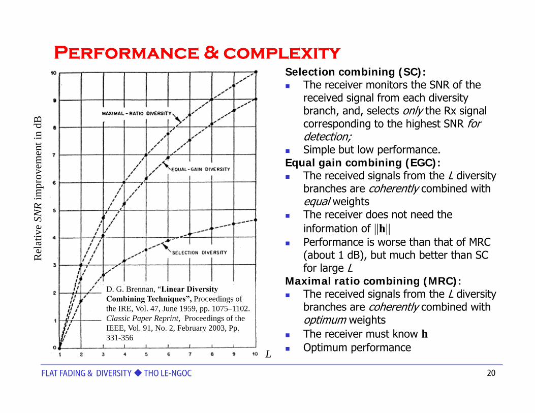
Performance & complexityPerformance & complexitySelection combining (SC):g ( )

The receiver monitors the SNR of the received signal from each diversity branch, and, selects only the Rx signal corresponding to the highest SNR for dB p g gdetection;Simple but low performance.

Equal gain combining (EGC):The received signals from the L diversity ro

vem

ent i

n

g ybranches are coherently combined with equal weightsThe receiver does not need the information of ||h||ve

SN

Rim

pr

|| ||Performance is worse than that of MRC (about 1 dB), but much better than SC for large L

Maximal ratio combining (MRC):

Rel

ativ

a a at o co b g ( C)The received signals from the L diversity branches are coherently combined with optimum weightsThe receiver must know h

D. G. Brennan, “Linear Diversity Combining Techniques”, Proceedings of the IRE, Vol. 47, June 1959, pp. 1075–1102. Classic Paper Reprint, Proceedings of the IEEE, Vol. 91, No. 2, February 2003, Pp. 331 356


The receiver must know hOptimum performanceL

331-356

Diversity Diversity techniques intechniques in

LOS SystemsLOS Systems


DiversDiversiityty improvement in LOS Systemsimprovement in LOS Systems

improvement in dB for fading>20dBimprovement in dB for fading 20dB

SPSPAACE DIVERSCE DIVERSIITY TY (A. Vigants): ISD=(1.2E-3)(S2f/d) .10-ΔG/20 10F/10

S = vertical separation of equal size antennas in metersf = frequency in GHzf frequency in GHzΔG = effective gain difference between the two antennas, due either to different sizesor different waveguide run losses, referenced to the basic path reliability calculationsF = median fade depth in decibelsF median fade depth in decibelsd = path length in kilometersFor the specular reflection or overwater problem, one alternative is to select the antenna separation on the receive terminal for S =246d/fhtS = antenna separation in metersS antenna separation in metersd = path length in kilometersf = frequency in GHzht = heights of the transmitter antenna above the water in meters

FREQUENCY DIVERSITY FREQUENCY DIVERSITY ( W.T. Barnett): IFD = 10log [ K 10F/10 Δf/f]Δf = difference between two RF carriers, in GHzf = RF carrier in GHzK=(1.1)10-a, a=log(f0.8), empirically derived frequency-dependent constant


( ) , g( ), p y q y pF = multipath fade depth in dB, normally set equal to equipment fade margin

Capacity of Capacity of AWGNAWGN ChannelChannel( ) ( ) ( ) ( ) :y k x k n k n k AWGN= +

20 0 0

( ) ( ) ( ), ( ) :

Capacity: log 1 / / ,b b

y k x k n k n k AWGN

E EC C C P SNRB N B N B N B

b s Hz

= +

⎛ ⎞⎛ ⎞ ⎛ ⎞ ⎛ ⎞= + = =⎜ ⎟⎜ ⎟ ⎜ ⎟ ⎜ ⎟⎝ ⎠ ⎝ ⎠ ⎝ ⎠⎝ ⎠

⎧( ) 2

02

2

log , 0log 1

log , 1

P e for SNRNC B SNR

B SN or SNR f R

⎧ ≈⎪⇒ = + ≈ ⎨⎪ >>⎩

20

log PC eN

≤ →

2

POWER-LIMITED REGION

SNR<<1, log PC e≤CAPACITY IN

ity,

C2

0

, gN

POWER-LIMITED REGION: linear in power,

insensitive to bandwidth

Ca

pa

ci

20

BANDWIDTH-LIMITED REGION

C/B<<1, SNR>>1, log 1 PC BN B

⎛ ⎞= +⎜ ⎟

⎝ ⎠

• BANDWIDTH-LIMITED REGION: • logarithmic in power,

• approximately linear in bandwidth


Bandwidth B

FrequencyFrequency--flat fading channel capacityflat fading channel capacity::

Theoretical limit on maximum error-free Tx rate a channel can support due to channel characteristics and not dependent on design techniquesIt depends on what is known about channel fading.

No knowledge: Worst-case channel capacity

Partial knowledge of fading statisticsFull knowledge of fading level at receiver only

( )2 2log 1 ( ) log (1 )C B aSNR p a da B aSNR∞

= + ≤ +∫ (using Jensen’s inequality)

0

Full knowledge of fading level at both transmitter and receiver:For fixed transmitted power, same as above

transmit power can be adapted to a for optimum results

( )2( ) [ ( )]0

max log 1 ( ) ( )SNR a E SNR a SNR

C B aSNR a p a da∞

== +∫

transmit power can be adapted to a for optimum results


0

Slow FlatSlow Flat--Fading ChannelsFading ChannelsFading Known at Fading Known at Receiver Receiver

( ) ( )

2

2

( ) ( ) ( ), ( ) : , power fading with

instantaneous: ( ) ( ) ( ) log 1 /

: pdf ( )y k x k n k n k AWGN

P a A Q B aSNR C a B aSNR b s

h a h p a== +

≈ = +( ) ( )2instantaneous: ( ) ( ) , ( ) log 1 / ,

Performance outage probability:

s M MP a A Q B aSNR C a B aSNR b s≈ = +

For Slow Fading: Tsymbol<< Tcoherence

PPsTARGET

OUTAGE

{ } { }Performance outage probability:

Pr ( ) PrTP s sTARGET TARGETO P a P a a= > = <

Ps

TIME

Capacity outage probabil

( ){ }2

ity:

Pr log 1TC TO B aSNR C= + ≤ 10%

TCO =/C C

[ ] 1/2 1T

T

C BCO SNR −⎡ ⎤≈ −⎣ ⎦

( )2log 1AWGNC B SNR= +

( ){ }

[ ]

1/2

1/

for a : Rayleigh-distributed,

2 1

T

T

T

C BCO SNR −⎡ ⎤≈ −⎣ ⎦

1%TCO =

/T AWGNC C


[ ]TC ⎣ ⎦

Receive Diversity: Capacity Receive Diversity: Capacity Outage ProbabilityOutage ProbabilityOutage ProbabilityOutage Probability

( ){ }22

Capacity outage probability:

Pr log 1C TO B SNR C= + ≤h( ){ }2ogTC TO SN C

/C C/T AWGNC C


Fast FlatFast Flat--Fading ChannelsFading ChannelsFading Known at Fading Known at Receiver Receiver

( ) ( )2

2( ) ( ) ( ), ( ) : , power fading with: pdf

i ( ) ( ) ( ) l

( )

1 /

h a h p ay k x k n k n k AWGN

P A Q B SNR C B SNR b

+ ==

( ) ( )22instantaneous: ( ) ( ) , ( ) log 1 / ,s M MP a A Q B aSNR C a B aSNR b s= +≈

For Fast Fading, Tsymbol ≈ Tcoherence or > Tcoherence, introduced random phase can remove correlation between symbolintroduced random phase can remove correlation between symbol phases, and hence leads to an irreducible error floor for differentialmodulation/demodulation.For coherent demodulation, if fading is known by receiver only:

( ){ } ( ) ( )ergodic: log 1 ( ) log 1C E C a B aSNR p a da B SNR∞

= = + ≤ +∫

For coherent demodulation, if fading is known by receiver only:

0

verage (symbol) error probability: ( ) ( )s sP P a p a da∞

= ∫A

i.e., If Fading Known at Receiver

( ){ } ( ) ( )2 20ergodic: log 1 ( ) log 1C E C a B aSNR p a da B SNR= = + ≤ +∫

(using Jensen’s inequality)


Only, at best, ergodic C approaches CAWGN

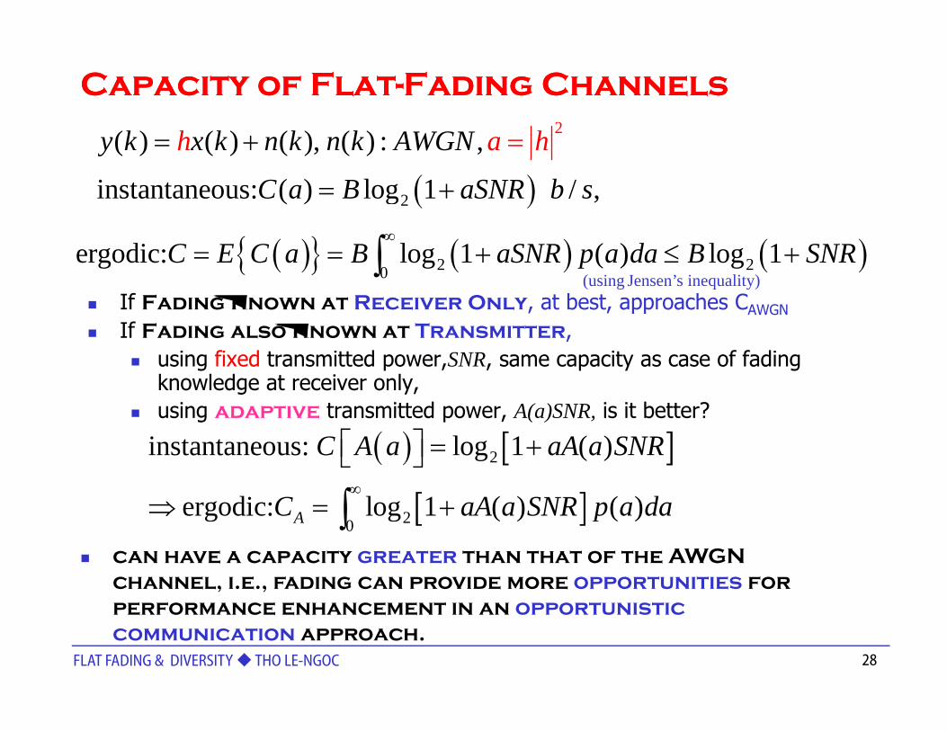
Capacity of FlatCapacity of Flat--Fading ChannelsFading Channels2( ) ( ) ( ) ( )k k k k AWGN hh

( )2

( ) ( ) ( ), ( ) : ,

instantaneous: ( ) log 1 / ,

y k x k n k n k AWGN

C a B aSNR

a h

b s

h= + =

= +

If Fading Known at Receiver Only, at best, approaches CAWGN

( ){ } ( ) ( )2 20ergodic: log 1 ( ) log 1C E C a B aSNR p a da B SNR

∞= = + ≤ +∫

(using Jensen’s inequality)

If Fading also Known at Transmitter, using fixed transmitted power,SNR, same capacity as case of fading knowledge at receiver only,using adaptive transmitted power A(a)SNR is it better?using adaptive transmitted power, A(a)SNR, is it better?

( ) [ ]

[ ]2instantaneous: log 1 ( )

ergodic: log 1 ( ) ( )

C A a aA a SNR

C aA a SNR p a da∞

⎡ ⎤ = +⎣ ⎦

⇒ +∫ [ ]20ergodic: log 1 ( ) ( )AC aA a SNR p a da⇒ = +∫

can have a capacity greater than that of the AWGN channel, i.e., fading can provide more opportunities for


performance enhancement in an opportunistic communication approach.

FlatFlat-- Fading Also Known at Transmitter:Fading Also Known at Transmitter:using using AdaptiveAdaptive Channel InversionChannel Inversion

Channel Inversion: A(a)=1/a to maintain a constant SNRZO for zero outage(e.g., same as perfect power control in CDMA) under average Tx power constraint : ( g , p p ) g p

Simplifies design (i.e., fixed rate at all channel states) but is power-inefficient since for very small a, A(a)=1/a is very large.

( ) ( ) [ ] [ ]1/ l 1 ( ) l 1A C A A S S⎡ ⎤( ) ( ) [ ] [ ]

( ){ } { }2 2

0

=1/ log 1 ( ) log 1

but with Tx power constraint: ( ) ( ) =1 1/

ZO ZOA a a C A a aA a SNR SNR

A a p a da E A a E a∞

⎡ ⎤→ = + = +⎣ ⎦

→ =∫[ ] { }2ergodic, zero-outage: log 1 with =

1/ZO ZO ZOSNRC SNR SNR

E a⇒ = +

Greatly reduces capacity:Capacity is zero in Rayleigh fading since E{a-1} →∞Greatly reduces capacity:Capacity is zero in Rayleigh fading since E{a } →∞achieves a delay-limited capacity.

Truncated inversion: A(a)=1/a only if a is above cutoff fade depthto maintain constant SNR (and hence fixed rate) above cutoff


to a ta co sta t S (a d e ce ed ate) abo e cutoto increase capacity with appropriate choice of cutoff: Close to optimal

FlatFlat-- Fading Also Known at Transmitter:Fading Also Known at Transmitter:

using using Optimal Adaptive Tx powerOptimal Adaptive Tx power

( ) [ ]2 0instantaneous: log 1 ( ) with Tx power constraint: ( ) ( ) =1C A a aA a SNR A a p a da

∞⎡ ⎤ = +⎣ ⎦ ∫

[ ]{ }

[ ]2 ,max 20 ( ): ( ) 10

ergodic: log 1 ( ) ( ) max log 1 ( ) ( )

1 1l ti ( ) l t f

A A A a E A aC aA a SNR p a da C B aA a SNR p a da

A

∞∞

=⇒ = + ⇒ = +

+⎡ ⎤⎢ ⎥

∫ ∫

( )T t i t l / ( )C B SNR d∞

∫1 1solution: ( ) select fooo

A a aa a⎡ ⎤= −⎢ ⎥⎣ ⎦

( )2r Tx power constraint log / ( ) .o

oa

C B aSNR a p a daA⇒ = ∫1a

1 1( )o

A a a a

+⎡ ⎤= −⎢ ⎥⎣ ⎦

1select for Tx power constraint,oo

a a →( ) 0A a =

Waterfilling and rate adaptation:g ptransmit more when channel is good with separate coding for each fading statemaximize long-term throughput


g g pbut incur delay.

Waterfilling:Waterfilling: Performance Performance Waterfilling:Waterfilling: Performance Performance

at low SNR • Waterfilling provides a significant

power gainpower gain./a AWGNC C

at high SNR,• waterfilling does not provide any

gain but

/aC B

gain, but• CSI allows rate adaptation and

simplifies coding.


Adaptive ModulationAdaptive ModulationAdaptive ModulationAdaptive ModulationAdapt modulation to fading

Parameters: Constellation size, Tx power, AMCOptimization criterion: Max throughput, minimum BER, or minimum Tx power. p g p , , pExample: Rate and Power Optimization to max rate for a target BER

[ ]coherent M-QAM in AWGN for 4,0 30 : 0.2exp 1.5 /( 1) , in presence of fading , for a target , select ( )

b

b

M SNR dB P SNR Ma P A a

≥ ≤ ≤ ≤ − −

→

{ }{ }

{ }2 2( ): ( ) 1 ( ): ( ) 1

1.5max log [ ( )] max log 1 ( )ln(5 )A a E A a A a E A a

b

SNRE M a E aA aP= =

⎧ ⎫⎡ ⎤⎪= −⎨ ⎢ ⎥⎪ ⎣ ⎦⎩

0ln(5 ) ln(5 )1 b bP a P

⎪⎬⎪⎭

⎧ + ≥⎪ 0( ) ( )11.5 1.5( )

0 else

1.5log ( )

b b

oa a aA a

aC B p a da∞

⎧ + ≥ −⎪= ⎨⎪⎩

⎛ ⎞−= ⎜ ⎟∫ 2

ln(5 ) /1.5

log ( )ln(5 )

o b

opto ba P

C B p a daa P−

= ⎜ ⎟⎝ ⎠

∫Pb=1E-3 Pb=1E-6

Shannon limit


cy ff fading & diversity - mcgill university

Documents