Cyclical Implications of the Basel-II Capital Standards

Anil K Kashyap Graduate School of Business, University of Chicago

Jeremy C. Stein

Department of Economics, Harvard University

November 2003

We are grateful to Sebastian Fritz, Michael Luxenburger and Peter Garber of Deutsche Bank for their contributions to this project. Thanks also to Jon Frey, Craig Furfine, Eric Rosengren, Vicky Saporta and seminar participants at the Federal Reserve Bank of Chicago for helpful comments and suggestions.

1

I. Introduction

One of the central pillars of the new Basel-II regulatory framework is the concept

of risk-based capital requirements.1 Under the so-called IRB (internal-ratings-based)

approach, the amount of capital that a bank will have to hold against a given exposure

will be a function of the estimated credit risk of that exposure. Estimated credit risk in

turn is taken to be predetermined function of four parameters: probability of default (PD);

loss given default (LGD); exposure at default (EAD); and maturity (M). Banks operating

under the “Advanced” variant of the IRB approach will be responsible for providing all

four of these parameters themselves, based on their own internal models. Banks

operating under the “Foundation” variant of the IRB approach will be responsible only

for providing the PD parameter, with the other three parameters to be set externally, by

the Basel committee.2

It is clear that there are many potential benefits to risk-based capital requirements.

As compared to the “one-size-fits-all” approach embodied in the original Basel-I

framework, risk-based capital requirements should reduce pricing distortions across loan

categories, as well as the accompanying incentives for banks to engage in various forms

of regulatory capital arbitrage. At the same time, this new approach to capital regulation

raises some concerns. One concern which has been repeatedly voiced—but which has

been subject to relatively little formal analysis—is that the new capital standards will

exacerbate business-cycle fluctuations. In brief, the idea is that in a downturn, when a

1 For an overview of the Basel-II accord, see Basel Committee on Banking Supervision (2003). 2 See Jackson (2002) for an explicit description of the Basel committee’s capital-requirement formula, and its evolution over time.

2

bank’s capital base is likely being eroded by loan losses, its existing (non-defaulted)

borrowers will be downgraded by the relevant credit-risk models, forcing the bank to

hold more capital against its current loan portfolio. To the extent that it is difficult or

costly for the bank to raise fresh external capital in bad times, it will be forced to cut back

on its lending activity, thereby contributing to a worsening of the initial downturn.

Our aim in this paper is to take a closer look at this “cyclicality” aspect of the

Basel-II capital regulations. There are two primary components to our analysis. First, we

start by developing a conceptual framework which can be used to ask questions about the

optimality of the proposed regulations. Our main conclusion here is that the Basel-II

approach of having a single time-invariant “risk curve”—that maps credit-risk measures

(such as the PD) into capital charges—is, in general, sub-optimal. From the perspective

of a social planner who cares not just about bank defaults per se, but also about the

efficiency of bank lending, it is more desirable to have a family of risk curves, with the

capital charge for any given degree of credit-risk exposure being reduced when economy-

wide bank capital is scarce relative to lending opportunities (as in, e.g., a recession).3

Of course, this is only a theoretical argument, and it leaves unanswered the key

empirical question: how big might the costs associated with the imperfect Basel-II

approach plausibly be? Although this question is hard to answer fully, we attempt to

make some progress on it in the second part of our analysis. We do so by simulating the

degree of capital-charge cyclicality that would have taken place over the four-year

interval 1998-2002, had the Basel-II regulations already been in force during this period.

3 Several others have made similar suggestions. See, e.g., Rosch (2002), Ervin and Wilde (2001), Purhonen (2002), and Cosandey and Wolf (2002).

3

Although several other recent papers have undertaken similar exercises, we make

an effort to be relatively comprehensive, along several dimensions.4 First, recognizing

that banks may use different types of credit-risk models to arrive at parameters such as

the PD, we do all of our simulations with three distinct categories of models: i) a model

based on Standard and Poor’s (S&P) credit ratings; ii) a model, due to the consulting firm

KMV, which is based on a Merton (1974) option-pricing approach to estimating default

probabilities; and iii) Deutsche Bank’s proprietary internal credit-risk model.

Second, in light of the fact that different banks have very different loan portfolios,

we check to see how our conclusions vary by region (e.g., North America vs. Europe),

and by borrower risk type (e.g., investment-grade vs. non-investment grade). Finally,

across all of these simulations, we try to pay careful attention to a host of subtle

methodological issues. The results can be quite sensitive to survivorship bias, as well as

to how one treats firms that disappear from the datasets. We provide a detailed account

of these issues, and do our best to address them in a sensible and consistent fashion.

We should emphasize that our goal with these simulations is not so much to make

a definitive case for a single “best” estimate of the degree of cyclicality in capital

charges. Rather, we want to establish a plausible range of values, and to explore in some

detail how capital-charge cyclicality can vary both with the methodology used by the

bank in question, as well as with the composition of its portfolio. In some cases, our

estimates imply a relatively large degree of cyclical variation. For example, applying the

KMV model to samples of investment-grade borrowers yields increases in capital charges

in the range of 70% to 90% over the period 1998-2002. In other case, the magnitudes are

4 See, e.g., Lowe (2002) for references. We discuss this work in some detail below.

4

more moderate, although they still appear to be economically significant. For example,

the S&P-based simulations show capital-charge increases on the order of 30% to 45%

over the same period.

The remainder of the paper is organized as follows. In Section II, we develop our

conceptual framework. (A formal model supporting the arguments in Section II is left to

the appendix.) In Section III, we describe the results of the simulations. In Section IV,

we briefly survey the related literature in this area, making a particular effort to reconcile

our empirical results with those reported in other work. Finally, Section V concludes, and

offers some suggestions for further study.

II. Conceptual Framework

A. What Are the Goals of Capital Regulation?

In order to come to a view about the desirability of the proposed features of the

Basel-II accord, one first needs to have a clear understanding of the underlying economic

goals of bank capital regulation. Like any form of regulation, the case for regulating

bank capital presumably rests on some sort of market failure, or externality. In this

particular case, the externality is that bank failures have systemic costs that are not fully

borne by the bank in question. These systemic costs include losses absorbed by

government deposit insurance, disruptions to other players in the financial system, and so

forth. Thus the regulator’s task is to somehow get the bank to internalize these systemic

costs. In principle, there are a number of different ways to do so, and capital regulation

can be thought of as one such method.

5

Of course, when one says that a goal of regulation is to get banks to internalize

systemic costs associated with default, this is not the same thing as saying that these

default costs are the only thing that a well-intentioned social planner should care about.

Rather, the social planner should also continue to put weight on those objectives of banks

that were properly internalized in the first place, e.g., making positive net present-value

loans. This implies a tradeoff: on the one hand, expected default costs can always be

reduced by raising the capital requirement. On the other hand, if it is expensive for banks

to raise and/or hold additional capital, a too-stringent capital requirement will lead to a

reduction in bank lending, with the associated underinvestment on the part of those

borrowers who are dependent on bank credit. The proper goal of regulation is therefore

to balance two competing objectives: i) protecting the system against costs of bank

defaults, vs. ii) encouraging the creation of positive-NPV loans.

At one level, the existence of this tradeoff is obvious and well-understood—the

fact that capital charges are not 100% for all loans is testament to the fact that regulators

care about something other than simply driving the probability of bank default to zero.

At the same time, there is another implication of the tradeoff that generally receives less

attention: when banks’ lending activities are more severely capital constrained (i.e., when

underinvestment problems are worse), it will make sense to accept a higher probability of

bank default, all else equal. In other words, when times are worse, there needs to be

some adjustment on both the default-cost and lending margins. It cannot make sense for

bank lending to bear the entire brunt of the adjustment, while the expected costs of bank

defaults remain constant.

6

In contrast to this tradeoff type of logic, most discussions of bank capital

regulation start from the premise that the goal is to hold the probability of bank default

below some fixed target level. For example, it is common to speak in terms of, say, a

99.90% confidence level, which means that the bank has enough capital such that there is

only a 0.10% probability of default over the next year. Once this target confidence level

is set, one can use information on the nature of the bank’s portfolio—along with various

other assumptions—to figure out how much capital it will take to achieve the target.

Gordy (2003) is a well-known paper in this vein. Indeed, Gordy is able to show that,

under certain special circumstances, an approach to risk-based capital charges very much

like that set out in the Basel-II accord is the most efficient way to achieve the target

confidence level. This Basel-II approach can be summarized in terms of a single “risk

curve” which relates the capital charge for any given loan to the risk attributes of that

loan, such as its probability of default (PD) and its loss given default (LGD).

The problem with targeting a single once-and-for all confidence level is that this

essentially amounts to treating default costs as the only legitimate item in the social

planner’s objective function, and completely ignoring the importance of the bank lending

function. This has the potential to lead to capital requirements that inefficiently

exacerbate cyclical fluctuations in lending, as we describe next.

B. Potential Cyclicality Problems With a Fixed Risk Curve

Consider the effects of a recession under a regime of capital regulation that targets

a fixed confidence level. The recession will naturally lead to loan losses, thereby eroding

banks’ capital positions. At the same time, existing non-defaulted loans are likely to

7

become significantly riskier—i.e., to have higher PD’s. Thus if there is a single fixed

risk curve, as is contemplated under Basel-II, the capital charges for banks’ existing

portfolios will go up. This will further tighten the overall capital constraint, putting

additional downward pressure on lending activity.

This is not to say that any cuts in bank lending during a recession are undesirable.

To the contrary—it is to be expected that there are to be fewer positive-NPV lending

opportunities in bad times, so it is efficient for there to be some scaling back of bank loan

portfolios. In terms of economic efficiency, the key item of interest is the shadow value

of bank capital, which measures the scarcity of bank capital relative to positive-NPV

lending opportunities. A higher shadow value of bank capital indicates a greater relative

scarcity, and hence more severe problems of underinvestment in terms of lending, and

ultimately, in terms of physical investment. If a capital-regulation regime targets a fixed

confidence level and at the same time leads to a shadow value of bank capital that rises

markedly in recessions (i.e., it leads to lending that is excessively procyclical) this would

be sub-optimal from the perspective of the tradeoff that we have described above.

It is not a priori obvious that the shadow value of bank capital must necessarily

go up in bad times. There are two competing effects: on the one hand, loan losses and

reduced operating income tend to lower the stock of bank capital, which pushes its

shadow value up. On the other hand, a slowdown in aggregate economic activity means

that there are fewer positive-NPV lending opportunities, which works in the opposite

direction. The fact that banks are very highly leveraged suggests that the former effect is

likely to dominate the latter—with high leverage, small reductions in asset values have

large percentage consequences for bank capital. But ultimately, this is an empirical issue.

8

Fortunately for our purposes, it is one which has been well-studied: there is a large

literature on capital crunches in banking, which generally supports the notion that bank

capital is scarcer (i.e., has a higher shadow value) during recessions.5

C. What Do Socially Optimal Capital Requirements Look Like?

In the appendix, we present a model of the regulator’s problem that starts from

first principles. Instead of just assuming that the goal of capital regulation is to target a

fixed confidence level, we step back, along the lines discussed above. Specifically, we

postulate that the regulator has an objective function that explicitly incorporates two

considerations: i) like the banks themselves, the regulator cares about the creation of

positive-NPV loans (i.e., loans on which the return exceeds the appropriate discount

rate); but ii) the regulator also puts weight on the additional social costs of bank defaults.

Using this model, we ask how the regulator can best maximize his objective

function using capital regulation. That is, we derive socially optimal capital requirements,

given our assumptions about the social goals of regulation. Our results can be broadly

summarized as follows. Instead of there being a single once-and-for-all risk curve that

maps risk measures (such as the PD) into capital charges, optimality requires a family of

point-in-time risk curves, with each curve corresponding to a different shadow value of

bank capital—i.e., to different macroeconomic conditions. In other words, one would

target a high confidence level (e.g., 99.90%) in good times, when bank capital is

relatively plentiful, and hence has a low shadow value. When there is a recession, and

5 Some well-known papers in this literature include Bernanke (1983), Bernanke and Lown (1991), and Peek and Rosengren (1995, 1997).

9

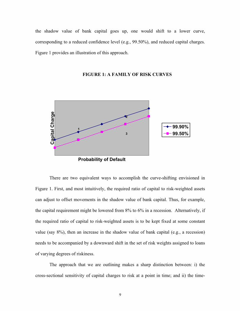
the shadow value of bank capital goes up, one would shift to a lower curve,

corresponding to a reduced confidence level (e.g., 99.50%), and reduced capital charges.

Figure 1 provides an illustration of this approach.

FIGURE 1: A FAMILY OF RISK CURVES

Probability of Default

Cap

ital C

harg

e

99.90%99.50%

1

2

3

There are two equivalent ways to accomplish the curve-shifting envisioned in

Figure 1. First, and most intuitively, the required ratio of capital to risk-weighted assets

can adjust to offset movements in the shadow value of bank capital. Thus, for example,

the capital requirement might be lowered from 8% to 6% in a recession. Alternatively, if

the required ratio of capital to risk-weighted assets is to be kept fixed at some constant

value (say 8%), then an increase in the shadow value of bank capital (e.g., a recession)

needs to be accompanied by a downward shift in the set of risk weights assigned to loans

of varying degrees of riskiness.

The approach that we are outlining makes a sharp distinction between: i) the

cross-sectional sensitivity of capital charges to risk at a point in time; and ii) the time-

10

series sensitivity of capital charges to risk over the business cycle. Consider first the

cross-sectional question. For a fixed point in time, suppose we compare the optimal

capital charges for two different types of loans. This corresponds to moving along a

single curve in Figure 1, say from Point 1 to Point 2. Thus the relative capital charges

for the two types of loans should depend only on their relative riskiness. Or said

differently, capital charges should be fully sensitive to risk in the cross-section.

Now consider the business-cycle question. Suppose we have a fixed loan type,

whose risk increases as we move from an expansionary environment to a recession (think

of a borrower who has been downgraded). This corresponds to a movement across the

two risk curves in Figure 1, say from Point 1 to Point 3. In this case, the capital charge

does not rise as sharply for a given increase in risk as it does in the cross-sectional case.

D. Limitations of the Basel-II Framework

This analysis highlights the problems inherent in the current Basel-II framework,

which envisions a single once-and-for all risk curve, rather than a family of risk curves.

Basel-II would force the cross-sectional slope of the curve—e.g., the ratio of capital

charges for a AA credit and a BBB credit at a fixed point in time—to be the same as the

time-series slope—e.g., the ratio of capital charges for a AA credit who gets downgraded

to BBB during a recession. As we have framed it, this amounts to trying to solve two

problems with a single instrument.

Of course, one can always do better on the time-series problem, say by flattening

the curve, as is illustrated in Figure 2. And indeed, recent revisions to the Basel-II

11

formulas have moved in the direction of such flattening.6 But with a single curve, this

necessarily comes at the expense of doing worse on the cross-sectional problem: a too-

flat curve distorts banks’ pricing of risk at a given point in time, and is likely to be at

odds with the methods that banks (appropriately) use for their internal decisionmaking..

FIGURE 2: A SINGLE FLAT RISK CURVE vs. A FAMILY OF CURVES

Probability of Default

Cap

ital C

harg

e

99.90%99.50%flat

1

2

3

E. Will Banks Offset Cyclicality By Holding Excess Capital?

One argument that is sometimes made is that banks will naturally tend to offset

any potential cyclicality problems, by holding buffer stocks of excess capital during good

times. In the appendix, we argue that while this argument contains a kernel of truth, it is

fundamentally mistaken. A rational farsighted bank may indeed engage in some buffer-

stocking. But loosely speaking, the buffer stock will be set today so that if things turn out

as expected at some future date, the bank will be no more capital-constrained then than it

6 This is not to say that the motivation for these revisions was necessarily to address the particular time-series problem that we have identified here.

12

is today. Of course, the problem with this is that a recession is, almost by definition, an

outcome that is worse than had been anticipated.7 So the realized shadow value of capital

is still likely to go up significantly in a recession (i.e., there is still likely to be something

of a credit crunch), in which case our previous analysis continues to apply. By way of

analogy, this is exactly like saying that even if an individual holds an optimal level of

precautionary savings, he will nevertheless see his consumption fall if he is hit with a

sufficiently adverse unexpected shock—e.g. a serious illness, long-term layoff, etc.

There is a simple reason why a family of risk curves is still preferred to a single

once-and-for-all risk curve, even when banks are farsighted and hold optimal buffer

stocks. When a bank chooses how much capital to hold at some initial point in time, it

cannot know exactly what the shadow value of bank capital will be in the future. In

contrast, with a family of risk curves, the regulator effectively gets to pick the right curve

after the fact, once this shadow value is known.

III. Simulating the Cyclicality of Risk-Based Capital Requirements

A. Overview

We now turn to our empirical analysis. As noted in the Introduction, our aim here

is to simulate the effects that the Basel-II framework could potentially have on the

cyclicality of bank capital requirements. To do so, we study the period from December

1998 to December 2002, an interval that was marked by pronounced economic

slowdowns in both the U.S. and Europe. We also consider three different types of models

7 A similar argument can be made with respect to loan-loss provisions, which can be thought of as an attempt to set aside reserves to deal with expected losses.

13

that banks might conceivably use to estimate PDs under the new rules: i) a model based

on S&P counterparty ratings; ii) a model—due to KMV—that implements a Merton

(1974) approach to estimating default probabilities; and iii) Deutsche Bank’s internal

credit-rating model. In each case, once we have the model-based PD for a given

borrower, we apply “typical” values for the other three parameters (LGD, EAD, and M),

and crank all four of these numbers through the Basel committee’s formula to arrive at

the required capital charge for that borrower.8 In other words, irrespective of the model,

we always apply the same mapping to get from a borrower’s PD to its capital charge.

Wherever possible, we also disaggregate our universe of borrowers along two

dimensions: i) regional (e.g., North America vs. Europe); and ii) credit quality (i.e.,

investment-grade vs. non-investment grade). We do so to get an idea of how the degree

of cyclicality might plausibly vary across banks with different loan portfolios.

B. Methodological Issues

In all of our simulations, the basic goal is to ask how the capital requirements for

a fixed loan portfolio might evolve over the course of a business-cycle downturn. This is

to be contrasted with the question of how an actively-managed portfolio might behave.

In the latter case, active management muddles together the direct effect of a tightened

8 We set LGD = 0.45; M = 2.5 years; and EAD = 1. In all cases, we use the formula for firms in the largest size class by revenues. Note that by keeping LGD fixed over the business cycle, we may be ignoring a source of variability in capital charges, since in reality, it is likely that recovery rates on defaulted loans are lower in recessions. If this is so, and if a given bank’s internal model takes this variation in LGD into account, it will tend to have more cyclicality in (IRB Advanced) capital charges than our results suggest.

14

capital constraint with the bank’s endogenous response. For example, suppose we look at

the evolution of a bank’s actively-managed portfolio during a recession, and find that

average credit quality (and hence the mean capital charge) is roughly unchanged. Should

we conclude from this that there is no cyclicality problem deserving of policymaker

attention? Probably not—it may just be that the bank has reacted to a tightening capital

constraint by cutting off credit to its riskier borrowers, which is precisely the policy

problem that we are concerned with.

Although the fixed-loan-portfolio question sounds straightforward, answering it

with available data requires us to confront several methodological problems.

1. Survivorship bias

One problem that arises across all variants of our simulations is survivorship bias.

This problem can be illustrated by reference to our S&P sample, which we describe in

more detail shortly. The total number of non-defaulted firms that are present in this

dataset as of December 1998 is 3,599. However, even holding aside firms that eventually

default, another 542 of these original firms—about 15%—simply disappear from the

sample by December 2002. These disappearances could reflect mergers, delistings, or

unrecorded defaults.

If one draws the sample for our simulations by imposing the criterion that we

must have data on a firm for all four years 1998-2002 in order for it to be included, this

will create a potentially severe survivorship bias. In the S&P case, this would mean

excluding the 542 firms that disappeared from the data set, and one suspects that these

firms probably had worse-than-average performance over the period, even if they did not

15

default. Thus excluding them would lead us to understate the degree of cyclicality in

capital charges.

Therefore, in all of our simulations we begin with a sample that includes every

non-defaulted firm present in a given data set in 1998. This is in principle the right way

to address the survivorship-bias issue. Of course it raises another question, which is how

we fill in the missing values for those firms that disappear later on in the period.

2. Filling in missing values for firms that disappear from the sample

Suppose that a given firm is in the S&P data set in 1998, with a rating of A-, and

that it also reappears in 1999, with a rating of BB+. After that, it disappears, so we have

no further information on it for 2000, 2001 or 2002. How should we handle this

observation?

We experiment with two different approaches. The first, which we call

“freezing”, sets the rating (or equivalently, the PD) in all the missing years to the last

observed value. Thus in this example, the firm would be assigned a rating of BB+ for

each year in the 2000-2002 interval. This method is simple enough, but almost certainly

biased towards generating too little cyclicality in our particular sample period. We know

that on average firms were being downgraded over this period, so freezing the missing

observations at stale ratings levels prevents us from capturing this tendency.

An alternative approach, which we call “imputation”, works as follows. If firm i

is last observed in year t, we take all firms in the same geographic region and the same

rating class as firm i that survive until t+1. We then impute to firm i in years t+1 the

average rating (and hence average PD) of these surviving peers. In our previous example,

16

the firm that disappears as a BB+ in 1999 would be attributed a rating in 2000 equal to

the average year-2000 rating of all firms in its region that were also BB+ in 1999. We

then follow an analogous procedure for years t+2, etc.

This imputation approach still has its rough edges, but it gets around the basic

problem of assuming that disappearing firms never would have experienced further

downgrades had they remained in the sample. And as we demonstrate below, it generally

leads to estimates of cyclicality that are greater than those that come out of our “freezing”

method.

3. Handling firms that default

A distinct question has to do with how we handle a firm that remains in the

dataset, but is known to be in default. Here again, we experiment with two different

approaches. In the first, we keep defaulted firms in the simulations in all years. Thus if a

firm defaults in 1999, we keep it in as a defaulted firm (with a PD set to 1) in all

subsequent years. With this approach, we always have exactly the same number of

observations in our simulations in each year—i.e., simply the number of firms that were

not in default and present in the data in 1998, 3,599 in the S&P dataset.

Alternatively, we discard defaulted firms in the year after they default. So if a

firm defaults in 1999, we keep it in for 1999, but throw it out thereafter. In our S&P

dataset, this leads us to reduce the number of observations by 304, to 3,295, as of 2002.

Unlike with the freezing vs. imputation approaches, here it is not obvious to us

that one method is inherently more attractive than another. Rather, we see them as

answering two somewhat different questions. When we keep all the defaults in the

17

sample, this tells us something about the total capital shortfall that a bank would have

faced as a result of deteriorating economic conditions over the period 1998-2002, due to

both loan losses and increased capital charges on remaining non-defaulted loans. Of

course, some of this shortfall would have occurred even under the Basel-I rules, as the

bank would have had to eventually recognize losses on defaulted loans in either case.

When we remove defaulted firms from the sample, this is—loosely speaking—like

asking how much additional (as compared to Basel-I) cyclicality Basel-II creates as a

result of the variation in capital charges that it imposes on firms that are downgraded, but

that remain out of default.

An example may help to illustrate this distinction. Consider a bank with 100 in

loans as of 1998, each with a capital charge of 8%. The bank is thus required to hold 8 in

capital; assume that it just meets this constraint with equality in 1998. By 2002, 10 of the

original loans have defaulted, with losses given default of 45% (i.e., the recovery rate is

55%). The remaining 90 in loans that are still on the books have been downgraded, and

each now has a Basel-II capital charge of 10%. Of course, under Basel-I, the capital

charge on these remaining loans would stay at 8%.

If no further capital is raised, the bank’s total stock of capital in 2002 is 3.5—the

original 8, less 4.5 in loan losses from defaults. Under Basel-II, the capital charge for the

remaining loans in 2002 is 9 (9 = 90x10%). So the bank has a total shortfall relative to

its capital requirement of 5.5 (5.5 = 9 – 3.5). Under Basel-I, the capital charge in 2002 is

7.2 (7.2 = 90x8%), and the bank has a total shortfall of 3.7 (3.7 = 7.2 – 3.5). The extra

shortfall created as a result of switching from Basel-I to Basel-II is thus 1.8.

18

If we do not remove defaulted firms from our sample, our methodology will

generate a total “capital charge” for 2002 of 13.5 under Basel-II (13.5 = 90x10% +

10x45%). So we would say that there has been an increase of 5.5 from the initial 1998

level of 8. That is, this approach captures the entire capital shortfall of 5.5 that arises

under Basel-II, due to both downgrades (1.8 of the shortfall) and defaults (3.7 of the

shortfall). In contrast, if we do remove defaulted firms, we only ever look at the non-

defaulted 90 of loans in both 1998 and 2002. For these loans, the capital requirement

goes up by 1.8, from 7.2 to 9.0. Note that this figure of 1.8 corresponds exactly to the

increase in the shortfall that arises as a result of the move from Basel-I to Basel-II.

To summarize, for each of the sets of simulations that follow, we experiment with

four different methodologies:

Method 1: Keep all firms (including defaults) in the sample at all times, and

freeze any missing firms at their last observed rating/PD.

Method 2: Remove firms in the year after they default, and freeze any missing

firms at their last observed rating/PD.

Method 3: Keep all firms (including defaults) in the sample at all times, and use

the imputation technique to deal with any missing firms.

Method 4: Remove firms in the year after they default, and use the imputation

technique to deal with any missing firms.

19

As discussed above, we think that Methods 3 and 4 probably make more sense

than Methods 1 and 2—even though they are a bit less transparent—because the freezing

approach creates an obvious downward bias that is at least partially resolved by

imputation. Whether one prefers Method 3 to Method 4 depends more on the question at

hand: i.e., total cyclicality vs. extra cyclicality created by Basel-II.9 The Method-4

numbers are of by their nature less dramatic, so if one is looking for a conservative set of

estimates, these are probably the ones to look at first.

C. Results From S&P Counterparty Ratings

As noted above, our S&P universe starts with 3,599 non-defaulted firms for which

we have ratings information as of December 1998. We convert each firm’s rating into a

PD, using a fixed correspondence across all regions and time periods.10 The PD’s in turn

can be mapped into capital charges, using the Basel committee’s formula. We then

compute mean capital charges in each year, dealing with defaulted and missing firms

according to the protocols spelled out in Methods 1-4.

In Table 1, we show the percentage change in capital charges over the 1998-2002

period, both for the full sample and for a variety of sub-samples. (When we split the

9 One might argue that Methods 2 and 4 should remove defaulted firms from the data immediately—rather than in the year after they default—if the goal is to get a sense of the purely incremental effect created by the Basel-II downgrading mechanism. The problem with this approach (as applied to annual data) is that it leads us to ignore any within-year downgrades that occur. For example, suppose a firm is rated BB at year-end 1999, slips to CCC by mid-year 2000, and then defaults right before the end of 2000. If we were to delete this firm from the data after 1999, this would amount to ignoring its final and most significant out-of-default downgrade. 10 The mapping is as follows: AAA corresponds to a PD of 0.01%; AA to 0.03%; A to 0.07%; BBB to 0.23%; BB to 1.07%; B to 4.82%; CCC to 22% and D to 100%.

20

sample into investment-grade and non-investment grade subsamples, this split is made

once and for all based on a firm’s rating as of 1998.) If one looks at the results

corresponding to our preferred Method 4, they tell a reasonably consistent story across

Europe and North America, as well as across investment-grade and non-investment grade

firms: increases in capital charges are generally in the range of 30% to 45% over the

period 1998-2002. The “Rest of World” subsample yields considerably higher increases,

in the 80% range, but one should probably not make too much of this particular finding,

as the sample size here is very small—only 320 borrowers in total.

Not surprisingly, Method 3, which keeps defaulted firms in the sample, generates

substantially higher estimates, with numbers in many cases approaching 100%. Again,

however, these numbers are best thought of not as a measure of the incremental degree of

cyclicality associated with the transition from Basel-I to Basel-II, but rather as a measure

of the total capital shortfall that banks experience in a recession, due to a combination of

downgrades and loan losses.

Although the Method-4 estimates are not huge, they still would appear to be

economically significant. One useful benchmark is that the Method-4 estimates are in

most cases at least 40% of the corresponding Method-3 numbers, and sometimes

(typically with investment-grade borrowers) quite a bit more. This suggests that the

added cyclical pressure on bank capital positions associated with Basel-II is of almost the

same order of magnitude as the pre-existing baseline effect under Basel-I.11 In other

words, to the extent that there have previously been concerns expressed about capital

11 If the ratio of the Method-4 to Method-3 estimate is 40%, this suggests that the extra cyclicality effect due to Basel-II is 67% (40/60) of the pre-existing effect due to Basel-I alone.

21

crunches during recessions, the change from Basel-I to Basel-II might be expected to—

very loosely speaking—almost double the impetus behind these episodes.

The Method-4 estimates are also noteworthy in the context of rating agencies’

stated goal of rating borrowers “through the cycle”. Under this approach, a borrower’s

rating is supposed to be based not on its current likelihood of default per se, but instead

on its probability of default in a fixed hypothetical downside scenario. This is clearly

intended to smooth out ratings over the course of a business cycle. But as we can see in

the table, this smoothing is far from total—there still remains a good deal of cyclicality.

D. Results From KMV Model

Table 2 presents our results from the KMV-model simulations. Before comparing

these results to those in Table 1, it is important to note that the samples are quite

different.12 Our KMV sample starts with a much larger universe of firms (17,253 vs.

3,599) and a larger fraction of these firms are non-investment grade than in the S&P data

(58% vs. 38%). One way this shows up is in the mean initial capital charge in 1998: it is

10.72% for the entire KMV sample, vs. 5.85% for the S&P sample.

These differences imply that it may not be too meaningful to directly compare the

cyclicality estimates for the two full samples; these comparisons will be confounded by

the fact that we are not holding the composition of firms constant. It probably makes a

12 In the KMV data, we are not told explicitly when a firm is in default. So we make the following approximation: we regard a firm as defaulted if the KMV model yields an EDFTM (i.e., an estimated default probability) of 20%, and the firm disappears from the data in the following year. We then apply our various sample-selection protocols as before.

22

bit more sense to compare the investment-grade subsamples, where the compositional

differences are likely to be less of an issue.

When we do so, it appears that the KMV methodology leads to substantially more

cyclicality in capital charges. For example, using Method 4 and focusing on all

investment-grade borrowers, the mean S&P-based change in capital from 1998 to 2002 is

44%, while the corresponding KMV number is 83%. This is consistent with previous

research, which has come to the same basic conclusion. And it also fits with the idea that

the KMV approach is meant to deliver a “point-in-time” estimate of default risk, as

opposed to the smoothed, “over-the-cycle” construct used by the rating agencies.13

Interestingly, however, one does not see the same comparative patterns when

focusing on the entire samples, or on the non-investment-grade subsamples. Indeed, for

all non-investment-grade borrowers, the mean KMV-based change in the capital charge

under Method 4 is only 3%. While this may at first seem counter-intuitive, there is in

fact a simple explanation. The initial 1998 capital charge for this non-investment-grade

subsample in the KMV data is so high—at 15.64%—that, if we exclude firms that go into

default, there is just not much room for the remaining non-defaulted firms to see their

capital charges get much higher. Simply put, if one looks at a group of firms that start

out with very low credit ratings, these ratings cannot get much lower outside of default,

and so there can never be more than a modest effect on capital charges as a result of

downgrades.

Conversely, highly-rated firms have much further to fall (again, outside of

default), and so the banks that lend to them are potentially more vulnerable to the sort of

13 A paper published by KMV (“Uses and Abuses of Bank Default Rates,” March 1998) shows that their ratings are in fact considerably more volatile on a year-to-year basis than those from S&P.

23

cyclicality in capital charges induced by the Basel-II framework. This observation brings

us back to our earlier point, about the importance of heterogeneity across banks. Even if

the Basel-II capital requirements do not create a large amount of cyclical variation for all

banks, they may well have large cyclical effects on banks with particular kinds of

portfolios, in this case, banks that lend to relatively high-credit-quality firms.

E. Results From Deutsche Bank Internal Credit Ratings

For our third set of simulations, we use Deutsche Bank’s internal credit-ratings

data. One nice feature of this dataset is that we have information on the size of the (limit)

exposure to individual borrowers, so we can track movements in value-weighted—as

opposed to equal-weighted—capital charges. To the extent that bank portfolios are

unevenly distributed across different types of borrowers, value weighting should present

a more accurate picture of aggregate cyclical effects.

On the other hand, the Deutsche-Bank data also have a couple of drawbacks for

our purposes. First, all the loans are to German firms. This means that the sample may

be less representative of the typical experience in other countries, and also makes

comparison with the S&P and KMV results difficult. Second, there is a much greater

degree of attrition in this dataset. Even setting aside firms that we know have defaulted,

by 2002 we do not have ratings information for over 30% of the initial 1998 sample.

(Recall that the comparable number for the S&P dataset is 15%.) Moreover, the selective

nature of active credit-risk management makes the biases associated with attrition

especially problematic in this case. If firms are dropped in anticipation of future

downgrades, the actual downgrades may never show up in the data, and neither the

24

freezing nor imputation approaches are likely to do much to mitigate this bias.

Consequently, these data may generate misleadingly low estimates of the degree of

capital-charge cyclicality that prevails in the underlying population.

With these caveats in mind, Table 3 presents our results for the Deutsche-Bank

data. The format is similar to that of Tables 1 and 2, with a couple of exceptions. First,

for confidentiality reasons, we are not able to display the initial 1998 capital charges.

Second, we also suppress the Method-1 and Method-2 estimates, since in this case they

turn out to be almost identical to those generated by Methods 3 and 4 respectively.

As can be seen, for the sample of all German firms, Method 4 suggests a

relatively modest increase in the weighted capital charge of 12.65%. For investment-

grade firms, the increase is larger, at 29.78%, and more in line with the estimates coming

from the S&P sample. However, for non-investment-grade firms, there is only a tiny

cyclicality effect of 3.87%, much like what we find for non-investment-grade firms in the

KMV sample.

IV. Related Literature

A handful of other recent papers have attempted to perform simulations more or

less like those in the previous section. These include Carling, Jacobson, Linde and

Roszbach (2002), Catarineu-Rabell, Jackson and Tsomocos (2003), Corcostegui,

Gonzalez-Mosquera, Marcelo and Trucharte (2002), Heid, (2003), Jordan, Peek and

Rosengren (2003), Rosch, (2002), and Segoviano and Lowe (2002). It is hard to directly

compare the numbers across all the studies, because they vary along a number of

dimensions. These include: i) the sample period; ii) the universe of firms under

25

consideration; iii) the model used to derive PD’s; and iv) the fact that different papers use

different iterations of the Basel-committee formula that maps the PD and other credit-risk

parameters into a capital charge. (Recall that this formula has been updated more than

once, most recently in October 2002.)

In Table 4, we take a rough cut at summarizing the key assumptions and results

of several of these other papers; in some cases we have had to read a bit between the lines

to do so. Here we will focus on a couple that seem closest to what we have done:

Catarineu-Rabell, Jackson and Tsomocos (2003), hereafter CJT, and Jordan, Peek and

Rosengren (2003), hereafter JPR. As we do, these papers perform simulations using both

credit ratings and a KMV-based approach.

With respect to the former methodology, CJT examine a sample of Moody’s-rated

firms over the 1990-1992, and estimate an increase in Basel-II capital charges of between

15% and 18% for this period, depending on the sample of firms considered. These

numbers are somewhat lower than the 30%-45% range that we obtained with the S&P

data, using our preferred Method 4. Some of this difference may well be due to the

different sample period, and to the different universe of firms that they consider. But we

speculate that some of it is also likely to be due to CJT not handling survivorship bias in

the same way as us; as best as we can tell, they only consider firms for which data was

available in every year 1990-1992, which raises the sorts of problems discussed above.

One clue that survivorship bias may in fact help to reconcile these results is that

our Method 2, which uses the freezing (rather than imputation) approach to missing

firms—and which, as a result, can be thought of as only a partial fix for survivorship

bias—yields an estimate of 23% for the sample of all firms, quite close to the CJT

26

numbers. Going further, if we totally disregard survivorship issues altogether, and

simply draw our sample from all firms that were present in the S&P database throughout

the period 1998-2002, our estimate falls to 20%.

An essentially identical set of observations apply to JPR. Using S&P credit-rating

data from 1996-2001, they estimate an increase in capital charges of about 20%. This is

closely in line with the results of CJT, and again, somewhat lower than the numbers we

obtain. As with CJT, we suspect that JPR do not take account of survivorship bias in the

same way as we do, and that this helps to explain the why their estimates of cyclicality

are smaller than ours.

With respect to the KMV-based analyses, the qualitative conclusions of CJT run

closely parallel to ours. In particular, they find that the KMV model can induce a much

greater degree of cyclicality in capital charges (they get numbers on the order of 50%,

even without addressing survivorship-bias issues), but that this tends to happen only

when looks at a portfolio of high-credit-quality firms. For firms of lower credit-quality,

the cyclical effects generated by KMV appear to be much more modest in their

simulations, as in ours.14

V. Conclusions

We take two broad messages away from the work reported here. On the empirical

front, our simulations suggest that the new Basel-II capital requirements have the

potential to create an amount of additional cyclicality in capital charges that is, at a

minimum, economically significant, and that may be—depending on a bank’s customer

14 Further confirming evidence on this point comes from Purhonen (2002).

27

mix and the credit-risk models that it uses—quite large. Our empirical analysis also

underscores the importance of dealing with various methodological issues that crop up in

this context, most notably survivorship bias. As we have shown, failure to do so can lead

to estimates of cyclicality that are substantially downward-biased.

On the theory side, our main point has been that the Basel-II approach of having a

single time-invariant risk curve is, in principle, sub-optimal. Instead, it is more desirable

to have a family of risk curves—i.e., to tolerate a greater probability of default when

economy-wide bank capital is scarce relative to lending opportunities.

One possible objection to this conclusion is that it is naïve with respect to

political-economy considerations. In particular, one might argue that any theory that

suggests reducing capital requirements in bad times will simply give regulators an excuse

to engage in after-the-fact forbearance, with all the accompanying potential for various

forms of regulatory moral hazard.

While we agree that such moral hazard concerns are of great importance, we

believe the above argument can be turned on its head. If it really is the case that capital

requirements need to come down, say, in a severe recession, it is probably better to

acknowledge this fact of life up front, and to explicitly codify the magnitude of the

adjustment. Such ex ante codification will, if anything, tend to reduce regulators’ ex post

discretion, thereby tempering moral hazard problems. In contrast, with an unrealistically

rigid ex ante rule that never contemplates the need to reduce capital requirements, the risk

is that in a sufficiently bad scenario, the rule will become de facto untenable. At this

point, it will be left to regulators to relax the rule as they see fit—perhaps on a highly

corruptible case-by-case basis—without any previously-imposed constraints.

28

Of course, this discussion raises the question of how one designs a credible,

transparent formula that links capital requirements to some measure of aggregate

economic conditions. This is a difficult question, and not one that we are prepared to

answer fully. But we can venture a few tentative thoughts. At one extreme, it is easy to

imagine crude rules that are based on aggregate business-cycle indicators. For example,

one might drop the required ratio of capital to risk-weighted assets from 8% to 6%

whenever GDP growth falls below some threshold.15

While formulas of this sort seem like they would be easy enough to implement,

there may be a good deal of slippage between something like GDP growth and the

construct that the theory tells us should be relevant, namely the shadow value of bank

capital. Alternatively, one can try to come up with other, more sophisticated indicators

that track this shadow value more closely.16 The tradeoff is that an overly complicated,

hard-to-verify measure is probably not much better than no measure at all.

One trick that might get around these problems would be to create a market for

regulatory capital relief. In particular, suppose that the regulator periodically auctions off

a small supply of tradable certificates, each of which entitles the holder to breach the

standard 8% capital requirement by, e.g., $1 million for one year. The market price of

these certificates would then be a direct and transparent measure of the shadow value of

bank capital—i.e., a high price would indicate a relative shortage of bank capital.

15 Here we are also ignoring all the problems associated with the timing of data releases and the revisions to macro data. 16 For example, following Kashyap, Stein and Wilcox (1993), one might look at the ratio of commercial-paper issuance to bank-loan growth as a measure of tightness in bank loan supply, and hence as a proxy for the relative scarcity of bank capital. But doing this kind of indexation properly will likely require a number of adjustments to account for trends in the data, other sources of shocks, etc.

29

Moreover, by allowing the regulator to increase the supply of certificates in the face of

rising prices, it would become possible to tie the effective capital requirement to this

shadow value, just as the theory suggests should be done.

We should stress that this last suggestion is intended in the spirit of preliminary

brainstorming, and nothing more; we have not even begun to come to grips with the

many practical complexities that it would surely entail. However, our aim here is not to

push any one particular proposal for linking capital requirements to economic conditions.

Rather, we just hope to call attention to the general issue, and to illustrate that there is a

lot of room for further thought with respect to it.

30

Appendix: A Model of Optimal Capital Requirements

A. The Unregulated Bank’s Objective Function

Consider a bank that at any point in time t can invest in n different types of loans,

with the investment in each type denoted by L1t……… Lnt. The expected net return on

loan type i at time t is given by: θtfi(Lit) – (1 + rit)Lit, where fi( ) is a concave function, θt

is an indicator of the state of the economy at time t, and rit is the bank’s risk-adjusted

discount rate for category i at time t. The concavity of fi( ) captures the idea that the more

loans a bank makes in a given category, the lower will be the rate it can charge on the

marginal loan.

Let us first ask what happens in the absence of any capital regulation. At any

time t, the bank faces the following static optimization problem:

Max θt Σ fi(Lit) – (1 + rit)Lit (1)

For any loan category i, this implies the following first-order condition:

θt f′i(Lit) = (1 + rit) (2)

This condition just says that the bank equates the marginal return on each loan type to the

appropriate discount rate.

B. The Social Planner’s Objective Function

In order to introduce a rationale for capital regulation, we need to assume that

bank default has social costs that are not internalized by the bank itself. Let the added

31

social cost of bank default be given by X. Suppose further that the bank has a stock of

capital Kt at time t, and that, for simplicity, it cannot adjust its capital.17 The probability

that the bank will default at any point in time, which we denote by πt, depends on both

the nature of its loan portfolio, and how much capital it is holding. Without specifying

the functional form, we can write: πt = πt(L1t……… Lnt; Kt).

Suppose that the social planner’s objective function resembles the bank’s, with

the one modification being that the social planner internalizes the extra default cost X.

The social planner’s problem at time t can therefore be written as:

Max θt Σ fi(Lit) – (1 + rit)Lit – Xπt(L1t……… Lnt; Kt) (3)

For any loan category i, this implies the following first-order condition:

θt f′i(Lit) = (1 + rit) + Xdπt/dLit (4)

Here dπt/dLit is the marginal contribution of loan type i to overall default risk at time t.

Under certain restrictive conditions, dπt/dLit will be a function only of the

attributes of loan type i—such as its probability of default (PD) and its loss given default

(LGD)—and will be independent of the rest of the bank’s loan portfolio.18 In this case,

optimally-designed capital requirements at any point in time will resemble those being

17 Extending the model to the case where capital can be adjusted at some cost—reflecting, e.g., adverse-selection frictions in the market for new equity issues—yields similar results. 18 See Gordy (2003). Loosely speaking, the conditions required are that asset returns are generated by a single-factor process, and that a bank’s exposure to any single loan type is infinitesimally small.

32

considered under the Basel-II accord. But as stated, (4) applies irrespective of whether

these restrictive conditions hold—it is only a general statement of the fact that social

optimality requires the marginal return on each loan type to be equal to the bank’s

discount rate, plus the marginal contribution of that loan type to social default costs.

A key observation about (4) is that while the social planner cares about bank

default risk, he does not care about it to the exclusion of all other considerations. In

particular, the social planner naturally also puts some weight on the efficiency of bank

lending. This suggests that if bank capital were particularly scarce at a given point in

time, the social planner would be willing to tolerate a higher probability of bank default,

in order to partially insulate lending—i.e., in order not to drive the marginal return on

bank loans too far above the appropriate discount rate.

C. Implementing the Social Optimum With Risk-Based Capital Requirements

While (4) describes the optimum from the social planner’s perspective, it does not

say how this optimum is implemented with capital regulation. To address this issue, note

that a general formulation of risk-based capital requirements imposes the following

constraint on the bank at time t:

Σ atwitLit ≤ Kt (5)

where at is the required ratio of capital to risk-weighted assets at time t (e.g., 8%, as

envisioned in the Basel-II framework), and where wit is the risk weight applied to loan

category i at time t. The product atwit is then the total capital charge per dollar for loan

type i at time t.

33

Suppose that the regulator imposes a capital requirement of this form on a bank,

and that the bank is then free to optimize its portfolio, subject to satisfying the capital

requirement. In other words, the bank’s objective function is still given by (1), but now

subject to the constraint in (5). The bank’s first-order condition for any loan category i

can be written as:

θt f′i(Lit) = (1 + rit) + λtatwit (6)

where λt is the shadow value of bank capital at time t. Simply put, the bank’s investment

in any given loan type is cut back by an amount that reflects the bank’s overall scarcity of

capital (i.e., λt), and by the amount of capital that the loan type requires (i.e., atwit). The

shadow value of capital is itself given by:

λt = [θt f′k(Lkt) – (1 + rkt)]/atwkt (7)

for any k. In other words, the shadow value of capital reflects the extent to which the

bank is underinvesting in lending activity, relative to the case in which it is not

constrained by capital regulation.

It should now be clear how a regulator can use capital requirements to implement

the social optimum. The social optimum is given by (4). For any arbitrary set of capital

requirements, the bank’s induced behavior is given by (6). Setting the two expressions

equal to one another yields the capital requirements that make the bank behave as the

social planner would like. These can be written as:

34

atwit = (X/λt)dπt/dLit (8)

where atwit is the amount of capital that must be held against one dollar of a loan of type

i at time t.

Observe that this capital requirement is not only a function of the loan’s

contribution to expected default costs, Xdπt/dLit. Rather, when the overall shadow value

of bank capital λt is higher, socially optimal regulation requires that the capital

requirement be reduced, all else equal. The intuition is straightforward: the regulator

should trade off default risk against the costs associated with underinvestment in bank

loans. When the shadow value of bank capital is higher—i.e., when bank capital is

scarcer relative to positive-NPV lending opportunities, the underinvestment problem is

worse, so there should be a greater willingness to tolerate default risk.

This analysis highlights the crucial distinction between: i) the cross-sectional

sensitivity of capital requirements to risk at a point in time; and ii) the time-series

sensitivity of capital requirements to risk over the business cycle. Consider first the

cross-sectional question. For a fixed point in time t, suppose we compare the optimal risk

weights for two loans of types i and j, respectively. From (8), it follows that:

wit/wjt = (dπt/dLit)/(dπt/dLjt) (9)

Thus the relative risk weights for the two types of loans depend only on their

relative riskiness, i.e., their relative contributions to the probability that the bank will

35

default. Or said differently, risk weights should be fully sensitive to risk in the cross-

section. Thus if we plot the optimal risk weights (or equivalently, capital charges) as a

function of a risk measure—say the PD—at a given point in time, this “risk curve” ought

to be steeply upwards sloping, as illustrated in Figure 1 in the text.

Things are more complicated if we look at the evolution of the capital

requirement for a given loan type i across two different points in time, T and t. Now (8)

tells us that:

atwit/aTwiT = λT(dπt/dLit)/λt(dπT/dLiT) (10)

For concreteness, think of time T as being during a business-cycle expansion, and

time t as being in a period of recession. It is likely that the riskiness of loan i will

increase in a recession, so that (dπt/dLit) > (dπT/dLiT). But according to (10), the relative

capital charge need not go up one-for-one with this increase in risk, if the shadow value

of bank capital rises in a recession—i.e., if λt > λT.

From (10), it is clear that there are two equivalent ways to accomplish the desired

intertemporal smoothing of capital charges. First, and most intuitively, the risk weights

can continue to be fully risk-sensitive over time as well as in the cross-section, and the

required ratio of capital to risk-weighted assets can adjust to offset movements in the

shadow value of bank capital. This corresponds to having wit/wiT = (dπt/dLit)/(dπT/dLiT);

and at/aT = λT/λt. Alternatively, if the required ratio of capital to risk-weighted assets a

is to be kept fixed at some constant value (say 8%), then an increase in the shadow value

of bank capital (e.g., a recession) needs to be accompanied by a downward shift in the set

36

of risk weights. This corresponds to having wit/wiT = λT(dπt/dLit)/λt(dπT/dLiT). Either

approach amounts to tolerating a higher probability of bank default when the shadow

value of bank capital goes up. Equivalently, either approach can be thought of as a

downward shift in the “risk curve” that relates capital charges to measures of riskiness

such as the PD. Thus optimality requires a family of point-in-time risk curves, with each

curve corresponding to a different shadow value of bank capital—i.e., to different

macroeconomic conditions. This is the approach illustrated in Figure 1 in the text.

D. Limitations of the Basel-II Framework

This discussion makes clear the problems inherent in the current Basel-II

framework, which envisions a single once-and-for all risk curve, rather than a family of

risk curves. Basel-II would force the cross-sectional slope of the curve—e.g., the ratio

of capital charges for a AA credit and a BBB credit at a fixed point in time—to be the

same as the time-series slope—e.g., the ratio of capital charges for a AA credit who gets

downgraded to BBB during a recession. This amounts to trying to solve two problems

with a single instrument.

Of course, one can always do better on the time-series problem, say by flattening

the curve, as is illustrated in Figure 2. And indeed, recent revisions to the Basel-II

formulas have moved in the direction of such flattening. But with a single curve, this

necessarily comes at the expense of doing worse on the cross-sectional problem: a too-

flat curve distorts banks’ pricing of risk at a given point in time.

37

E. Will Banks Eliminate the Problem By Holding Excess Capital?

One argument that is sometimes made is that banks will naturally tend to offset

any potential problems associated with time-varying capital charges, by holding buffer

stocks of excess capital during good times. In the context of the above model, this

amounts to saying that dynamic optimization on the part of banks will force the shadow

value of capital to be equalized at all points in time. Thus, for example, in equation (10),

we would have λt = λT for any two dates t and T, and the whole family of risk curves

discussed above can be collapsed to a single risk curve.

Although this argument has a kernel of truth to it, it is fundamentally mistaken.

Without developing a full-blown dynamic model, we note that intertemporal optimization

by a farsighted bank can at best tend to equate the shadow value of capital today to the

expected shadow value at some future date. In other words, if time T precedes time t, we

would not have λt = λT, but rather λT = ET (λt ), where ET ( ) denotes the expectation as of

time T.

Thus if T is a time of business-cycle expansion, the bank may indeed hold a buffer

stock of excess capital. But loosely speaking, this buffer stock will be set so that if things

turn out as expected at the future date t, the bank will be no more capital-constrained at t

than it was at T. Of course, the problem with this is that a recession is, almost by

definition, an outcome that is worse than had been anticipated. So the realized shadow

value of capital is still likely to go up significantly in a recession, in which case our

previous analysis continues to apply. By way of analogy, this is exactly like saying that

even if an individual holds an optimal level of precautionary savings, he will nevertheless

38

see his consumption fall if he is hit with a sufficiently adverse unexpected shock—e.g. a

serious illness, long-term layoff, etc.

There is a simple reason why a family of risk curves is still preferred to a single

once-and-for all risk curve, even when banks are farsighted and hold optimal buffer

stocks. When a bank chooses how much capital to hold at some initial time T, it cannot

know exactly what the shadow value of bank capital will be when time t arrives. In

contrast, with a family of risk curves, the regulator effectively gets to pick the right curve

after the fact, once this shadow value is known.

39

References

Basel Committee on Banking Supervision (2003), “Overview of the New Basel Capital Accord,” BIS consultative document.

Bernanke, Ben (1983), “Nonmonetary Effects of the Financial Crisis in

Propogation of the Great Depression,” American Economic Review 73: 257-276. Bernanke, Ben and Carla Lown (1991), “The Credit Crunch,” Brookings Papers

on Economic Activity: 204-239. Carling, Kenneth, Tor Jacobson, Jesper Linde and Kasper Roszbach (2002),

“Capital Charges under Basel II: Corporate Credit Risk Modeling and the Macroeconomy,” Sveriges Risksbank working paper 142.

Catarineu-Rabell, Eva, Patricia Jackson and Dimitrios Tsomocos (2003),

“Procyclicality and the New Basel Accord—Banks’ Choice of Loan Rating System,” Bank of England working paper 181.

Corcostegui, Carlos, Luis Gonzalez-Mosquera, Antonio Marcelo and Carlos

Trucharte (2002), “Analysis of Procyclical Effects on Capital Requirements Derived From a Rating System,” working paper.

Cosandey, David and Urs Wolf (2002), “Avoiding Pro-cyclicality,” RISK,

October: S20-S21. Ervin, D.W. and T. Wilde (2001), “Pro-cyclicality in the New Basel Accord,”

RISK, October. Gordy, Michael B. (2003), “A Risk-Factor Model Foundation for Ratings-Based

Bank Capital Rules,” Journal of Financial Intermediation 12: 199-232. Heid, Frank (2003), “Is Regulatory Capital Pro-cyclical? A Macroeconomic

Assessment of Basel II,” Deutsche Bundesbank working paper. Jackson, Patricia (2002), “Bank Capital: Basel II Developments,” Financial

Stability Review, December: 103-109. Jordan, John, Joe Peek and Eric Rosengren (2003), “Credit Risk Modeling and the

Cyclicality of Capital,” working paper. Kashyap, Anil K, Jeremy C. Stein and David Wilcox (1993), “Monetary Policy

and Credit Conditions: Evidence from the Composition of External Finance,” American Economic Review, 83: 78-98.

40

Lowe, Philip (2002), “Credit Risk Measurement and Procyclicality,” BIS working paper 116. Merton, Robert (1974), “On the Pricing of Corporate Debt: The Risk Structure of Interest Rates,” Journal of Finance 29: 449-470. Peek, Joe, and Eric Rosengren (1995), “The Capital Crunch: Neither a Borrower Nor a Lender Be,” Journal of Money, Credit and Banking 27: 625-638. Peek, Joe and Eric Rosengren (1997), “The International Transmission of Financial Shocks: The Case of Japan,” American Economic Review 87: 495-505. Purhonen, Martti (2002), “New Evidence of IRB Volatility,” RISK, March: S21-S25. Rosch, Daniel (2002), “Mitigating Procyclicality in Basel II: A Value at Risk Based Remedy,” working paper, University of Regensburg. Segoviano, Miguel and Philip Lowe (2002), “Internal Ratings, the Business Cycle and Capital Requirements: Some Evidence From An Emerging Market Economy,” BIS working paper 117.

41

Table 1: Capital-Charge Cyclicality, 1998-2002, Using S&P Ratings

Method Region Rating Class

Initial Capital, 1998

%Change Capital, 98-02 Method Region

Rating Class

Initial Capital, 1998

%Change Capital, 98-02

1 All All 5.85 78.00 3 All All 5.85 86.361 All IG 2.40 56.38 3 All IG 2.40 59.281 All non-IG 11.59 85.44 3 All non-IG 11.59 95.661 Europe All 3.05 54.53 3 Europe All 3.05 66.211 Europe IG 1.84 39.61 3 Europe IG 1.84 41.491 Europe non-IG 12.19 71.69 3 Europe non-IG 12.19 94.651 North America All 6.28 77.03 3 North America All 6.28 84.361 North America IG 2.52 54.04 3 North America IG 2.52 56.921 North America non-IG 11.56 84.04 3 North America non-IG 11.56 92.731 Rest of World All 6.07 103.71 3 Rest of World All 6.07 118.991 Rest of World IG 2.55 100.56 3 Rest of World IG 2.55 105.101 Rest of World non-IG 11.70 104.81 3 Rest of World non-IG 11.70 123.842 All All 5.85 22.72 4 All All 5.85 31.452 All IG 2.40 40.75 4 All IG 2.40 43.672 All non-IG 11.59 30.42 4 All non-IG 11.59 42.902 Europe All 3.05 21.44 4 Europe All 3.05 33.402 Europe IG 1.84 39.61 4 Europe IG 1.84 41.492 Europe non-IG 12.19 18.90 4 Europe non-IG 12.19 47.862 North America All 6.28 18.69 4 North America All 6.28 26.812 North America IG 2.52 34.73 4 North America IG 2.52 37.642 North America non-IG 11.56 26.59 4 North America non-IG 11.56 37.662 Rest of World All 6.07 65.35 4 Rest of World All 6.07 77.892 Rest of World IG 2.55 92.48 4 Rest of World IG 2.55 97.042 Rest of World non-IG 11.70 69.09 4 Rest of World non-IG 11.70 87.92

Notes to Table 1: IG refers to all firms with a rating of BBB- or better in December 1998; non-IG refers to those with a rating of BB+ or worse. There are 3,599 observations in the full sample (2,247 IG and 1352 non-IG); 456 in the Europe subsample (403 IG and 53 non-IG); 2,823 in the North America subsample (1647 IG and 1176 non-IG); and 320 in the Rest-of-World subsample (197 IG and 123 non-IG).

42

Table 2: Capital-Charge Cyclicality, 1998-2002, Using KMV Model

Method Region Rating Class

Initial Capital, 1998

%Change Capital, 98-02 Method Region

Rating Class

Initial Capital, 1998

%Change Capital, 98-02

1 All All 10.72 33.31 3 All All 10.72 35.91 1 All IG 4.01 101.43 3 All IG 4.01 111.47 1 All Non-IG 15.64 20.54 3 All non-IG 15.64 21.61 1 Germany All 5.78 82.24 3 Germany All 5.78 82.24 1 Germany IG 3.40 161.91 3 Germany IG 3.40 161.91 1 Germany Non-IG 12.16 24.56 3 Germany Non-IG 12.16 24.56 1 Rest of Eur. All 7.26 56.04 3 Rest of Eur. All 7.26 62.53 1 Rest of Eur. IG 3.66 123.56 3 Rest of Eur. IG 3.66 139.07 1 Rest of Eur. Non-IG 13.12 25.28 3 Rest of Eur. non-IG 13.12 27.90 1 North America All 12.17 41.70 3 North America All 12.17 44.45 1 North America IG 4.34 95.62 3 North America IG 4.34 107.60 1 North America Non-IG 16.56 33.79 3 North America non-IG 16.56 35.14 1 Rest of World All 11.81 10.50 3 Rest of World All 11.81 11.09 1 Rest of World IG 4.12 75.39 3 Rest of World IG 4.12 77.91 1 Rest of World Non-IG 15.69 1.90 3 Rest of World non-IG 15.69 2.17

2 All All 10.72 11.54 4 All All 10.72 13.81 2 All IG 4.01 75.02 4 All IG 4.01 82.54 2 All Non-IG 15.64 2.06 4 All non-IG 15.64 3.20 2 Germany All 5.78 59.11 4 Germany All 5.78 59.11 2 Germany IG 3.40 113.57 4 Germany IG 3.40 113.57 2 Germany Non-IG 12.16 18.50 4 Germany Non-IG 12.16 18.50 2 Rest of Eur. All 7.26 25.68 4 Rest of Eur. All 7.26 31.27 2 Rest of Eur. IG 3.66 80.79 4 Rest of Eur. IG 3.66 92.62 2 Rest of Eur. Non-IG 13.12 2.80 4 Rest of Eur. non-IG 13.12 5.64 2 North America All 12.17 7.34 4 North America All 12.17 9.86 2 North America IG 4.34 64.17 4 North America IG 4.34 73.27 2 North America Non-IG 16.56 2.74 4 North America non-IG 16.56 4.23 2 Rest of World All 11.81 9.90 4 Rest of World All 11.81 10.33 2 Rest of World IG 4.12 78.61 4 Rest of World IG 4.12 80.34 2 Rest of World Non-IG 15.69 1.44 4 Rest of World non-IG 15.69 1.72

Notes to Table 2: IG refers to all firms with a KMV EDFTM of 0.94% or better in December 1998; non-IG refers to the remainder. (This breakpoint is obtained by calculating the mean values of EDFTM for BBB-rated and BB-rated firms, and then taking the midpoint.) There are 17,253 observations in the full sample (7,292 IG and 9,961 non-IG); 378 in the Germany subsample (275 IG and 103 non-IG); 4,183 in the Rest-of-Europe subsample (2,593 IG and 1,590 non-IG); 7,051 in the North America subsample (2,532 IG and 4,519 non-IG); and 5,641 in the Rest-of-World subsample (1,892 IG and 3,749 non-IG).

43

Table 3: Capital-Charge Cyclicality, 1998-2002, Using Deutsche Bank Internal Data

Method Region Rating Class %Change Capital, 98-02

3 Germany All 26.65 3 Germany IG 37.28 3 Germany non-IG 32.12

4 Germany All 12.65 4 Germany IG 29.78 4 Germany non-IG 3.87

Notes to Table 3: Unlike in Tables 1 and 2, observations are weighted by the limit size of the exposure. IG refers to all firms with an internally-estimated PD of 0.5% or better in December 1998; non-IG refers to the remainder. There are 56,941 observations in the full sample (27,052 IG, and 29,889 non-IG).

44

Table 4: Summary of Other Research on Capital-Charge Cyclicality

Study Country Time Period

Capital Charge Basis

Max Change in Capital

Notes

Ervin and Wilde (2001)

U.S. 1990-1992

? 20% All BBB borrowers

Foundations, 11/01

69.8% Segoviano and Lowe (2002)

Mexico (Customers of main large banks)

3/1995- 12/1999 Standardized 57.1%

Includes E rated loans, peak losses are in 12/96 Capital changes inferred from their Table 2

Foundations, 11/01

56.7% Segoviano and Lowe (2002)

Mexico (Customers of main large banks)

3/1995- 12/1999 Standardized 15.7%

Excludes E rated loans, peak losses are in 12/96 Capital changes inferred from their Table 2

U.S. high quality banks’ customers

15.2%

U.S. ave. quality banks’ customers

17.9%

Catarina-Rabell, Jackson, and Tsomocos (2003)

Same quality customers as Deutsche Bank

1990-1992

QIS 3, 10/02

15.3%

Based on Moody’s ratings transitions of 5,022 non-defaulting corporate borrowers, using different initial borrower distributions described in column 2

U.S. high quality banks’ customers

53.2%

U.S. ave. quality banks’ customers

8.8%

Catarina-Rabell, Jackson, and Tsomocos (2003)

Same quality customers as Deutsche Bank

1990-1992

QIS 3, 10/02

47.1%

Based on Merton model PD transitions of 282 borrowers, using different initial borrower distributions described in column 2

S&P: ≈ 20% Jordan, Peek and Rosengren (2003)

U.S. 1996-2001

11/01 KMV: ≈ 280%

Shared National Credit borrowers, all loans exceed $20 million

Rosch (2002) U.S. 1982-2000

11/01 +15% Multiple 1 year swings of this size, based on S&P transitions

Corcostegui, Gonzalez-Mosquera, Marcelo, and Trucharte (2002)

Spain 1993-2000

QIS 3, 10/02 -6.1 percentage points of capital

No base level given, +3.1 p.p. the year before this swing

-11.23 percentage points of capital

Carling, Jacobson, Lindé, and Roszbach (2002)

Sweden 1994-2000

1/01

-20.37 percentage points of capital

No base level of capital given, two methods of gauging PDs, either historical default experience (top) or based on one bank’s internal model (bottom)