d 2.3 neuronal culture/slice experimental setup and...
TRANSCRIPT

Proposal full title:
INSIGHT: Darwinian Neurodynamics
Proposal acronym:
INSIGHT
Type of funding scheme:
Collaborative project
FP7-ICT-2011-C FET Open
Name of the coordinating person:
Prof. Eörs Szathmáry
Coordinator email: [email protected]
Coordinator phone: +49 89 4520935-30
Coordinator fax: +49 89 4520935-31
D 2.3
Progress of neuronal culture/slice experimental
setup and analysis method
Milestone 4: Development of culture system with electrophysiology/optical methods

INSIGHT
FP7-ICT-2011-C
Project n. 308943
Deliverable No. 2.3 Revision n. 3 Page | 2
Revisions Tables
Due delivered date 28/02/2014 Actual delivered date 21/03/2014
Lead beneficiary UoS
Beneficiaries involved UoS
Authors Kevin Staras, Terri Roberts, James Thorniley, Phil Husbands
Dissemination level PU Nature R
REV Work performed Reviewers Beneficiary
1 Production of the deliverable Phil Husbands UOS
2 Final revision Eörs Szathmary PARMENIDES
3 Formatting Roberta Modolo IN

INSIGHT
FP7-ICT-2011-C
Project n. 308943
Deliverable No. 2.3 Revision n. 3 Page | 3
Table of contents
1 Executive summary ..................................................................................................................................................... 5
2 Technical Considerations ....................................................................................................................................... 5
3 Establishing cultured neurons for MEA work ................................................................................................... 6
3.1 Method ................................................................................................................................................................. 6
3.2 Results ................................................................................................................................................................... 7
4 Developing the MEA recording approach ......................................................................................................... 9
4.1 MEA Setup ............................................................................................................................................................ 9
4.2 Strategy for high data yield in MEA experiments .................................................................................. 9
4.3 Astrocyte-neuron culture in MEA .............................................................................................................. 11
4.4 Activity and stimulation ................................................................................................................................. 13
5 MEA for acute slice recording work ................................................................................................................... 14
6 Software Tools for Analysis ................................................................................................................................... 16
6.1 Overview ............................................................................................................................................................. 16
6.2 Software requirements ................................................................................................................................... 16
6.3 Problem analysis ............................................................................................................................................... 19
6.3.1 Data formats ............................................................................................................................................. 19
6.3.2 Converting raw data with MC_DataTool ........................................................................................ 19
6.3.2 Extracting spikes using MC_Rack, then converting with MC_DataTool.............................. 20
6.3.3 Importing data with the Neuroshare framework ........................................................................ 20
6.3.4 Reading data with the MC_Stream C++ library .......................................................................... 22
6.4 Spike extraction approach ............................................................................................................................ 24
6.5 Implementation overview ............................................................................................................................. 27
6.5.1 System architecture ................................................................................................................................ 27
6.5.2 Framework and platform libraries .................................................................................................... 28
6.5.3 Internal data formats ............................................................................................................................. 29
6.5.4 Processing Pipeline ................................................................................................................................ 29
6.5.5 Kernels ......................................................................................................................................................... 31
6.5.6 Plots ............................................................................................................................................................. 32
6.5.7 NPZ file specification ............................................................................................................................. 33
7 Causal Inference......................................................................................................................................................... 34
7.1 Background information: inferring causation ....................................................................................... 34
7.2 Causality measures .......................................................................................................................................... 36
7.3 Information transfer in embodied agents .............................................................................................. 37
7.4 Causality detectors .......................................................................................................................................... 38
References ............................................................................................................................................................................. 39
Appendix A: Software tools mcd library description ............................................................................................ 42
Appendix B: Software Build Process ............................................................................................................................ 44

INSIGHT
FP7-ICT-2011-C
Project n. 308943
Deliverable No. 2.3 Revision n. 3 Page | 4
Appendix C: Software Tools User Guide .................................................................................................................... 50
Appendix D: Hippocampal Slice Paper ....................................................................................................................... 57

INSIGHT
FP7-ICT-2011-C
Project n. 308943
Deliverable No. 2.3 Revision n. 3 Page | 5
1. Executive summary
The objective of this component of WP2 is to establish an experimental preparation and paradigm
appropriate for investigating spatio-temporal copying of information between two- and three-
neuron groups in physiologically-relevant vertebrate neuronal networks. The aim is to gather
experimental evidence to support theoretical proposals being developed elsewhere in this work
related to Darwinian neurodynamics. This is a challenging task and depends on the development of
a robust preparation for assaying and modulating activity in populations of interconnected neurons
capable of undergoing activity-dependent plasticity. Although this is a first year report, this two-
year experimental component had a delayed start (for reasons beyond our control – delayed
signing of Grant Agreement document) and at the present time has been running for six months.
Nonetheless, as we summarize below, progress has been good and we have met the key twelve
month deliverables and milestone in the work so far (M4: Development of culture system with
electrophysiology/optical methods). Specifically, we have established suitable preparations based
on both primary neuronal cultures and acute brain slice, determined their viability by imaging and
electrophysiological means, constructed a fully-operational multi-electrode array set-up,
established its capability to assay and influence neuronal activity and developed the key software
tools necessary to control experiments and analyze data. Analysis techniques based around the
concept of causality have also been developed as these will be very pertinent to the ‘causal
copying’ experiment to be carried out in the next phase of work. In the next eighteen months we
expect to build on this substantial progress and initiate the training experiments planned for this
work component.
2. Technical Considerations
We set out to first establish a healthy neuronal preparation to use for this work. Possible viable
options include cultured neurons and acute brain slices. Cultured neurons are reconstituted circuits
whose parameters of organization (e.g. density) and activity-dependent history can be relatively
well-specified. However, they exhibit non-physiologically-relevant wiring and require in excess of
three weeks to achieve operational maturity. Acute slices are tissue volumes excised directly from
adolescent rat brain. As such, circuits are natively wired and five or more slices can be used within
hours of preparation. However, they are numerically complex with less-defined activity history and
present technical challenges for readout of population activity. Both therefore have advantages and
disadvantages for this work. The second consideration is the approach for assaying neuronal
activity and implementing plasticity induction profiles. Optical imaging methods allow for excellent
remote reporting of individual neuronal parameters (for example synaptic transmission and single
neuron spike activity) and with optogenetic techniques offer controlled stimulation parameters;
nonetheless, they offer poor solutions for long-term readouts across cell populations. Alternatively,
multi-electrode arrays (MEAs), based on extracellular recording methods, provide a robust solution
INSIGHT
FP7-ICT-2011-C
Project n. 308943
Deliverable No. 2.3 Revision n. 3 Page | 6
for sampling network spiking activity at electrodes - effectively ‘nodes’ representing collective
output of one or several neurons local to an electrode - as well applying targeted stimulation. In
view of these considerations, we selected the following strategy: First, development of cultured
neurons for MEA-work, with parameters of viability and transmission initially confirmed with optical
imaging approaches. Second, once the MEA setup is established, development of an acute brain
slice preparation for use in the same system, offers the opportunity to explore experimental
parameters which might be critically dependent on native high-density cytoarchitecture and wiring.
This report outlines our progress in these objectives.
3. Establishing cultured neurons for MEA work
3.1 Method
Cultures. Dissociated hippocampal cultures are prepared from postnatal day (P)0 rats by plating
neurons onto a poly-d-lysine (PDL) coated substrate, and maintained in basal medium eagle (BME)
media with 45% glucose, 2% fetal calf serum (FCS) and B27/Glutamax supplement. This substrate is
either the bottom of the multi-electrode array or a separate 12 mm coverslip which can be inverted
onto the array (see results). For most experimental approaches, the local environment also included
an astrocyte feeder layer, either pre-plated onto the PDL substrate or onto a second coated
substrate lying parallel to the first (see results for details on preparation development). The cultures
were maintained as described previously (Darcy et al., 2006; Morales et al., 2000) and used for
experiments at 11-30 days in vitro. Animal care and use protocols were approved by the Home
Office (UK) and complied with local institutional regulations. Unless otherwise stated, all
experiments were performed in external bath solution (137 mM NaCl, 5 mM KCl, 2.5 mM CaCl2, 1
mM MgCl2, 10 mM D-Glucose, 5 mM HEPES) at 25 oC or 37oC.
Imaging and MEA set-ups. Fluorescence imaging was carried out with an upright Olympus BX61WI
microscope using a x60 1.0 N.A. dipping objective. Excitation and emission filter sets for
fluorescence imaging were as follows: 480/20 nm, 520/35 nm. For imaging experiments, neurons
were transfected at days in vitro 7-9, using a Ca2+ phosphate protocol. Image analysis was
performed using ImageJ (http://rsb.info.nih.gov/ij/) on raw unfiltered images or after filtering (1×1
median filter) applied to the whole image. Cultures were electrically activated via a field stimuIation
chamber using 20 V 1 ms square waveforms. Brain slice work used an Olympus BX51WI upright
microscope with confocal head (Fluoview FV300) coupled to an Ar laser and Molecular Devices
Multiclamp 700B for recording and stimulation. MEA-based experiments used an inverted Nikon
Optiphot. Details of MEA-setup are outlined in Results below.
Slice preparation. Acute transverse slices of hippocampus (300 μm) were prepared from 3- to 4-
week-old rats and maintained in artificial cerebrospinal fluid (aCSF) containing 125 mM NaCl, 2.5
mM KCl, 25 mM glucose, 1.25 mM NaH2PO4, 26 mM NaHCO3, 1 mM MgCl2, 2 mM CaCl2 (pH 7.3
when bubbled with 95% O2 and 5% CO2). See also (see Marra et al., 2014).
INSIGHT
FP7-ICT-2011-C
Project n. 308943
Deliverable No. 2.3 Revision n. 3 Page | 7
3.2 Results
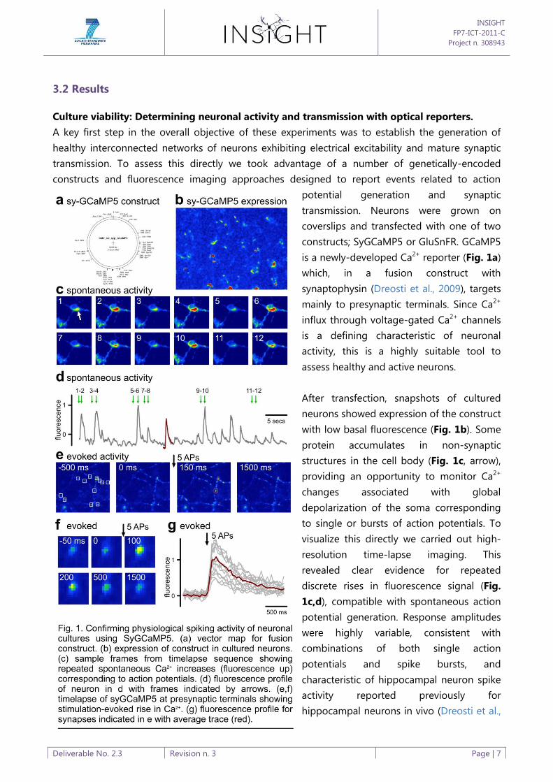
Culture viability: Determining neuronal activity and transmission with optical reporters.
A key first step in the overall objective of these experiments was to establish the generation of
healthy interconnected networks of neurons exhibiting electrical excitability and mature synaptic
transmission. To assess this directly we took advantage of a number of genetically-encoded
constructs and fluorescence imaging approaches designed to report events related to action
potential generation and synaptic
transmission. Neurons were grown on
coverslips and transfected with one of two
constructs; SyGCaMP5 or GluSnFR. GCaMP5
is a newly-developed Ca2+ reporter (Fig. 1a)
which, in a fusion construct with
synaptophysin (Dreosti et al., 2009), targets
mainly to presynaptic terminals. Since Ca2+
influx through voltage-gated Ca2+ channels
is a defining characteristic of neuronal
activity, this is a highly suitable tool to
assess healthy and active neurons.
After transfection, snapshots of cultured
neurons showed expression of the construct
with low basal fluorescence (Fig. 1b). Some
protein accumulates in non-synaptic
structures in the cell body (Fig. 1c, arrow),
providing an opportunity to monitor Ca2+
changes associated with global
depolarization of the soma corresponding
to single or bursts of action potentials. To
visualize this directly we carried out high-
resolution time-lapse imaging. This
revealed clear evidence for repeated
discrete rises in fluorescence signal (Fig.
1c,d), compatible with spontaneous action
potential generation. Response amplitudes
were highly variable, consistent with
combinations of both single action
potentials and spike bursts, and
characteristic of hippocampal neuron spike
activity reported previously for
hippocampal neurons in vivo (Dreosti et al.,
INSIGHT
FP7-ICT-2011-C
Project n. 308943
Deliverable No. 2.3 Revision n. 3 Page | 8
2009). To provide direct evidence to show that rises in SyGCaMP5 signal correspond to neuronal
activity, we imaged presynaptic terminals, visualized as discrete puncta where SyGCaMP5 is
targeted, and stimulated the culture using a field stimulation protocol. A typical time-lapse
sequence (Fig. 1e,f) reveals a robust rise in fluorescence following a brief stimulation protocol
(train of five action-potentials at 20 Hz) at all synaptic terminals (Fig. 1g). Taken together, this
provides clear evidence that neurons are spontaneously active and respond to defined stimulation
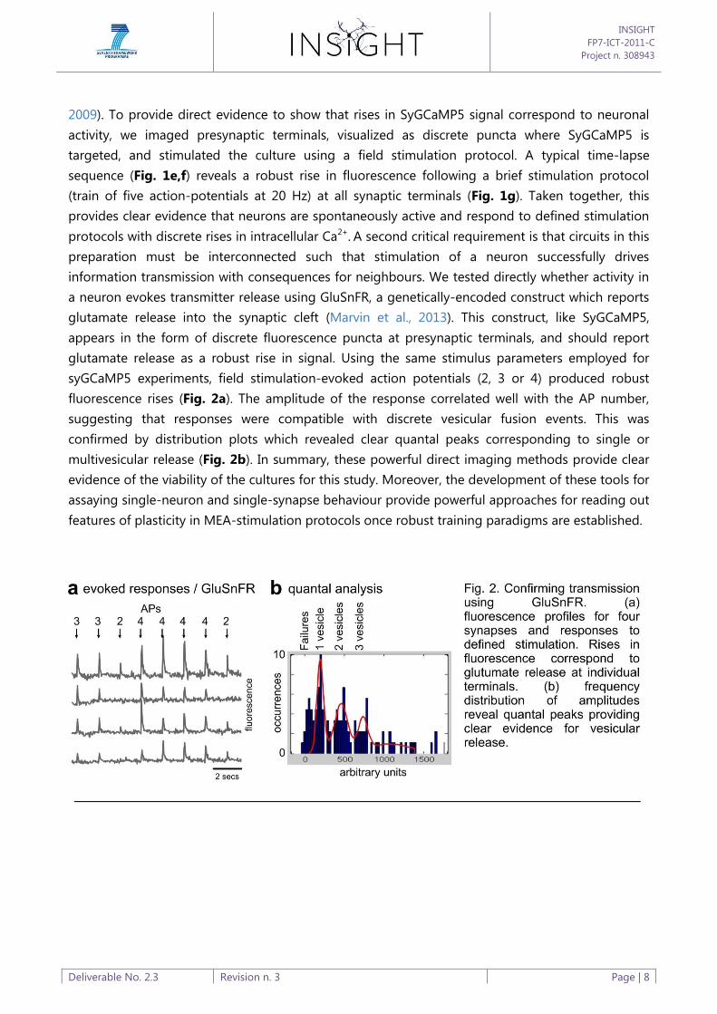
protocols with discrete rises in intracellular Ca2+. A second critical requirement is that circuits in this
preparation must be interconnected such that stimulation of a neuron successfully drives
information transmission with consequences for neighbours. We tested directly whether activity in
a neuron evokes transmitter release using GluSnFR, a genetically-encoded construct which reports
glutamate release into the synaptic cleft (Marvin et al., 2013). This construct, like SyGCaMP5,
appears in the form of discrete fluorescence puncta at presynaptic terminals, and should report
glutamate release as a robust rise in signal. Using the same stimulus parameters employed for
syGCaMP5 experiments, field stimulation-evoked action potentials (2, 3 or 4) produced robust
fluorescence rises (Fig. 2a). The amplitude of the response correlated well with the AP number,
suggesting that responses were compatible with discrete vesicular fusion events. This was
confirmed by distribution plots which revealed clear quantal peaks corresponding to single or
multivesicular release (Fig. 2b). In summary, these powerful direct imaging methods provide clear
evidence of the viability of the cultures for this study. Moreover, the development of these tools for
assaying single-neuron and single-synapse behaviour provide powerful approaches for reading out
features of plasticity in MEA-stimulation protocols once robust training paradigms are established.
INSIGHT
FP7-ICT-2011-C
Project n. 308943
Deliverable No. 2.3 Revision n. 3 Page | 9
4. Developing the MEA recording approach
4.1 MEA Setup
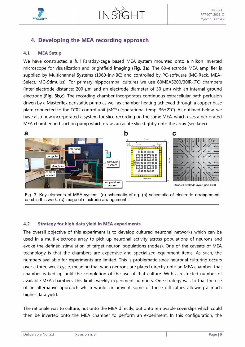
We have constructed a full Faraday-cage based MEA system mounted onto a Nikon inverted
microscope for visualization and brightfield imaging (Fig. 3a). The 60-electrode MEA amplifier is
supplied by Multichannel Systems (1060-Inv-BC) and controlled by PC-software (MC-Rack, MEA-
Select, MC-Stimulus). For primary hippocampal cultures we use 60MEAS200/30iR-ITO chambers
(inter-electrode distance: 200 µm and an electrode diameter of 30 µm) with an internal ground
electrode (Fig. 3b,c). The recording chamber incorporates continuous extracellular bath perfusion
driven by a Masterflex peristaltic pump as well as chamber heating achieved through a copper base
plate connected to the TC02 control unit (MCS) (operational temp: 36±2oC). As outlined below, we
have also now incorporated a system for slice recording on the same MEA, which uses a perforated
MEA chamber and suction pump which draws an acute slice tightly onto the array (see later).
4.2 Strategy for high data yield in MEA experiments
The overall objective of this experiment is to develop cultured neuronal networks which can be
used in a multi-electrode array to pick up neuronal activity across populations of neurons and
evoke the defined stimulation of target neuron populations (nodes). One of the caveats of MEA
technology is that the chambers are expensive and specialized equipment items. As such, the
numbers available for experiments are limited. This is problematic since neuronal culturing occurs
over a three week cycle, meaning that when neurons are plated directly onto an MEA chamber, that
chamber is tied up until the completion of the use of that culture. With a restricted number of
available MEA chambers, this limits weekly experiment numbers. One strategy was to trial the use
of an alternative approach which would circumvent some of these difficulties allowing a much
higher data yield.
The rationale was to culture, not onto the MEA directly, but onto removable coverslips which could
then be inverted onto the MEA chamber to perform an experiment. In this configuration, the

INSIGHT
FP7-ICT-2011-C
Project n. 308943
Deliverable No. 2.3 Revision n. 3 Page | 10
number of coverslips that can be generated in a week is essentially unlimited, and as such, testing a
whole range of conditions to optimize the experiment is highly efficient. Moreover, this strategy
circumvents a major problem; that neurons require an astrocyte feeder layer to support healthy
neuronal growth and synaptic maturation. In the conventional method established in the lab,
coverslips are first coated with a substrate layer (poly-d-lysine) and then astrocytes, and
subsequently followed ~5 days later with the application of neurons onto the astrocyte layer. The
difficulty with using this approach for plating directly onto the MEA is that the astrocytes serve as
an effective insulator shielding the electrodes from direct recording and stimulation of the neurons
(Fig. 4a). The inverted coverslip arrangement circumvents this problem allowing neurons to contact
directly with MEA electrodes while maintaining the integrity of the astrocyte-neuron arrangement.
We first established that this approach was possible using the large, robust and identified neurons
from the mollusc Lymnaea stagnalis. A ganglion was isolated and pressed onto the MEA surface
under a coverslip. We recorded clear and discrete extracellular potentials corresponding to
spontaneous spike activity (Fig. 4b). Using cultured hippocampal neurons (Fig. 4c), inversion of the
coverslip onto the MEA looked visually satisfactory; we saw no evidence to suggest that the
INSIGHT
FP7-ICT-2011-C
Project n. 308943
Deliverable No. 2.3 Revision n. 3 Page | 11
morphological appearance of neurons was compromised by this arrangement (Fig. 4d). Neurons
appeared intact with clear, well-defined cell bodies and processes. Moreover, they are also clearly
in the same focal plane as the electrodes suggesting that they are sitting flat onto the electrode
substrate. Unfortunately, in spite of this promise, the approach proved to be ineffective; it was not
possible to establish robust extracellular recordings from neurons. It is not clear why this is; indeed,
advice from the MEA supplier suggested this should be a sensible and profitable approach.
Presumably the problem relates to the way that neurons adhere to the coverslip with processes
lying flat to the glass and with only the soma approaching the MEA substrate. In this case perhaps,
insufficient neuronal structures contact with electrodes to ensure a signal above noise (Fig. 4e).
4.3 Astrocyte-neuron culture in MEA
In parallel with the above outlined approach we also developed a more conventional strategy for
MEA recording where neurons are applied directly to the MEA chamber. The most challenging
aspect of this was to establish a method which circumvents the difficulties presented by the
astrocytes interfering with the collection of high-fidelity neuronal recordings. There are two
possible solutions to this problem. The first is to grow neuronal cultures in the absence of
astrocytes/glia, a solution established in other labs (Brewer et al., 1993). This is very unsatisfactory,
however. Neuron-only cultures are known to develop and behave very differently to those
supported by glial cells (Eroglu and Barres, 2010), and in recent years substantial concerns have
been raised about the physiological value of this type of culture preparation. In particular, the
important role of astrocytes in plasticity induction and maintenance is now well-established
(Henneberger et al., 2010), and since this is a key aim of the present experiments, this was not a
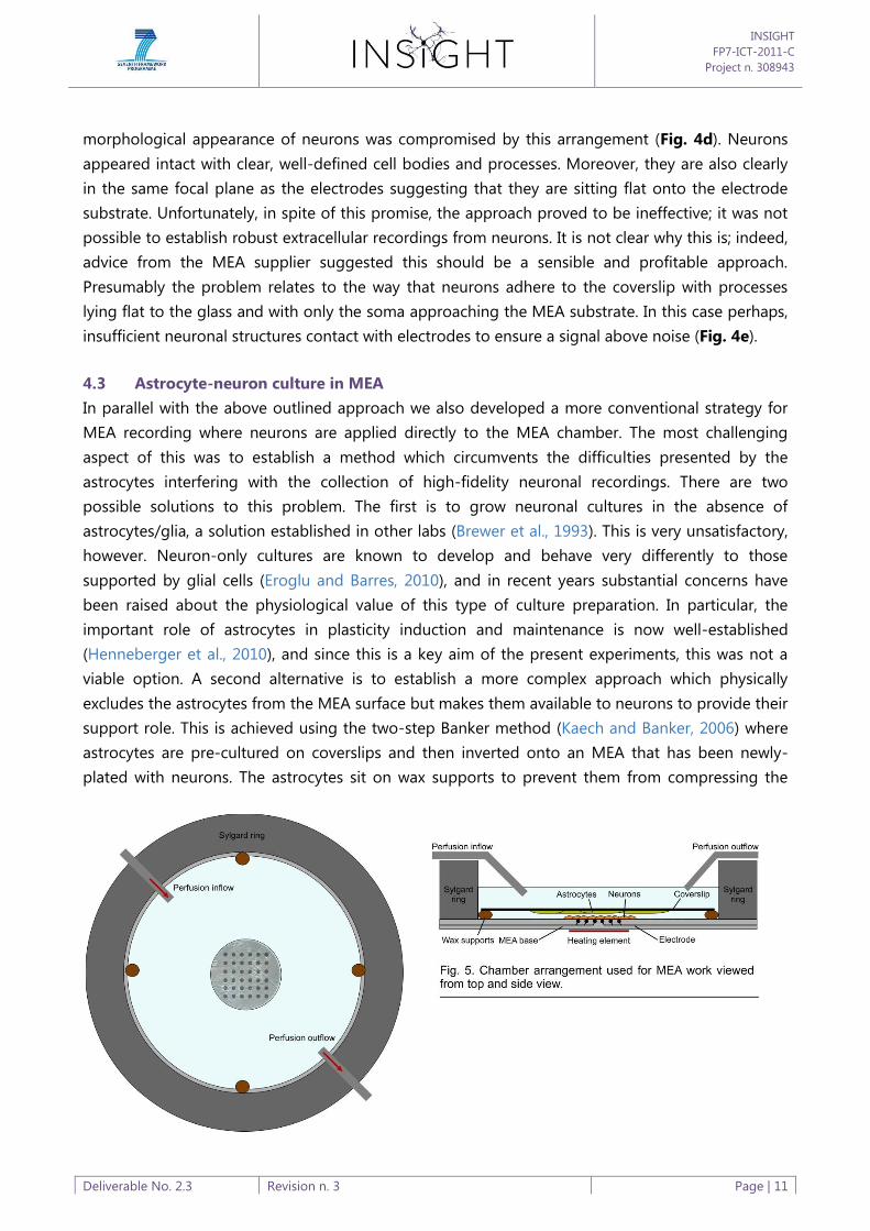
viable option. A second alternative is to establish a more complex approach which physically
excludes the astrocytes from the MEA surface but makes them available to neurons to provide their
support role. This is achieved using the two-step Banker method (Kaech and Banker, 2006) where
astrocytes are pre-cultured on coverslips and then inverted onto an MEA that has been newly-
plated with neurons. The astrocytes sit on wax supports to prevent them from compressing the

INSIGHT
FP7-ICT-2011-C
Project n. 308943
Deliverable No. 2.3 Revision n. 3 Page | 12
neurons and the coverslip is prevented from undergoing lateral drift using a Sylgard block which
holds the coverslip in place. The complete arrangement is shown in (Fig. 4f) and the complete
chamber arrangement in Fig. 5.
Initially we used interconnected networks of hippocampal neurons grown at the density we use in
our imaging experiments (typically ~250 neurons/µl)(Fig. 6a). Although the healthy appearance of
these networks suggested they would produce robust activity, in fact this was not the case. Such
cultures typically showed little or no neuronal activity. Clear stimulus-evoked activation and
network excitability was only reliably seen in cultures plated at high neuronal densities. The
generation of high and very high density cultures (Fig. 6b) provides a technical challenge since the
large area of the whole MEA chamber means that achieving coverage at the necessary density
would require unacceptably high animal usage. To circumvent this, we established an approach
(Fig. 6c) to apply a small high-density droplet to the centre of a dry chamber, pre-treated with PDL,
over the array. Once the neurons had adhered to the substrate, extracellular media was added to
the whole chamber. In this way, a focal region of high-density neurons could be applied selectively
to the centre of the MEA. We found that this approach was critical to the success of the
experiment.
INSIGHT
FP7-ICT-2011-C
Project n. 308943
Deliverable No. 2.3 Revision n. 3 Page | 13

INSIGHT
FP7-ICT-2011-C
Project n. 308943
Deliverable No. 2.3 Revision n. 3 Page | 14
4.4 Activity and stimulation
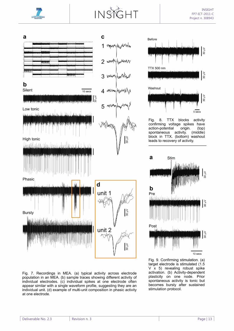
A typical example of activity across 60 electrodes is shown in (Fig. 7a). A unitary event on one
channel appears as a clear deflection above baseline noise. Individual electrodes exhibit a variety of
types of activity (Fig. 7b), including silent, low tonic, high tonic, phasic and bursting activity. In
some cases, activity at one electrode corresponds to one unit defined by a specific waveform (Fig.
7c), while others are comprised of waveform activity with multiple discrete spike shapes (Fig. 7d).
To test that these events do indeed correspond to action potentials, we applied the selective
voltage-gated Na+ channel blocker tetrodotoxin (TTX, 500 nM) to the extracellular solution in a
spontaneously active culture (Fig. 8). As expected, TTX rapidly leads to the silencing of activity and
this is reversible following a washout period. Stimulation of MEAs is achieved by applying a defined
duration and voltage to selected electrodes controlled through the software. Single or multiple
electrodes can be selected in the MCS configuration. Stimulation results in a brief blanking period
on the recording, which serves to protect the amplifier circuit from the stimulation artefact, and a
deflection of the signal from baseline (Fig. 9a). Examples of changes in spontaneous spiking
activity are seen after a repeated stimulation paradigm, suggesting a form of activity-dependent
plasticity has occurred (Fig. 9b). We have now established the basic software-controlled paradigm
for our training experiment to simultaneously stimulate multiple electrodes corresponding to
nodes of activity. As outlined in the full proposal, the initial objective is to train two node networks
(Fig. 10a) using a stimulus paradigm that allows us to explore the encoding and copying of
temporal patterns of activity (Fig. 10b). Success here will see this extended to three-node networks
where the encoding of more complex entrainment patterns can be investigated.
5. MEA for acute slice recording work
We have met the twelve month deliverables for this subproject, establishing the preparation and
recording system necessary to proceed with the next stage of these experiments. We anticipate
that the next six months will yield substantial data. A number of the steps proved more problematic

INSIGHT
FP7-ICT-2011-C
Project n. 308943
Deliverable No. 2.3 Revision n. 3 Page | 15
than expected. In spite of excellent culture viability with robust functionality observed by direct
imaging methods, these parameters did not correlate well with the readouts achievable in MEA.
The solution to this problem was to substantially increase cell density, requiring the development
of a more challenging preparation to ensure good cell viability. A lingering concern is that
connectivity between nodes is often limited. Most pilot experiments were performed at room
temperature and with limited perfusion; these may be key factors that constrain expression of
connected nodes and reduce excitability. Both issues have now been addressed and all future
experiments will be performed in continuously perfused bath solution and at physiological
temperature. However, to circumvent any lingering concerns about the connectedness of the
preparation we have recently established an alternative approach which takes advantage of our
existing set-up alongside a new development in MEA technology; a chamber and suction set-up
allowing activity to be recorded in acute brain slice. This is an important parallel approach since it
provides the opportunity to test the principles of encoding we are examining in primary cultures in
mature native tissue with physiologically-relevant cytoarchitecture. This relies on a perforated MEA
chamber attached to a vacuum pump which holds a tissue slice tightly onto the array by negative
pressure. We have recently developed (see (Marra et al., 2014)) a slice preparation with robust
physiological responses (Fig. 11a-c) and clear evidence for reliable plasticity induction (Fig. 11d).
The transfer of this preparation to the MEA set-up will offer significant further insights into
mechanisms of network plasticity defined in culture in relevant native circuits. We currently await
the arrival of the on-order perforated chamber to test this preparation.
The slice preparation development in the following output which is included in Appendix D:
Marra, V., Burden, J.J., Crawford, F., and Staras, K. (2014). Ultrastructural readout of
functional synaptic vesicle pools in hippocampal slices based on FM-dye-labeling
and photoconversion. Nature Protocols In press.

INSIGHT
FP7-ICT-2011-C
Project n. 308943
Deliverable No. 2.3 Revision n. 3 Page | 16
6. Software Tools for Analysis
6.1 Overview
This section describes the data analysis software developed by the University of Sussex to assist in
quickly summarising and analysing results from the micro-electrode array (MEA) experiments. This
software is critical for expedient analysis of large data sets produced by the experiments, and can
be used to summarise results for use in lab records and publications. It also implements key
analytical algorithms that are part of the experimental data analysis workflow.
During MEA experiments, large amounts of data are produced which record electrical activity on a
neural cell culture through 60 electrode channels. The experiment design involves grouping the
channels into “nodes”, then applying electrical stimulation to the nodes and recording the electrical
activity which is generated by the neurons as a result. Stimulation and recording takes place over
relatively long time scales (several hours) with typically 20-30 GB of data produced per experiment.
This large amount of data presents a challenge for analysis. In order to quickly identify interesting
patterns in the data, the experimenters need access to summary plots and statistics (particularly
raster plots and average spike rates). In particular, we need to identify the interesting data points
(namely the neural spikes), which typically account for only a tiny proportion of the entire data set.
Due to the inherent noise in the recording, the large amount of data, and artefacts introduced in
the time series by the electrical stimulation, this is a non-trivial problem. Short time series plots are
also useful.
The software we have developed aims to solve the needs of the experimenters to have quick access
to the important information. Experiments are conducted frequently, and although various analysis
tools already exist to extract the necessary information, these typically require a time-consuming
process of converting data formats and performing analysis. We also require some custom
algorithms not typically found in pre-packaged software. Analysis from one experiment is typically
needed as soon as possible before more are carried out, in order to guide future work, thus the
software we have developed significantly speeds up a critical path in the experimental workflow.
6.2 Software requirements
After conducting experiments, a large amount of data needs to be processed quickly. Thus speed
(of processing) is a key requirement. Also, the workflow will be sped up by a convenient graphical
interface so that the experimenter can directly access the desired outputs.
The outputs required are:
1. Spike extraction
a. Time series traces of electrical activity must be converted into the time points of
spikes within the series.

INSIGHT
FP7-ICT-2011-C
Project n. 308943
Deliverable No. 2.3 Revision n. 3 Page | 17
b. This essentially a statistical process – there will generally be false positives (noise
misclassified as spikes) and false negatives (spikes which are not extracted). These
need to be kept to a minimum.
c. In order to tune the above to an optimal level, the user must be able to manually
configure the spike extraction parameters.
2. Stimulation
a. Electrical stimulation introduces “artefacts” into the MEA channel data (see below). It
must be possible to locate the stimulation artefacts and identify them as such.
Figure 12: Stimulation artefacts
3. Trace plots
a. It must be possible to show a time series trace of the electrical activity from one or
more of the channel recordings (as above example)

INSIGHT
FP7-ICT-2011-C
Project n. 308943
Deliverable No. 2.3 Revision n. 3 Page | 18
4. Raster plots
a. After extracting spikes, it must be possible to display the time locations of those
spikes as a raster plot, ( see Figure 13)
Figure 13: Example raster plot
b.
(vertical lines indicate presence of a spike at a given time point)
5. Publication plots
a. Plots initially are intended for lab records. However in future we will need the same
plots to be produced in a publication quality form. It must be possible to make the
plots with precise control over the appearance of the result, or to load the data into
alternative plotting software.
6. Merging channels into nodes
a. The initial channels are treated separately. We need to be able to assign a group of
channels to a chosen “node”, and plot those nodes separately, or on the same plot
with different colours.
7. Spike rate averaging
a. We need to calculate and plot the rate of spikes on a channel or node. That is, the
number of spikes per second needs to be calculated over time.

INSIGHT
FP7-ICT-2011-C
Project n. 308943
Deliverable No. 2.3 Revision n. 3 Page | 19
In addition, the software should be extensible in the sense that we may require more complex
types of plots and analysis to be added over time. The design should incorporate the ability to
make additions to the analysis and data visualisation functions of the system.
6.3 Problem analysis
In what follows, methods have been tested for performance on the following two workstations:
Linux workstation
Processor: Quad-core 3.2GHz AMD Phenom II X4 840
Memory: 4GB RAM
Hard disk: SATA III 6Gbps (gigabits per second) Western digital WDC WD10EALX-009BA0.
Quoted maximum transfer rate 126MBps (megabytes per second)1.
Graphics: NVIDIA GeForce GTX 570
Operating system: Ubuntu 13.04 64-bit
Windows workstation
Processor: Dual core 2.7GHz Intel Core i5-3330S
Memory: 4 GB RAM
Hard disk: SATA III 6Gbps Seagate ST1000DM003. Quoted maximum transfer rate 210MBps2
Graphics: Intel HD (integrated)
Operating system: Windows 8.1 64-bit
6.3.1 Data formats
Data is recorded using the MC_Rack software distributed by the manufacturer of the MEA system
we use3. This saves raw data in a proprietary format with extension .mcd (referring to in this report
as a MCD file). The format is not directly accessible from general purpose scientific programming
languages such as MATLAB4 or Python5. Several options were investigated for dealing with the data
format.
6.3.2 Converting raw data with MC_DataTool
The makers of MC_Rack also distribute a data conversion tool, MC_DataTool6, which can read MCD
files and output a few different formats. However, the output types are limited to text files and
Axon Binary format (ABF). Raw electrical data can only be converted to ABF, however ABF is also
not a convenient format for access in general purpose software. Furthermore, ABF can only store 17
channels (and we have recorded 60) in a single file.
1 http://www.wdc.com/global/products/specs/?driveID=894&language=1
2 http://www.seagate.com/staticfiles/docs/pdf/datasheet/disc/barracuda-ds1737-1-1111us.pdf
3 http://www.multichannelsystems.com/software/mc-rack
4 http://www.mathworks.co.uk/products/matlab/
5 https://store.continuum.io/cshop/anaconda/
6 http://www.multichannelsystems.com/software/mc-datatool

INSIGHT
FP7-ICT-2011-C
Project n. 308943
Deliverable No. 2.3 Revision n. 3 Page | 20
6.3.2 Extracting spikes using MC_Rack, then converting with MC_DataTool
The MC_Rack software contains a “spike sorter” module which can be used to extract the locations
of the spikes on each channel from the MCD file. Thus we can use the MC_Rack software to extract
the locations of spikes and brief time windows around each spike. This results in another MCD file
which contains only the spike data (and not the full raw data). This file is much smaller and more
manageable. MC_DataTool can then be used to convert the spike-only data into a text file. This lists
short time series extracts for each spike, representing a 3ms window around the spike point. The
text file can then be fairly straightforwardly read in using a .m script in MATLAB or a Python
function.
This improved on the previous method, but still has a number of drawbacks:
1. The MC_Rack spike extraction module has limited configuration options, and does not
implement the spike extraction approach we have developed (see next section). It must also
be configured by the experimenter for each data set, and since MC_Rack does not produce
the required output plots, it is difficult to verify the correctness of the parameters chosen
quickly.
2. The process of extraction and conversion is a time consuming step.
3. Even though only a relatively small amount of data is produced after spike extraction,
reading text files is a slow process (much slower than reading the binary data files directly),
and so the import into MATLAB or Python is still slow.
6.3.3 Importing data with the Neuroshare framework
Neuroshare7 is a cross platform library for reading common electrophysiology data formats. It can
read MCD files with the plugin library distributed by Multi Channel Systems8. It allows the import of
data into either MATLAB or Python. For preliminary experiments, the Python implementation of
Neuroshare was used9.
The Neuroshare library offers a simple interface to extract data from an MCD file. For example, the
following Python code extracts the first channel that appears in a test file, and displays the first ten
seconds of recorded data.
import neuroshare as ns
fd = ns.File("/home/james/mea data/11022014/data0003.mcd")
#Get first channel
e = fd.get_entity(0)
7 http://neuroshare.sourceforge.net/index.shtml
8 http://www.multichannelsystems.com/software/neuroshare-library
9 http://pythonhosted.org/neuroshare/

INSIGHT
FP7-ICT-2011-C
Project n. 308943
Deliverable No. 2.3 Revision n. 3 Page | 21
#Entire time series
data = e.get_data()
#Plot first 10 seconds of data
plot(data[1][:25000*10],data[0][:25000*10])
The performance of this method was evaluated on the Linux workstation described above. First, we
can establish the data transfer rate from the hard disk (rather than memory cache) by removing all
memory caches:
# echo 3 > /proc/sys/vm/drop_caches
Then testing the time taken to read a 2 GB data file and do nothing with it:
$ time cat data0003.mcd > /dev/null
real 0m16.144s
user 0m0.022s
sys 0m2.888s
Thus it takes approximately 16 seconds just to read the 2 GB of data from the hard disk. After
dropping the caches again, we tested the time taken to read data with Neuroshare:
In [1]: import neuroshare as ns
In [2]: fd = ns.File("/home/james/mea data/11022014/data0003.mcd")
In [3]: %time result = fd.get_entity(0).get_data()
CPU times: user 6.45 s, sys: 3.85 s, total: 10.30 s
Wall time: 21.44 s
In [4]: %time result = fd.get_entity(1).get_data()
CPU times: user 5.73 s, sys: 1.14 s, total: 6.87 s
Wall time: 8.19 s

INSIGHT
FP7-ICT-2011-C
Project n. 308943
Deliverable No. 2.3 Revision n. 3 Page | 22
In [5]: %time result = fd.get_entity(2).get_data()
CPU times: user 5.79 s, sys: 1.27 s, total: 7.06 s
Wall time: 9.31 s
Thus the first read of an entire channel takes approximately 21 seconds, slightly longer than it takes
just to read (all 60 channels of) the data from the hard disk. Subsequent reads take 8-9 seconds per
channel, since the file is cached in memory by the operating system after the first access. Thus
reading all 60 channels by this method is likely to take around 8 minutes.The speed of this method
is likely to be a significant drawback. Furthermore we could not get the Neuroshare library for
Windows to work. Since the computers used by the experimenters are running Windows this would
be a problem.
Another drawback of Neuroshare is that data is imported in 64-bit double precision floating point
format, after converting from the 16-bit integer format used internally by the MCD data files. This
quadruples the memory requirements of the imported data, and is likely to be a major cause of the
slowdown in reading data. For handling large data, it would be preferable to maintain the more
manageable 16 bit data format. Neuroshare does not provide a way to do this.
6.3.4 Reading data with the MC_Stream C++ library
MC_Rack is distributed with a C++ library which can be directly used to read MCD files at a low
level. The output from this library is given in the native 16-bit integer format. The drawback is that
there is no direct way to interface this output with MATLAB or Python. We needed to develop a
Python module which makes use of the provided C++ library to access the MCD files (see section
“mcdfile library” below).
However, direct access to the MC_Stream library allows us to have more flexibility in how the files
are read. For example, using our custom Python module mcdfile, extracting the entire data set from
a 2 GB file takes 37 seconds on the test Linux machine:
In [1]: import mcdfile
In [2]: fd = mcdfile.McdFile("/home/james/mea data/11022014/data0003.mcd")
In [3]: %time data = fd.getAllData(0)
CPU times: user 1.41 s, sys: 6.10 s, total: 7.51 s
Wall time: 37.74 s
In the above process, the entire data file is read into a secondary disk location by the function
getAllData. The parameter 0 to this function specifies the stream ID – streams are data structures
within the MCD file that store separate recordings. For our purposes, we only store one recording
per MCD file (separate channels are recorded at the same time and thus are counted as one data
INSIGHT
FP7-ICT-2011-C
Project n. 308943
Deliverable No. 2.3 Revision n. 3 Page | 23
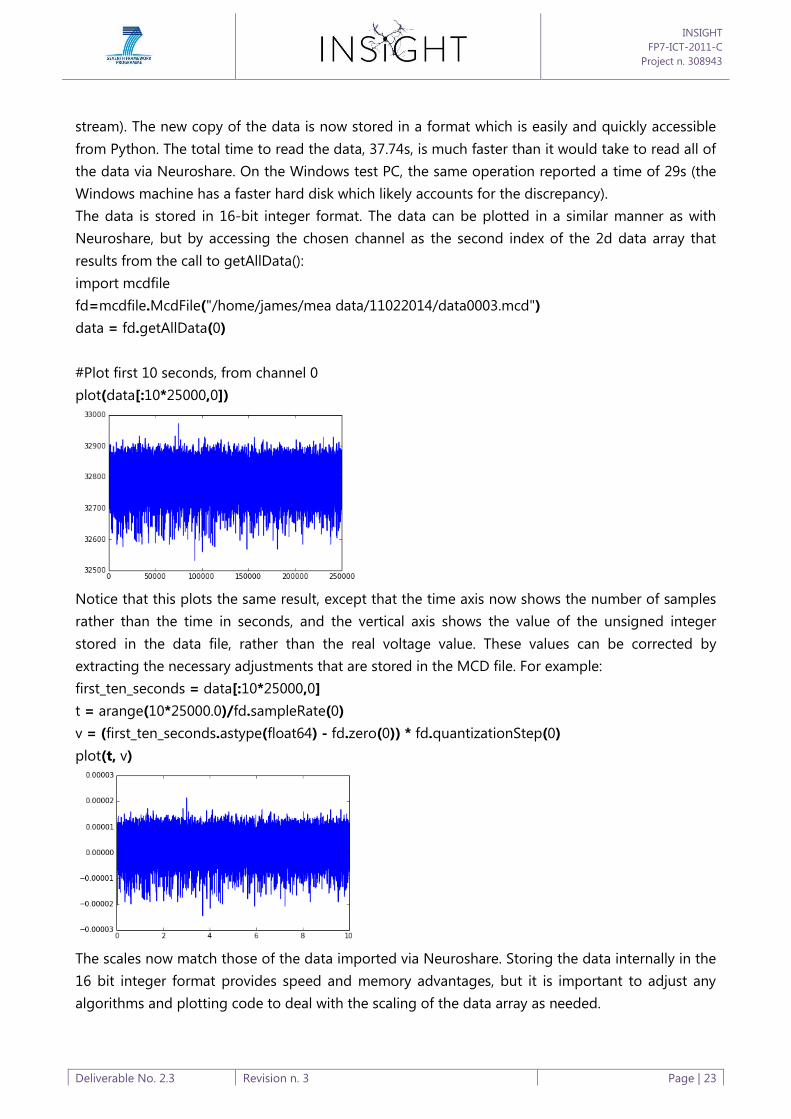
stream). The new copy of the data is now stored in a format which is easily and quickly accessible
from Python. The total time to read the data, 37.74s, is much faster than it would take to read all of
the data via Neuroshare. On the Windows test PC, the same operation reported a time of 29s (the
Windows machine has a faster hard disk which likely accounts for the discrepancy).
The data is stored in 16-bit integer format. The data can be plotted in a similar manner as with
Neuroshare, but by accessing the chosen channel as the second index of the 2d data array that
results from the call to getAllData():
import mcdfile
fd=mcdfile.McdFile("/home/james/mea data/11022014/data0003.mcd")
data = fd.getAllData(0)
#Plot first 10 seconds, from channel 0
plot(data[:10*25000,0])
Notice that this plots the same result, except that the time axis now shows the number of samples
rather than the time in seconds, and the vertical axis shows the value of the unsigned integer
stored in the data file, rather than the real voltage value. These values can be corrected by
extracting the necessary adjustments that are stored in the MCD file. For example:
first_ten_seconds = data[:10*25000,0]
t = arange(10*25000.0)/fd.sampleRate(0)
v = (first_ten_seconds.astype(float64) - fd.zero(0)) * fd.quantizationStep(0)
plot(t, v)
The scales now match those of the data imported via Neuroshare. Storing the data internally in the
16 bit integer format provides speed and memory advantages, but it is important to adjust any
algorithms and plotting code to deal with the scaling of the data array as needed.

INSIGHT
FP7-ICT-2011-C
Project n. 308943
Deliverable No. 2.3 Revision n. 3 Page | 24
The mcdfile library provides access to other important details about the recording as the following
code snippet illustrates:
In [1]: import mcdfile
In [2]: fd=mcdfile.McdFile("/home/james/mea data/11022014/data0003.mcd")
In [3]: fd.channelCount(0)
Out[3]: 60L
In [4]: fd.channelName(0,0)
Out[4]: '47'
In [5]: fd.channelName(0,1)
Out[5]: '48'
In [6]: fd.startTime()
Out[6]: '2014-02-11 11:47:52.851'
Detailed descriptions of these functions are given in the mcdfile module documentation below (
see APPENDIX A ). The downside of this approach is that it requires a more involved amount of
newly written code to interface with the C++ library. However, the results appear to be generally
much faster. There is also no need to convert file formats before use, and the Python module was
tested and found to work on Windows so this was deemed to be a good solution.
6.4 Spike extraction approach
A number of approaches for locating spikes within the data were evaluated. This section describes
the current technique we use.
Typical spike extraction methods work one of two ways: either by simple thresholds, where a spike
is assumed to occur whenever the voltage passes a chosen threshold in a particular direction, or by
voltage slope, where a spike is counted every time the voltage changed by a certain amount in a
specified time window. These two approaches can be chosen in the MC_Rack spike sorter tool, for
example.
A common problem with the data obtained from the MEA is that the stimulation introduces
artefacts which introduce long transients over which the spikes appear as shown below (Figure 14) ,
from a section of recording taken a few milliseconds after a stimulation has occurred:

INSIGHT
FP7-ICT-2011-C
Project n. 308943
Deliverable No. 2.3 Revision n. 3 Page | 25
Figure 14: Example trace showing long term transient introduced by stimulation artefact
The downward slope is introduced by stimulation. Notice that several spikes appear, which have a
total peak to peak amplitude of around 60-70µV, typically with a negative peak relative to the
“baseline” of around -30µV. However, due to the transient slope, they do not all pass the lower -
30µV absolute voltage level, ruling out absolute thresholding.
Voltage rate thresholding is an improvement, as it is less dependent on the baseline level of the
voltage. However, it also proved inadequate for us as the stimulation artefacts and background
noise sometimes contain sharp differentials which can be misclassified as spikes.
Thus our approach works in several stages, the first of which is a normal voltage rate threshold. The
algorithm is as follows:
1. Starting at time (starting at the beginning of the recording for a given channel),
determine if the voltage difference ( ) ( ) is within the
range ( ).
a. If so, construct a 3ms window around the threshold point:
( )
b. Find the negative peak of the spike within the 3ms window around .
( )
c. Calculate the difference of the peak voltage to the median voltage of the window.

INSIGHT
FP7-ICT-2011-C
Project n. 308943
Deliverable No. 2.3 Revision n. 3 Page | 26
( ) median( ( ) )
d. If we have both relative and absolute voltages within specified ranges:
( ) ( ) ( )
i. Then record the time and voltage ( ) as a spike event.
ii. Set the next time point to (i.e. skip a short period after the
detected spike) and return to step 1.
2. (No spike detected) set to the next available time sample and return to step 1.
The algorithm requires the following parameters. A reasonable choice is shown below but it can be
adjusted at any time to affect the sensitivity and specificity (number of false negatives and
positives). This can be necessary if different recordings suffer from different noise levels or exhibit
different spike voltages, though most are close to this range.
Parameter Description Initial
value
Min. voltage difference -100.0µV
Max. voltage difference -20.0µV
Voltage difference timing 0.5ms
Min. absolute peak -100.0µV
Max. absolute peak 50.0µV
Min. peak relative to baseline -100.0µV
Max. peak relative to
baseline
-30.0µV
Table 1: List of parameters for spike extraction algorithm
The use of the absolute voltage cut-off allows us to ensure that peaks that are clearly due to the
large stimulation artefacts will always be ignored. The relative voltage cut-off gives a better idea of
the peak amplitude of a spike, making use of all the available data within the 3ms window to
calculate a baseline, whereas the initial voltage rate effectively treats a single time point as the
baseline for comparison, which can be affected by noise easily. However, using the naïve voltage
rate threshold as an early “screen” to the algorithm means that we do not have to calculate median
values for voltage windows throughout the entire data set, which would be extremely time
consuming.
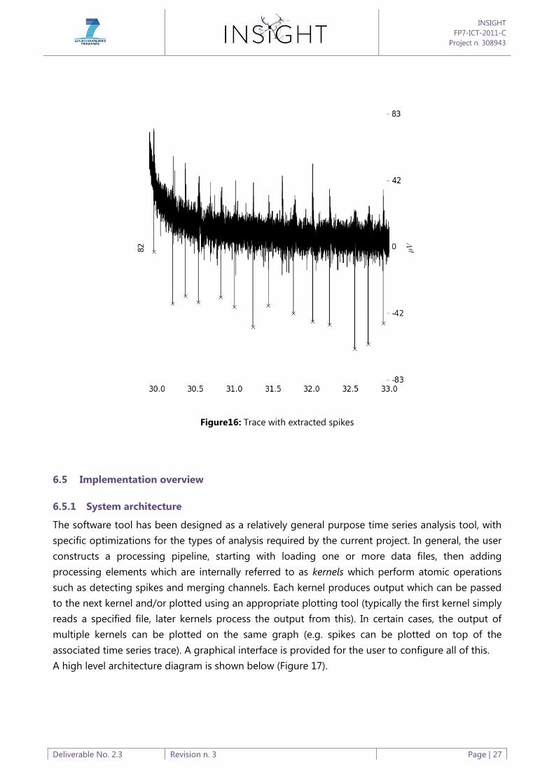
Since the voltage and time point of a peak are recorded, we can see the output of the full
algorithm by plotting spike points on top of the time series trace as marked points, for example as
below (Figure 16):
INSIGHT
FP7-ICT-2011-C
Project n. 308943
Deliverable No. 2.3 Revision n. 3 Page | 27
Figure16: Trace with extracted spikes
6.5 Implementation overview
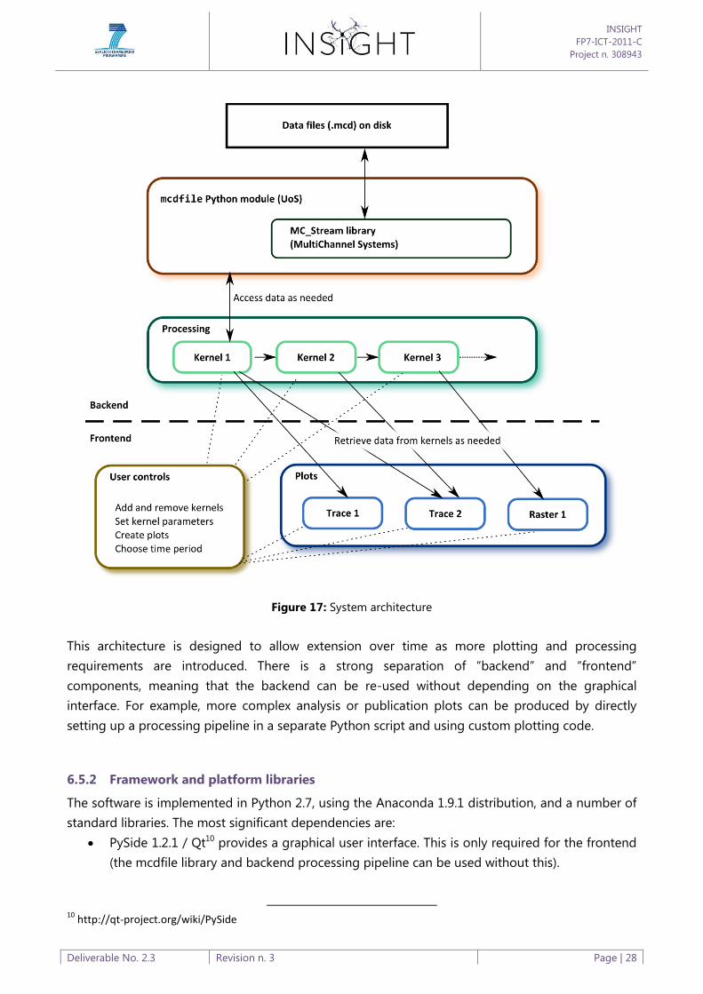
6.5.1 System architecture
The software tool has been designed as a relatively general purpose time series analysis tool, with
specific optimizations for the types of analysis required by the current project. In general, the user
constructs a processing pipeline, starting with loading one or more data files, then adding
processing elements which are internally referred to as kernels which perform atomic operations
such as detecting spikes and merging channels. Each kernel produces output which can be passed
to the next kernel and/or plotted using an appropriate plotting tool (typically the first kernel simply
reads a specified file, later kernels process the output from this). In certain cases, the output of
multiple kernels can be plotted on the same graph (e.g. spikes can be plotted on top of the
associated time series trace). A graphical interface is provided for the user to configure all of this.
A high level architecture diagram is shown below (Figure 17).
INSIGHT
FP7-ICT-2011-C
Project n. 308943
Deliverable No. 2.3 Revision n. 3 Page | 28
Figure 17: System architecture
This architecture is designed to allow extension over time as more plotting and processing
requirements are introduced. There is a strong separation of “backend” and “frontend”
components, meaning that the backend can be re-used without depending on the graphical
interface. For example, more complex analysis or publication plots can be produced by directly
setting up a processing pipeline in a separate Python script and using custom plotting code.
6.5.2 Framework and platform libraries
The software is implemented in Python 2.7, using the Anaconda 1.9.1 distribution, and a number of
standard libraries. The most significant dependencies are:
PySide 1.2.1 / Qt10 provides a graphical user interface. This is only required for the frontend
(the mcdfile library and backend processing pipeline can be used without this).
10
http://qt-project.org/wiki/PySide
INSIGHT
FP7-ICT-2011-C
Project n. 308943
Deliverable No. 2.3 Revision n. 3 Page | 29
Numpy 1.8.0 / Scipy 0.13.311 provides array storage formats and basic scientific
computation routines. The Numpy array and structured array formats are used internally for
all data streams (see next section). Numpy also provides file save and load operations used
to store extracted data (see NPZ File) section. The memory mapping function of Numpy is
also used in the mcdfile library (see mcdfile library section).
Matplotlib 1.3.112 is a plotting framework which provides highly customizable scientific
plotting tools which can be integrated into the PySide interface straightforwardly.
Cython 0.20.113 is a tool that compiles a modified Python language into C++ code that can
be loaded as modules into Python programs. This is used to implement the mcdfile library
as it allows interfacing C++ and Python classes. It is also used to provide a faster
implementation of the spike extraction algorithm, since it can produce optimized C++ code
which can run faster than a Python implementation.
6.5.3 Internal data formats
There are two “types” of time series data that are passed through the processing chain, raw
(continuous data) and sparse (where an array of time locations of events are recorded along with a
corresponding array of values for each event, for example spike times and spike peaks).
As noted earlier, the MCD file format stores recordings as unsigned 16 bit integers. This are offset
from zero by a value that can be extracted from the MCD file (generally this appears to be half the
available range, i.e. 215 = 32768). For simplicity of internal calculations, while retaining the speed
and memory benefits of the 16 bit representation, these are converted on loading to signed 16 bit
integers centred around zero. Thus all raw data streams internally are signed 16 bit integer arrays.
The processing pipeline must still store the quantization step and sample rate information required
to convert these to real values (see below).
Sparse data streams consist of Numpy structured arrays, with a field “t” giving the event time in
real time (as a floating point time in seconds, generally the start of a recording is treated as 0.0
seconds), and a field “x” which is a signed 16 bit integer in the same manner as the raw data
streams (e.g. it will often be the spike peak value). The array will thus be only as long as the number
of events stored (whereas a raw data array is as long as the total amount of time represented
multiplied by the sample rate).
6.5.4 Processing Pipeline
The processing pipeline consists of a series of user configured kernels arranged in a chain, where
each kernel maintains a reference to the previous kernel in the chain. Each of the kernels is a
11
http://www.numpy.org/ 12
http://matplotlib.org/ 13
http://cython.org/

INSIGHT
FP7-ICT-2011-C
Project n. 308943
Deliverable No. 2.3 Revision n. 3 Page | 30
Python class which implements a specified type of operation, such as loading data from a file. The
classes may be instantiated and parameters set (e.g. the filename to load).
A particular kernel class has a fixed input data type and output data type, though the input type
may be irrelevant. For example, the MCD file loading kernel has no meaningful input type, and its
output type is raw since it produces continuous time series data. The spike extraction kernel has an
input type of raw and an output type of sparse, since it processes continuous data and outputs a
sparse set of spike events.
Each kernel provides access to a single recording, which consists of a set of channels with data
available in a given time window. A kernel must provide a method with the following signature:
get_data(channel_list, t0, length)
The channel_list argument is a Python list with the names of the channels to access. The t0 and
length parameters accept “real” time points as a floating point representations in seconds (with t0
being the seconds since the start of the recording). The method returns a Python list with entries
corresponding to the input channel list, where each entry contains the data for that channel, in
either the raw or sparse data format outlined above, depending on the output type of the kernel.
Where kernels need to access data from previous kernels in the chain, they maintain a reference to
their parent kernel. They can then call get_data on the parent kernel as required. Furthermore any
secondary fields (for example the list of available channels, the sample rate, etc) are by default
automatically inherited from the parent kernel (though a kernel can replace them as desired).
A kernel’s parent must always have an output type which matches the input type of the kernel. If
the immediate predecessor kernel in the chain does not have the appropriate output type, the
kernel will look further back in the chain for the first available predecessor with the appropriate
output type.
For example, the figure below (Figure 18) illustrates what happens if an MCD File kernel is loaded
first, and then “Extract stimulations” and “Extract spikes” are added to the chain. Both the
subsequent kernels require a raw data input, but when the “Extract spikes” kernel is added, its
immediate predecessor in the chain (“Extract stimulations”) has an output type of sparse. Thus the
spike kernel is “re-parented” to the MCD File kernel, so it accesses the same original raw data for
calculating spikes. Properties such as sample rate are also inherited directly from the MCD file
kernel.

INSIGHT
FP7-ICT-2011-C
Project n. 308943
Deliverable No. 2.3 Revision n. 3 Page | 31
Figure 18: Example processing chain
6.5.5 Kernels
The kernels currently available in the system are listed below. The kernels can be found in
kernels.py in the source code.
Name Class Description Input type Output
type
MCD File McdFile Load data from MCD file <Irrelevant> Raw
NPZ File NpzFile Load data from NPZ file <Irrelevant> Sparse
Extract
spikes
SpikeExtract Locate spikes in raw data (using
algorithm described above)
Raw Sparse
Extract
stimulations
StimExtract Locate stimulation events in
data
Raw Sparse
Spike rate SpikeRate Calculate the average frequency
of spikes in time windows
Sparse Raw
Merge spike
channels
MergeSpikes Copy spikes from a group of
input channels to a single, newly
created output channel
Sparse Sparse
Table 2: List of kernels

INSIGHT
FP7-ICT-2011-C
Project n. 308943
Deliverable No. 2.3 Revision n. 3 Page | 32
6.5.6 Plots
Plot functions are available to the user and create plot classes in the graphical interface portion of
the code (currently found in main.py in the source code). Plots are configured with a set of
channels to read from specified kernels. Each channel can be assigned a “group”, so that, for
example, difference groups can be plotted in different colours. There are currently two plot classes:
Trace plot
This can plot both raw and sparse channels. Raw data is plotted as a continuous trace, sparse data
is overlayed with “x” markers. The example below shows two channels with both the original
voltage trace and extracted spikes overlaid (see Figure 19).
Figure 19: Example trace plot
Raster plot
Raster plots show only sparse data. Each event is plotted as a vertical line, with multiple channels
shown on a single graph as in the example below (Figure 20).

INSIGHT
FP7-ICT-2011-C
Project n. 308943
Deliverable No. 2.3 Revision n. 3 Page | 33
Figure20: Example raster plot
6.5.7 NPZ file specification
The user has the option to save any sparse time series to an NPZ file. This is useful because
typically the spike extraction process takes a while on large data sets. A set of spikes can be saved
to an NPZ file, which is typically only a few kB, and these can be loaded quickly for later analysis.
The NPZ file is created using the numpy.savez14 function. This places several data structures into a
single file, each given an identifying name. The file can later be loaded via the numpy.load function.
The NpzFile kernel wraps numpy.load15 to provide the file data to the processing chain.
NPZ files created by the MEA Analysis software contain the following data structures:
sample_rate – single integer with the original sample rate of the data.
quantization_step – floating point quantization step from the original data.
time_limits – a pair of floating points (start time and stop time)
channels – a dictionary of channel name to sparse data structures
Further details of the software tools can be found in Appendix A (mcd file library description), Appendix B
(software build process) and Appendix C (user guide).
14
http://docs.scipy.org/doc/numpy/reference/generated/numpy.savez.html 15
http://docs.scipy.org/doc/numpy/reference/generated/numpy.load.html

INSIGHT
FP7-ICT-2011-C
Project n. 308943
Deliverable No. 2.3 Revision n. 3 Page | 34
7. Causal Inference
This section outlines work investigating modern approaches to inferring causation that may be
applicable within the context of the INSIGHT project and with wider scientific relevance. In
particular these methods will be applied to the analysis of data from the experiments on the
learning of causal relationships in spiking neural networks which will be carried out in the next
phase of the project.
7.1 Background information: inferring causation
This section summarises some background information on concepts of causation and can be
skipped by those who are familiar with the area.
The question of how to infer causes has recently developed into a major subject of interest in a
number of fields. In psychology, humans are thought to make causal judgements about the world
around them (Griffiths and Tenenbaum, 2005). In work directly related to the INSIGHT project, it
has been proposed that an ability of neural circuits to perform causal learning could offer a
mechanism for the copying required by some versions of the neuronal replicator hypothesis
(Fernando 2013).
There are a number of proposals for models of causal learning inspired by rational agent models.
Supposing that an agent receives information about the occurrence of two types of event, where
one is considered a putative cause c, and the other the putative effect e. The occurrence of c is
denoted and non-occurrence , likewise for and . Then the information about the
number of occasions when the events occurred or did not occur in the possible combinations is
what a statistician would refer to as a contingency table, where for example ( ) refers to the
number of occasions that a occurred but an did not:
Totals
( ) ( ) ( )
( ) ( )
( ) ( ) ( )
( ) ( )
Totals ( ) ( )
( )
( ) ( )
( ) N (total number of
events)
Making a decision as to the strength of evidence that c causes e based on this information is called
an elementary causal judgement (Griffiths and Tenenbaum, 2005). Elementary in the sense that just
two types of event are considered (more complex models may consider a wider variety of
possibilities, such as common causes between variables).
INSIGHT
FP7-ICT-2011-C
Project n. 308943
Deliverable No. 2.3 Revision n. 3 Page | 35
Two influential proposals for estimating causal influences are based on conditional probabilities
that can be estimated from contingency table data. The probability of the occurrence of an A
conditioned on prior knowledge that B also occurred ( ) is defined empirically as:
( ) ( )
( )
The first proposal is (Jenkins and Ward, 1965):
( ) ( )
i.e. the difference in conditional probabilities of the occurrence of a c, depending on whether an e
also occurred. An alternative model is suggested by Cheng (1997) who notes that does not
account for whether e also occurs when c does not. Cheng’s alternative is causal power CP:
( )
With some re-arranging this is:
( )
( )
( )
( )
Thus causal power higher according to the first term when the effect is very likely to occur in
combination with the cause, and unlikely to occur without the cause, and is also reduced by the
second term if the effect is very likely to happen irrespective of the occurrence of the cause.
In more complex scenarios, causal relationships are often analysed according to probabilistic
conditioning effects. This approach has been developed in several, sometimes independent
strands, particularly by Reichenbach (1951), Granger (1969, who credits the influence of Norbert
Wiener), Suppes (1970), Salmon (1970) and recently developed in theories of causal Bayes nets
(Spirtes et al, 2001, Pearl, 2009). This is the idea that causes can be related to their effects if a
correlation obtains even when all possible background and mediating factors have been conditioned
out. This is formulated in a variety of ways, a typical approach being to say that causes must be
correlated with their effects in (one or all, depending on the formulation) causally homogeneous
populations (i.e. sets of individuals where all causally relevant background factors are statistically
identical). E.g. c is said to cause e if:
( ) ( )
Where is the state of all the causally relevant background factors in the causally homogeneous
population subgroup . This is the concept of causation that underlies many modern scientific
practises such as randomised controlled trials (where it ensured that is identical between the
treatment group where occurs, and the control group which receives , through randomisation
and blinding if necessary, Cartwright, 2007). It is also closely related to Granger’s (1969) conception,
intended for analysis of time series, which can be roughly stated as:
( ) iff ( )
Read “X (Granger-)causes Y if and only if the present state of X is correlated with the future state of
Y conditional on the entire history of the universe, except for X, up to the present”. Since it is
impractical to measure the entire state of the universe, Granger proposes a more modest definition
for practical needs:
( ) iff ( )
INSIGHT
FP7-ICT-2011-C
Project n. 308943
Deliverable No. 2.3 Revision n. 3 Page | 36
Where the prior state of the universe except for X is approximated by the prior state of the putative
effect variable Y.
Similarly, the Bayes nets approaches of Spirtes et al. (2001) and Pearl (2009) are founded on the
principle that conditioning on common causes and mediating factors must remove correlations
between variables, unless there is some alternative causal pathway (i.e. a direct causal connection)
between those variables which has not been accounted for (Granger’s approach is simply a specific
case of this, where “all common causes” are assumed to be accounted for by the history of the
universe, not including the putative cause itself). Causal Bayes nets encode the causal relationships
between variables on a directed acyclic graph, where each variable is identified with a node, and the
relationship “A causes B” is encoded by an arrow from A to B. Facts about the probabilistic
dependencies between variables can be “read off” from the causal graph according to algorithmic
rules that relate the node and arrow structures in the graph to properties of compatible probability
distributions.
Multiple causal hypotheses can therefore be encoded in distinct causal graphs representing the
underlying causal relationships in the world. Griffiths and Tenenbaum (2005) propose that rather
than or causal power, causal inferences are made by assigning preference to one out of a set of
causal graphs. They argue that this distinguishes between causal structure (the presence or absence
of causal connection in the graph) and causal strength. The causal support (CS) is proposed by
Griffiths and Tenenbaum (2005), and is the Bayes factor associated with the graph containing a
causal influence relative to one that does not contain that influence:
( )
( )
Where D is the data available to the agent, and and are competing causal models
(in the case of an elementary causal judgement, show an arrow between c and e, and
does not. It is this latter approach that Fernando (2013) shows can be encoded using a
neural network simulation. An agent (or neural network) which adopts this approach to determine
the true causal relationships determining its sensory data would be performing a kind of Bayesian
learning.
7.2 Causality measures
We have investigated approaches to measuring causality, in particular in the context of embodied
agents. This feeds into our understanding of the nature of various proposals for detecting and
measuring causal relationships, particularly in the context of temporally specific information. A
paper described below describes how information transfer relates to causal influences in a simple
embodied agent. Ongoing work is looking at a comparison of a variety of proposed “causality
detecting” algorithms, and introduces a novel variant of Sugihara et al’s (2012) “convergent cross
mapping” with desirable properties. This informs our work in the area of encoding causal

INSIGHT
FP7-ICT-2011-C
Project n. 308943
Deliverable No. 2.3 Revision n. 3 Page | 37
information in spiking neural networks, since there are a number of important aspects of current
theories of causation that will impinge on our future work.
7.3 Information transfer in embodied agents
In one strand of this work, we have investigated the information transfer, a generalisation of
Granger causality, in embodied agents. A paper presented at the European Conference on Artificial
Life (2013):
Project output - Thorniley, J., & Husbands, P. (2013). Hidden information transfer in
an autonomous swinging robot. In Advances in Artificial Life, ECAL 2013 (Vol. 12, pp.
513–520). MIT Press. doi:10.7551/978-0-262-31709-2-ch074
describes some of our recent work in this area. This paper (Thorniley and Husbands, 2013)
describes a hitherto overlooked aspect of the information dynamics of embodied agents, which can
be thought of as hidden information transfer. This phenomenon is demonstrated in a minimal
model of an autonomous agent. While it is well known that information transfer is generally low
between closely synchronised systems, here we show how it is possible that such close
synchronisation may serve to “carry” signals between physically separated endpoints. This creates
seemingly paradoxical situations where transmitted information is not visible at some intermediate
point in a network, yet can be seen later after further processing.
Information transfer was measured between different variables of a simulated physical system
representing an agent swinging on a swing. The state of the agent’s control system (brain) is
represented by the variable u, its body state consists of two variables, r and v (body extension and
velocity), and the environment, namely the swing is represented by the variables and (rotation
and angular velocity). Information transfer was calculated between all variables in a variety of
behaviour modes, with representative plots shown in Figure 21 below.
Figure 21: Information transfer between components of a swinging agent under different behavioural
regimes. Figure from Thorniley and Husbands (2013)
INSIGHT
FP7-ICT-2011-C
Project n. 308943
Deliverable No. 2.3 Revision n. 3 Page | 38
A particularly interesting result is shown in (b) – where the agent is swinging. The thick red arrows
show high information transfer from the brain and body variables (u, v and r) to the environment
variables ( and ). In particular there is high information transfer from u to and , in spite of the
fact that there is low information transfer from u to r and v. This defeats the causal intuition around
information transfer, because the physical nature of the model is such that the brain cannot
possibly influence the state of the world without first influencing the state of the body. We
hypothesise that this is because very strong relationships may actually induce low information
transfer, since they reduce the overall variation in the system. All information measures require that
there is some random variation in the system, in order to determine if that variation (for example in
a causal variable) is “picked up” in another variable. The strong entrainment of body and brain
dynamics may remove this necessary variation.
7.4 Causality detectors
There have been many recent proposals for “causality detecting” algorithms that can be applied to
time series. We have developed a reference implementation of several. Many derive from the
notable proposal of Granger (1969) (see background information), though a recent suggestion by
Sugihara et al (2012) is substantially different.
The Granger-causality concept, as discussed in the introduction, suggests that causes should be
correlated with their effects conditional upon the past histories of those effects. Transfer entropy
(Schreiber, 2000) is a generalisation of this using information theoretic analysis (Barnett, 2009). A
difficulty with transfer entropy is estimating probability distributions where the data are
continuous-valued. Naïve binning tends to have poor performance. Two preferable solutions are
nearest-neighbour based estimation (Kraskov et al, 2004) and symbolic transfer entropy (STE,
Staniek and Lehnertz, 2008).
Sugihara et al’s (2012) convergent cross mapping (CCM) is substantially different both in theory and
practice. It proposes that since causal variables “drive” their effects, and thus the causal variable
should be detectable from the dynamics of the effect variable. This is particularly suited to analysis
of dynamical systems, for which Taken’s (1981) theorem states that a suitable delay-embedding of
a single variable from a multi-variable system should contain all of the information about the
current dynamical regime of the entire system. Thus, if one variable “drives” another, a delay
embedding of the driven (effect) variable should be predictive of the driver (cause) variable.
We have compared CCM and several types of transfer entropy on simulated dynamical systems.
Importantly, we also conjecture that CCM is closely related to, in fact essentially a biased estimate
of, time delayed mutual information. This result is likely to be significant, as it demonstrates that a
poorly understood measure (CCM) can be related to a more mathematically well-defined statistic
(mutual information). We are preparing a publication along these lines.
INSIGHT
FP7-ICT-2011-C
Project n. 308943
Deliverable No. 2.3 Revision n. 3 Page | 39
References
Brewer, G.J., Torricelli, J.R., Evege, E.K., and Price, P.J. (1993). Optimized survival of hippocampal
neurons in B27-supplemented Neurobasal, a new serum-free medium combination. J Neurosci Res
35, 567-576.
Cartwright, N. (2007). Are RCTs the gold standard? BioSocieties, 2(1), 11–20. Retrieved from
http://www.palgrave-journals.com/biosoc/journal/v2/n1/abs/biosoc20072a.html
Cheng, P. W. (1997). From covariation to causation: A causal power theory. Psychological Review,
104(2), 367–405. doi:10.1037//0033-295X.104.2.367
Darcy, K.J., Staras, K., Collinson, L.M., and Goda, Y. (2006). Constitutive sharing of recycling synaptic
vesicles between presynaptic boutons. Nat Neurosci 9, 315-321.
Dreosti, E., Odermatt, B., Dorostkar, M.M., and Lagnado, L. (2009). A genetically encoded reporter of
synaptic activity in vivo. Nat Methods 6, 883-889.
Eroglu, C., and Barres, B.A. (2010). Regulation of synaptic connectivity by glia. Nature 468, 223-231.
Fernando, C. (2013). From Blickets to Synapses: Inferring Temporal Causal Networks by
Observation. Cognitive Science, 1–45. doi:10.1111/cogs.12073
Fidjeland, A. K., Gamez, D., Shanahan, M. P., & Lazdins, E. (2013). Three tools for the real-time
simulation of embodied spiking neural networks using GPUs. Neuroinformatics, 11(3), 267–90.
doi:10.1007/s12021-012-9174-x
Goodman, D., & Brette, R. (2008). Brian: a simulator for spiking neural networks in python. Frontiers
in Neuroinformatics, 2(November), 5. doi:10.3389/neuro.11.005.2008
Granger, C. W. J. (1969). Investigating Causal Relations by Econometric Models and Cross-spectral
Methods. Econometrica, 37(3), 424–438. Retrieved from http://www.jstor.org/stable/1912791
Griffiths, T. L., & Tenenbaum, J. B. (2005). Structure and strength in causal induction. Cognitive
Psychology, 51(4), 334–84. doi:10.1016/j.cogpsych.2005.05.004
Henneberger, C., Papouin, T., Oliet, S.H., and Rusakov, D.A. (2010). Long-term potentiation depends
on release of D-serine from astrocytes. Nature 463, 232-236.
Jenkins, H. M., & Ward, W. C. (1965). Judgment of contingency between responses and
outcomes. Psychological Monographs: General and Applied,79(1), 1.
INSIGHT
FP7-ICT-2011-C
Project n. 308943
Deliverable No. 2.3 Revision n. 3 Page | 40
Kaech, S., and Banker, G. (2006). Culturing hippocampal neurons. Nat Protoc 1, 2406-2415.
Kraskov, A., Stögbauer, H., & Grassberger, P. (2004). Estimating mutual information. Physical Review
E, 69(6), 16. doi:10.1103/PhysRevE.69.066138
Marra, V., Burden, J.J., Crawford, F., and Staras, K. (2014). Ultrastructural readout of functional
synaptic vesicle pools in hippocampal slices based on FM-dye-labeling and photoconversion.
Nature Protocols In press.
Marvin, J.S., Borghuis, B.G., Tian, L., Cichon, J., Harnett, M.T., Akerboom, J., Gordus, A., Renninger,
S.L., Chen, T.W., Bargmann, C.I., et al. (2013). An optimized fluorescent probe for visualizing
glutamate neurotransmission. Nat Methods 10, 162-170.
Morales, M., Colicos, M.A., and Goda, Y. (2000). Actin-dependent regulation of neurotransmitter
release at central synapses. Neuron 27, 539-550.
Pearl, J. (2009). Causality (2nd ed.). Cambridge University Press.
Reichenbach, H. (1956). The Direction of Time. University of California Press.
Salmon, W. C. (1970). Statistical Explanation. In The Nature and Function of Scientific Theories.
Pittsburgh: Pittsburgh University Press.
Staniek, M., & Lehnertz, K. (2008). Symbolic Transfer Entropy. Physical Review Letters, 100(15), 1–4.
doi:10.1103/PhysRevLett.100.158101
Spirtes, P., Glymour, C., & Scheines, R. (2001). Causation, Prediction, and Search (2nd ed.). MIT Press.
Sugihara, George; et al. (2012). Detecting Causality in Complex Ecosystems. Science 338: 496–500.
doi:10.1126/science.1227079
Suppes, P. (1970). A Probabilistic Theory of Causality. North Holland Publishing Co.
Takens, F. (1981). Detecting strange attractors in turbulence. In D. Rand & L.-S. Young (Eds.),
Dynamical systems and turbulence, Warwick 1980 (pp. 366–381). Springer Berlin / Heidelberg.
doi:10.1007/BFb0091924
Thorniley, J., & Husbands, P. (2013). Hidden information transfer in an autonomous swinging robot.
In Advances in Artificial Life, ECAL 2013 (Vol. 12, pp. 513–520). MIT Press. doi:10.7551/978-0-262-
31709-2-ch074

INSIGHT
FP7-ICT-2011-C
Project n. 308943
Deliverable No. 2.3 Revision n. 3 Page | 41
Williams, P. L., & Beer, R. D. (2011). Generalized Measures of Information Transfer. ArXiv E-Prints.
Retrieved from http://arxiv.org/abs/1102.1507

INSIGHT
FP7-ICT-2011-C
Project n. 308943
Deliverable No. 2.3 Revision n. 3 Page | 42
Appendix A: Software tools mcd library description
mcdfile library
The mcdfile library provides access to MCD files from within Python. It is effectively a wrapper for
the MC_Stream C++ library provided by Multi Channel Systems. It provides a class McdFile which
can be constructed by passing the filename of a MCD file on the system. The resulting object
provides the following interface.
streamCount()
Returns the number of streams in the file.
channelCount( int stream_id )
Returns the number of channels in the given stream.
bufferSize(int stream_id, int start_sec, int start_msec, int stop_sec, int stop_msec)
Returns the number of unsigned ints needed to store the data for all channels in the stream
between the given starting and stop times. The start time in seconds is start_sec + start_msec/1000.
The stop time in seconds is stop_sec + stop_msec/1000.
allBufferSize(int stream_id)
Returns the number of unsigned ints in the entire data buffer for the given stream (i.e. for all
available channels over all available time).
getChannelData( int stream_id, int channel_id, long start, long count )
Get the data for a specific channel, starting at sample number start (counting from 0 = the first
sample in the data), for count samples.
getData( int stream_id, double start, double stop )
All channels in the given stream, between the start and stop times in seconds.
getAllData( int stream_id, progress_callback = None )
All channels in the given stream for all time. This method returns a numpy.memmap object, which
behaves like a Numpy array, but uses a temporary hard disk file for storage. Thus calling this
method even on a very big file will not use up memory. Since this method is slow, one can pass a
“progress callback” function, which will be called intermittently with the percentage completeness
of the task. E.g. call getAllData(0, lambda pc: print pc) and the program will print to the console the
percentage complete of the task at various intervals. If None (default) is passed to
progress_callback, no progress information is provided.

INSIGHT
FP7-ICT-2011-C
Project n. 308943
Deliverable No. 2.3 Revision n. 3 Page | 43
The temporary file which underlies the storage will be automatically deleted when no longer
needed.
startTime()
Returns a string giving the real-world start time of the recording in a human readable format.
quantizationStep( int stream_id )
Returns a double representing the number of real-world units per quantization step.
zero( int stream_id )
The zero point of the unsigned integer representation returned by all the getXData functions.
sampleRate( int stream_id )
Returns the sample rate.
channelName( int stream_id, int channel_id )
Returns the name of a channel, as it typically appears in MC_Rack (e.g. “12”) is channel 12. The
result will be a string.
length()
The total length of the data available (time in seconds, as floating point).

INSIGHT
FP7-ICT-2011-C
Project n. 308943
Deliverable No. 2.3 Revision n. 3 Page | 44
Appendix B: Software Build Process
This section is designed for someone with access to compiler tools to guide them through
obtaining the necessary pre-requisite software and building the MEA Analysis tool. This will create
an installer file that can be distributed to end users, so that they do not need to download any
separate software. Instructions for using the software after it has been built can be found below in
the section “User Instructions” (Appendix C).
In order to run and compile the software you need to first install the following pre-requisites on a
Windows 64-bit machine (note that it should be possible to compile the software as a 32-bit
application, however you will be limited to loading data files of 1GB or less due to limitations of the
memory mapping function used by numpy.memmap).
Anaconda 64-bit Windows Python 2.7 distribution, version 1.9.1 or later
https://store.continuum.io/cshop/anaconda/
(This includes the majority of the Python dependencies)
When you install Anaconda, ensure you select the option to set Anaconda as the system
Python installation.
cx_Freeze 4.3.2 or later – A Python module for creating binary distributions. Download the
64-bit Python 2.7 MSI from http://cx-freeze.sourceforge.net/
Microsoft compiler tools compatible with Visual C++ 2010 64-bit, either:
o A professional edition of Visual Studio 2010 (not Visual C++ Express 2010)
distributed with a 64 bit compiler; or
o Windows SDK 7.1 - http://www.microsoft.com/en-
gb/download/details.aspx?id=8279.
The following instructions will assume that you are using the Windows SDK.
Note that the Windows SDK may conflict with existing installations of Visual Studio /
Visual C++ if you have them. If you have Visual Studio on the same machine, it may
be easiest to uninstall Visual Studio, install the Windows SDK, then re-install Visual
Studio.
You must have these exact versions of the Microsoft compiler tools, not later
editions.
MC_Rack – download and install this from
http://www.multichannelsystems.com/software/mc-rack - the installation directory will
contain the MC_Stream library needed to build mcdfile.
Building mcdfile
You first need to build the mcdfile module since it is needed by the MEA Analysis software. Extract
the mcd file source code into a clean folder. Navigate to the folder in Windows, you should find a
set of files like this:

INSIGHT
FP7-ICT-2011-C
Project n. 308943
Deliverable No. 2.3 Revision n. 3 Page | 45
Navigate to the mcdlib subfolder.
In a separate window, navigate to C:\Program Files (x86)\Multi Channel
Systems\MC_Rack\MCStreamSupport\Windows (alter the directory as needed if you installed
MC_Rack to a different location). You should see a zip file called MC_StreamAnsiLib. Open the zip
file, in which you will find another folder called MC_StreamAnsiLib. Enter this folder, and copy all of
the contents (select all with CTRL+A) to the mcdlib folder in the mcdfile source folder. The mcdlib
folder should now look like this:
Go into the x64 directory. It contains a set of .lib files. Copy all of these to the parent directory,
overwriting their equivalents. After this the mcdlib folder looks like this:

INSIGHT
FP7-ICT-2011-C
Project n. 308943
Deliverable No. 2.3 Revision n. 3 Page | 46
Note that the file sizes of the .lib files have changed. If you have the same version of the
MC_Stream library the file sizes you see should be exactly as above.
Download the zip files at the following locations:
http://sourceforge.net/projects/boost/files/boost-binaries/1.44.0/libboost_system-vc100-mt-
1_44.zip/download
http://sourceforge.net/projects/boost/files/boost-binaries/1.44.0/libboost_filesystem-vc100-mt-
1_44.zip/download
Each zip file contains a single .lib file. Copy this to the mcdfile folder. It should now look like this:
From the start menu or start screen, search for “Windows SDK 7.1 Command Prompt” and open it.
In the prompt, type
setenv /Release /x64
You should see a screen like this:

INSIGHT
FP7-ICT-2011-C
Project n. 308943
Deliverable No. 2.3 Revision n. 3 Page | 47
Ensure that there are no errors and that the status line reads “Targeting Windows 7 x64 Release”.
Note it should be x64 not x86 or anything else.
In the command prompt, navigate to the mcdfile folder with cd:
Now run
python setup.py build_ext
If successful, you will see an output like this:
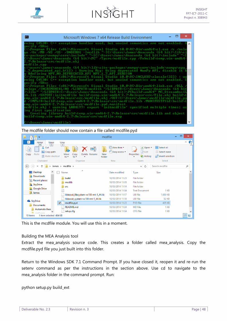
INSIGHT
FP7-ICT-2011-C
Project n. 308943
Deliverable No. 2.3 Revision n. 3 Page | 48
The mcdfile folder should now contain a file called mcdfile.pyd
This is the mcdfile module. You will use this in a moment.
Building the MEA Analysis tool
Extract the mea_analysis source code. This creates a folder called mea_analysis. Copy the
mcdfile.pyd file you just built into this folder.
Return to the Windows SDK 7.1 Command Prompt. If you have closed it, reopen it and re-run the
setenv command as per the instructions in the section above. Use cd to navigate to the
mea_analysis folder in the command prompt. Run:
python setup.py build_ext

INSIGHT
FP7-ICT-2011-C
Project n. 308943
Deliverable No. 2.3 Revision n. 3 Page | 49
This creates the spike extraction C module. You can now run python main.py To run the main
interface. You should see a window like this:
If so, you have successfully build the MEA Analysis tool. You can use it yourself by running it from
the command line. To distribute the tool to users who do not have a build environment on their PC,
return to the SDK Command Prompt and type
python setup.py bdist_msi
This creates a Windows installer file in the dist subfolder of the mea_analysis folder. Users can
install this without having to separately download any pre-requisite software.

INSIGHT
FP7-ICT-2011-C
Project n. 308943
Deliverable No. 2.3 Revision n. 3 Page | 50
Appendix C: Software Tools User Guide
If you have been given a software installer, first double click the installer file and follow the
instructions on screen.
After the install completes, you should have an icon called “MEA Analysis” on your desktop.
Double click to open the MEA Analysis software. You will see an empty screen. To get started,
choose the “Add” menu under “Processing” and select “MCD File”:
Under options, you should see a button called “Open MCD File”. Click this and select the location
of an MCD file, then click open.
If the file is large, it will take some time to load. When completed you will see a screen like this.

INSIGHT
FP7-ICT-2011-C
Project n. 308943
Deliverable No. 2.3 Revision n. 3 Page | 51
The window shows the following:
Processing (top left) – this shows a list of processing modules. At the moment you have
only one, which is the MCD File you just opened. The name of the MCD file is displayed.
When we add more modules later on, these will appear in this list.
Options (left, middle) – options for the currently selected module. In this case, you can
change the MCD file from here.
Channels (right) – here is a list of channels available in each of the loaded processing
modules.
Time selection (bottom) – you can select the time period to plot, either by clicking in the
display at the very bottom and dragging the mouse to select the time period, or by
entering the time in seconds into the “Start” and “End” inputs.
Plots (centre) – There are no plots yet. They will appear in the central region.
Adding a plot
First select some channels to plot. Click on the checkboxes next to the names of the channels.
Optionally, choose a channel group from the dropdown above the channel list before selecting a
channel to plot some of the channels in a different colour.

INSIGHT
FP7-ICT-2011-C
Project n. 308943
Deliverable No. 2.3 Revision n. 3 Page | 52
For example, above we have selected channel 12 in group A (black) and channel 13 in group B
(black).
You can click again on a channel to remove it from the plot, or click the number “1” above to select
all available channels in the processing module.
Now, from the “Plot” menu, select “Trace”.
The two channels have now been plotted in the central area. Note that only the first second has
been selected. Entering a new time selection in the input boxes, or clicking on the time display at
the bottom of the screen can alter which time period is plotted. Changes you make here will
update straight away on the plot.

INSIGHT
FP7-ICT-2011-C
Project n. 308943
Deliverable No. 2.3 Revision n. 3 Page | 53
Add multiple processing modules
In order to determine if there is any spiking activity in your data, you will need to add an “Extract
spikes” module. Select this from the “Add” menu in the “Processing” section.
After this, the options available below the module list will change to the spike extraction
parameters.
A set of defaults will be offered which you may wish to try. If noise is detected as spikes, or spikes
are detected as noise you may wish to change these later.
Notice that the “Channels” section now has two processing modules available:

INSIGHT
FP7-ICT-2011-C
Project n. 308943
Deliverable No. 2.3 Revision n. 3 Page | 54
The second column, “2”, refers to the spike extraction module. Click on the number 2 to select all
channels, then select “Raster” from the plot menu. You should see a plot like this, if not, try
selecting a different time period, or adjusting the spike extraction parameters.
To investigate how well the spike extraction is working, you can plot the spikes on the same view as
a trace. Select both data and spike extraction modules for one of the channels that shows some
spikes, then use “Trace” from the plot menu.

INSIGHT
FP7-ICT-2011-C
Project n. 308943
Deliverable No. 2.3 Revision n. 3 Page | 55
The detected spikes appear marked by “x” alongside the normal trace. Note that a spike just before
11s has not been detected here, because it falls outside the “peak within” range in the spike
extraction parameters, which currently has a lower bound of -50µV. Change this and click “apply”
to recalculate the spikes. Note that all plots will be updated, so the raster plot which is still shown
in a tab at the top of the plot view will now reflect the new spikes.
Save a plot as an image file
Right click anywhere in the plot window, and select “Save figure”.
Save calculated spikes for later analysis
Right click on the “Spikes” entry in the processing list and select “Save result”. Enter a file name
such as “spikes.npz”. Then click “Clear” and select “NPZ File” from the “Add menu”. Click the “Open
NPZ File” button and select the file you just created. Note that only the time period you have
selected will be saved in the output file. To save all the data available, you must select the entire
time period.

INSIGHT
FP7-ICT-2011-C
Project n. 308943
Deliverable No. 2.3 Revision n. 3 Page | 56
Merge multiple spike channels into a single group
After adding a data file and a spike extraction module, select “Merge spike channels” from the
“Add” menu. The “Options” area now allows you to configure some new channels. As example
configuration is loaded to begin with:
This creates two new channels, A and B, which are the combination of 12 and 13, and 22 and 23
respectively. The channels A and B appear at the bottom of the channels list on the right (you may
need to scroll down to find them). They are spike channels and so can be plotted on raster plots.

INSIGHT
FP7-ICT-2011-C
Project n. 308943
Deliverable No. 2.3 Revision n. 3 Page | 57
Appendix D: Hippocampal Slice Paper
Output: Marra, V., Burden, J.J., Crawford, F., and Staras, K. (2014). Ultrastructural readout of
functional synaptic vesicle pools in hippocampal slices based on FM-dye-labeling and
photoconversion. Nature Protocols In press. (attached as PDF file)

1
Ultrastructural readout of functional synaptic vesicle pools in hippocampal
slices based on FM-dye-labeling and photoconversion
Vincenzo Marra1,2, Jemima J. Burden3, Freya Crawford1, Kevin Staras1*
1School of Life Sciences, University of Sussex, Brighton, BN1 9QG, UK.
2Department of Cell Physiology and Pharmacology, University of Leicester, Leicester
LE1 9HN, UK. 3Medical Research Council Laboratory for Molecular Cell Biology and
Cell Biology Unit, University College London, Gower Street, London WC1E 6BT, UK.
*Correspondence: [email protected]
Key words:
presynaptic terminal; FM1-43; synaptic vesicle; hippocampus; acute slice; electron
microscopy
Running title:
Ultrastructure of native hippocampal vesicle pools
2
Fast activity-driven turnover of neurotransmitter-filled vesicles at presynaptic
terminals is a critical step in information transfer in the central nervous system.
Characterizing the relationship between the nanoscale organization of synaptic
vesicles and their functional properties during transmission is of important current
interest. Here, we outline a procedure for ultrastructural investigation of functional
vesicles in synapses from native mammalian brain tissue. FM-dye is injected into the
target region of a brain slice and upstream axons are electrically activated to
stimulate vesicle turnover. In the presence of diaminobenzidine, photo-activation of
dye-filled vesicles yields an electron-dense precipitate visible in electron micrographs.
When combined with serial-section electron microscopy, fundamental ultrastructure-
function relationships of presynaptic terminals in native circuits are revealed. We
outline the utility of this protocol for the three-dimensional reconstruction of a
recycling vesicle pool in CA3-CA1 synapses from acute hippocampal slice, and
characterization of its anatomically-defined docked pool. The protocol requires 6-7
days.

3
INTRODUCTION
In the central nervous system, fast neuron-neuron information transfer primarily
takes place at chemical synapses, specialized and ultrastructurally distinct junction
points at which presynaptic and postsynaptic structures lie closely apposed1. The
presynaptic terminal is characterized by a cluster of neurotransmitter-containing
synaptic vesicles and transmission proceeds with their activity-driven fusion leading
to the discharge of chemical transmitter towards postsynaptic receptors. While
vesicles appear morphologically equivalent they can be sub-divided into pools on the
basis of their functional behaviour, including a recycling pool (see 2,3, readily-
releasable pool4, spontaneous pool5,6 and superpool7,8. Understanding the properties
of these pools has become increasingly important with the realization that they are
potentially critical substrates in setting synaptic strength9,10 and represent modifiable
targets on which forms of plasticity9,11-15 or disease-like conditions16-18 might act to
modulate or disrupt information flow.
Labeling and visualizing functional vesicles
Extensive research has focussed on the kinetic characterization of vesicle turnover
in specific pools19 but there is also substantial interest in approaches that can link
such functional properties with information about the physical organization of
vesicles within synaptic compartments. This presents a challenge because synapses
are small with complex nanoscale morphology which is not readily resolvable using
conventional light microscopy. Elegant methods relying on nano-particles such as
quantum dots20,21 and super-resolution fluorescence imaging8 provide important
strategies to address this challenge, but are still limited in spatial information and
ultrastructural context. An alternative approach is to combine a functional measure of

4
vesicle pools with subsequent ultrastructural investigation. One of the most widely-
used methods exploits FM-dyes, fluorescent reporters that readily bind to lipid
membrane and are taken up into recycling vesicles during endocytosis to provide a
functional readout of vesicle turnover22-24. One dye variant, FM1-43, and its fixable
form FM1-43FX, also efficiently drives the polymerization of diaminobenzidine (DAB)
when photoactivated, leading to the formation of an osmiophilic precipitate25-32. In
this way, functional vesicle pools that were previously labelled with FM-dye can be
directly identified in electron micrographs. This goes substantially beyond the
information offered by fluorescence-based assessment of FM-dye signal, providing
an opportunity to assess the arrangement of recycled vesicles in the context of their
local ultrastructure; for example, with respect to defined synaptic structures (e.g. the
active zone) and other vesicle pools. An established alternative method to the use of
FM-dye staining/photoconversion relies on the labeling of endocytosing vesicles with
horseradish peroxidase (HRP) which can catalyze the conversion of DAB to an
electron-dense form. This approach has substantial merit but the efficiency of HRP
labeling of endocytosing vesicles is significantly lower than with FM-dyes, perhaps
attributable to its higher molecular weight and limited solubility32. As such its
usefulness for detailed characterization of vesicle pools is more limited.
Ultrastructural analysis based on FM-dyes has been used extensively and
highly successfully in cultured neurons7,10,25,29,31,33-36, a number of large, peripheral
terminals27-30,32,37-39, and large central release sites such as calyx of Held26 revealing
important information about organizational principles of vesicle pools. However, only
recently40 has this method been successfully applied to small central synapses in
native brain tissue, where neurons are retained in relevant circuits with defined
cytoarchitecture. This reflects the fact that the thick tissue of a brain slice presents a
5
number of technical challenges compared to, for example, cultured neurons. These
include the need to devise ways to provide good FM-dye access to the target region,
the requirement for fast fixation with excellent ultrastructural preservation, the
accurate calibration of the photoconversion reaction to achieve the correct formation
of an electron-dense precipitate, and the nanoscale relocation of the target region in
embedded tissue. The current protocol outlines an approach that addresses these
issues to allow detailed analysis of functional vesicle pools in synaptic terminals in
the stratum radiatum of CA1 in acute hippocampal slices (Fig. 1a-f). The principal
dye-labeling step is based on an established approach adopted in a number of
previous studies7,13,35,40-44 and we outline key strategies to validate its success.
Subsequently, detailed methodology for rapid microwave-enhanced fixation45 and
calibrated photoconversion of the target region are provided. Using serial-section
and three-dimensional reconstruction methods we demonstrate the utility of this
approach for characterizing a functional vesicle pool in a target synapse.
Applications and future adaptations
The protocol lends itself to an array of applications and future adaptations. Since it
makes use of a standard and widely-employed acute brain slice preparation, it can
be readily combined with conventional methodologies to provide an ultrastructural
extension to established experimental approaches; for example, electrophysiological
investigation, fluorescence imaging or pharmacological studies. Key applications
could include the investigation of presynaptic changes occurring in long-term
plasticity or in elucidating presynaptic changes in genetic mouse models. With
specific variations of the stimulation protocols, it also provides an approach to
investigate the recycling of different vesicle pools and/or endocytic mechanisms. In
6
the face of the rapid development of large-volume automated electron microscopy
approaches, a nanoscale readout of synaptic activity at the level of functional vesicle
pools is likely to become an important tool.
Experimental Design
This protocol describes an experimental procedure for the dye-labeling of functional
synapses in living brain slice, followed by steps to fix the sample and photoconvert
the fluorescence signal into an electron-dense form suitable for ultrastructural
characterization. As we outline in the step-by-step procedure, FM-dye is applied by
pressure injection into the target region of the slice and, at the same time, upstream
axons are electrically stimulated to evoke vesicle turnover. A key issue for this type
of experiment is to ensure saturating dye penetration to all areas of the region of
interest. To achieve this, dye is injected at a high concentration (20 M) at a depth
~50 m from the slice surface for an extended period before and after stimulation.
The movement of the dye through the tissue can be directly visualized by imaging
during dye-injection, and in our experiments, a high-concentration of dye readily
diffuses in the slice to occupy an approximately spherical volume extending up to the
surface. To confirm that this leads to consistent synaptic labeling across the region
of interest, we recommend performing pilot experiments after the completion of dye-
loading and washing steps to test for uniform punctate fluorescence. This can be
carried out by making comparisons of intensity measurements of fluorescent puncta
near the injection site versus those of other regions displaced laterally or in the z-
plane. For additional steps to validate the presence of functional terminals see BOX
1.
7
Another issue regarding penetration relates to the photoconversion reaction;
establishing that photoconversion product is maximally and homogeneously
distributed across the region of interest is a key requirement. A confounding factor is
that photoconversion is necessarily achieved by illumination arising from a uni-
directional light source above the sample. Thus, as the reaction proceeds, build-up
of DAB photoconversion product at the surface (nearest to the light source) gradually
occludes light penetration at greater depths, potentially limiting further
photoconversion of less superficial tissue. As outlined below (see Equipment
Setup), the measurement of transmitted light to monitor the accumulation of
photoconverted product in the sample offers a useful indicator of the progression of
the reaction. However, it is also important, particularly if the experimenter is
interested in studying synapses over different depths within the tissue, to establish
that reaction product is uniformly distributed through tissue depth at ultrastructural
level. For our system, we observe comparable levels of photoconverted vesicles
across a depth range of 2-50 ms from the top surface of the slice. As a precaution,
however, we typically target only a subset of this range (5-30 m) to ensure that we
are using the same conditions for comparison from slice to slice.
MATERIALS
REAGENTS
Diaminobenzidine (DAB; Kem-En-Tec, cat. no. 4170) ! CAUTION. May cause
genetic defects and cancer. Wear gloves and, as far as possible, work in the fume
hood.

8
DDSA (TAAB Laboratories Equipment, cat. no. DO27) ! CAUTION. Irritant to skin.
Wear gloves. All waste to be disposed of according to national hazardous chemical
regulations.
DMP-30 (TAAB Laboratories Equipment, cat. no.DO32) ! CAUTION. Harmful if
swallowed; irritant to eyes and skin. Wear gloves. All waste to be disposed of
according to national hazardous chemical regulations.
D-glucose (Sigma-Aldrich, cat. no. G8270)
Dimethyl sulfoxide (Sigma-Aldrich, cat. No. 472301)
FM1-43FX (Invitrogen, cat. no. F-35355)
Glutaraldehyde 25% solution (Agar Scientific, cat. no. AGR1312) ! CAUTION. Toxic
by inhalation; corrosive; harmful if swallowed; irritant by inhalation and skin contact;
dangerous to the environment. Wear gloves and work in the fume hood. All waste to
be disposed of according to national hazardous chemical regulations.
Glycine (Sigma-Aldrich, cat. no. G8898)
Magnesium chloride (Sigma-Aldrich, cat. no. M8266)
MNA (TAAB Laboratories Equipment, cat. no. MO11) ! CAUTION
Osmium tetroxide (TAAB Laboratories Equipment, cat. no. O021) ! CAUTION. Toxic
by inhalation, in contact with skin and if swallowed. Keep stored in a double
container in a dangerous chemicals fridge. Wear gloves and work in the fume hood.
All sample incubations need to also be placed in a sealable Tupperware container
dedicated for use with osmium tetroxide. All waste to be disposed of according to
national hazardous chemical regulations.
Formaldehyde 16% solution (Agar Scientific, cat. no. AGR1026) ! CAUTION.
Harmful by inhalation, in contact with skin and if swallowed; irritant to eyes

9
respiratory system and skin. Wear gloves and work in the fume hood. All waste to be
disposed of according to national hazardous chemical regulations.
Potassium chloride (Sigma-Aldrich, cat. no. P9333)
Potassium ferrocyanide (Sigma-Aldrich, cat. no. 455989) ! CAUTION. Harmful by
inhalation, in contact with skin and if swallowed; irritant to eyes. Wear gloves and
work in the fume hood. All waste to be disposed of according to national hazardous
chemical regulations.
Propylene oxide (Agar Scientific, cat. no. AGR1080) ! CAUTION. Toxic, may cause
cancer and heritable genetic damage; harmful by inhalation, in contact with skin and
if swallowed; irritant to eyes respiratory system and skin; extremely flammable.
Corrodes some plastics, so use glass pasteurs and glass dishes or vials for
incubations. Wear latex gloves and work in the fume hood. All waste to be disposed
of according to national hazardous chemical regulations.
Sodium cacodylate (Agar Scientific, cat. no. AGR1104) ! CAUTION. Toxic, may
cause harm to the unborn child; harmful by inhalation, in contact with skin and if
swallowed; irritant to eyes. Wear gloves and work in the fume hood. All waste to be
disposed of according to national hazardous chemical regulations.
Sodium chloride (Sigma-Aldrich, cat. no. 746398)
Sodium hydrogencarbonate (Sigma-Aldrich, cat. no. 401676)
Sodium phosphate monobasic (Sigma-Aldrich, cat. no. S9638)
TAAB 812 (TAAB Laboratories Equipment, cat. no. TO23) ! CAUTION. Irritant to
eyes and skin; dangerous to the environment. Wear gloves and work in the fume
hood. All waste to be disposed of according to national hazardous chemical
regulations.

10
Uranyl acetate (Agar Scientific, cat. no. AGR1260A) ! CAUTION. Very toxic by
inhalation and if swallowed; dangerous for the environment. Wear gloves and work in
the fume hood. All waste to be disposed of according to national hazardous chemical
regulations.
Hippocampal slices of interest. In this protocol we describe the use of acute
transverse hippocampal slices (300 µm thickness) from 21-28 day rats. For further
information about preparing hippocampal slices see refs46,47. ! CAUTION All animal
experiments must comply with national regulations. CRITICAL Place slices into
aCSF bubbled with 95% O2 and 5% CO2 (Carbogen) immediately.
EQUIPMENT
Anti-vibration table (e.g. 780 series, TMC)
Amplifier (e.g. Multiclamp 700B, Molecular Devices)
A-D converter (e.g. Digidata 1550, Molecular Devices)
CCD camera (e.g. QIClick, Q-Imaging)
Confocal microscope equipped with Argon laser; upright microscope (e.g. Olympus
model: BX51WI or comparable) with confocal head (Olympus, model: Fluoview
FV300 or comparable) and x4 (PLN4X), x40 (LUMPLFLN40XW), x60
(LUMPLFLN60XW) objectives.
Embedding capsules (Agar Scientific, cat. no. G360-1,00 BEEM capsules)
Formvar-coated slot grids (TAAB Laboratories Equipment, cat. no. F218/050)
Grid Box (e.g. Gilder SB50, TAAB Laboratories Equipment)
Hg epifluorescence lamp for photoconversion (Omega Optical XF100-2, Dichroic
mirror 500 nm to direct light for photoconversion)
Illumination for stereomicroscope (e.g. KL 1500 LCD, Schott UK)

11
Micromanipulator (LBM or equivalent, Scientifica)
Microwave oven (e.g. Panasonic NN-E289M) CRITICAL Only required if using
microwave fixation (Box 2)
Peristaltic pump (e.g. Minipuls 3, Gilson)
Pipette puller (e.g. PC-10, Narishige)
Platinum wire 0.5 mm thick (Alfa Aesar, cat. no. 10286)
Pressure injection system (e.g. Picospritzer, Parker)
Stimulator (e.g. Grass SD-9)
Stereomicroscope (e.g. Stemi 2000, Carl Zeiss)
Thermometer (e.g. RS Components, 615-8212)
Theta glass CG200T (Harvard Apparatus Ltd, cat. no. 300117)
Tungsten wire 0.075 mm thick (Alfa Aesar, cat. no. 00457)
Ultramicrotome (e.g. EM UC7, Leica)
Vibrating microtome (e.g. VT1200S, Leica)
REAGENT SETUP
Artificial cerebrospinal fluid (aCSF) Prepare solution containing: 125 mM NaCl,
2.5 mM KCl, 25 mM glucose, 1.25 mM NaH2PO4, 26 mM, NaHCO3, 1 mM MgCl2, 2
mM CaCl2, 50 M AP5 saturated with gaseous mixture of Carbogen (95% O2 and 5%
CO2)(pH 7.3). Prepare fresh solution on the first day of the experimental protocol.
Fixative On the first day of the experimental protocol prepare a solution containing 1
ml of 10x PBS, 1.25 ml of 16% Formaldehyde, 2.4 ml Glutaraldehyde and bring to 10
ml volume using ddH2O. This produces a solution with final concentrations of 6%
glutaraldehyde, 2% formaldehyde with pH 7.3. ! CAUTION. Harmful by inhalation, in
contact with skin and if swallowed; irritant to eyes respiratory system and skin. Wear

12
gloves and work in the fume hood. All waste to be disposed of according to national
hazardous chemical regulations.
DAB Add one tablet of Diaminobenzidine-PBS (Kem-En-Tec, cat. no. 4170) to 10 ml
of ddH2O and sonicate for 10 minutes. Prepare fresh immediately before use and
minimise exposure to light. ! CAUTION Diaminobenzidine may cause genetic defects
and cancer. Avoid contact with skin. After use, place all contaminated plastic and
glassware in bleach for 48 h. Handle objective lens with gloves and rinse extensively
with ddH2O after use.
EPON solution In a disposable beaker on a measuring scale add 24g of TAAB 812,
9.5g of DDSA, 16.5g MNA and finally 1g of DMP30, vortex the solution for 1 min and
wait ~5 mins for air bubbles to surface. Prepare fresh on the day of use, and allow 30
mins for it to mix thoroughly. ! CAUTION Reagents can be irritant to eyes and skin
and dangerous to the environment. Wear gloves and work in the fume hood. All
waste to be disposed of according to national hazardous chemical regulations.
FM1-43FX solution 10 mM FM1-43FX stocks should be kept at -20ºC in DMSO;
they can be stored for up to 3 months. On day of experiment, make 500 ls of 20 M
FM-dye solution by diluting the stock in bubbled aCSF.
Sodium cacodylate buffer 0.1M sodium cacodylate in ddH2O adjusted to pH 7.4
with HCl. The solution can be stored at 4ºC for 3 months. ! CAUTION Sodium
cacodylate is toxic and harmful by inhalation, in contact with skin and if swallowed;
irritant to eyes. Wear gloves and work in the fume hood. All waste to be disposed of
according to national hazardous chemical regulations.
Uranyl acetate solution Prepare 4% uranyl acetate in 70% ethanol fresh on the
second day of the experimental protocol. Vortex the solution for at least 5 minutes
and filter immediately before use. ! CAUTION. Uranyl acetate is very toxic by

13
inhalation and if swallowed; dangerous for the environment. Wear gloves and work in
the fume hood. All waste to be disposed of according to national hazardous chemical
regulations.
EQUIPMENT SETUP
Bipolar tungsten stimulating electrode A number of bipolar stimulating electrodes
are commercially available (Metal microelectrode, WPI). Alternatively, stimulating
electrodes can be fabricated by inserting one tungsten wire 0.075 mm thick (Alfa
Aesar, cat. no. 00457) in each of the two compartments of a theta glass capillary
(Harvard Apparatus Ltd, cat. no. 300117). Pull the capillary over the blue flame of a
Bunsen burner to produce an electrode with a fine tip (~0.2 mm). Each tungsten wire
is soldered at one end to a suitable electric wire for connection to the stimulator (e.g.
SD-9, Grass stimulator)(Fig. 2a)
U-shaped harp-slice grid Harps can be purchased (e.g. Harvard Apparatus, cat. no.
64-0254) or manufactured by bending a segment of platinum wire (Alfa Aesar, cat.
no. 10286) in a U-shape (0.5 mm in diameter and ~25 mm in length); the two arms of
the U should be at least 6 mm apart. The wire is then flattened using a bench-top jaw
drill press and 4-6 nylon threads are attached with cyanoacrylate glue between the
two arms of the U-shaped wire with spacing of 1.5-2 mm (Fig. 2b).
Glass O-ring Using cyanoacrylate glue, attach 4-6 nylon threads onto one side of a
glass ring (internal diameter 15 mm and 5 mm thick).
Pressure injection system Connect the pressure outlet of the pressure injection
system (e.g. Picospritzer, Parker) to the ‘pressure’ port of a patch-clamp electrode

14
holder (e.g. Series Q holders, Harvard Apparatus Ltd) which is also connected to
your amplifier.
Electrophysiological Recording setup Set up following manufacturer’s instructions.
Further details and useful advice on how to set up an electrophysiology rig can be
found in the Axon Guide
http://mdc.custhelp.com/euf/assets/content/Axon%20Guide%203rd%20edition.pdf
Imaging setup Follow the manufacturer’s instruction to set up the imaging system.
Select a suitable excitation wavelength to visualize FM1-43FX (i.e. 488 nm with
confocal, 840 nm with multiphoton laser). The emission range for FM1-43FX is broad
with a peak at 580 nm; select suitable emission filter for visualization (e.g. BP530/30
or BP590/34).
Microwave fixation calibration If the preferred method of fixation relies on
microwave fixation, this procedure will require calibration steps prior to the start of an
experiment (see BOX 2).
PROCEDURE
FM-dye labeling and fluorescence imaging (3-4 hours)
1. Place the acute transverse hippocampal slices (300 m thickness)46,47 in aCSF
bubbled with 95% O2 and 5% CO2 (Carbogen). Allow slices to recover for 30 mins at
37º C followed by 30 mins at room temperature (20º C).
2. Using a transfer pipette, move a slice from the recovery chamber to the imaging
chamber containing bubbled aCSF, continuously perfused at a rate of 2-5 mls/min.

15
3. Place harp-slice grid on top of the slice to anchor the tissue and allow the slice to
equilibrate for 15 mins.
4. Place tungsten stimulating electrode on stratum radiatum to stimulate Schaffer
collaterals (Figs. 1a, 3a).
5. Place a recording electrode containing aCSF and 20 M FM1-43FX in the stratum
radiatum of CA1 region (Fig. 3a). The tip of the electrode should be ~50 m below
the surface of the slice.
6. Stimulate at 0.2 Hz (0.8-1 ms) using a voltage between 0.1 and 2V; each tungsten
electrode will need to be calibrated separately. The objective of this step is to obtain
a repeatedly-evoked field excitatory post-synaptic potential (fEPSP) with an
amplitude of at least 0.2 mV (Fig. 3b).
7. Once a robust postsynaptic response is achieved, change the perfused solution to
aCSF+20 M CNQX to reduce recurrent excitation of the network.
8. Using the pressure injection system, provide 15-20 psi positive pressure to the
recording electrode to locally apply FM-dye for 7 mins. 3 mins after the start of this
dye-application step begin 10 Hz stimulation through stimulating electrode for 2 mins
using the voltage settings determined in step 6. The period of dye application after
the end of the stimulation is necessary to allow complete uptake of FM-dye during
endocytosis.
9. Carefully remove recording electrode from slice chamber and leave the slice for
10-20 mins with continuous perfusion of aCSF+CNQX to wash residual FM-dye from
extracellular membranes. This washing step may benefit from the use of chemical
agents (e.g. Sulforhodamine39 or Advasep-746) that can help to improve the
visualization of vesicular FM-dye

16
10. Perform confocal fluorescence imaging of CA1 region and establish presence of
FM-dye-labelled synaptic terminals. These should appear as discrete fluorescent
puncta at depths starting from 2-5 m from the top of the slice (Fig. 3c). For steps to
confirm the functionality of these synapses see Fig. 4a-c and BOX 1.
? TROUBLESHOOTING
11. Using CCD camera, take x60 and x4 magnification brightfield images of target
region to assist with its re-location in step 17.
Fixation and photoconversion of sample (100-120 min)
12. Remove the stimulating electrode and harp-slice grid and using a transfer pipette
move the slice to a plastic petri-dish containing freshly-bubbled aCSF+CNQX.
Ensure that the slice is correctly orientated in the dish (same side up) and place
glass O-ring on slice to anchor tissue.
13. Transfer petri-dish to fume hood for fixation.
14. Fix tissue. For a discussion of optimal approaches to fix thick brain tissue we
refer the reader to 45. The established method we use relies on microwave fixation,
using a calibrated microwave, and is described in BOX 2.
? TROUBLESHOOTING
15. Replace fixative with 100 mM glycine in PBS and leave for 1 hr.
16. Rinse in 100 mM NH4Cl (1 min) and rinse well with fresh PBS.
17. Transfer chamber back to imaging rig and relocate target region using the
brightfield image(s) collected in step 11.

17
18. Raise objective and replace extracellular solution with carbogen-bubbled
diaminobenzidine solution (DAB, 1 mg/ml). Leave to incubate for 10 mins. !
CAUTION Diaminobenzidine may cause genetic defects and cancer. Avoid contact
with skin. After use, place all contaminated plastic and glassware in bleach for 48 h.
Handle objective lens with gloves and rinse extensively with ddH2O after use.
19. Replace with fresh DAB solution and continue to bubble with carbogen. Lower
objective and focus on the top of the slice in the target region. Note that a dedicated
objective is required for DAB photoconversion steps (e.g. 40x, NA 0.8 water
immersion objective, objective power density: ~1500 mW/cm2). ! CAUTION See step
18.
20. Illuminate region of interest with intense blue light (<500 nm from a 100 W
Mercury lamp) for 15-25 mins (e.g. Olympus UMNB-2 with excitation filter removed).
The objective here is to irradiate the slice with a wavelength that maximally excites
across the peak absorption wavelengths of FM-dye (see Fig 5a-c and BOX 3 for
calibration of photoconversion reaction). With the appropriate steps, the
photoconverted region is clearly identifiable as a dark area in the slice (Fig. 5c). !
CAUTION See step 18.
? TROUBLESHOOTING
21. Replace DAB solution with PBS and wash a further three times with fresh PBS
solution to ensure removal of DAB. Collect brightfield images of the photoconverted
region in the tissue. This is necessary to ensure precise relocation of the target
region with respect to the rest of the slice structure, following embedding.

18
22. Transfer sample to fume hood. Replace PBS with 0.1M sodium cacodylate buffer
and wash a further three times. This is to ensure that phosphate groups have been
removed. ! CAUTION Perform steps 22-36 in a fume hood. Sodium cacodylate is
toxic and harmful by inhalation, in contact with skin and if swallowed; irritant to eyes.
Wear gloves and work in the fume hood. All waste to be disposed of according to
national hazardous chemical regulations.
PAUSE POINT Samples can be stored at 4oC overnight.
Sample embedding (~90 hrs)
23. Replace 0.1M sodium cacodylate buffer with 1.5% potassium ferrocyanide / 1%
osmium tetroxide in 0.1M sodium cacodylate buffer for 1 hr. ! CAUTION See step 22.
24. Wash thoroughly in cacodylate buffer (5 x 10 mins). ! CAUTION See step 22.
25. Replace with 1% osmium tetroxide in 0.1M sodium cacodylate buffer for 1 hr. !
CAUTION Osmium tetroxide is toxic by inhalation, in contact with skin and if
swallowed. Keep stored in a double container in a dangerous chemicals fridge. Wear
gloves and work in the fume hood. All sample incubations need to also be placed in
a sealable Tupperware container dedicated for use with osmium tetroxide. All waste
to be disposed of according to national hazardous chemical regulations. Also see
step 22. ! CRITICAL STEP Osmium tetroxide is used in multiple steps to maximise
the contrast within the block and therefore avoid the need for additional staining on
the sections. Hence, the double osmium tetroxide and the en bloc uranyl acetate
steps.

19
26. Wash thoroughly in cacodylate buffer until all traces of the osmium fixative have
been removed. ! CAUTION See step 22.
PAUSE POINT Samples can be stored at 4oC overnight.
27. Replace cacodylate buffer with 50% ethanol for 10 mins. ! CAUTION See step 22.
28. Stain en bloc with 4% uranyl acetate in 70% ethanol for 1 hr. ! CAUTION Uranyl
acetate is very toxic by inhalation and if swallowed; dangerous for the environment.
Wear gloves and work in the fume hood. All waste to be disposed of according to
national hazardous chemical regulations.
29. Prepare EPON solution as described in REAGENT SETUP. Prepare a 1:1
EPON:propylene oxide mixture in a glass vial and vortex thoroughly.
!CAUTION Store all solutions in the fume hood.
30. Dehydrate in ethanol stepwise (2 x 75%, 2 x 90%, 2 x 100%, 5 mins each).
31. Using blunt forceps transfer the samples to a glass petri dish containing 1:1
propylene oxide:EPON. Take care as sample will be brittle. Ensure the samples are
completely immersed in the mixture. Cover and leave overnight in fume hood.
PAUSE POINT Samples are stored overnight in fume hood.
32. Prepare fresh EPON solution as described in REAGENT SETUP and carefully
replace propylene oxide:EPON mix with 100% EPON. Replace with fresh EPON
after 12 hrs and leave for a further 12 hrs.
33. Detach the lid of a BEEM capsule, and use a razor blade to remove the conical
end (Fig. 6a).

20
34. Using blunt forceps transfer the samples into BEEM capsule lids ensuring the
photo-illuminated face of the slice is facing downwards (Fig. 6b). Each sample
needs to be in the centre of a separate lid.
35. With the lid resting on a flat surface, insert the BEEM capsule cylinder (Fig. 6c).
36. Carefully fill the capsule with EPON from the open end ensuring that the EPON
is applied above the sample to minimize lateral movement of the tissue (Fig. 6c).
37. Place capsules in an oven at 60oC for 48 hrs to polymerize EPON.
38. Remove and store carefully at room temperature.
PAUSE POINT. The sample can be stored for an extended period at room
temperature (months to years).
Sectioning, electron microscopy and reconstruction (10-14 hrs)
39. Carefully remove the BEEM capsule plastic surrounding the polymerize EPON
using a razor blade. The tissue should appear very dark, approximately central in the
cylinder and flat to the surface of the capsule (Fig. 6d,e).
40. Using a stereomicroscope identify the target photoconverted region. This can be
readily achieved using local structural landmarks by aligning the pre-embedding
brightfield images of the tissue (see step 21) with images of the embedded tissue
(Fig. 6f,g). Alternatively, by altering the incidence angle of brightfield illumination the
photoconverted region can be visualized by its different light-scattering properties
(Fig. 6g, inset). Mark the region by lightly scoring it with a scalpel blade.
41. Asymmetrically trim block up to scalpel marks. Using an ultramicrotome, cut
silver/gold (60–70 nm thickness) serial sections. Assuming the sample is flat and

21
precisely parallel to the sectioning face, we recommend to collect ribbons of serial
sections over a range of 2-30 ms from the top of the slice. 2 ms represents the
minimal tissue depth below the superficial cut surface of the slice, where there is the
likelihood for intact axons and photoconverted vesicles.
42. Collect continuous ribbons of serial sections on 1 mm x 2 mm Formvar-coated
slot grids.
43. Air dry grids for 15 min and store in grid box.
PAUSE POINT The grids can be stored for several months at room temperature
44. View sections using an electron microscope fitted with a cooled CCD camera
(Fig. 7a). Acquire images of synapses and use local landmarks to identify the same
target synapse in consecutive sections to facilitate a serial reconstruction.
? TROUBLESHOOTING
45. Classify vesicles as photoconverted (PC+) or non-photoconverted (PC-). PC+
vesicles have a characteristically electron-dense lumen compared to the clear lumen
of non-recycling vesicles (Fig. 7b,c). Most vesicles can be readily categorized by
visual assessment. However, there are also a number of established quantitative
approaches to aid in vesicle classification based on comparisons of membrane and
lumenal optical densities25,30,31,33.
46. Use reconstruction software such as ‘Reconstruct’
(http://synapses.clm.utexas.edu/tools/reconstruct/reconstruct.stm) or ‘Fiji’
(http://fiji.sc/Fiji) to align images and build a cartoon representation of a target
synapse of interest (Fig. 7d). These software packages provide clear and
comprehensive guidance for reconstruction approaches in online manuals (e.g.

22
http://synapses.clm.utexas.edu/tools/reconstruct/ReconstructUserManualv1.1.0.0.pdf)
and video tutorials (e.g. http://fiji.sc/TrakEM2_tutorials).

23
BOX 1. Establishing the presence of functional FM-dye-labelled terminals.
This validation protocol is helpful in establishing that the punctate staining observed
in step 10 corresponds to functional dye-labelled presynaptic terminals. Since the
successful completion of this procedure results in the loss of synaptic dye-labeling it
is not compatible with further steps leading to the ultrastructural visualization of
functional vesicles. The rationale for this validation step is the idea that functional
synaptic labeling can be confirmed by observing a robust activity-evoked
fluorescence decrease at terminals (‘destaining’) as FM-dye-labelled vesicles
undergo fusion and dye-loss (Fig. 4a,b).
1. Carry out imaging in CA1 region and identify punctate staining as in step 10.
2. Set up a time-lapse imaging experiment with an acquisition rate of 0.5-1 Hz.
Establish a baseline of 10 frames and then begin electrical stimulation (2-20 Hz for
1200 pulses with parameter settings used for loading) while continuing to image at
the same frequency.
3. In offline analysis, measure fluorescence intensities over time in regions of interest
containing fluorescence puncta. Plots should appear as a stable baseline period
followed by a decline in fluorescence that can be described by a single exponential
decay profile. The time constant of dye-loss should be inversely proportional to the
stimulation frequency (Fig. 4c).

24
BOX 2. Using microwave-enhanced fixation.
Microwave-enhanced fixation provides a means to achieve rapid fixation of thick
tissue with excellent ultrastructural preservation45. The overall objective is to heat the
brain slice for 8-15 s to 45-50oC while immersed in fixative. This can be achieved
using a specialized microwave-based processing system or an inexpensive domestic
microwave oven placed in a fume hood. Regardless of the system chosen, the
intensity and duration of microwave irradiation needs to be initially calibrated. A
suggested protocol for a domestic microwave is outlined below.
Calibration
1. Remove the microwave plate and cover the central rotating mechanism with an
inverted petri-dish to create a stationary central platform.
2. Place a beaker containing 200 mls of ddH2O at room temperature in one of the
two rear corners of the microwave oven. Set the power of the microwave oven to 700
W and irradiate until the temperature of the water in the beaker reaches 40-45ºC.
This can be determined by immediately removing the beaker after irradiation and
measuring the temperature using a fast-read temperature probe (e.g. RS 55II
thermometer, RS Components 615-8212). The water in the beaker will absorb
reflected irradiation, improving the uniformity of irradiation of the sample.
3. With the pre-heated beaker in the rear corner, place 4 mls of fixative in a petri-dish
warmed to 37ºC on the central platform. Irradiate for 10 s and measure the
temperature of the fixative immediately after irradiation (the use of a dedicated
temperature probe is highly recommended). The final temperature of the fixative
should be 45-50ºC. If this temperature is not achieved, repeat the process using a
new fixative sample, adjusting the irradiation time accordingly. Once parameters are

25
established to meet target temperature, repeat with multiple samples to ensure
consistency.
Sample fixation
4. Prepare the microwave as in calibration step 1 above. As in step 2, place a beaker
containing 200 mls of reverse osmosis water at room temperature in the rear corner
of the microwave oven floor. Irradiate at 700 W for the time determined in step 2.
5. Rapidly place a tissue sample in a petri dish containing fixative (6%
glutaraldehyde, 2% formaldehyde in PBS at 370C) and anchor it using a glass O-ring.
Place the petri dish in the center of the microwave oven and irradiate at 700 W for
the time determined in step 3.

26
BOX 3. Monitoring the photoconversion reaction.
Accurate determination of the time necessary to photo-polymerize diaminobenzidine
(DAB) in the presence of FM1-43FX is a critical requirement for this protocol. A
number of parameters including the objective used for the photoconversion step, the
specific wavelength and power of the excitation light and the depth of the target
region within the tissue, are factors that influence the length of this process. It is
strongly recommended that initially, pilot experiments are carried out to establish this
time precisely for a given imaging system. For the actual photoconversion of
samples, we suggest proceeding in photoillumination periods of 3-5 mins. After each
period, take an image with a CCD camera of the transmitted brightfield light (Fig. 5a).
As the photoconversion reaction develops, the target region should become darker
as transmission light is reduced and this can be quantified and plotted (Fig. 5a-c).
An approximate rule of thumb is to photoconvert for an additional 5 mins after the
decline in transmitted signal has reached a steady state.

27
TIMING
Day 1, steps 1-22, 5-8 hours depending on the samples
Day 2, steps 23-31, 18 hours
Day 3, steps 32, 24 hours
Day 4, steps 33-38, 49 hours
Day 6, steps 39-43, 6 hours depending on the samples
Day 7, steps 44-46, 8 hours depending on the samples

28
? TROUBLESHOOTING
See Table 1 for troubleshooting guidance.
Table 1: troubleshooting.
Step Problem Possible Reason Solution
10 No punctate staining visible
Poor health of slice Visually assess the health of the slice. At low magnifications unhealthy slices have a fuzzy, low-contrast appearance with poor definition between anatomically-defined layers. By contrast, in stratum radiatum of a healthy slice, tissue has a more-defined and striated appearance. At higher magnifications, visually assess the health of the pyramidal neuron cell bodies in the most superficial part of the slice. They should appear densely packed and intact with smooth membranes. Use a different slice if cell health appears sub-optimal.
Sub-optimal stimulation
Repeat step 6 until a better fEPSP is evoked.
Plane of focus too deep or too superficial
Perform z-stack imaging of the x-y region of interest using large z-
steps (2-4 m) over a large z-
range (50 m) to identify depth with good staining.
Too much background signal relative to punctate staining, even with a strong stimulation loading protocol.
Extend the wash-out period to reduce non-specific staining; optimize imaging conditions (e.g. slower scan speed, increase laser power, zoom in)
14 Poor preservation of the tissue
Microwave irradiation too short or too long
Recalibrate microwave irradiation system as described in BOX 2
20 No photoconverted region identifiable
Photoillumination too brief
Size and chromaticity of the photoconverted region can vary, however a darkening of the photoilluminated region should always be observed; repeat

29
procedure to follow the photoconversion reaction described in BOX 3
Inefficient carbogen bubbling
Reduce the bore of the carbogen outlet; ensure bubble size does not exceed 2-3 mm
20
Photoconverted region has variable appearance between experiments
Photoillumination not stable
Mercury burners are not necessarily stable in their power output across their burn history. For your system, calibrate the irradiation power when photoconversion is optimal and ensure that this power is maintained for all subsequent experiments. Change the bulb if power output begins to reduce. Alternatively, test whether an alternative light source (e.g. an LED-based system), which has more stable output over its lifetime, is effective for your needs.
44 Electron-dense debris
Sections contain only the most superficial part of the sample
Use samples collected deeper in the embedded sample.
44 No photoconverted vesicles
Sections are taken from too deep below the surface of the slice.
The penetration of photoconversion reaction is limited to relatively superficial depths in the slice (up to ~50
ms). Use samples collected at sites closer to the tissue surface.

30
Anticipated Results
Figure 7 provides an overview of typical results. Within the target region (Fig. 7a),
presynaptic terminals with PC+ vesicles can be readily identified (Fig. 7b). The
characteristic electron-dense profile of such vesicles contrasts with PC- vesicles
characterized by a clear lumen (Fig. 7c). Three-dimensional reconstruction based on
consecutive serial sections provides a representation of the organization of a
recycled vesicle pool in the context of the non-recycled pool as well as other
ultrastructural features such as the active zone (Fig. 7d). This offers substantial
scope for exploring details of ultrastructure-function relationships. Here, we briefly
demonstrate one possible application: characterizing the PC+ and PC- composition
and position of vesicles comprising the anatomically-defined docked pool at the
active zone (Fig. 7e).

31
Figure Legends
Figure 1. Overview of experimental protocol. (a) Schematic showing approach for
fixable FM-dye labeling of terminals in stratum radiatum of acute hippocampal slice.
A bipolar stimulating electrode is placed on Schaffer collaterals and an FM-dye-filled
pipette positioned in CA1. DG, dentate gyrus. Dye is pressure ejected while
stimulation (1200 APs, 10 Hz) is applied. (b) Labelled terminals are photoilluminated
with blue light in the presence of diaminobenzidine (DAB). (c) After photoconversion,
synapses appear dark owing to the formation of osmiophilic precipitate in dye-filled
recycling vesicles. (d) Target region is embedded in resin and serially sectioned. (e)
In electron micrographs, presynaptic terminals contain photoconverted (PC+)
vesicles with dark lumen and non-photoconverted (PC-) vesicles. (f) 3-d models of
synaptic terminals can be constructed from serial sections. Parts of this figure have
been adapted from Marra et al.40
Figure 2. Schematics of key equipment items. (a) Bipolar stimulating electrode.
Heat-drawn theta glass contains tungsten wire in each barrel. Tip end is fire-polished
to seal around each tungsten wire. The other end of each wire is glued securely onto
a small mounting plate and soldered to plugs. (b) Harp-slice grid made from flattened
platinum wire bent to a U-shape. Nylon threads are stretched across this frame and
secured with cyanoacrylate glue.
Figure 3. Labeling functional synapses in acute slice. (a) Example brightfield
image of slice with approximate placement of stimulation and recording electrodes.

32
Scale bar, 200 m. DG, dentate gyrus. (b) Typical example of field excitatory
postsynaptic potential recordings (gray lines) from CA1 region triggered by Schaffer
collateral stimulation (stimulus 1 ms). Average trace is shown in red. Vertical line
shows end of stimulus artefact. Scale bars, 0.5 mV (vertical), 2 ms (horizontal). (c)
Typical sample image of FM dye-positive fluorescent puncta in CA1 (white arrows).
Scale bar, 1 m. Parts of this figure have been adapted from Marra et al40 and
Ratnayaka et al.35. Experiments were performed in accordance with the UK-Animal
(Scientific Procedures) Act 1986 and complied with local institutional regulations.
Figure 4. Testing activity-dependence of synaptic labeling. (a) Cartoon
illustrating the rationale for experiment to determine functional integrity in dye-filled
puncta. Fluorescence signal in synapses related to recycling vesicles (2,3) should be
lost when terminals are subjected to further stimulation (4). (b) Example frames from
timelapse sequences illustrating stimulation-frequency dependence of FM-dye-loss.
Scale bar, 1 m. (c) Dye-loss profiles for sample destaining protocols (from b). X-
axis shows time (in seconds) with respect to the onset of stimulation. Y-axis shows
fluorescence normalized to the mean of the three values immediately preceding
stimulation onset. Time constant of dye-loss, described by single exponential fits, is
inversely proportional to stimulation frequency. Experiments were performed in
accordance with the UK-Animal (Scientific Procedures) Act 1986 and complied with
local institutional regulations.
Figure 5. Monitoring progress of photoconversion. (a) Development of
photoconversion product can be followed by measuring the level of transmitted light

33
in target region (top, red square). Scale bar, 500 m. (bottom) Sample images
showing photoconversion reaction in ROI with time. Scale bar, 50 m. (b) Mean +-
SEM line plot showing reduced bright-field light transmission as photoconversion
reaction progresses. (c) Image showing appearance of target region after 20 min
photoconversion. Scale bar, 100 m. Parts of this figure have been adapted from
Marra et al.40. Experiments were performed in accordance with the UK-Animal
(Scientific Procedures) Act 1986 and complied with local institutional regulations.
Figure 6. Approach for embedding tissue in EPON. (a) Prepare BEEM capsule by
detaching lid and removing conical end with razor blade. (b) Transfer inverted slice
into lid with photoconverted side facing down. Scale bar, 2 mm. (c) Insert BEEM
capsule cylinder into lid and fill with EPON from open end, ensuring it is applied
directly above the sample (white circle). Scale bar, 2 mm. (d,e) Side (d) and half-
face (e) appearance of polymerized EPON block with embedded tissue at surface.
Scale bar, 2 mm. (f,g) Appearance of tissue immediately after fixation with
photoconverted region (f) and the same tissue after embedding in EPON (g). Inset
illustrates how the target photoconverted region is visible in EPON if light settings
are adjusted. Scale bar, 500 m. Experiments were performed in accordance with
the UK-Animal (Scientific Procedures) Act 1986 and complied with local institutional
regulations.
Figure 7. Ultrastructural readout of functional vesicles. (a) Low magnification
electron micrograph showing appearance of slice in ultrastructure. Scale bar, 2 m.
(b) Sample images of photoconverted vesicles in presynaptic terminals. Scale bar,

34
100 nm. (c) Density profiles of photoconverted vesicle (left panels) and non-
photoconverted vesicle (right panels). Scale bar, 10 nm. (d) Example reconstruction
based on 11 consecutive sections showing photoconverted and non-photoconverted
vesicles. Scale bar, 100 nm. (e) Detail on vesicle composition at active zone (green).
Scale bar, 100 nm. Experiments were performed in accordance with the UK-Animal
(Scientific Procedures) Act 1986 and complied with local institutional regulations.

35
Author contribution statements
K.S. and V.M. conceived the method and wrote the paper. F.C. validated key steps
and provided some of the figures. J.J.B. helped develop sample processing methods
and carried out serial sectioning.
Acknowledgments
This work was supported by Wellcome Trust (WT084357MF), BBSRC
(BB/K019015/1), MRC (MR/K004999/1) and EU-FP7 (308943) grants to K.S.
Competing financial interests
The authors declare that they have no competing financial interests.

36
REFERENCES
1. Sudhof, T.C. The synaptic vesicle cycle. Annu Rev Neurosci 27, 509-547
(2004).
2. Alabi, A.A. et al. Synaptic vesicle pools and dynamics. Cold Spring Harb
Perspect Biol 4, a013680 (2012).
3. Rizzoli, S.O. et al. Synaptic vesicle pools. Nat Rev Neurosci 6, 57-69 (2005).
4. Rosenmund, C. et al. Definition of the readily releasable pool of vesicles at
hippocampal synapses. Neuron 16, 1197-1207 (1996).
5. Fredj, N.B. et al. A resting pool of vesicles is responsible for spontaneous
vesicle fusion at the synapse. Nat Neurosci 12, 751-758 (2009).
6. Sara, Y. et al. An isolated pool of vesicles recycles at rest and drives
spontaneous neurotransmission. Neuron 45, 563-573 (2005).
7. Staras, K. et al. A vesicle superpool spans multiple presynaptic terminals in
hippocampal neurons. Neuron 66, 37-44 (2010).
8. Westphal, V. et al. Video-rate far-field optical nanoscopy dissects synaptic
vesicle movement. Science 320, 246-249 (2008).
9. Kim, S.H. et al. CDK5 serves as a major control point in neurotransmitter
release. Neuron 67, 797-809 (2010).
10. Ratnayaka, A. et al. Recruitment of resting vesicles into recycling pools
supports NMDA-receptor dependent synaptic potentiation in cultured hippocampal
neurons. J Physiol 590, 1585-1597 (2012).
11. Murthy, V.N. et al. Inactivity produces increases in neurotransmitter release
and synapse size. Neuron 32, 673-682 (2001).
12. Thiagarajan, T.C. et al. Adaptation to synaptic inactivity in hippocampal
neurons. Neuron 47, 725-737 (2005).

37
13. Tyler, W.J. et al. BDNF increases release probability and the size of a rapidly
recycling vesicle pool within rat hippocampal excitatory synapses. J Physiol 574,
787-803 (2006).
14. Staras, K. Share and share alike: trading of presynaptic elements between
central synapses. Trends Neurosci 30, 292-298 (2007).
15. Staras, K. et al. Sharing vesicles between central presynaptic terminals:
implications for synaptic function. Front Synaptic Neurosci 2, 20 (2010). doi:
10.3389/fnsyn.2010.00020
16. Murphy, D.D. et al. Synucleins are developmentally expressed, and alpha-
synuclein regulates the size of the presynaptic vesicular pool in primary hippocampal
neurons. J Neurosci 20, 3214-3220 (2000).
17. Scott, D. et al. alpha-Synuclein inhibits intersynaptic vesicle mobility and
maintains recycling-pool homeostasis. J Neurosci 32, 10129-10135 (2012).
18. Vos, M. et al. Synaptic mitochondria in synaptic transmission and organization
of vesicle pools in health and disease. Front Synaptic Neurosci 2, 139 (2010). doi:
10.3389/fnsyn.2010.00139
19. Schweizer, F.E. et al. The synaptic vesicle: cycle of exocytosis and
endocytosis. Curr Opin Neurobiol 16, 298-304 (2006).
20. Zhang, Q. et al. The dynamic control of kiss-and-run and vesicular reuse
probed with single nanoparticles. Science 323, 1448-1453 (2009).
21. Park, H. et al. Influence of synaptic vesicle position on release probability and
exocytotic fusion mode. Science 335, 1362-1366 (2012).
22. Betz, W.J. et al. Optical analysis of synaptic vesicle recycling at the frog
neuromuscular junction. Science 255, 200-203 (1992).

38
23. Ryan, T.A. et al. The kinetics of synaptic vesicle recycling measured at single
presynaptic boutons. Neuron 11, 713-724 (1993).
24. Gaffield, M.A. et al. Imaging synaptic vesicle exocytosis and endocytosis with
FM dyes. Nat Protoc 1, 2916-2921 (2006).
25. Darcy, K.J. et al. Constitutive sharing of recycling synaptic vesicles between
presynaptic boutons. Nat Neurosci 9, 315-321 (2006).
26. de Lange, R.P. et al. Two modes of vesicle recycling in the rat calyx of Held. J
Neurosci 23, 10164-10173 (2003).
27. Denker, A. et al. A small pool of vesicles maintains synaptic activity in vivo.
Proc Natl Acad Sci U S A 108, 17177-17182 (2011).
28. Denker, A. et al. Revisiting synaptic vesicle pool localization in the Drosophila
neuromuscular junction. J Physiol 587, 2919-2926 (2009).
29. Henkel, A.W. et al. FM1-43 dye ultrastructural localization in and release from
frog motor nerve terminals. Proc Natl Acad Sci U S A 93, 1918-1923 (1996).
30. Rizzoli, S.O. et al. The structural organization of the readily releasable pool of
synaptic vesicles. Science 303, 2037-2039 (2004).
31. Schikorski, T. et al. Morphological correlates of functionally defined synaptic
vesicle populations. Nat Neurosci 4, 391-395 (2001).
32. Teng, H. et al. Clathrin-mediated endocytosis near active zones in snake
motor boutons. J Neurosci 20, 7986-7993 (2000).
33. Harata, N. et al. Visualizing recycling synaptic vesicles in hippocampal
neurons by FM 1-43 photoconversion. Proc Natl Acad Sci U S A 98, 12748-12753
(2001).

39
34. Branco, T. et al. Examining size-strength relationships at hippocampal
synapses using an ultrastructural measurement of synaptic release probability. J
Struct Biol 172, 203-210 (2010).
35. Ratnayaka, A. et al. Extrasynaptic vesicle recycling in mature hippocampal
neurons. Nat Commun 2, 531 (2011).
36. Welzel, O. et al. Systematic heterogeneity of fractional vesicle pool sizes and
release rates of hippocampal synapses. Biophys J 100, 593-601 (2011).
37. Richards, D.A. et al. Two endocytic recycling routes selectively fill two vesicle
pools in frog motor nerve terminals. Neuron 27, 551-559 (2000).
38. Richards, D.A. et al. Synaptic vesicle pools at the frog neuromuscular junction.
Neuron 39, 529-541 (2003).
39. Paillart, C. et al. Endocytosis and vesicle recycling at a ribbon synapse. J
Neurosci 23, 4092-4099 (2003).
40. Marra, V. et al. A preferentially segregated recycling vesicle pool of limited
size supports neurotransmission in native central synapses. Neuron 76, 579-589
(2012).
41. Pyle, J.L. et al. Visualization of synaptic activity in hippocampal slices with
FM1-43 enabled by fluorescence quenching. Neuron 24, 803-808 (1999).
42. Zakharenko, S.S. et al. Visualization of changes in presynaptic function during
long-term synaptic plasticity. Nat Neurosci 4, 711-717 (2001).
43. Zakharenko, S.S. et al. Presynaptic BDNF required for a presynaptic but not
postsynaptic component of LTP at hippocampal CA1-CA3 synapses. Neuron 39,
975-990 (2003).
44. Zakharenko, S.S. et al. Altered presynaptic vesicle release and cycling during
mGluR-dependent LTD. Neuron 35, 1099-1110 (2002).

40
45. Jensen, F.E. et al. Preservation of neuronal ultrastructure in hippocampal
slices using rapid microwave-enhanced fixation. J Neurosci Methods 29, 217-230
(1989).
46. Bischofberger, J. et al. Patch-clamp recording from mossy fiber terminals in
hippocampal slices. Nat Protoc 1, 2075-2081 (2006).
47. Debanne, D. et al. Paired-recordings from synaptically coupled cortical and
hippocampal neurons in acute and cultured brain slices. Nat Protoc 3, 1559-1568
(2008).
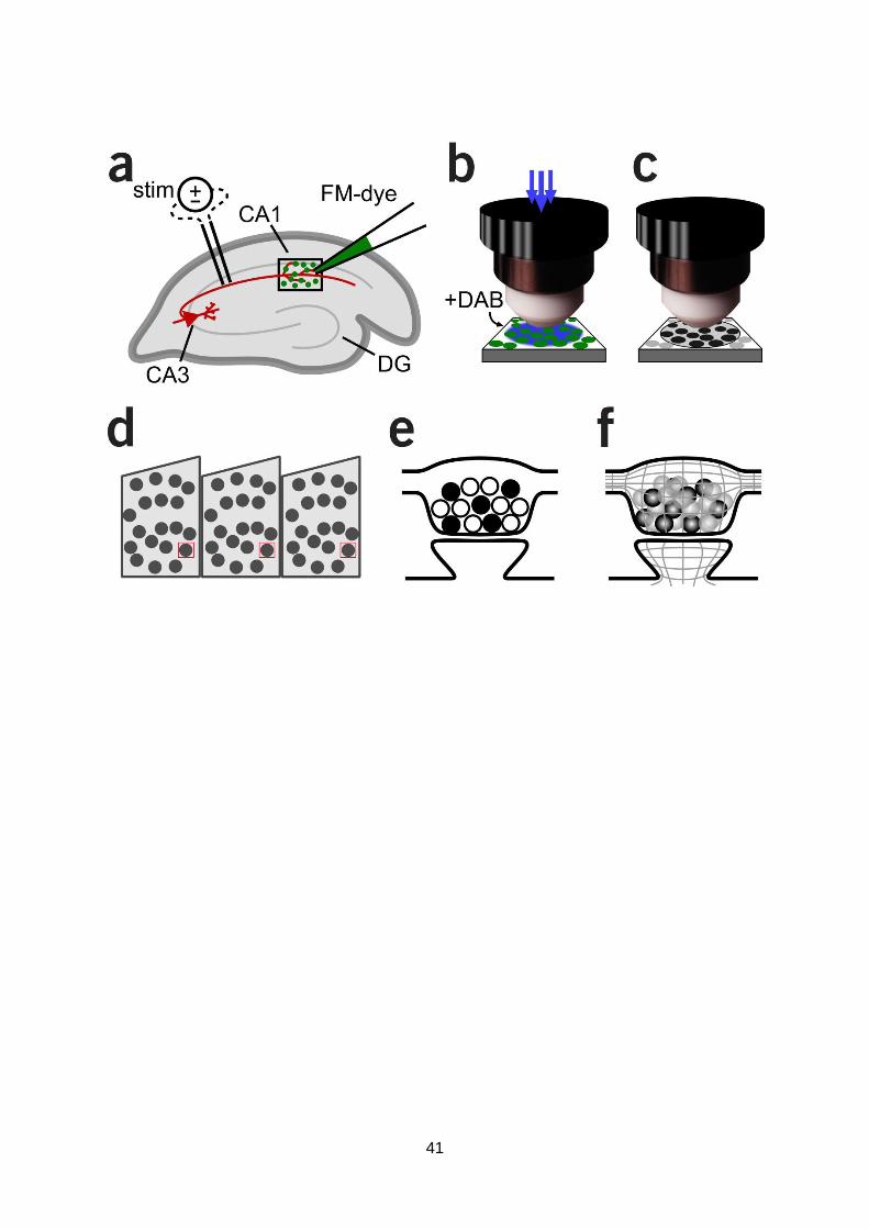
41

42

43
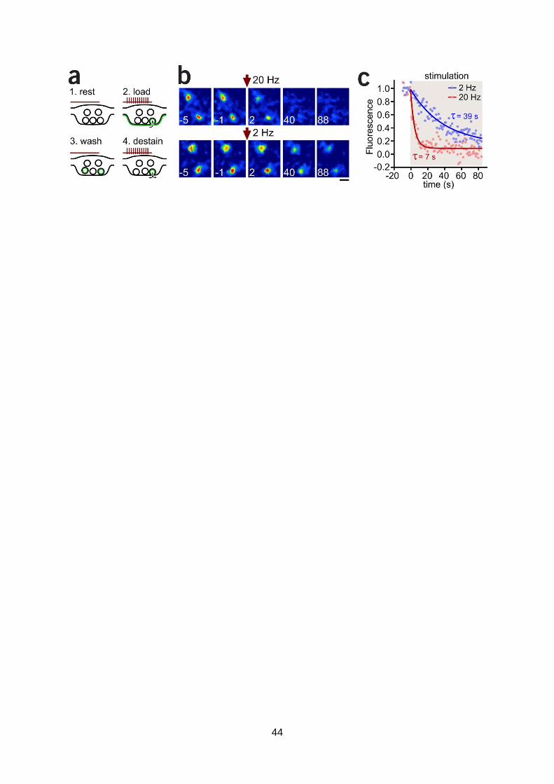
44
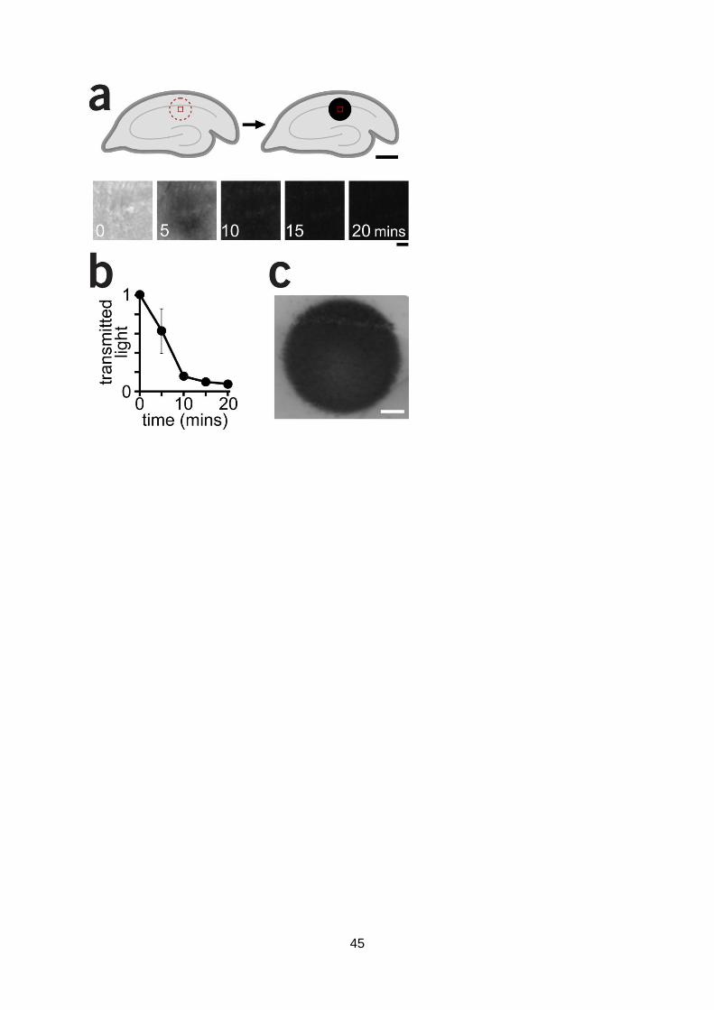
45

46

47