d o !>''' , , - national weather service · pmp estimates for 6, 24, and 72 hours...
TRANSCRIPT

HYDROMETEOROLOGICAL REPORT 'N0.53
L D ..... 'C..,p "\ ..u o tM/ 'A1 ws/t.d/M 'b
!>"'"'"' , , 1 1 ~, 5 E.~..~t:-west J/.,e; h~ s,J~ ..s, .... ~ ,41'b ~·qto
Seasonal Variation of 10-Square-Mile Probable
Maximum Precipitation Estimates, United States East of the 105th Meridian
U.S. DEPARTMENT OF COMMERCE ,_ , , --
NATIONAL OCEANIC AND ATMOS~HERIC ADMINISI'RATION
U.S. NUCLEAR REGULATORY COMMISSION - , -
Silver Spnng, Md , ,
Apn11980

U.S. Department of Commerce National Oceanic and Atmospheric
Administration
U.S. Nuclear Regulatory Commission
NUREG/CR-1486
Hydrometeorological Report No. 53
SEASONAL VARIATION OF 10-SQUARE-MILE PROBABLE MAXIMUM PRECIPITATION ESTIMATES) UNITED STATES EAST OF THE
105TH MERIDIAN
Prepared by Francis P. Ho and John T. Riedel
Hydrometeorological Branch Office of Hydrology
National Weather Service Washington, D.C.
April 1980

TABLE OF CONTENTS
Abstract. . . . . .
1. 1.1 1.2 1.3 1.4 1.5
2. 2.1 2.2 2.2.1 2.2.2 2.2.3 2.2.4 2.2.5 2.2.6 2.2.7
3. 3.1 3.2 3.3 3.3.1 3.3.2 3.3.3 3.3.4 3.3.5 3.3.6 3.4 3.4.1 3.4.2 3.4.3 3.4.4
3.5 3.6 3.6.1 3.6.2 3.6.3
4. 4.1 4.2 4.3 4.4 4.5
Introduction . Authorization. Purpose. . . . Scope ••... Definitions .. Previous study
Basic data . . . . . . . . . . . . . . . . . Background • • • • • . . Available station rainfall data ••
Storm rainfall • • • • • Maximum 1-day or 24-hour values, each month ••••••• Maximum 6-, 12- and 24-hr values, each month . 11aximum recorded rainfall at first-order stations. Data tapes, selected stations. Data tapes, 1948-73 •. Canadian data.
Approach to PMP. • ••. Summary. . . . . . . . . Selected major storm values •. Moisture maximization.
The concept. . . • • Atmospheric moisture Representative storm dew point • Maximum dew point. • . • • . Moisture adjustment. • • • . • Elevation and barrier considerations •
Transposition. . . •. • Definition .••..••• Transposition limits • • • • • • • Transposition adjustment . • • • • Distance-fro~-coast adjustment for tropical storm
rainfall. . . . . . . . . . . . . . . . . . . . . . . . Total storm adjustment . Envelopment. •
Durationally . Seasonally • Regionally •
Analysis • . • • Introduction . • • • . ~linimum PMP at 20 grid points .•.•••••••••••. Statistical computations of taped rainfall data (1948-73). Maximum observed rainfall values • • • • . Maximum atmospheric moisture •
iii
Page
1
1 1 1 1 2 2
2 2 3 3 3 3 3 3 5 5
5 5 5 6 6 6
15 15 15 15 16 16 16 17
17 17 20 20 20 20
20 20 21 21 28 28

4.5.1 4.5.2 4.5.3 4.6
4.7 4.7.1 4.7.2 4.7.3 4.8 4.9
5.
6.
7. 7.1 7.2 7.3 7.4
8.
Precipitable water in soundings .•.. Surface dew points . • . . . . • • . • • Seasonal variation of maximum moisture •
Seasonal variation of rainfall at selected long record stations (1912-61) . . . . . . • .
Rainfall depth-duration relations .• Within storms. Among storms . . . . . Analyses . • . . . . •
Regional PMP gradients Some observations on PMP
Resulting PMP.
Example of Use of PMP maps
Special problems . . . . .
patterns .•..•.
Stippled regions on PMP maps Extreme precipitation at Mt. Washington, ~-H • Point rainfall vs. 10-mi2 average rainfall. Storm adjustments greater than 150 percent .
Observed storms within 50 percent of PMP
Acknowledgements References
la
lb
lc
2
3
4
Sa
Sb
FIGURES
Storms controlling PMP (September through June) for 6 hours.
Storms controlling PMP (September through June) for 24
Storms controlling PMP (September through June) for 72
Grid points used for transposition . . . . . . . . . . Distance-from-coast adjustment for transposing tropical
storm rainfall (from HMR No. 51) . . . . . . . . . . 6-, 24-, and 72-hr PMP for grid point 11, (37°N, 89°W)
(Data are moisture maximized and transposed storm rainfall depths ...........•......
4% probability values for 6-hr duration for November
hours
hours
.
.
.
.
Ratios of 4% probability values for 6-hr duration for November or Decenber to the highest of the 12 monthly values. . . . .
iv
Page
28 29 29
29 29 29 38 38 46 46
48
48
48 48 80 80 81
81
86 87
11
12
13
18
19
22
24
25

Sc
Sd
6a
6b
6c
6d
7a
7b
7c
8
9
lOa
lOb
11
12
Seasonal variation of ratios of monthly maxima to the highest monthly 4% probability values for 6-hr duration (grid points 3, 6, 12, 13, 17, 20) •••••••
Month of maximum 4% probability values for 6 hours.
Example of analyzed maps of greatest observed 6-hr rainfall (November) • • • • • • • • • • • •
Example of analyzed maps of greatest observed 24-hr rainfall (November) . . • . • • • • • • ••
Example of analyzed maps of greatest observed 72-hr rainfall (November) • • • •
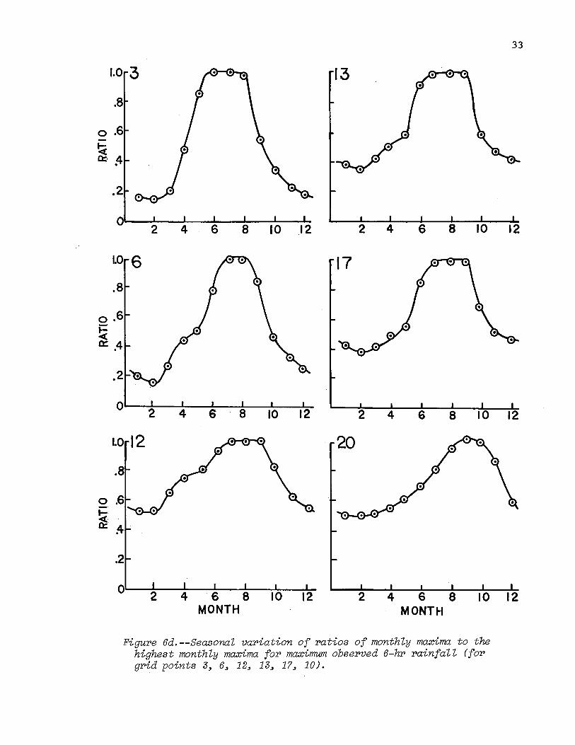
Seasonal variation of ratios of monthly maxima to the highest monthly maxima for maximum observed 6-hr rainfall (for grid points 3, 6, 12, 13, 17, 20) .
Contiguous United States, maximum w (mm), surface to 500-mb, by h~lf months, Januar~ through June (from Ho and Riede1,1979) •••.••.••••.
Maximum 12-hr persisting 1000-mb dew points (°C) for October (Environmental Data Service, .1968). • • . • .
Seasonal variation of ratios of atmospheric moisture for each month to that for the highest month (grid points 3, 6, 12, 13, 17, 20) ..••..••.••
Example of seasonal variations of 1% and 4% probability values, the maximum of record, and the ratio of each month's 4% probability value to that for the highest month. Three day rainfall for Duluth, Minnesota and Kansas City, Missouri (1912-61). Vertical scale gives both percentages, and depths in tenths of an inch • . • • • • . . • • • . • •
Seasonal variation of within storm 6/24-hr rain ratios for major storms in the study region • • ••
Within storm 6/24-hr rain ratios, January
Within storm 6/24-hr rain ratios, July ••
Within storm 6/24-hr rain ratios vs. magnitude of 24-hr depths. • . . • . • • • • • • •
Seasonal variation of within storm 72/24-hr rain ratios for major storms in the study region. • . . . . • . •
v
Page
26
27
30
31
32
33
34
35
36
37
39
40
41
42
43

13
14
15
16-25
26-35
36-45
46
47
Within storm 72/24-hr rain ratios vs. magnitude of 72-hr depths. . • . . . . . . • • .•...
Depth-duration plots for November (grid points 3, 6, 12, 13, 17, 20). Upper curves are the ratios of rainfall for various durations to the 24-hr value (+ from PMP; X from 4% probability values). Lower curves show PMP values. Maximized rainfall values transposed to the grid point are shown with storm number (table 2).
Latitudinal variation by month of 6-hr PMP along longitude 91°W . . . . . . . .
6-hr 10-mi2 PMP, January through December, (in.) . 24-hr lO-mi2 PMP, January through December , (in.).
72-hr lO-mi2 PMP, January through December , (in.) .
Example of variation of Pt~ depths with duration for midmonth of March and April for 40.5°N,87.5°W (see sec. 6).
Number of separate storms with rainfall ~ 50% of PMP for 6, 24, and 72 hours (number of storms ~·50% of P~W for July and August can be obtained from Riedel and Schreiner 19 80) • • • • • • • • • • • • • • • • • • • • • • • • • • •
TABLES
Pa.ge
44
45
47
49-58
59-68
69-78
79
82
l, Data sources for determining maximum station precipitation of record. . . . . . . . . • . • . • . . . . • . . • • 4
2 Major storms selected for moisture maximization and transposition. • . . • . . • . . • 7-10
3 Important storms centered in Canada near the U.S. border 14
4 Statistical analyses for 1948-73 station precipitation on magnetic tapes . . . . • . . • . . . . . • 23
5 Extreme precipitation amounts observed at Mt. Washington, N.H. (44 °l6N; 71 °l8W) during the winter season . 81
6 Known storm rainfalls for 6, 24, and 72 hours that are within 50 percent of mid-month PHP for the month in which the storm occurred (July and August storms not included) . 84-85
vi

SEASONAL VARIATION OF 10-SQUARE-MILE PROBABLE MAXIMUM PRECIPITATION ESTIMATES UNITED STATES EAST OF
THE 105th MERIDIAN
Francis P. Ho and John T. Riedel Hydrometeorological Branch
Water Management Information Division Office of Hydrology
National Weather Service, NOAA Silver Spring, Maryland
ABSTRACT. Estimates of the upper limit to rainfall that the atmosphere can produce (probable maximum precipitation) are given in this study for durations from 6 to 72 hours for each month of the year for 10 mi2 areas. The results are in a generalized form, that is, on maps allowing use for planning and design of any present or proposed hydrologic structure for the United States east of the 105th meridian. The probable maximum precipitation estimates show a smooth variation with duration, season, and location.
1. INTRODUCTION
1.1 Authorization
This study was authorized and funded through Interagency Agreement No. NRC-01-77-113 between the Nuclear Regulatory Commission (NRC) and the National Oceanic and Atmospheric Administration (NOAN dated June 2, 1977. The Agreement was extended to October 1, 1979, by an amendment dated May 20, 1979.
1.2 Purpose
The purpose of the study is to give seasonal variation of probable maximum precipitation (PMP) estimates for 10 mi2 areas for the United States east of the 105th meridian. PMP estimates for durations of 6 to 72 hours, by 6-hr increments are required.
1.3 Scope
PMP estimates for 6, 24, and 72 hours are given on generalized maps for each midmonth for 10 mi2 areas. While smaller sized areas have greater PMP values, especially for the warm season, they will not be defined in this study. For the winter season, PMP for smaller areas are not appreciably different from the 10-mi2 values in this study.
All-season estimates of PMP, Hydrometeorological Report (HMR) No. 51, FTobabZe Maximum Precipitation Estimates 3 United States East of the 105th Meridian3 (Schreiner and Riedel 1978) set the greatest values that can be

2
reached at some time during the year. They are accepted as upper bounds for the present study.
.1 .4 Definitions
ProbahZ.e maximum proecipitation (PMP) means th.e theoroeticaUy greatest depth of proecipitation foro a given dur.ation that is physicaZ.Z.y possibZ.e overo a paroticuZ.aro drainage basin at a cerotain time of yearo. (American Meteorological Society 1959). Realizing there are yet unknowns in the physical processes responsible for extreme rainfall, we refer to PMP values as estimates.
GeneroaZ.ized PMP estimates are estimates determined for large regions that are now required or one would expect will be needed in the future. These are frequently presented as a series of isolines on a map for a given area size and duration.
AU-season PHP is the greatest PMP regardless of season. For the region of this study one can generally say that for all durations, the all-season PMP will fall sometime between June and September for every point. Our problem is to determine the variation from this all-season estimate for each month of the year.
1.5 Previous Study
The only other study covering seasional variation of PMP for the entire region is HMR No. 33 (Riedel et al. 1956). Because the all-season values of HMR No. 51 differ from those of HMR No. 33, it follows that the estimates for each month in HMR No. 33 also need revision. All facets of PMP for the region were restudied and therefore the seasonal values differ from those in HMR No. 33.
2. BASIC DATA
2 .1 Background
As in all PMP studies, basic data are the extreme record storm rainfalls. Storom RainfaZ.Z. in the United States 3 Depth-Aroea-Duration Data (Corps of Engineers 1945- ) is a kept-up-to-date catalog of many of the most extreme areal rainfalls. The data are maximum areal depths for standard area. sizes and durations. Data for more than 600 storms have been published in this catalog. Additional data come from unofficial sources developed by the Hydrometeorological Branch (Shipe and Riedel 1976).
Most of the storms include data from surveys after the storm or resulting flood, sometimes called bucket suroveys3 in which additional rainfall measurements are found. Some of these values are measured in regular rain gages, privately owned or owned by local agencies or companies but not included in usual published records. Other values are measured in small test tube type gages, oil cans, or buckets. Such unofficial catches are accepted after checks against other observations and weather patterns, discussions with

observers, and more recently, against radar echoes and satellite pictures. It turns out that the most extreme point rainfalls of record are almost entirely from unofficial sources. This should be expected since there is practically no chance that the most extreme rainfall of a storm would occur over a preselected gage site. A shortcoming is that only very limited surveys and studies have been made for "out of season" (that is out of the season giving most intense rainfalls of the year) storms. Thus, we must augment our sample with extremes from regularly reporting precipitation stations and recognize that these values may not include the most extreme falls.
2.2 Available Station Rainfall Data
Table 1 lists several data sets that were surveyed for obtaining the greatest rainfalls for each month.
2.2.1 Storm Rainfall
3
This means Storm Rainfall in the United States~ Depth-Area-Duration Data (Corps of Engineers 1945~ ) and the augmented computer file of storm data (Shipe and Riedel 1976). The greatest value for 6, 12, 24, 48, and 72 hours for each month were used from these sources.
2.2.2 Maximum 1-Day or 24-Hr Values, Each Month
These values (Jennings 1952) are for regularly reporting stations for the period of record through 1949. Because nonrecording stations are more numerous than recording stations and have longer records, the maximum values generally are from nonrecording stations.
2.2~3 Maximum 6~~12- and 24-Hr Values, Each Month
For 28 of the 37 states involved in this study, there are published (U.S. Weather Bureau 1951-61) maximum observed depths at recording stations for these durations for the period beginning, in most cases, in the 1940's and ending in 1950. Exceptions are the few recorders going back many years at "first-order" Weather Bureau (now National Weather Service) stations.
2.2.4 Maximum Recorded Rainfall at First-Order Stations
A paper (Jennings 1963) published the greatest depths at first-order stations for durations from 5 minutes to 24 hours for about 200 stations in the study region. This is for the period of record through 1961.
2.2.5 Data Tapes, Selected Stations
For about 50 stations in our study region, daily rainfall records have been put on magnetic tapes for the period 1912-61. From these tapes we can extract 1-,2-, and 3-day maxima for each of the 12 months.

4
Table 1.--Data sources for determining maximum station precipitation of record
Item
United States Data
Storm Rainfall
Technical Paper No. 16
Technical Paper No. 15
Technical Paper No. 2
Data tapes
Data tapes
Canadian Data
Storm Rainfall
Station Maxima
Type of Data
Primarily maximum known areal depths
Period of record
For greatest known storms - kept up to to date.
Maximum 1-day Through 1949 or 24-hr values, each month for regular report-ing stations
Maximum 1-, 2-, 3-, 6; Through 1950 . 12-& 24-hr values for each month
Maximum record- Through 1961 ed rainfall 5 min to 24 hr for 296 1st order stations
Daily precipi- 1912-1961 tat ion
a. daily & 1948-73 b. hourly pre
cipitation ·for reguular reporting stations
Similar to U.S. storm rainfall
Daily Observation
1941-1970
Remarks
Mainly for warm season
Available for 28 of the 37 states in study region
Available for stations in study region
More than 6500 stations
See section 2.2.7

5
2.2.6 Data Tapes, 1948-73
These tapes include all observed hourly and daily rainfalls for the period measured both at recording and nonrecording stations, updating to 1973 the published data of pars. 2.2.2 to ·2.2.5 for the durations we are interested in.
2.2.7 Canadian Data
The Canadians have summarized maximum rainfall depths in much the same way we have in the United States. They maintain a catalog Storm Rainfall in Canada of greatest areal rainfall depths (Atmospheric Environment Service 1961- ). Another publication (Atmospheric Environment Canada 1973) givesthe greatest single observed value for one day at each observing station for the period 1941-70. Yet another source (Department of Transport) lists the greatest single observed value for a day in the period 1931-58. A list of station locations (Department of Transpor~Meteorological Branch 1970) was helpful in locating extremes near the northern bound of our study region.
3. APPROACH TO. PMP
3. 1 Summary
Central to this study, as al.ready mentioned, is HMR No. 51. For at least one midmonth the values of the present study reach the all-season P~W of HMR No. 51 for every geographical point. The basic approach used in HMR No. 51 is the approach adopted here. We will not repeat the various techniques, steps, and tests fully detailed in that report. More generally, a manual of PMP (World Meteorological Organization 1973) which summarizes PMP procedures that have been used in the United States is recommended for any reader who wishes to pursue the topic further.
Development of PMP for each month consisted of the following operations on selected major record storm rainfalls.
a. Moisture maximization
b. Transposition
c. Envelopment
Brief discussions of these items follow. At times we extract liberally from HMR No. 51.
3.2 Selected Major Storm Values
From the data sources listed we extracted those values that could significantly influence the level of PMP after they are moisture maximized (par. 3.3) and transposed (par. 3.4), for September through June and any portion of the study region. This was done by first plotting the most extreme depths for a given duration from Storm Rainfall in the United States on 12 maps, one for each month. We then extracted the greatest station values from the other data sources and added them to the plotted maps if they were of the same general level or greater than those already on the maps. Such maps were plotted for extreme values for durations of 6, 12, 24, 48 and 72 hours. On these

6
maps we also plotted the most extreme rainfall values for the region adjoi:..1-
ing the United States from the Canadian data sources.
Table 2 lists the storms selected chronologically by month. We show the storm location by latitude, longitude, town, and State. The storm number we used is given, as well as the Corps of Engineers' assignment number (if there is one) from Storm RainfaZZ in the United States (Corps of Engineers 1945- ) and the source of the data. The observed depth for the most critical duration is given. Other information in table 2 is explained in par. 3.5.
Figures la, together with respectively.
lb, and lc show the locations of these most important storms the observed rainfall depths for 6-, 24-, and 72-hr durations
The month of occurrence is also given.
Table 3 lists the more important storms selected from the Canadian data. These have a bearing on the magnitude of PMP near the U.S. border.
3.3 Moisture Maximization
3.3.1 The Concept
Moisture maximization is increasing storm rainfall depths for the storm location and season, for higher atmospheric moisture than was available in the actual storm.
Signficant precipitation results from lifting moist air. Processes causing this lifting, associated with horizontal convergence, have been described in numerous texts. Various attempts at developing a model that will reproduce extreme rainfalls are hampered by the lack of sufficient data within storms to adequately check the magnitudes of horizontal convergence, vertical motion, and other parameters. Since measurements of these parameters during severe storms are not readily obtainable, the solution has been to use extreme record storm rainfalls as an indirect measure of parameters, other than moisture, that are important to such events.
We thus adjust storm rainfalls of record to the equivalent that would have occurred with maximum moisture and make the following assumption: The sample of extreme storms is sufficiently large so that near optimum "mechanism" (or efficiency) has occurred. By "mechanism" is meant a combinecl measure of all the important parameters to rainfall production, except moisture. The assumption thus circumvents a quantitative evaluation of "mechanism" and results in increasing the observed storm rainfall, assumed to occur with near optimum "mechanism", by an adjustment for moisture.
This assumption is probably most realistic when considering ali-season PMP. Having to spread the storm sample throughout the 12 months weakens the assumption and we compensate by more liberal'envelopment (par. 3.6).
3.3.2 Atmospheric Moisture
The best measure of atmospheric moisture through depth can be obtained from radiosonde observations. Specifically for the present study we have

Table 2.--Major storms selected for moisture maximization and transposition
Total CoE1 Gridpoint(s) Critical Obs. Controlling storm
Storm Location Assignment transposed Duration(s) Depth for grid adjustment Date Number Citl State Lat. Long. Number Source* to 'iJ (hrs) (in.) Eoint(s) ~)
1/18-21,1935 2 Hernando MS 34°50 90°00 LMVl-19 STR 6,7,10,11,13 72 13.4 6 70 1/1-2,1941 3 Pigeon River MI 48°00 89°42 T.P.l6 9,10 24 4.7 9,10 150 1/4,1949 4 Coleraine MN 93°28 47°16 DTD 1,5,9 1/22-27,1949 5 Timbo AR 35°52 92°19 SW3-10 STR 6,7,8,10 6 7.5 6,13 70
11,12,13 24 11.7 10 74 1/31-2/2,1920 6 St.Augustine FL 29°51 81°21 STR 12,15
2/14-19,1938 8 Calvin OK 34°56 96°15 SW2-17 STR 6,7,10,11 6 4.8 6 78 2/6,1955 9 Oberlin LA 30°36 92°47 DTD 12,15,17 2/22,1961 10 Bessemer AL 33°22 87°01 DTD 12,15,17 72 13.5 17 150 2/10,1966 11 Leesville LA 31°09 93°16 T.P.l6 7,8,11,12,15 2/26,1969 12 Mt.Washington NH 44°16 71°18 DTD a 72 14.1
2/10-11,1970 13 Mt.Washington NH 44°16 71°18 DTH a 24 10.2 2/1,1973 14 Spearsville LA 32°56 92°36 DTH 7 ,8,11,12 6 10.6 8,12 141
7,11 116 2/23-25,1875 15 Clingman Dome NC 35°33 83°30 STR 14,16 6 5.8 16 90 3/26-4/1,1886 16 Pinkbeds NC 35°22 82°47 STR 14 3/23-27,1913 17 Bellefontaine OH 40°22 83°46 ORl-15 STR 6,7,10,11,13 24 7.3 13 116
72 10.4
3/24-28,1914 18 Merryville LA 30°46 93°32 LMV3-19 STR 8,12,15 3/11-16,1929 19 Elba AL 31°25 86°04 LHV2-20 STR 8,12,15 6 14.0 8,12,15 134
24 20.0 72 29.6
3/28-4/2,1945 20 Van (nr) TX 32°20 95°42 SW3-5· STR 8,12 3/25,1964 21 Spruce Mt. NC 35°37 83°12 DTH 14 3/16-17,1965 22 Bayfield WI 46°53 90°49 DTD 9,10,13
1 110 3/2-5,1966 23 Courtenay ND 47°14 98°35 STR 1,5,9 24 4.7 5 116 3/14,1973 24 Lead SD 44°21 103°46 DTD 1,2,5,6,9,10 24 5.7 1,5,9 105
2 135 4/22-24,1932 25 Ellendale ND 46°29 99°45 STR 1,5,6,9,10 6 3.0 5,9 149
1 135
See last page for notes.
--.!

Table 2.--Major storms selected for moisture maximization and transposition (continued) 00
Total GaEl Gridpoint(s) Critical Obs. Controlling storm
Storm Location Assignment transposed Duration(s) Depth for grid adjustment Date Number City State Lat. Long. Number Source* to 'V (hrs) (in.) Eoint(s) (%)
4/11-14,1933 26 Durham NH 43°08 70°56 NAl-23 STR 17,18,20 6 4.9 18 150 20 142
4/3-4,1934 27 Cheyenne OK 35°37 99°40 SW2-ll STR 7,8 6 17.3 7 148 24 21.3 8 150
4/24-28, 1937 28 Clear Spring MD 39°40 77°54 SA5-13 STR 16,17,18 4/26, 1954 29 Morris MN 45°35 95°55 T.P.l6 5,6,9,10,13 24 6.9 9 148 4/23-24,1960 30 Gurney WI 46°28 90°30 P.P.l6 5,6,9,10,13
4/28, 1970 31 Hazelton ND 46°29 100°17 DTH 1,2,5,6,9,10 6 3.8 9 110 4/20-22, 1973 32 Moberly HO 39°28 92°25 DTH 9,10,11,13 24 8.3 13 122 4/12-14, 1974 33 Magee MS 31°55 89°42 STR 8,12,15 5/30-31, 1935 34 Hale co 39°36 102°08 MR3-28a/ STR 3 6 16.5 3 128
24 22.2 5/6-12,1943 35 Warner OK 35°29 95°18 SW2-20 STR 7,10,11 6 9.9 10 116
24 17.2 11 134 72 24.9 10,11
5/30, 1949 36 Thief Rvr Fll.s MN 48°07 96°11 DTD 1,5,9 5/28, 1961 37 Bar Harbor ME 44°23 68°12 DTD 18,20 6/13-18, 1886 38** Alexandria LA 31°19 92°33 LMV4-27 STR 8,12 6/17-21, 1921 39 Springbrook MT 47°18 105°35 MR4-21 STR 1,2 6/14-15, 1942 40 Warren lSE NH 43°55 71°53 T.P.l5 16,17,18,20
6/10-13, 1944 41 Stanton NE 41°52 97°03 MR6-15 STR 5,6,7,9,10 6 13.4 5,9 128 11,13 6,10 141
11 148 13 122
6/23-24, 1948 42 Del Rio TX 29°22 100°37 STR 4,8 24 26.2 4 121 6/23-28, 1954 43** Vic Pierce TX 30°12 101°35 SW3-22 STR 4,8 6 16.0 4 116
24 26.7 8 150 72 34.6 4,8
6/30, 1962 44 Cedar Is NC 34°57 76°17 DTD 17 6/23-24, 1963 45 David City NE 41°14 97°05 STR 5,6,7,9,10,11 6 14.6 5 128
6,9 134 10,11 141
See last page for notes.

Table 2.--Major storms seleeted for moisture maximization and transposition (continued)
CoE1 Total
Location Gridpoint(s) Critical Obs. Controlling storm Storm Assignment transposed Duration(s) Depth for grid adjustment
Date Number City State Lat. Long. Number Source to 'i/ (hrs (in.) point (s) _____{!)
6/24, 1966 46 Mellen Dam ND 47°21 101°19 STR 1,2,5,6,9 6 11.1 1 148 6/9,1972 47 Rapid City SD 44°12 103°31 MRl0-12 STR 2 6/20-22, 1972 48 Bolivar NY 42°05 78°10 STlt 16,17,18,20 24 14.3 20 121
72 18.5 9/8-10, 1921 49** Thrall TX 30°35 97°18 Gt14-12 STR 4,8,12,15 24 36.5 8,12 ll4 9/17-19,1926 50 Boyden IA 43°12 96°00 MR4-24 STR 5,6,7,9,10,ll 6 15.1 5,9 122
13 24 21.7 6,10 134 7 ,ll 141 13 128
6/16-17,1932 51 Westerly RI 41°22 71°50 NA1-20 STR 16,17,18,20 9/1, 1940 52** Ewan NJ 39°42 75°12 NA2-4 STR 17,18 6 20.1 17 128
18 122 9/2-6,1940 53 Hallet OK 36°15 96°36 SW2-18 STR 7,8,11,12 6 18.4 7,8,11,12 141
24 23 .. 6 9/3-7,1950 54** Yankeetown FL 29°03 82°42 SAS-8 STR 8,12,15,17 24 38.7 8 100
12,15 98 10/27-30,1900 55 Bedford IA 40°53 94°34 UMV1-7A 6,9,10 6 5.0 9 122
10/7-ll,1903 56 Petersburg NJ 40°55 74°10 GL4-9 STR 16,17,18 10/17-22,1941 57** Trenton FL 29°48 82°57 SA5-6 STR 8,12,15,17 24 30.0 8,12,15 ll6
72 35.0 17 llO 10/11-18,1942 58 Big Meadows VA 38°31 78°26 SA1-28A STR 16,17,18 24 13.4 18 150
72 18.7 10/9-10,1954 59 Aurora IL 41°45 88°20 STR 10,13 24 11.7 10 150 10/25,1959 60 Pinkham Notch NH 44°16 71°15 DTD 16,18,20
10/3-4,1969 61 Hartford CT 41°50 72°54 STR 15,16,17,18 10/4, 1971 62 Mt. Weather VA 39°04 77°53 DTH 16,17,18 10/10-11,1973 63 Enid OK 36°25 97°52 STR 6,7,10,ll 6 16.9 ll ll6
24 18.6 6,10 100 7 llO
ll/1, 1909 64 Ironwood MI 46°27 90°ll T.P.l6 5,6,9,10 ll/7, 1915 65 Crosby ND 48°54 103°18 T.P.l6 1,2,5,6 11/12-15,1922 66 Lakeside LA 30°02 92°30 LMV3-29 STR 8,12,15
See last page for notes.
""

Table 2.--Major storms selected for moisture maximization and transposition (continued)
Location
Date Number City State Lat. Long.
11/2-4,1927 67 Kinsman Notch NH 44°03 71°45
11/15-17,1928 68 lola KS 37°55 95°26
11/22-25,1940 69 Hempstead TX 30°08 96°08
11/1, 1969 70 Fernandina Ech FL 30°41 81°28 12/5-8, 1935 72 Satsuma TX 29"54 95°37
12/29-1/1/49 73 Berlin NY 42°40 73°19
12/27, 1969 12/10, 1971
74 75
Mt.Washington NH 44°16 Vallient OK 34°00
NOTES:
1. CoE: Corps of Engineers
* Source (refer to table 1)
STR: Storm Rainfall
T.P. 16: Technical Paper No. 16
DTH: Data tape; hourly precipitation
DTD: Data tape, daily precipitation
**: Distance-from coast adjustment used.
V See figure 1 for grid point locations
a: not transposed (see par. 7.2)
71°18 95°06
CoE1 Gridpoint(s) Critical Obs. Controlling Assignment transposed Duration(s) Depth for grid
Number Source'' to V (hrs) (in.) Eoint(s)
NAl-17 STR 16,17,18 6 7.8 16,18 24 12.0 72 14.0
MR3-20 STR 6,7,10,11,15 24 9.0 6 10
Gl1.5-13 STR 7,8,11,12 24 18.6 7 72 21.1
DTD 15,17 GM5-4 STR 8,12,15 24 18.6 8,12,15
72 20.8
STR 18 6 3.5 18 24 8.1 72 12.6
DTD a DTD 7,11
Total storm
adjustment (%)
141
111 122 100
150
150
I-' 0

LEGEND 17.3-PRECIPCIN)
• 4-MONTH 251 2
C 7)-STORM INDEX NO.r1
CSEE TABLE 2) 119. 115• 111. 107.
103. 99° 95° 91.
103. 99. 95. 91.
FigUPe la.--Storms controZZing PMP (September through Jun~for 6 hoUPs.
STATUTE MILES
190 ? 1\)0 , 390 100 0 IOo :260 300 :(&)
KILOMETERS
87. 79. 75.
t--' t--'

LBGEND 261-PRECIP CIN)
usJ •6 -MONTH 251 \C43)-STORM INDEX NO.
\ CSEE TABLE 2) DURATION IF NOT 24HRS1
119' 115° 107' 103°
103° 99° 95' 91°
99' 95' 91'
Figure lb.--Storms controlling PMP (September through June) for 24 hours.
87' 83'
STATUTE MILES
190 ? 12io 2,90 390 100 0 160 0 300 ~110
KILOMETERS
79' 75'
1-' N

LEGEND 34.6-pRECIP CIN)
[4sJ. 6 -MONTH 25"1 /c43)-STORM INDEX NO. ~ (SEE TABLE 2) DURATION IF NOT 72HRS
119° 115° 111°
103° 99°
!_ I , ___ , ___ . __
107° 103° 99°
95° 91°
\ -j \
95° 91° 87.
Figure lc.--Storms controlling PMP (September through June) for 72 hours.
STATUTE MILES
100 0 190 2(/0 390
1 bo 6 ulo 26o 300 400 KILOMETERS
79° 75°
1--' w

14
Tab Ze 3. --Important storms centeroed ~-~n Canada near the U.S. border
Rain-Location Critical fall
Storm duration(s) depth Date no. City Province Lat. Long. (hr) (in.)
1/15-17,1958 76 Liverpool NS 44°08 64°56 24 5.8 60 10.0
3/31-4/2,1962 77 Alma NB 45°36 64°57 24 9.3 5/25-28;1961 78 45°47 66°45 6 4.0
24 9.5 72 11.8
5/30,1961 79 Buffalo Gap Sask. 49°07105°17 6 10.5 6/29-7/1' 1935 80 Tilson Man. 49°22 101°18 60 13.0 9/20-23,1942 81 Stellarton NS 45°34 62°39 72 13.4
therefore published (Ho and Riedel 1979) the maximum observed semimonthly precipitable water (w or depth of liquid equivalent of the water in a column of air) for mo~e than 100 stations for the period of record. This information was useful guidance. However, radiosonde data alone cannot be used for moisture maximization for several reasons. First, many extreme storms occurred before the radiosonde network was established. Second, the radiosonde network is too sparse to detect narrow tongues of moisture that are important to many storms. The solution was·to use surface dew points, which are observed by many stations, as indices to atmospheric moisture. A saturated pseudo-adiabatic atmosphere is assumed, tied to surface dew points, which fixes the moisture and its distribution with height in the atmosphere. Tests have shown that the moisture thus computed is generally an adequate approximation to atmospheric moisture in major storms or for high dew point situations (Miller 1963). For a saturated pseudo-adiabatic atmosphere, tables have been prepared (U.S. Weather Bureau 1951) giving wp values based on 1000-mb dew points.
Two dew points are required for moisture maximization. One is the dew point representative of moisture inflow during the storm. The other is the maximum dew point for the same location and time of year as the storm. Both storm and maximum dew points are reduced pseudo-adiabatically to 1000 mb to normalize for differences in station elevations.
Both storm and maximum dew points are usually taken as the highest value persisting for 12 hours. Instantaneous extreme dew point measurements may not be representative of inflow moisture over a significant time period. Also, taken over a duration, the effect of possible erroneous instantaneous dew point values is reduced.

15
3.3.3 Representative Storm Dew Point
Dew points are selected in the warm moist airflow into the storm. Both distance and direction of the dew points from the rainfall center are recorded. An average dew point value from several stations is considered to give the best estimate. Care must be used to insure that dew point observations are taken within the moist tongue involved in the heavy precipitation. The time sequence of dew points from each station is reduced to 1000mb before averaging. After averaging, the highest persisting 12-hr value is selected.
3.3.4 Maximum Dew Point
Maximum dew points are generally the highest dew points observed for a given location and time of year. These dew points are based on seasonal and regional envelopes of maximum observed surface dew points that have persisted for 12 hours, reduced to 1000 mb,at many stations (Environmental Data Service 1968).
We adjust the storm to the maximum dew point 15 days from the storm date into the warmer season except for one case, the Hale, Colo., storm of 1935 which was accompanied by unusually cold air judged to be dynamically significant to the rainfall. Moisture maximization adjustments are increased by up to 10 percent by the 15-day seasonal transposition into the warm season. In the cool season (December-February), the 15-day leeway usually does not change the moisture adjustment.
3.3.5 Moisture Adjustment
Moisture maximization is accomplished by multiplying observed rainfall by the moisture adjustment, which is the ratio of w for the maximum 1000-mb 12-hr persisting dew point to the w for the sto¥m 1000-mb 12-hr persisting dew point. Theoretical justificatign for this adjustment is found in HMR No. 23 (U.S.W.B. 1947). This maximization expressed mathematically is:
where
p
w p
3.3.6
w p X p (maximum)
w (storm) p
moisture adjusted rainfall
observed rainfall
precipitable water. (Maximum) refers to enveloping highest observed w and (storm) refers to the storm w. (Both dew points are for the sa~ location.) p
Elevation and Barrier Considerations
Where there is a significant mountain barrier between the moisture source and rain location, or the rain occurs at high elevations, a refinement is sometimes applied to the moisture adjustment. In such cases, mean elevation of the barrier ridge, or elevation of the rainfall rather than the lOOQ-mb surface, is used as the base of the column of moisture. For the region of

16
our study, location of representative storm dew points -(usually toward a coast and at lower elevations) and restrictions to storm transposition (par. 3.4.2) generally eliminated the need for using elevation in the moisture adjustment.
3.4 Transposition
3.4.1 Definition
Transposition means relocating storm precipitation within a region that is homogeneous relative to pertinent terrain and meteorological features.
3.4.2 Transposition Limits
Topography is one of the more important controls on limits to how far storms can be transposed. If observed rainfall patterns show correspondence with underlying terrain features, or indicate triggering of rainfall by slopes, transposition should be limited to areas of similar terrain. Identification of broadscale meteorological features is important, e.g., surface and upper air high- and low-pressure centers that are associated with the storm, and how they interact to produce the rainfall. Thus, useful guidance to determining transposition limits are storm isohyetal charts, weather maps, storm tracks, rainfalls of record for the type of storm under consideration, and topographic charts.
The more important limits to storm transposition for this study were:
a. Transposition was not permitted across the generalized Appalachian Mountain ridge.
b. Tropical storm rainfalls were not transposed farther away from nor closer to the coast without an additional adjustment (par. 3.4.4) in cases where the maximum dew point charts showed no variation.
c. In regions of large elevation differences, transpositions were restricted to a narrow elevation band (usually within 1000 feet of the elevation of the storm center).
d. Eastward limits of transposition of storms located in the Central United States were the first major western upslopes of the Appalachians.
e. Westward transposition limits of storms located in Central United States were related to elevation. This varied from storm to storm but in most cases the 3000- or 4000-ft contour was used to set the limit.
f. Southward limits to transposition were generally not defined since other storms located farther south usually provided higher rainfall values.
g. Northward limits were not defined if they extended beyond the Canadian border (the limit of the study region).
We used a simplification in transposing by making decisions for each critical storm on whether or not to transpose to each of 20 grid points

covering the study region. These points are shown on f.igure 2. A similar set of points was used as a test in the all-season study (HMR No, 51} ~or transposition rather than setting outer bounds. After regional smoothing, thus extending the influence of major storms, the results of the two techniques are similar for the area size of this study.
3.4.3 Transposition Adjustment
The transposition adjustment applied to relocated rainfall values is the ratio of w for the maximum 12-hr persisting dew point for the transposed location tg that of the storm in place. The maximum dew point is for the same distance and direction from the transposed location as the storm representative dew point is from the storm location (par. 3.3.3).
3.4.4 Distance-From-Coast Adjustment for Tropical Storm Rainfall
17
The general decrease in tropical storm rainfall with distance inland is well known. It is attributed to the difficulty of maintaining the same rainfall intensity as distance from the moisture source increases, and to the deterioration of the tropical storm circulation with increasing distance inland.
A study (Schwarz 1965) developed a relation showing the distance in tropical rainfall with distance up to 300 n.mi. inland. The relation was basedon both observed and moisture-maximized tropical rainfall data for several area sizes and durations. Figure 3 shows this variation along with its extension for distance farther inland. It shows no decrease in rainfall for the first 50 n.mi. inland from the gulf coast, a smooth decrease to 80 percent at 205 n.mi. inland, and 55 percent at 400 n.mi. inland.
We applied the adjustment for distance-from-coast to tropical-storm rainfall (all durations) transposed within the region where the maximum 12-hr persisting dew point charts (Environmental Data Service 1968) indicate no variation. When transposing tropical storm rainfalls farther from the coast, the values are decreased. In the same way, they are increased when transposed nearer to the coast.
Of the major rains shown adjustment to six storms. by the storm number.
3.5
in table 2 we applied the distance-from-coast These storms are identified with a double asterisk
Total Storm Adjustment
Table 2 includes the grid points to which the selected major storm rainfalls were transposed, the grid point where the storm was most important, and the total adjustment to the rainfall for those grid points. This total adjustment is the product of the adjustments for maximum moisture and for storm transposition; the latter was determined either from maximum dew points or from the distance-from-coast relation.

103° 99'
l,""-,1
\_4 ,.J,(-"'',,
\ '-:
107' 103' 99'
Figure 2.--Grid points used for transposition.
95'
i --1_1
95'
I l \
91'
j
91' 87'
ST .e. TUTE MILES
IQO 0 190 2QO 3QO
100 6 100 260 300 400
KILOMETERS
79' 75'
1-' CXl

lOOtt-----
1-Cl)
< 90 0 u 1-< w ::> 80 _, < >
~ 701 z w u a=: w I:L.
6d
50
~ADOPTED ADJUSTMENT SCHWARZ ( 1965) WITH EXTENSION
100 200 300 400 DISTANCE FROM COAST
Figure 3.--Distance-from-coast adjustment for transposing tropicaZ storm rainfaZZ (from HMR No. 51.).
N.MI.
1-' \.0

20
3.6 Envelopment
Moisture maximization and transposition of major storms to the 20 grid points set the very lowest value of PMP for each month at these points. How much to envelop these values and give consistent PMP from place-to-place, month-to-month and duration-to-duration is the major portion of this study.
3.6.1 Durationally
By this we mean smooth curves of rainfall depths extending from one duration to another. Such smooth curves imply that the storm record has given more extreme depths for certain selected durations than for others.
3.6.2 Seasonally
Seasonal envelopment, in much the same context as in durational envelopment, assumes the storm record does not provide equally extreme depths for all months. We thus draw smooth seasonal curves for a selected grid point, enveloping all of the data for some months.
3.6.3 Regionally
We assume that except for topographic and coastal influences we should have a smooth regional pattern of PMP.
4. ANAfuYSES
4.1 Introduction
We have set the stage by describing the available data and the basic concepts that bear on the results and on how these results will be reached. We now give details of the data analyses leading to our goal.
One additional consideration entering into our procedures is how to show results concisely but fully, that is, how to show PMP for durations for 6 to 72 hours for 10 mi2 for each month for the study region. Tests have shown that for a point east of the 105th meridian when PMP values for 6, 24, and 72 hours are plotted on linear graph paper(duration vs. depth) and joined by a smooth curve through the point of origin (0,0) the curve adequatelydefines PMP by 6-hr increments to 72 hours. We decided to present maps covering the region for each month showing PMP depths at midmonth in inches, for 6, 24, and 72 hours. (For July and August, the mapped values turn out to be identical to the all-season PMP of HMR No. 51 and to each other for the entire study region. Similarly, the PMP values for January and February are the same).
In our approach, we need to take care that the smoothing procedures give PMP values that are not unrealistically extreme: each smoothing step, if not done with care, could give a cumulative envelopment that results in an unreasonably large final product. This concern must be balanced with the basic need -- that at the least, all known observed rainfall depths maximized for moisture should be enveloped. Further, our results should, to the best of our capability, give extremes that will not be exceeded by future storms.

21
4.2 Minimum PMP at 20 Grid Points
Seasonal plots were made for each of the 20 grid points (fig. 2) of the greatest moisture maximized and transposed from depths for 6, 12, 24, 48, and 72 hours. We then drew tentative smooth enveloping curves for these data for 6, 24 and 72 hours on each plot. An example of these plots and in this case the final smooth enveloping curve is shown in figure 4. The storms on the figure (identified by a number near the X axis) can be identified by storm number in table 2.
The remainder of chapter 4 gives analysis of various rainfall data that was helpful in decisions on how to obtain a consistent set of PMP values for all durations, months, and locations.
4.3 Statistical Computations of Taped Rainfall Data (1948-73)
Using computer programs we determined a variety of products that could influence or give guidance to our study. The first simple product, of course, is a tabulation of the greatest observed depths for a specified duration for each month of observation. Such maxima lend themselves to statistical analysis.
From the rainfall for each station recorded on tape with 20 or more years of record, the maximum values for each month for a duration of interest were put into series of all January maxima, all February maxima, etc. To each series we fitted the Fisher-Tippett type I distribution by the Gumbel fitting procedure. This statistical distribution is used almost exclusively by the National Weather Service, for precipitation frequency analysis (Hershfield 1961 and Frederick et al. 1977).
From the fits, the rainfall amounts with 0.04 and 0.01 chance of being equalled or exceeded for each month at each station were abstracted (hereafter referred to as 4 percent and 1 percent probability level rainfalls). These rainfall amounts for all stations located with each 2° latitude and longitude quadrangle were then averaged. This was done for quadrangles overlapping (both in the north-south and east-west direction) by 1° latitude and longitude, respectively. This averaging was a smoothing step.
Table 4 summarizes the statistical analyses for 6, 24, and 72 hours. The sets of 4 percent and 1 percent probability level and maximum values which were computed and plotted on maps using a computer program are indicated in table 4, part 1. Figure Sa is an example of the 6-hr 4 percent probability level values for November and their analyses.
Part 2 of table 4 refers to maps of the ratios of monthly values to the maximum value for any one of the 12 months. These ratios are guides to the corresponding ratio of monthly PMP to all-season PMP. Figure 5b is an analyzed example of these ratio maps for the 4 percent probability level amounts for 6 hours for November. The values shown in this figure came from combining the ratios in each quadrangle for the months of November and December. The highest ratio of the two months was selected and plotted.

-LEGEND
72HR X-72 HR
16-48 HR •-24 HR
24 HR " j0-12 HR +-6 HR
&
6HR
~ 24f _// / ~e
+ 0
+ + + + 0
A + • • G)9 • •
+ • 0 + ~ +
0 + + 2,5,14,11,8
I I I I I I I I I I I I
JAN FEB MAR APR MAY JUN JUL AUG SEP OCT NOV DEC JAN MONTH
Figu:re 4.--6-_, 24-_, and ?2-hr PMP for grid point 11_, (3? 0 N_, 89°W) Data are moistu:re maximized arid transposed storm rainfaZZ depths.
N N -

Table 4.--Statistical analyses for 1948-73 station precipitation on magnetic tapes
*4% *1% maximum
Part 1
12 maps,each 6 hr X X X duration, in 12 hr X X X inches 24 hr X X X
1 day X X X 2 day X X X 3 day X X X
Part 2
12 maps, each 6 hr X X X duration,% 12 hr X X X of highest 24 hr X X X month 1 day X X X
2 day X X X 3 day X X X
Part 3
2 maps,each 6 hr X X X duration of 12 hr X X X month of 24 hr X X X maximum and 1 day X X X and·mini- 2 day X X X mum 3 day X X X
Part 4
12 maps,each 6/24 X X X rain ratio 12/24 X X X
72/24 X X X
*4% and 1% probability values based on Fisher-Tippett Type I distribution fitted by the Gumbel procedure.
23

N "" "" "'" "'" (II (II 0 (II 0 (II 0 z z z z z z
I J·' :;2 ~·~
.,, 70 70 ., <.o ~' 'ti.' .. •.. 4:; I ··~ '·~ ;.· I ~ 2 5 • " ,; I, I 7 ' " 1' 1• ' I
I 11.") I ···I I te:) ;O "'' [!.1 ~L_!.IL "f- _J:h--fl (.4 '+.j ·,~ I•• ,,, ., /·"•
~ 1 ' , :J 5 'J ~ b J·' I ·' I ~ ··. ,, I I
I (\) 15 I"' 3J "' .,, " 3 , .; " ' 7
tr, I 1--~
,, •• I"~ ., ;o 117 '1;- I 1 • ,; , I
I 0 .. 1, f:».; :l:j I I 0
~ 0
I I 0 ~ ~ ~ 10 I'~ '?-; '" .-,.,.
"' I 9 ., ' • ; '\j I
I ~ '" <If.',
~ .. ~ ~ "' G• •o _,,,._1 ~ ~ u,.... .... y-""""'J- ")
"· '" I N ;.~
"· 1
<:i- .. - I ~ co
(II
~ ~
N ~ (\) rn
~ "'S 0';) co I co ;::s-> 0 0
"'S ~ ~
~ ~ <:i-
"· () ;:s
~ ~I ~~~5dP4 2~3 21•t 2231 2~ I 183 f lf,~ '"
]0::!/ llft 1~a~~ I I~ "'S E
b 5 15 1 C""'Q.5-
I ) ~ tb
(...J
...... 11
~ ~ (\)
§. (\) "'S . ~~:z
)( X X X X
z-+> oZ"::J!. • 0
oi-u C:::o -nzor
lflCitllrn j;!fR6;G.> :...to-rn
~I 10 -=-~c zl I ~~ "fL~~Z' ]:H) l'ln )tD I~ zi-to 7 rs ~7( 2f- 2u\ 1~ l/)0-< /
-n,.::::: l>l> ZE zrn 0 I
= N "" "" "'" '"(; "'" (II
(II 0 (II 0 (II 0 z z z z z z
i]Z

1\) "' "' .:> .:> U1 U1 0 U1 0 U1 0 z z z z z z
~ '3':i ;Jo.~ 2;.•J ~, ~ . J'l c ~ 2 5 9 ]5 1~
~~~.w 2.\5 213 tnt, l~o inl tY3 1•1:-. 17'"1 ,q,_. ~ ~ ~ 1 9 JJ J ll. (,
1 r. q (.
;:s-' I ' I {\) t:rl 3 11':1 .:S 1tt 2.''!1 q...-.-....9,'}::» til9 i:=-."i tr.g , r·, I
~::)" 0 " G 7 ' 3 I ' .) 7 L_-f....l'"
1 243 2~5 h::' 111 1'11 I
~. 7 • I' ,, I I I
~ ~ i5 ,, I i5 Cl~ 0 ., I o ~ ~ ::E I ::e ~.~. ,1, 1
;:s-'Cl " ~~ I ~ - 53'l &oo 551 3'17 . 48 pl4n 112. I
Cl g~ ~~
~ ~ ~'\::l
"':: co Cl U1 ~::)" ::e
§. ~. ~ ~.
~ g ~
~ co co ~ 0 0 ~ ::e ::e
~ "'::
~ I
~ P...
~ <»I \f\{~j 096 '"' E~~·' w t '~~11 6~ ••P• ~•·• ''"
3 ''I"~~ 1 I<» "':: U1 I 1 1& 22 2vrsl 19 1 c . -r- 11 r. s s U1 ~ ::E ' J . I ::E ~ ~. Cl ~
~ "'::
~ ~ <»-~ X ~ 0 X X 3! ::E X X
0' d z:::o ~ \; p~ Cl ~ oo "':: .£:::;::! , - r
lflz ITI
~ -1-1 ~ Q ~Iz ~ -Oo :0! oc ~ ~ Zlfl I I r~~d., ... t" ~ I~ ~ (II IJ'Il> 7 " ' 2& 20 , 3 • (II
"':; ::E Z I ::E o m
~ -1 Cl I
(j'l
£t. ~
;:s-'
~ ~ ~ ------ --- ~ ~ ~ ~ g; ~ z z z z z z (J.)
~
S'Z

26
0 -~ 0::
20
Figure 5c.--Seasonal variation of ratios of monthly maxima to the highest monthly 4% probability values for 6-hr duration (grid points 33 63 123 133 173 20).

SON IOOW 95 W 90 W 85W BOW 75W SON I
_____ j__
JUNE
-- -(----~ '~ ..... ~...- '\r--......_r---
\ I \ \
--,.-j ·r"' -- \
45NI I ) I L 1 ~\( /':(,- f .· -~ \ "t""" ~ j 'l ,, ' """I . ~,,
-------
~ ... ~ ":·· -----J"\41LY
---.. -·- '/"'-_.....,. ,..;.._;. _ _l_ -l ,,
I ,_ J' ,.~
I 'J
40NI I I -'f=--=--=-\, 1 ' ';- ' t ' ' - /1~:.: ~ I"' ·'--) . ) -I
T f
__ I"j_ __ _
r-----7 -l
I 35 NI I I ·/' " j. I ~ 0 ~ y A - t - - I t ""' "x'· -~· '\i "7 ,.~A'';t;(y'~ I 135N
30N
---'
·,-~........._
....._'-_)
I
t:l ~I /" .
II
.s I..... ..... (i·
~ 1-~-~-1 •• """' "'"' LEGEND
NUMERALS DENOTE MONTH OF MAXIMUM: I FOR JAN. -12 FOR DEC.
30N
25NI I '~ I I I K I i' c-- ;t I '25 N IOOW ( 95W 90W 85W ... ~-" Bowl 75W
Figure 5d.--Month of maximum 4% probability values. for 6-hours. N -....1

28
This procedure, applied to all pairs of successive months, was designed to avoid anomalous month-to-month variations.
For the 20 grid points (fig. 2) values were taken from the analyzed ratio maps and plotted on seasonal charts, one for each of the three durations. Figure Sc shows some examples of the results for 6 hours. Equating the highest value to all-season P~~ and multiplying this depth by the percents of the maximum, gave us an estimate of PMP for each month based only on the 4 percent probability variation.
The analyzed maps showing the months of maximum and minimum months for the 4 percent, 1 percent and maximum of record levels (part 3 of table 4) also provided helpful information. Figure Sd is an example of the maps showing the month of maximum 4 percent probability level values for the 6-hr duration.
Part 4 of table 3 shows that maps were prepared giving the ratios of 6/24-, 12/24-, and 72/24-hr and 3-day/1-day rains (4 percent, 1 percent, and maximum of record levels). Such ratios are a guide to maintaining depthdurational consistency in the final product.
4.4 Maximum Observed Rainfall Values
Under par. 3.2 we discussed maps of maximum rainfall based on all the data sets listed in table 1. Such maps were developed for 6-, 12-, 24-, 48-, and 72-hr durations. Smooth regional analyses were made of data on each of these maps, taking into account in at least a gross manner, the maximum values on adjacent maps so that there would not be unrealistic changes from month to month. This resulted in a few extreme storms being undercut. Of course without moisture maximization and transposition these analyses give values that are too low for PMP. Figures 6a, 6b, and 6c are examples of maps of the extremes with analyses for 6-hr, 24-hr, and 72-hr durations, respectively, for November. These maps show storm depths with numbers in parentheses, in some cases, that correspond to the storm numbers in table 2.
From the map analyses, values were read for the 20 grid points (fig. 2). Smooth seasonal curves were drawn to these monthly maxima for each grid point separately. Another set of monthly curves were developed by expressing each month's depth in percent of the maximum (of the 12 months). The resulting smooth curve is, then, a seasonal variation of percents of the maximum month (100 percent) based only on the analysis of observed data. Figure 6d is an example of the seasonal variation of the ratios for 6-hour rainfall for 6 selected grid points.
4.5 Maximum Atmospheric Moisture
4.5.1 Precipitable Water in Soundings
Since we adjust record storms to maximum moisture (wp), guidance to our work here is maximum observed moisture at upper-air sounding stations. Such wp values have been computed for twice-a-day soundings for the period of reliable records for all U.S. stations and the maximum values extracted on a

semimonthly basis (Ho and Riedel 1979). In that publication, such values have also been plotted on maps and analyzed for our study region. These analyses were smoothed seasonally as well as regionally. Figure 7a is an example of such maps taken from that publication.
4.5.2 Surface Dew Points
29
In par. 3.3.4 we briefly described maps of maximum 1000-mb 12-hr persisting dew points (Td). These maps, being an index to moisture in the atmosphere, are also clues to smooth seasonal and regional patterns of extreme rainfall. An example of these maps is shown in figure 7b.
4.5.3 Seasonal Variation of Maximum Moisture
We determined the seasonal variation of both maximum w and maximum Td (see figures 7a and 7b for examples) by expressing each monthpor half-month value as a percent of the highest of the year for each of the 20 grid points. Figure 7c shows examples of these smooth seasonal curves.
4.6 Seasonal Variation of Rainfall at Selected Long Record Stations (1912-61)
Daily precipitation amounts of some 50 selected stations with 50 years of record (1912-61) are recorded on magnetic tape. This record was processed in the same way as the 1948-73 tape data (par. 4.3), except that the data were not spatially averaged. Seasonal variations of these computed parameters were plotted for each station separately.
Figure 8 shows the unsmoothed and computer-produced plots for Duluth, Minn., and Kansas City, Mo., for the 3-day duration. For each month, the maximum observed value, the 1 and 4 percent probability values, and the ratio of each month's 4 percent probability value to the maximum monthly value for the year are given.
4.7 Rainfall Depth-Duration Relations
4.7.1 Within Storm
,Depth-duration relations of rainfall in major storms and their variations within the region and seasonally, give guidance to depth-duration relations for PMP. The 6- to 24-hr (6/24) rain ratios together with 72- to 24-hr (72/24) rain ratios quite adequately define depth-duration relations from 6 to 72 hours. We computed these two sets of ratios for the major storms for 6, 24 and 72 hours given in Storm Rainfall in the United States for each month. High 6- and high 24-hr depths were both considered for 6/24 ratios in order not to bias the results. Similar data selection was carried out for the 72/24 ratios. Of course, for the storm to be counted, it had to last at least 24 hours for a 6/24 ratio and 72 hours for a 72/24 ratio.

103° 99' 95' 91'
X.X RAIN DEPTH CIN.) 25,CXX)STORM_ NO. rr-t 1 1 1 r ~.u fl14 1 1 1 1 ~
(SEE TABLE 2) I I . I
119' 115° 111' 107' 103' 99' 95' 91' 87'
Figure 6a.--ExampZe of analyzed maps of greatest observed 6-hr rainfaZZ (November).
STATUTE MILES
190 0 lQO 2QO 3QO
1 oo 6 ulo 26o 300 460 KILOMETERS
79' 75°
w 0

103° 99° 95° 91°
25'
107° 103° 99° 95° 91° 87° 83"
Figure 6b.--ExampZe of anaZyzed maps of greatest observed 24-hr rainfaZZ (November).
STA lUTE MILES
190 0 1?0 290 3QO 100 b 100 260 300 ~(10
KILOMETERS
79° 75°
w f-'

127° 123" 115° 111° 103° 99° 95" 91°
.25.
111° 107" 103" 99" 95" 91" 87"
Figure 6c.--Example of analyzed maps of greatest observed 72-hr rainfall (November).
STATUTE . MILES
IQO ? 190 2QO 3QO 100 0 100 200 300 ~110
KILOMETERS
79" 75"
w N
LO 3
.8
.6
Figure 6d.--Seasonal variation of ratios of monthly maxima to the highest monthly maxima for maximum observed 6-hr rainfall (for grid points 3~ 6~ 12~ 13~ 1?~ 10).
33

34
January 1-15 April 1-15
February 1-15 May 1-15
March 1-15 June 1-15
Figure ?a.--Contiguous United States3 maximum w (mm) 3 surface to 500-mb3 by haZf months
3 Janua:r'y through June (from Ho ~RiedeZ3 1979).

99' 95' 91'
107' 103' 99' 95' 91° 87' 83'
STATUTE MILES
IQO ? 1QO 2QO 3QO 1 bo o ulr 260 Joo ~&
KILOMETERS
79' 75'
Figure ?b.--Maximum 12-hr persisting 1000-mb dew point (°C) for October (Environmental Data Service~ 1968).
w IJI

36
3 "'x-~ .... X X / \
13
X \ / X
X \ 0 .6 I ~
~ -x-x-x' 'X !r
.2
12
** Wp FROM DEW POINT
- Wp OBSERVED
4
• I I
I
' ,. X-x-X~
6 10 12
10 12
Figure ?a.--Seasonal variation of Patios of atmosphePic moistuPe foP each month to that foP the highest month (gPid points 33 63 123 133 173 20).

100 ~·:! ';6 Q .. '::·2 '-10 88 86 SL..
X 82 u &n z 7" -, 76
2 74 <C(: 7::
7i) IL' 6~ 0 66 ., 6'-x· 62 ..... 60 z 58 w ~6 !:: 54
5.? X :.o .... A. 4[{ IW 46 0 44 0 .'"-2 z 40 <C( 35 w 36 C) 34 <C( ~£. .... 3C z 2& w 26 u 24 1¥ 22 w A. zc
18 lt-l4 12 :.o
8 6 4 2
--------~---------------------------------------J F M A M J J A s 0 N D J F M A M J J A s ll 1\ D 100 98 96 94 92 90 88 86 84 82 80 .78
MONTHLY 4" j76 TO MAX 74 I +
72 70 !\• 68 66 + I' 64 I \
\ /, 62
" I 60 I '-, +
+ /'-._j \ / \ 58 56 f+ .......... ......, / + \( I 54 I + \ 52 50 I I
+ + 48 I I + 46 + 44 +I I
42 I I -- 40
f \ + h --~---...... 38
h . ........, 36 I 34 I ,
' '-+ MAX 085. 32 I ·~
+ /-
---~ 30 + 28 26
+ 24 ,_ __ ,......, PROB. 22
/+ 20
4 "' PROB .• 18
+/ 16 / 14
12 DULUTH MN lG KANSAS MO·
8 6 4 2 ------------------------------------ -----------------------------------------------J F M A M ,i J· A s 0 N D J F M A M J J A s 0 !'.; D
MONTH MONTH
Figure B.--Example of seasonal variations of 1% and 4% probability value, the maximum of record, and the ratio of each month's 4% probability value to that for the highest month. Three day rainfall for Duluth, Minnesota and Kansas City, Missouri (1912-61) w ......,

38
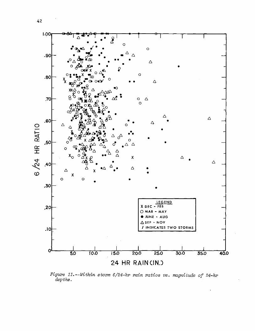
Figure 9 is a plot of the seasonal variation of the monthly 6/24 ratios for all the qualifying storms. The number of storms making up the averages, from a low of 10 in February to a high of 67 in September, are shown as well as the range in the ratio for each month. A fairly significant seasonal variation is indicated by the averages with generally higher ratios in the warm season. Figures lOa and lOb show maps of the 6/24 ratios for January and July, respectively. The data for January are too scanty to give a meaningful geographical pattern. We have identified certain ratios on the map for July (fig. lOb); those between 0.7 and 0.9 in boxes and those between 0.3 and 0.5 in circles to aid in discerning regional preference or bias in magnitude of the ratios. We conclude from the distributions shown that there is no significant regional pattern in magnitude of the ratios for our sample.
How the 6/24 ratios vary with rainfall magnitude is also of interest to our study. Figure 11 is a plot of the ratio vs. the 24-hr value in each ratio. Varying symbols are used to distinguish the four seasons. While a slight trend is shown in these data toward lower ratios with increasing 24-hr depths, one must be careful in interpreting this since all else being equal, the greater the 24-hr value (the denominator in the ratio) the lower the ratio. We conclude there is no signficant variation of 6/24 ratios with magnitude of the rainfall or season.
Plots were made for 72/24 ratios analogous to those for 6/24 ratios based on the same data base. Averages of these ratios by months (see fig. 12) show a smaller seasonal trend than for 6/24 ratios. Maps of the 72/24 ratios (not shown) give little evidence of regional patterns. As with the 6/24 ratios (see fig. 13) there is no significant trend in the 72/24 ratio with magnitude of the 72-hr rain.
4.7.2 Among Storms
Analyses of and compositing maps of the greatest observed rainfalls for 6-, 24-, and 72 hours implicitly sets 6/24 and 72/24 among storm ratios. these, along with the ratios given by HMR No. 51, were useful tools to our study.
4.7.3 Analyses
Since 6-, 24-, and 72-hr seasonal curves were plotted for the 20 grid points, the question of spacing between them comes up, that is, compatibility must be maintained in depth-duration relations. We strove for such compatibility through depth-duration plots for each grid point and month. Figure 14 is an example of these plots for 6 selected grid points for the month of November. On here are plotted transposed and moisture-maximized storm depths for all durations from 6 to 72 hours. Such plots insure that our 6-, 24-, and 72-hr PMP will properly envelop maximtm depths for other intermediate durations. Storms are identified by number (see table 2). At top of the plots for each grid point we also show rain ratios: 6- to 24-hr and 72- to 24-hr from the PMP and from the 4 percent probability level rainfall (part 4 of table 4). The ratios from rainfall frequencies are a guide to maintaining depth-durational consistency in the final product.

1.00 I I I ...,,.... I ...., I ....,,.... I -..- I -.- I ....,,.... I I I I
.9
0 .8
..... ~ .7
z <( .6 0:: 0:: .5 :r: ~ .4
~ <D .3
.2
.I
J ~ I;\ I I' II\ J - -....,, :>- I -
-r- - ..... ,, I' r -.- -l,.... J
:> f- ....,, -h .
4 ' o~ 4 4 -4
1- 4 4 -
o- 4 4 ' -4 - -
0- ,~ --''-
' ,If ,~ -'-
'~ -~ _._
o~ -'- -,~ v
-''-- --''- ,~ ,... ,It \l , -'--.'-- -'- --Or- ,,
-'- LEGEND -
'- .....,
o~ ±=RANGE -,... AVERAGE -o~
I -,
·,....
0 JAN FEB MAR .APR MAY JUN JUL AUG SEP OCT NOV DEC MONTH II 10 28 27 48 57 62 65 67 34 JS 19 #OFSTORMS
Figure 9. --Seasonal. variation of within storm 6/24-hr rain ratios for major storms in the study region. w
\C)

103°
-~
i i l_""'\_,
99°
~\. ... '"'
99"
95"
i --"1-,L_
- i
95"
I l \
Figure 10a.--Within stor,m 6/24-hr rain ratios 3 January.
91"
91" 87"
STA lUTE MILES -J2 190 ? I~ 200 3QO
1bo o 16o o 36o ~60 KILOMETERS
79° 75"
.s::-0

29''1--'----'--------'---'---""-,
XX RAIN RATIO • STORM LOCATION
2510 RATIOS .3-.6
D RATIOS .7 -.9 119' 115°
103' 99'
\ .. '-:
107' 103' 99'
Figure lOb.--Within storm 6/24-hr rain ratios~ July.
95' 91'
95' 91' 87'
STATUTE MILES
190 0 190 290 3QO
1 iJO 6 160 260 a6o 400
KILOMETERS
79' 75'
+:~
42
X 0 0 •
0
• •
X
•
0
0
0 6 0
•
• •
• •
•
•
LEGEND X DEC - FEB
QMAR-MAY
e JUNE - AUG
6SEP- NOV
•
6 •
I INDICATES TWO STORMS
24 HR RAIN CIN.)
FigUPe 11.--Within storm 6/24-hr rain ratios vs. magnitude of 24-hr depths.

2.00
1.90
1.80
0 1.70 -~ 0::
1.60
a:: :r: 1.50
~
~ 1.40 (\J 1'-
1.30
1.20
1.10
1.00
r-(2.28.1 I I I I I !_2,:!6) I I I I I (3_.~) I f-- •1\ II\ -. J -
'I' f- -.- -
LEGEND II\ 1-- -
tRANGE - .....
f- I -t-- AVERAGE -.-
II\ -....,,...
-,..-f- I I -t-- ...., .....
II\ -f- -1-- -f- l 1-- ___, ...,
1\ -J I
f- J 1--
1- 4
J 1--- 4 ~
1- ~ ~ -
~ 4
f--- -1- " \~ -
-''- -'-
1-_ -
' \~ \I
f- -'- ,~ _;._ -'-·~ ·~ \I -
\ '~ ...JL.... -1- -:-"- ....l:... -1- -
JAN FEB MAR APR MAY JUN JUL AUG SEP OCT NOV DEC MONTH 6 7 15 15~30 24 36 37 41 18 8 12 #OF
- STORMS
Figure 12.--Seasonal variation of within storm 72/24-hr rain ratios for major storms in the study region. .p.
w

44
0
t! 0::
z <( 0:::
0::: I
~
~ C\1 1'-
0
0
•
0
X 6
0
•
0 •
X
X •
X
6
0
X 0
X6
• xo
ooox •
6• 6xo
CD X X
• ~0
G>x oo 6• 0
~ 0 • (j
6
LEGEND X DEC- FEB
• OMAR- MAY
•
6
0 0
6 6•
• 6.
0 6
;. 6 • •
• JUNE- AUG 6SEP- NOV I INDICATES TWO STORMS
0
0
0
•
Figure 13.--Within storm 72/24-hr ra~n ratios vs. rmgnitude of 72-hr depths.
35.0

\J
-.J
~---------....... 1.5
0
3
68
1.5 1.5
0 1.0~
< c:: .5
•70 70
• 67 67
68
72 0 72
1.5 1.5 0
J.o i=
.5 5
69 69 • • • •
69 • • 66 •66 • 66
• ~9 69
72 72
DURATION CHR) DURATION CHR)
Figure 14.--Depth-duration plots for November (grid points 3~ 6~ 12~ 13~ 17~ 20). upper curves are the ratios of rainfall for various durations to the 24-hr values
<( c::
(+ from PMP; X from 4% probabili-ty values). Lower curves show PMP values. Maximized rainfall values transposed to the grid point are shown with storm number (table 2).
45

46
We found an inverse relation between the 6/24 ratio and that for 72/24. That is, if the 6/24 ratio is high, the 72/24 ratio is low, and visa versa. This appears to be meteorologically reasonable. For example, a high 6/24 ratio, expected in summer with brief thunderstorm type rainfall, is associated with a low 72/24 ratio.
4.8 Regional PMP Gradients
We have insistedPMP should not show sharp demarcations or changes from one point to the next unless explainable by terrain effects. Thus, we have plotted the 6-,:24-, and 72-hr PMP depths against selected latitudes and longitudes, covering the region in order to eliminate sharp changes. Figure 15 is an example of such plots •.•• showing 6-hr PMP along longitude 91°W for latitudes 30° to 47°N for each month.
4.9 Some Observations on PMP Patterns
The objectives or requirements of a) smooth patterns and gradients of PMP for each month and each duration (6, 24, 72 hours), b) smooth progression of increasing depths with duration, c) a smooth progression of PMP depths from month to month, and d) envelopment of moisture maximized and transposed storm rainfalls required numerous iterations. As one of the four objectives is approached, changes in analysis effect the other three. We should repeat a fifth objective uppermost in our thoughts during the study; this was to avoid undue indirect maximization and envelopment in achieving the objectives.
Some specific indications from the guidance material that were incorporated in the PMP patterns are as follows:
The semimonthly maximum w maps (see example in fig. 7a) indicate a gradual progression of moisturepfrom the Gulf Coast northward in early spring. A ridge of high moisture extending from the Gulf coast to the Great Plains can be identified easily in the summer months. The maximum w maps indicc::.te that moisture remains high through September. p
The maps of 4 percent probability rainfall also show higher values extending inland from the Louisiana and l1ississippi coasts during April and May than in adjacent months.
Maps of greatest observed rainfall depths show maximum precipitation in June in the northwestern portion of our study region. This set of maps reveals that maximum rainfall occurs in September along the eastern seaboard and in the gulf states. Scattered high values also appear in early October in some coastal regions, especially in Texas.
Some of the data, particularly the probability level values, showa longer season of maximum rainfall for the states bordering the Gulf and Atlantic coasts than for the interior regions. The plateau extends into September and early October. This can be explained by the greater opportunity for tropical

I"")
z \....1
a_ ~ a_
36r-----.-----.-----~----~------~----~-----r----~------r---~
--/ ____ ..... ""' /
/ /
/
/ /
/
/
/ /
NOV ,.,.,.,. ........ ....--------------_ ......
/
4~----~----L-----~----~~--~----~----~----~----~----~ 48 46 44 42 40 38 36 34 32 30 28
LATITUDE FigUX'e 15. --Latitudinal variation by month of 6-hr PMP aZong ZongitudinaZ 9JDW.
.p.
........

48
storm rainfall there •.•. and the fact that such storms can occur well into October. This aspect has been preserved in the seasonal variation of PMP. All-season PMP values extend to October for the coastal states and to September for much of the interior.
Comparison of maximum rainfall values in the interior for durations from 6 to 72 hours shows some tendency for peak values to extend over a longer season for 72 hours than for 6 hours. We find however, that the peak season for 24 and 72 hours have about the same length. This last indication has guided us to show the same length for all-season PMP for all durations.
5. RESULTING PMP
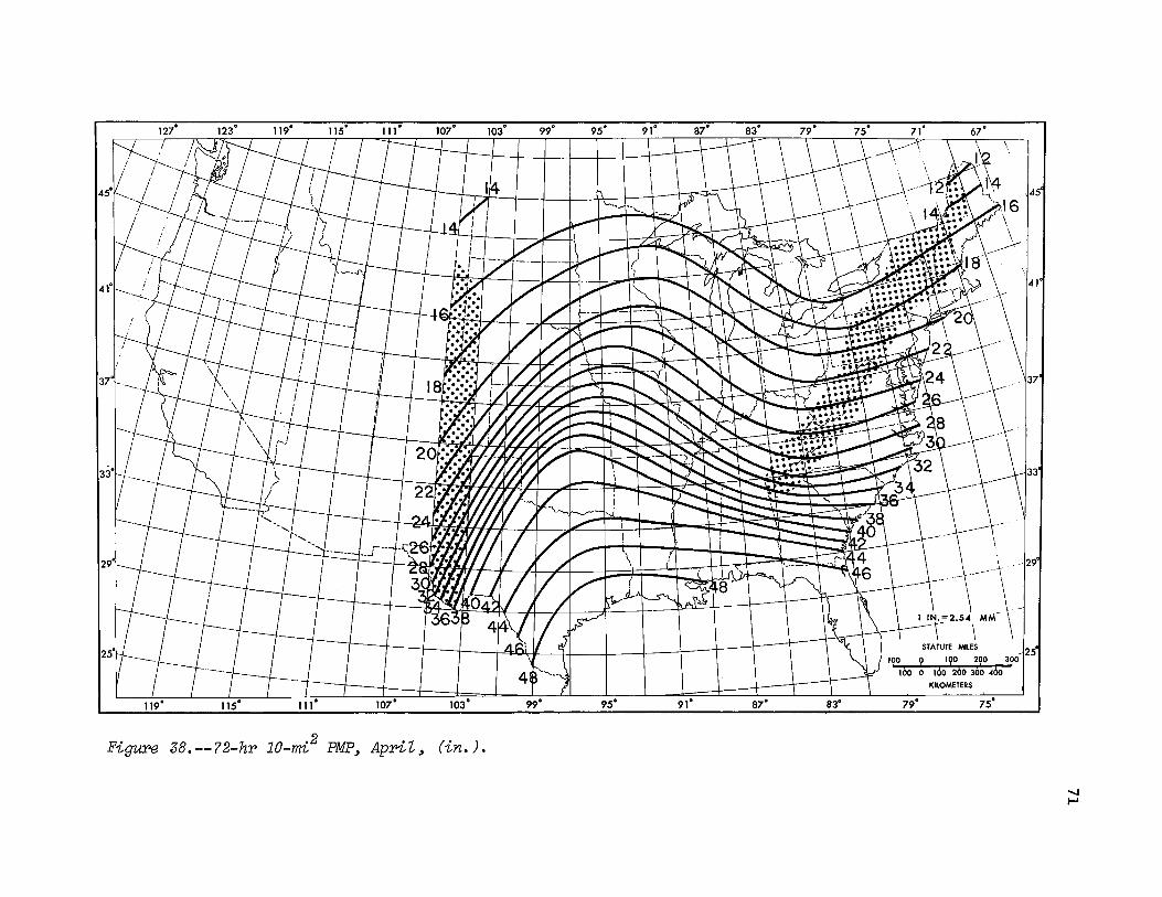
Figures 16 to 45 show midmonth maps of PMP for'6, 24, and 72 hours. A plot of depths for 6, 24, and 72 hours on a depth-duration chart joined by a curve through the point of origin (0,0) can be used to interpolate PMP for other durations. If PMP is required for some other data than midmonth, interpolate arithmetically.
6. EXAMPLE.OF USE OF PMP MAPS
In this example, assume 10-mi2 PMP is required for exactly April 8 for 22 hours duration at 40° 30'N latitude and 87°30'W longitude.
M.arch 15 April 15
a. 6-hr PMP (fig. 17) = 9.5 in. (fig. 18) = 13.1 in. 24-hr PMP (fig. 27) = 14.9 in. (fig. 28) = 19.0 in. 72-hr PMP (fig. 37) l8.8 in. (fig. 38) = 23.5 in.
b. Depth-duration plots (fig. 46) of these depths joined by smooth curves through (0,0) give 14.7 in. for March 15 and 18.9 in. for April 15, for 22 hours.
c. Linear interpolation for April 8 gives 18.0 inches.
7. SPECIAL PROBLEMS
7.1 Stippled Regions on PMP Maps
As for the all-season generalized PNP, our maps are stippled in two regions, (a) the Appalachian Mountains extending from Georgia to Maine and (b) a strip between the 103rd and 105th meridians. This stippling outlines areas within which the generalized PMP estimates might be deficient because detailed terrain effects have not been evaluated.
In developing the maps of PMP, it was sometimes necessary to transpose storms to or from higher terrain. Determination of storm transposition li~ts (par. 3.4.2) took into account topographic homogeneity in a general sense, thereby avoiding major topographic considerations. However, regional analysis required definition across mountains such as the Appalachians.

103° 99" 95" 91"
107" 103" 99" 95"
Figu:t'e 16.--6-hY' 10-mi2 PMP~ JanuaY'y and FebY'ua:ry ~ (in.).
91" 87" 83"
STATUTE MILES
190 ? 1\)0 2\)0 3QO 1 oo o ulo 260 JOo ~&;
KILOMETERS
79" 75°
.j:-\0

103' 99' 95'
107' 103' 95'
Figur'e 17.--6-hr 10-mi2 PMP, MaY'ch, (in,).
91'
91' 87' 79'
KILOMETERS
75'
V1 0

103° 99° 95° 91°
107° 103° 99° 95"
Figu:I'e 18.--10-mi2
PMP3 April 3 (in.).
91° 87.
STATUTE MILES
190 ? IQO 290 3QO 1 oo o ulo 260 aoo 40o
KILOMETERS
79" 75°
l..n 1-'

99° 95" 91°
107" 103° 99" 95°
Figure 19.--6-hr 10-mi2 PMP~ May~ (in.).
91° 87° 83° 79°
KILOMETERS
75°
U1 N

103° 99° 95' 91'
107' 103' 99' 95'
Figure 20.--6-hr 10-mi2 PMP, June~ (in,).
87'
91' 87'
STATUTE MILES
.190 0 IQO 290 3QO
1 bo 6 ulo 26o J6o ~& KILOMETERS
79' 75°
Vl w

99° 95° 91°
107° 103° 95" 91°
Figure 2"1. -;-6-hr 10-mi2 P~ July and August_, (in.).
87" 83"
STATUTE MILES
190 0 IQO 2QO 3QO
1 iJO 6 ulo 260 30o ~bo KILOMETERS
79" 75"
1.../1 .j::-

127° 103° 99° 95" 91"
107° 103° 95"
Figure 22.--6-hr 10-mi2 PMP~ September~ (in.).
91° 87'
STATUTE MILES
190 0 190 290 JQO
1 oo o ulo 26o J6o ~&o KILOMETERS
79" 75°
ln ln

127° 107° 103' 99° 95'
107" 103" 95"
Figure 23. --6-hr lO-mi2 PMP3 October 3 (in.).
91'
91° 87"
STATUTE MILES
1?0 0 IQO 2QO 3QO
u\o 6 ulo 200 Joo 4d0 KILOMETERS
79' 75°
U1 0'\

99" 95" 91"
107" 103° 95" 91°
Figure 24.--6-hP 10-mi2 PMP, NovembeP, (in.).
87"
STATUTE MILES
100 0 190 2?0 390
100 6 TOO 260 300 400 KILOMETERS
79" 75°
ln -.....!

103° 99° 95" 91°
107" 103° 99" 95"
Figure 25.--6-hr 10-mi2 PMP, December, (in.).
91° 87" 83°
STATUTE MILES
100 ? 190 2?0 3?0 1 oo o ulo 260 3oo ~Cio
KILOMETERS
79° 75°
V1 CXl

127° 123° 115" 111° 107° 103° 99° 95° 91°
107° 103° 99" 95° 91° 87"
Figure 26.--24-hr 1D-mi2 PMP3 January and February 3 (in.).
,.--:"
\
-~\-- \ I \. IN.>=2.54 MM--
- \ \ STAJUTE MUS
100 y 1?0 2qo 3qo Jilo 0 lbo 2CSO 3Clo :;&;
KI.OMOB!S
79" 75"
45'
41
37
129'
V1 1.0

103° 99" 95° 91°
107° 103° 95"
Figure 27.--24-hr 10-mi2 PMP, March, (in.).
91° 87°
STATUTE MILES
IQO ? TQO 2QO JQO
100 0 .6o 260 J6o .60 KILOMETERS
79" 75°
0'\ 0

103° 99° 95° 91°
107° 103" 99° 95°
Figure 28.--24-hP 10-mi2 PMP, April, (in.).
91° 87"
STATUTE MILES
190 0 lQO 290 3QO
1bo b 100 26o JOo 460 KILOMETERS
79° 75°
0\ ,......

103° 99° 95° 91°
107° 103° 99. 95.
Figure 29. --24-hr 10-mi2 PMP_, May_, (in.).
91. 87° 83°
STATUTE MILES
IQO 0 IQO 290 3QO
1bo 6 160 26o J6o 400 KILOMETERS
79" 75°
"' N

103° 99' 95' 91'
107' 103' 99' 95' 91'
Figure 30.--24-hr 10-mi2
PMP, June, (in.).
87' 83'
I
STATUTE MILES
190 ? 190 290 3QO 100 o 16o 260 a6o 400
KILOMETERS
79' 75'
'25'
0'\ w

103° 99' 95'
107' 103' 99' 95' 91' 87'
Figure Jl.--24-hr 10-mi2 PMP, July and August, (in.).
45
41
-r~·, \
STATUTE MILES
190 0 1?0 290 390
1 oo 6 ulo 26o 30o 46o KILOMETERS
79' 75'
0"1 .j::-.

103° 99° 95" 91°
107" 103° 95"
Figure 32.--24-hr 10-mi2 PMP3 September 3 (in.).
91" 87"
STATUTE MILES
190 ? 190 290 390 100 o 1bo 260 Jbo 40o
KILOMETERS
79" 75"
0\ U1

103° 99° 95" 91°
107" 103" 99" 95"
.2 . (. ) Figure 33,. --24-hr 10-m'/... PMP~ October~ 1..-n • •
91" 87" 83"
STATUTE MILES . -125. 190 ? lQO 290 3QO
1 oo o ulo 26o Joo 400
KILOMETERS
79" 75°
(j\ (j\

99° 95° 91°
107° 103° 95° 91°
Figure 34.--24-hr 10-mi2 PMP~ November~ (in.).
87° 83°
STATUTE MILES -J25
190 ? 1?0 2?0 3?0
1 oo o ulo 26o 300 46o KILOMETERS
79° 75°
0\ --..1

103' 99' 95' 91°
107' 103' 99' 95°
Figure 35.--24-hr 10-mi2 PMP~ December~ (in.).
91° 87'
STATUTE MILES
100 0 1QO 2QO 3QO
100 6 100 26o JOo ~&o KILOMETERS
79° 75'
0'1 CX>

99" 95• 91"
107° 103. 99. 95•
Figure 36.--?2-hr 10-mi2 PMP, January and February, (in.).
91. 87.
STATUTE MILES
100 0 lQO 2\)0 3QO
1 oo 6 ulo 260 300 400 KILOMETERS
79. 75°
0'\ 1.0

99° 95" 91"
37
107" 103° 95° 91" 87"
Figure 3?. -- ?2-hr 10-mi2
PMP, March_, (in.).
··'45'
41
_ _,_ ... -·!29' I
lQO ? IQO 2QO 3QO ' 1 bo o ulo 260 Jbo 400
KILOMETERS
79" 75"
25'
....... 0
103° 99° 95° 91°
107° 103° 99° 95° 91° 87°
Figure 38.--72-hr 10-mi2 PMP~ ApriZ~ (in.).
-rl\.-IN.=2.54 MM-
~ \ \ STATUTE MILES
100 ? IQO 2QO 3QO
1 oo o ulo 260 aoo 460 KILOMETERS
79° 75°
45
41
-·29'
25'
'-I ,_.

103' 99° 95' 91'
107' 103' 95' 91'
Figure 39.--?2-hr 10-mi2 PMP~ May~ (in.).
87' 83'
STATUTE MILES
190 ? 190 290 390 1 bo o u\o 260 Jbo ~6o
KILOMETERS
79' 75°
25
-....J N

103° 99° 95• 91°
107° 103° 95° 91° 87.
Figure 40.--72-hr 10-rrri2 PMP, June, (in.).
,.
--\ .-...l,-
I
I~.':J.J MM. \
-~
..41
29'
100 ? 1?0 200 3?0 ·25
' 1 oo o ulo 260 3oo 46o
STATUTE MILES
KILOMETERS
79. 75°
...... w

103° 99° 95° 91°
107° 103° 99" 95"
Fi(JUT'e 41. --?2-hr 10-mi2 PMP~ JuZy and August~ (in.).
91" 87"
STATUTE MILES
100 0 1\)0 2QO 3QO
10o 6 160 260 300 ~30 KILOMETERS
79° 75°
....... ~

103° 99° 95°
107° 103" 95° 91° 87°
Figure 42.--?2-hr 10-mi2 PMP3 September3 (in.).
STATUTE MILES
190 9 190 290 390 1bo o 100 26o 3oo 400
KILOMETERS
79° 75°
45
41
·29'
25'
" V1

103° 99° 95" 91°
107° 103° 95° 91"
Figure 43.--?2-hr 10-mi2 PMP~ October~ (in.).
87' 83"
STATUTE MILES
100 0 IQO 2QO 3QO
1 bo 6 ulo 260 Joo 400
KILOMETERS
79' 75'
....... 0\

103° - 99° 95" 91"
107° 103° 99" 95"
Figu:r'e 44·. -- ?2-hr 10-mi2 PMP, Noverriher, (in.).
91" 87"
STATUTE MILES
100 ? IQO 2QO 3QO
1 oo o ulo 260 Joo 460 KILOMETERS
79" 75°
...... ......

103° 99° 95° 91°
107" 103" 99° 95"
Figure 45.--72-hr 10-mi2 PMP3 December~ (in.).
91" 87" 83"
STATUTE MILES
100 ? 1\)0 2QO JQO
1 oo o ulo 260 JOO ~110 KILOMETERS
79" 75°
-...! 00

30.---.---.-~r-~--~--~--~--~--~--~--~--~----
25 APRIL IS
~ . z v 201 ------- MARCH IS
F= 0.
~ 15
0. ~ 0..
0 so 66 72
Figure 46.--ExampZe of variation of PMP depths with duration for mid-month of March and ApriZ for 40.5°N 8?.5°W (see sec. 6). --.!
1.0

80
For such regions, the assumption was made that the reduced height of the column of moisture available for processing at higher elevations is compensated by intensification from steeper terrain slopes at these higher elevations.
In contrast to the use of these simplifying assumptions, studies of PMP covering portions of the Western States (U.S. Weather Bureau 1961, 1966, and Hansen et al. 1977) and Tennessee River drainage (Schwarz and Helfert 1969) do take into account detailed terrain effects. A laminar flow orographic precipitation computation model, useful in some regions where cool-season precipitation is of greatest concern, gave detailed definition for some of the Western States. For the Tennessee River drainage, nonorographic PMP was adjusted for terrain effects by considering numerous different rainfall criteria and taking into account meteorological aspects of critical storms of record.
We expect future studies of the Hydrometeorological Branch will involve detailed generalized studies covering the stippled regions. Until these studies are completed, we suggest that major projects within the stippled regions be considered on a case-by-case basis as the need arises.
7.2 Extreme Precipitation at Mt. Washington, N.H.
Some very extreme precipitation values have been observed in winter at Mt. Washington, a location in the stippled regions of the PMP maps. Three of the most extreme are listed in table 5. The editor of the Mount Washington Observator-y News Bulletin gives the following description of the February 10-11, 1970 storm:
On the lOth and 11th there was a little storm that deposited a whopping 10.12 inches of water equivalent into the precipitation gage in 24 hours for another new record in this department! DuPing part of the storm dense ice accumulated at the rate of five inches per hour and Summit structure eventually exhibited accumulations two feet thick in places. Wind during the storm peaked at 128 mph.
Since Mount Washington Observatory, at an elevation of 6,262 feet, is located well above the mean elevation in the region we did not attempt to transpose such precipitation to other locations. We did not make adjustments for maximum moisture, but did ensure that the observed values were enveloped by the PMP isolines.
7.3 Point Rainfall vs. 10 mi 2 Average Rainfall
This study estimates PMP for 10-mi2 areas. The basic data (Corps of Engineers, U.S. Army 1945- ) often use point rainfall as 10-mi2 rainfall depths. This is done in order to at least par.tially compensate for the slim chance of catching the most intense rainfall in any storm. The question may then be raised as to whether PMP for areas less than 10 mi2 would be greater than the 10-mi2 values of this report. For the all-season PMP taken.from HMR No. 51, this is answered by the fact that with few exceptions the

81
TabZe 5.--Extreme precipitation amounts observed at Mt. Washington~ N.H. (44°16N; ?l 0 18W) during the winter season.
Durat.i.on (hr) 6 12 18 24 48 72
Storm date Recorded precipitation amounts (in.)
Feb. 10-11, 1970 4.7 9.2 10.1
Dec. 26-28, 1969 3.3 8.6 10.2 10.3
Feb. 25-27, 1969 3.4 8.4 12.5 14.1
critical storm values establishing PMP for 10 mi2 came from 10-mi2 average rainfalls rather than single station values. Therefore, all-season PMP for areas less than 10 mi2 exceed those given here for 10 mi2 .
What about storms controlling other seasons? PMP estimates for points during the cool season, ~ay October - April, would reasonably be not much different from the 10-mi values given in this report. This is so, since in winter rains are less variable from place to place because there is much less convective activity than in summer.
7.4 Storm Adjustments Greater than 150 Percent
Extreme increase in one parameter, say moisture, could well counteract other important factors; therefore, total storm adjustments that increased rainfalls by more than 50 percent were given further attention. If a storm had an adjustment giving an increase greater than 50 percent, but its adjusted depth was supported quite closely by surrounding storm depths with only moderate adjustments, the high adjusted value was accepted. If a high adjustment (greater than 50 percent) gave an amount that stood out among all other storms in a region, a value obtained by multiplying the observed depth by 150 percent was used. This limitation was also applied to HMR No. 51.
8. OBSERVED STORMS WITHIN 50 PERCENT of PMP
To give the user some insight on the magnitude of PMP, we have identified the known storm depths that are~ 50 percent of PMP. For simplification the PMP for the midmonth in which the storm occurred is compared with the storm depth. For example, if a storm occurred on any day in March it is compared with PMP for mid-March. A March 1 storm would actually be a higher percent of March 1 PMP and a March 31 storm would be a lower percent of March 31 PMP. No comparisons were made for July and August, the months for which we accept the all-season PMP of HMR No. 51. Comparisons of observed rainfall to allseason PMP in HMR No. 51 are given by Riedel and Schreiner, 1980.
Figure 47 shows a seasonal plot of the number of known storms that are > 50 percent of lO-mi2 PMP for 6, 24, and 72 hours. As discussed earlier, undoubtedly, many more storms have reached 50 percent of PMP than have been sampled by the sparse network. That there are fewer cases in winter than

(/)
~ 0::: 0 I(/)
LJ.... 0
0::: w co ~ ::J z
20----------~----~--~~--~--~~----~
• •
• • • • •
• • •
Figure 4?.--Number of separate storms with rainfall ~50% of PMP for 6~ 24~ and ?2 hours (number of storms > 50% of PMP for July and August can be obrained from Riedel and-Schreiner 1980).
00 N

summer is in the right direction: fewer storms have been studied in the cool season and fewer surveys made after storm events to find extremes.
Table 6 lists chronologically the storms that have observed depths ~ 50 percent of PMP for each month. Some of course are identical to the major storms of table 2.
83
We only show comparisons for rainfall depths for 6, 24, and 72 hours. If more durations were added (between 6 and 72 hours) many more storms would reach 50 percent of PMP and the percentages shown would be higher.

84
Table 6.--Known stoPm rainfalls for 6, 24 and 72 hours that are within 50 peraent of mid-month PMP for the month in whiah the stoPm oaaurred (July and August stoPms not inaluded)
Obs. COE Storm Dur. Precip. % of Assign.
Date number Lat. Long. (hrs) (in.) PMP No. Source*
Jan.l-2,1941 3 48°00 89°42 24 4.7 65 TP No. 16 Jan.22-27,1949 5 35°52 92°19 6 7.5 52 SW3-10 STR
24 11.7 54 Feb. 2-18,1883 41°42 77°16 6 3.6 60 ORS-11 STR Feb.l2,1886 41°54 71°23 24 7.9 56 STR Feb.6,1960 43°07 73°35 24 5.1 61 DTD
Feb.25-27,1969 12 44°16 71°18 24 8.4 86 DTD 72 14.1 68
Feb.l0-11,1970 13 44°16 71°18 6 4.7 89 DTH 24 10.2 100
Feb.l,1973 14 32°56 92°36 6 10.6 65 DTH Mar.13,1888 42°43 73°18 24 6.1 52 TP No. 16 Mar.28,1902 35°41 85°48 24 11.0 so TP No. 16
Mar.23-27,1913 17 40°22 83°46 24 7.3 55 ORl-15 STR 72 10.4 61
Mar.11-16,1929 19 31°25 86°04 6 14.0 73 LMV2-20 STR 24 20.0 65 72 29.6 74
Mar.12,1936 44°16 71°15 24 6.5 66 TP No. 16 Mar.22,1949 44°25 72°16 24 s.o 55 TP No. 16
(update) Mar.31,1951 41°56 74°23 24 6.7 57 TP No. 16
(update)
Mar.25,1964 21 35°37 84°12 6 7.5 55 DTH Mar.16-18,1965 22 46°53 90°49 72 6.6 54 DTD l·lar.25,1965 41°34 75°52 6 4.3 57 DTH Mar.2-5,1966 23 47°14 98°35 24 4.7 57 STR Mar.14,1973 24 44°21 103°46 24 5.7 71 DTD
Apr.11-14,1933 26 43°08 70°56 6 4.9 52 NAl-23 STR Apr.3-4,1934 27 35°37 99°40 6 17.3 73 SW2-11 STR Apr.24-28,1937 28 39°40 77°54 72 11.3 53 SAS-13 STR Apr.21,1951 33°21 94°30 6 14.2 53 DTH May 30-June 1,
1889 41°45 77°17 6 7.4 53 SAl-1 STR
May 30-31,1935 34 39°36 102°08 6 16.5 82 MR 3-28A STR 24 22.2 83
May 6-12,1943 35 35°29 95°18 72 24.9 56 SW2-20 STR May 12-20,1943 35°52 96°04 6 15.9 56 SW2-21 STR June 13-18,1886 38 31°19 92°33 72 29.0 53 LMV4-27 STR June 2.7-Jul.l,
1899 30°52 96°32 72 34.5 64 STR
June 17-21,1921 39 47°18 105°35 6 10.5 55 MR4-21 STR 24 13.3 53 72 14.6 53
June 30,1932 30°01 99°07 24 31.7 75 GMS-1 STR June 19-20,1939 32°44 100°55 6 13.8 71 STR June 10-13,1944 41°52 97°03 6 13.4 53 MR6-15 STR June 23-24,1948 42 29°22 100°37 24 26.2 66 STR June 23-28,1954 43 30°12 101°35 6 16.0 61 SW3-22 STR
24 26.7 71 72 34.6 77
See notes at the end of the table.

85
TabZe 6.--Known storm rainfaZZs for 6, 24 and 72 hours that are within 50 peraent of mid-month PMP for the month in whiah the storm oaaurred (JuZy and August sto1'11ls not ina Zuckd) (Continued)
Obs. COE Storm
£#fs) Precip. % of Assign.
Date number Lat. Long. (in) PMP No. Source
June 8-10,1962 44°12 103°31 72 14.9 62 DTD June 23-24,1963 45 41°14 97°05 6 14.6 57 STR
24 16.2 51 June 24,1966 46 47°21 101°19 6 11.1 53 STR June 9,1972 47 44°12 103°13 24 14.9 54 MRl0-12 STR June 20-22,1972 48 42°05 78°10 24 14.3 52 NA2-24A STR
72 18.5 58
Sept.8-10,1921 49 30°35 97°18 6 22.4 74 GM4-12 STR 24 36.5 84 72 37.6 72
Sept.17-19,1926 so 43°12 96°00 6 15.1 62 MR4-24 STR 24 21.7 71
Sept.14-18,1936 31°47 100°50 24 26.0 68 STR 72 30.0 65
Sept.1,1940 52 39°42 75°12 6 20.1 76 NA2-4 STR Sept.2-6,1940 53 36°15 96,0 36 6 18.4 65 SW2-18 STR
24 23.6 64
Sept.J-7,1950 54 29°03 82°42 24 38.7 81 SAS-8 STR 72 45.2 82
Oct.7-11,1903 56 40°55 74°10 24 13.7 51 GL4-9 STR Oct.l7-22,1941 57 29°48 82°57 24 30.0 73 SAS-6 STR
72 Js;o 66 Oct.ll-18,1942 58 38°31 78°26 72 18.7 52 SA1-28A STR Oct.30-Nov.l, 70 30°41 81°28 24 22.0 67 DTD
1969 72 22.6 56
Oct.lQ-11,1973 63 36°25 97°52 6 16.9 77 STR Nov.7,1915 65 48°54 103°18 24 4.0 56 TP No. 16 Nov.2-4,1927 67 44°03 71°45 6 7.8 78 NAl-17 STR
24 12.0 79 72 14.0 71
Nov.22-25,1940 69 30°08 96°08 24 18.6 59 GMS-13 STR 72 21.1 53
Nov.1,1948 37°02 99°59 6 6.1 so DTH
Nov.13,1954 24°33 81°48 24 19.9 62 TP No. 2 Dec.S-8,1935 72 29°54 95°37 24 18.6 66 GMS-4 STR
72 20.8 57 Dec.29-Jan.l,
1949 73 42°40 73°19 24 8.1 62 NA2-18 STR 72 12.6 73
Dec.20,1959 37°25 82°01 6 6.7 56 DTrl Dec.26-28,1969 74 44°16 71°18 6 3.3 55 DTD
24 8.6 77 72 10.4 70
Dec. 26-28,1969 44°40 70°09 24 6.0 51 TP No. 16 72 10.0 71 (update)
COE: Corps of Engineers
* Source STR.: Storm rainfall TP No. 16: Technical Paper No. 16 DTD: Data tape; daily precipi~ation DTH: Data tape;.hourly precipitation

86
ACKNOWLEDGEMENTS
The authors thank J. Miller, Chief, Water Management Information Division and Dr. Vance A. Myers, Chief, Special Studies Branch for reviewing the study. They also wish to thank meteorologists L. Schreiner, R. Watkins and R. Zehr, technicians Marion Choate, Teresa Johnson, Roxanne Johnson, Normalee Foat and Keith Bell for assistance and Virginia Hostler, Clara L. Brown, and Donna Smith for typing the numerous versions of this report.

REFERENCES
American Meteorological Society, 1959: Glossary of Meteorology. Boston, Mass., 638 pp.
87
Atmospheric Environment Service, 1961-: Storm Rainfall in Canada, Downsview, Ontario, Canada.
Atmospheric Environment Service, Canada 1973: Canadian Normals, Volume 2 Precipitation 1941-1970, Downsview, Ontario, Canada, 330 pp.
Department of Transport, Het:orological Branch 1970: Climatological Station Data Catalogue: The Prairie Provinces, CL14-70, 126 pp; Ontario CLlS-70, 90 pp; Quebec CL16-70, 65 pp; fhe Atlantic Provinces, CL17-70, 46 pp.
Department of Transport, Meteorological Branch --, Maximum Precipitation Reported on Any One Observation day, 1931-1958 (unpublished report).
Environmental Data Service, 1968: Maximum persisting 12-hour 1000-mb dew points (°F) monthly and of record. Climatic Atlas of the United States, Environmental Science Services Administration, U.S. Department of Commerce, Washington, D.C., pp. 59-60.
Frederick, Ralph H., Myers, Vance A., and Auciello, Eugene P., 1977: Fiveto 60-Minute Precipitation Frequency for the Eastern and Central United States. NOAA Technical Memorandum NWS HYDR0-35, u.s. Department of Commerce, Silver Spring, Md., 36 pp.
Hansen, E.M., Schwarz, Francis K., and Riedel, John T., 1977: Probable Maximum Precipitation Estimates, Colorado River and Great Basin Drainages, Hydrometeorological Report No. 49, National Weather Service, National Oceanic and Atmospheric Administration, U.S. Department of Commerce, Silver Spring, Md., 161 pp.
Hershfield, David M., 1961: Rainfall Frequency Atlas of the United States for Durations From 30 Minutes to 24 Hours and Return Periods from 1 to 100 Years. Technical Paper No. 40, Weather Bureau, U.S. Department of Commerce, Washington, D.C., 115 pp.
Ho, F. P., and Riedel, John T., 1979: Precipitable Water over the United States Volume 2: Semimonthly Maxima. NOAA Technical Report NWS No. 20, U.S. Department of Commerce, Silver Spring, Md., 359 pp.
Jennings, Arthur H., 1952: Maximum 24-Hour Precipitation in the United States. Technical Paper No. 16, Weather Bureau, U.S. Department of Commerce, Washington, D.C., 284 pp.
Jennings, A.H., (revised) 1963: Maximum Recorded United States Point Rainfall for 5 Minutes to 24 Hours at 296 First-Order Stations. Technical Paper No. 2, Weather Bureau, U.S. Department of Commerce, Washington, D.C., 56 pp.

88
Miller, John F., 1963: Probable Maximum Precipitation and Rainfall-Frequency Data for Aiaska. Technical Paper No. 47, Weather Bureau, U.S. Department of Commerce, Washington, D.C., 69 pp.
Riedel, John T., Appleby, James F., and Schloemer, Robert W., 1956: Seasonal Variation of the Probable Maximum Precipitation East of the 105th Meridian for Areas From 10 to 1000 Square Miles and Durations of 6, 12, 24 and 48 Hours. Hydrometeorological Report No. 33, Weather Bureau, u.s. Department of Commerce, Washington, D.C., 58 pp.
Riedel, John T., and Schreiner, L.C., 1980: Comparison of Generalized Estimates of Probable Haximum Precipitation \-lith Greatest Observed Rainfalls NOAA Technical Paper, (in preparation).
Schreiner, L.C., and Riedel, John T., 1978: Probable Maximum Precipitation Estimates, United States East of the 105th Meridian. Hydrometeorological Report No. 51, National Weather Service, National Oceanic and Atmospheric Administration, Silver Spring, Md., 87 pp.
Schwarz, Francis K., 1965: Probable Maximum and TVA Precipitation Over the Tennessee River Basin Above Chattanooga. Hydrometeorological Report No .. 41, Weather Bureau, U.S. Department of Commerce, Washington, D.C., 148 pp.
Schwarz, Francis K., and Helfert, Norbert F., 1969: Probable Maximum and TVA precipitation for Tennessee River Basins Up to 3000 Square Miles in Area and Durations to 72 Hours. Hydrometeorological Report No. 45, Weather Bureau, Environmental Science Services Administration, U.S. Department of Commerce, Silver Spring, Md., 166 pp.
Shipe, Albert P., and Riedel, John T., 1976: Greatest Known Areal Storm Rainfall Depths for the Contiguous United States. NOAA Technical Memorandum NWS HYDRO 33, National Weather Service, National Oceanic and Atmospheric Administration, U.S. Department of Commerce, Silver Spring, Md., 174 pp.
U.S. Army, Corps of Engineers, 1945-: Storm RainfaU in the United States, Depth-Area-Duration Data, Washington, D.C. (ongoing publication).
U.S. Weather Bureau, 1947: Generalized Estimates of Maximum Possible Precipitation Over the United States East of the 105th Meridian, for Areas of 10, 200,, and 500 Square Miles. Hydrometeorological Report No. 23, U.S. Department of Commerce, Washington, D.C., 77 pp.
U.S. Weather Bureau, 1951: Tables of Precipitable Water and Other Factors For a Saturated P.seudo-Adiabatic Atmosphere. Technical Paper No. 14, U.S. Department of Commerce, Washington, D.C., 27 pp.
U.S. Weather Bureau, 1951-61: Maximum Station Precipitation for 1, 2, 3, 6, 12, and 24 hours, Part I: Utah, Part II: Idaho, Part III: Florida, Part IV: Maryland, Delaware and District of Columbia, Part V: New Jersey, Part VI: New England, Part VII: South Carolina, Part VIII: Virginia, Part IX: Georgia, Part X: New York, Part XI: North Carolina~

Part XII: Oregon, Part XIII: Kentucky, Part XIV: Louisiana, Part XV: Alabama, Part XVI: Pennsylvania, Part XVII: Mississippi, Part XVIII: West Virginia, Part XIX: Tennessee, Part XX: Indiana, Part XXI: Illinois, Part XXII: Ohio, Part XXIII: California, Part XXIV: Texas, Part XXV: Arkansas, Part XXVI: Oklahoma. TechnicaZ PapeP No. 15, Department of Commerce, Washington, D.C.
89
U.S. Weather Bureau, 1961: Interim Report Probable Maximum Precipitation in California. HydrometeoPo"logicaZ RepoPt No. 36, U.S. Department of Commerce, Washington, D.C., 202 pp.
U.S. Weather Bureau, 1966: Probable Maximum Precipitation, Northwest States. HydPometeoPo"logicaZ RepoPt No. 43, Environmental Science Services Administration, U.S. Department of Commerce, Washington, D.C., 228 pp.
World Meteorological Organization, 1973: Manual for Estimation of Probable Maximum Precipitation, WMO No. 332, OpePationaZ HydroZogy RepoPt No. 1, Geneva, Switzerland, 190 pp.
<r U. S. GOVERNMENT PRINTING OFFICE_: 1980 311-046/126

NOAA--S/T 80-65' ' '